Quasi-incompressible Multi-species Ionic Fluid Models

Abstract

In traditional hydrodynamic theories for ionic fluids, conservation of the mass and linear momentum is not properly taken care of. In this paper, we develop hydrodynamic theories for a viscous, ionic fluid of $N$ ionic species enforcing mass and momentum conservation as well as considering the size effect of the ionic particles. The theories developed are quasi-incompressible in that the mass-average velocity is no longer divergence-free whenever there exists variability in densities of the fluid components, and the models are dissipative. We present several ways to derive the transport equations for the ions, which lead to different rates of energy dissipation. The theories can be formulated in either number densities, volume fractions or mass densities of the ionic fluid components. We show that the theory with the Cahn-Hilliard transport equation for ionic species reduces to the classical Poisson-Nernst-Planck (PNP) model with the size effect for ionic fluids when the densities of the fluid components are equal and the entropy of the solvent is neglected. It further reduces to the PNP model when the size effect is neglected. A linear stability analysis of the model together with two of its limits, which is the extended PNP model (EPNP defined in the text) and the classical PNP model (CPNP) with the finite size effect, on a constant state and a comparison among the three models in 1D space are presented to highlight the similarity and the departure of this model from the EPNP and the CPNP model.

Keywords: Ionic fluids, phase field, quasi-incompressibility, hydrodynamics.

1 Introduction

Phase field models have been used successfully to study a variety of multiphasic phenomena like equilibrium shapes of vesicle membranes [13, 14], blends of polymeric liquids [52, 53, 54, 17], multiphase fluid flows [19, 25, 34, 38, 35, 58, 57, 59, 61, 63], dentritic growth in solidification, microstructure evolution [21, 40, 28], grain growth [9], crack propagation [10], morphological pattern formation in thin films and on surfaces [36, 45], self-assembly dynamics of two-phase monolayers on an elastic substrate [37], a wide variety of diffusive and diffusion-less solid-state phase transitions [11, 56], dislocation modeling in microstructure, electro-migration and multiscale modeling [49]. Multiple phase-field methods can be devised to study multiphase materials [57]. Recently, phase field models are applied to study liquid crystal drop deformation in another fluid, liquid films, polymer nanocomposites, biofilms and cells [19, 25, 34, 38, 35, 58, 57, 59, 61, 62, 18, 64, 32, 65, 66, 67].

Comparing to other mathematical and computational technologies available for studying multi-phase materials, the phase-field approach exhibits a clear advantage in its simplicity in model formulation, ease of numerical implementation, and the ability to explore essential interfacial physics at the interfacial regions etc. Computing the interface without explicitly tracking the interface is the most attractive numerical feature of this modeling and computational technology. Since the pioneering work of Cahn and Hilliard in the 50’s of the last century, the Cahn-Hilliard equation has been the foundation for various phase field models [7, 8]. It arises naturally as a model for multiphase material mixtures should the entropic and mixing energy of the mixture system be known.

While modeling immiscible binary fluid mixtures using phase field theories, one commonly uses a labeling or a phase variable (also known as a volume fraction or an order parameter) $\phi$ to distinguish between distinct fluid phases. For instance $\phi=1$ indicates one fluid phase while $\phi=0$ denotes the other fluid phase in an immiscible binary mixture. The interfacial region is tracked by $0<\phi<1$. For historical more than logical reasons, most mixing energies are calculated in terms of the volume fraction instead of the mass fraction in the literature [20, 12]. Consequently, the system free energy including the entropic and mixing contribution has been formulated in terms of the volume fraction as well [20, 12], given in the form $F[\phi,\nabla\phi,\cdots]$. A transport equation for the volume fraction $\phi$ along with the conservation equation of momentum and the continuity equation constitute the essential part of the governing system of hydrodynamic equations for the binary fluid mixture, where the volume fraction serves as an internal variable for the fluid mixture.

In this formulation, the material incompressibility is often identified with the continuity equation

$$\begin{array}[]{l}\nabla\cdot{\bf v}=0.\end{array}$$ (1.2)

This assumption is plausible and indeed consistent with the fluid incompressibility (1.2) only if the two fluid components in the mixture are either completely separated by phase boundaries when their densities are not equal or possibly mixed when the densities are identical. Otherwise, there is a potential inconsistency with the conservation of mass as well as conservation of linear momentum. This inconsistency has been identified in [38], but ignored by many practitioners using phase field modeling technologies for hydrodynamical systems. We note that this inconsistency occurs only in the mixing region of the two incompressible fluids, where the incompressibility condition (1.2) is no longer valid, indicating the mixture is no longer incompressible despite that each fluid component participating in mixing is. This type of fluids is referred to as quasi-incompressible in [38]. A systematic fix to this problem for mixtures of incompressible viscous fluids was given by two of the authors in [31], where the divergence free condition is modified to accommodate the quasi-incompressibility.

In modeling of ionic fluids, one recognizes that the size of ions matters in most ionic solutions, in particular in the ionic solutions in which life occurs, in the ocean, and of course in the very crowded conditions found in and near electrodes in batteries and electrochemical cells, in and around enzymes, ionic channels, transporters, and nucleic acids, both DNA and RNA [68]. Ionic solutions are hardly ever ideal: ionic size is almost always important. In multispecies ionic fluids above a certain concentration or under certain length scales, the size of the ions matters so that the same inconsistency issue in the models for ionic solutions arises again. That is one can not simply use the solenoidal condition in the velocity field as a proxy for the material incompressibility. A theory for multispecies ions of incompressible fluid flows that respects the material’s mass conservation and momentum conservation needs to be developed.

This paper aims exactly at developing such a theory for a mixture of ionic fluid flows of multiple ionic species, in which the ionic densities are unmatched and different from that of the solvent, and their size effects are non-negligible. We require the theory to be dissipative while conserving mass and momentum. One targeted application of this theory is in ion channel modeling [15, 16, 26]. Ion channels provide enough data to distinguish between theories because measurements are available over a wide range of conditions [5, 6]. Hundreds of channel types are studied every day because of their biological and clinical significance [68]. Concentrations and electrical potentials are controlled in experiments and these provide sets of values for boundary conditions of mathematical models. Fitting the entire set with one set of structural parameters allows robust solutions of the inverse problem [5, 6] and thus allows models to be distinguished. Other applications of the model include electrolyte fluids, biological fluids with charged bio-species etc. This theory will be consistent with the mass and momentum conservation and demonstrates energy dissipation. In principle, a variety of transport equations can be developed for the ionic species should one knows the system’s energy dissipation rate. In this paper, we propose two types of transport equations based on a generalized Onsager principle [60]. These two choices yield two types of species transport equations and corresponding energy dissipation rates. Their relations with respect to the existing electrolyte fluid models will be discussed in the text in details.

The derivation follows the generalized Onsager principle approach [31, 60], leading to two types of transport equations for each ionic species in the form of Cahn-Hilliad and Allen-Cahn type equations, respectively. Apparently, these correspond to two distinct energy dissipation rates. Their applicability to real material systems can only be confirmed if one could measure the systems’ energy dissipation rates. However, such measurements have not yet been made, as far as we know. So in most cases, people adopt one particular formulation over the others simply based on the leap of faith.

For the new model, together with its limits in the extended Poisson-Nernst-Planck (EPNP) and the classical PNP with the size effect (CPNP), we will study their linearized stability on constant steady states. Instability of the PNP class of models is of direct biological interest. Actual biological channels invariably produce unstable currents [41] that switch ’instantaneously’ between open and closed levels in a random telegraph process called single channel gating [24]. Instability in the models of this paper may turn into gating when the models are extended to include noise sources and are focused on the behavior of just one channel protein. However, we will not pursue the complicated issue in this paper; instead, we will focus on introducing the modeling framework and presenting a set of thermodynamically and hydrodynamically consistent theories, and discuss their predictions in a simple 1-D case to highlight the departure of several previously used PNP type models from the new model.

The paper is organized as follows. First we present the mathematical formulation of hydrodynamic phase field theories for multispecies ionic fluid flows and various plausible formulations of the transport equations giving rise to the total energy dissipation. Then, we examine the theory in 1D geometry to compare the theory with some existing PNP models with and without the size effect [15, 16, 26]. Finally, we provide a concluding remark.

2 Quasi-incompressible hydrodynamic models for ionic fluids

We develop hydrodynamic models for a viscous, multispecies ionic fluid in an isothermal condition, in which mass, momentum conservation and the total free energy dissipation are preserved. The governing system of equations in the model includes the transport equations for all the ions, the Poisson equation for the electric potential, and the conservation equation for mass and linear momentum of the fluid, respectively.

2.1 Mass and momentum conservation equations

We first present the mass and momentum conservation equation. We consider the transport of viscous, ionic fluids made up of $N$ different ionic species, each of which consists of a type of ionic particles of the identical size. Here, we tacitly assume the viscous solvent particle is a type of ions with a zero charge [30, 50, 29, 4]. We denote the number density for each type of ions by $n_{i},i=1,\cdots,N$. The electric potential generated by these ionic particles is denoted by $\Phi$. We denote the volume of each individual ionic particle by $v_{i}$ and the mass by $m_{i}$ for $i=1,\cdots,N$, respectively. Then, there is a constraint $\sum_{i=1}^{N}n_{i}v_{i}=1$, which states that the excluded volume of the ions is a constant before and after the mixing. We identify $i=\alpha$ as the solvent component which is neutral. The total density of the mixture is defined by

$$\begin{array}[]{l}\rho=\sum_{i=1}^{N}m_{i}n_{i}.\end{array}$$ (2.2)

We denote the intrinsic density of the $i$th species by $\rho_{i}={m_{i}}/{v_{i}}$, which is a constant. Then, it follows that

$$\rho=\sum_{i=1}^{N}\rho_{i}n_{i}v_{i}=\sum_{i=1}^{N}\phi_{i}\rho_{i},$$ (2.3)

where $\phi_{i}=n_{i}v_{i}$ is the volume fraction of the ith ion in the mixture. We introduce the mass averaged velocity ${\bf v}$. Then, the total mass and the linear momentum conservation yield

$$\begin{array}[]{l}\frac{\partial\rho}{\partial t}+\nabla\cdot(\rho{\bf v})=0,\\ \\ \rho(\frac{\partial\bf v}{\partial t}+{\bf v}\cdot\nabla{\bf v})=\nabla\cdot\tau+{\bf F}^{(e)},\end{array}$$ (2.7)

where $\tau=-p_{0}{\bf I}+\tau_{v}$ is the total stress tensor, $p_{0}$ is the hydrostatic pressure, $\tau_{v}$ is the extra stress tensor and ${\bf F}^{(e)}$ is the interfacial force that yields the Ericksen stress for the mixture fluid system.We next turn to the derivation of the transport equations for the ions.

2.2 Transport equations for the ions

The free energy of the system is prescribed as $F=\int_{\Omega}f[n_{1},\cdots,n_{N}]d{\bf x}$, where $\Omega$ is the material volume, and the density of the free energy functional is defined by [43, 44]

$$\begin{array}[]{l}f[n_{1},\cdots,n_{N}]=k_{B}T\sum_{i=1}^{N}\frac{n_{i}}{N_{i}}(\ln n_{i}-1)+\rho^{e}(\frac{1}{2}\Phi_{n}+\Phi_{e})+\int K({\bf x}-{\bf y})G(\{n_{i}\}_{i=1}^{N}({\bf x}),\{n_{i}\}_{i=1}^{N}({\bf y}))d{\bf y},\end{array}$$ (2.9)

where $k_{B}$ is the Boltzmann constant, $T$ is the absolute temperature, $N_{i}$ is a generalized polymerization index for the $i$th ionic particle ($N_{\alpha}=1$), $\rho^{e}=e_{0}+\sum_{i=1}^{N}z_{i}en_{i}$ is the total charge density, $z_{i}$ is the valence for type $i$ ion and also denotes its sign (for solvent, we note that $z_{\alpha}=0$), $e$ is the unit charge, $e_{0}$ is the permanent charge density in the system, $\Phi_{n}$ is the electric potential generated by the total charge, $\Phi_{e}$ is a given external electric potential which is independent of the total charge and the total electric potential is $\Phi=\Phi_{n}+\Phi_{e}$. The first group in the sum represents the entropic contribution of the ionic particles to the free energy, the second part gives the electrical energy density of the system, and the third part gives the interaction of the excluded volume effect and the long-range interaction among the ions of finite sizes.

The electrical energy density in the given external electric field is $\rho^{e}\Phi_{e}$ and in the electric field generated by the charges is $\frac{1}{2}\rho^{e}\Phi_{n}$. The equations for the electric potentials $\Phi_{n}$ and $\Phi_{e}$ are

$$\begin{array}[]{l}\left\{\begin{array}[]{l}\nabla\cdot(\varepsilon\nabla\Phi_{n})=-(e_{0}+\sum_{i}z_{i}en_{i}),\\ \Phi_{n}|_{\partial\Omega}=0,\end{array}\right.\mbox{and}\quad\left\{\begin{array}[]{l}\nabla\cdot(\varepsilon\nabla\Phi_{e})=0,\\ \Phi_{e}|_{\partial\Omega}=\Phi_{0}(\partial\Omega),\end{array}\right.\end{array}$$ (2.15)

where $\varepsilon$ is the dielectric constant, $\Phi_{0}$ is a given boundary function. Here the boundary condition is Dirichlet BC, it can be changed to other type boundary conditions. The external electric potential $\Phi_{e}$ is determined by the boundary condition with zero charge source. If $\Phi_{0}=0$, there is no external electric potential. $\Phi_{n}$ is determined by the charge source with homogenous boundary condition and it can be expressed by using the Green’s function $G({\bf x},{\bf x}^{\prime})$ as

$$\begin{array}[]{l}\Phi_{n}({\bf x})=-\int_{\Omega}(G({\bf x},{\bf x}^{\prime})(e_{0}({\bf x}^{\prime})+\sum_{i}z_{i}en_{i}({\bf x}^{\prime})))d{\bf x}^{\prime}.\end{array}$$ (2.17)

Then the variation of the electrical energy $F^{e}=\int_{\Omega}\rho^{e}(\frac{1}{2}\Phi_{n}+\Phi_{e})d{\bf x}$ with the ion density $n_{i}$ is

$$\begin{array}[]{l}\frac{\delta F^{e}}{\delta n_{i}}=z_{i}e\phi_{n}+z_{i}e\phi_{e}=z_{i}e\Phi.\end{array}$$ (2.19)

The equation for the total electric potential is

$$\begin{array}[]{l}\left\{\begin{array}[]{l}\nabla\cdot(\varepsilon\nabla\Phi)=-(e_{0}+\sum_{i}z_{i}en_{i}),\\ \Phi|_{\partial\Omega}=\Phi_{0}(\partial\Omega).\end{array}\right.\end{array}$$ (2.23)

The third part of the free energy density can be approximated via expansions in a differential form

$$\begin{array}[]{l}\int K({\bf x}-{\bf y})G(\{n_{i}\}_{i=1}^{N}({\bf x}),\{n_{i}\}_{i=1}^{N}({\bf y}))d{\bf y}\approx g[n_{1},\cdots,n_{N}]=g(\{n_{i}\}_{i=1}^{N},\{\nabla n_{i}\}_{i=1}^{N}).\end{array}$$ (2.25)

One specific form of the function $g$ accounting for the size effect of the ions is given by

$$\begin{array}[]{l}g=k_{B}T[\sum_{i,j=1}^{N}\frac{\xi_{ij}}{2}n_{i}n_{j}+\sum_{i=1}^{N}\frac{\gamma_{i}}{2}\|\nabla n_{i}\|^{2}],\end{array}$$ (2.27)

where the coefficient matrix $\xi_{ij}$ is symmetry. The first part in the energy density represents a repulsive interaction due to the finite size effect while the second part is the conformation entropy associated with the heterogeneous distribution of the ions in space. This approximate function represents the lowest order approximation to the interaction potential with the long-range interaction, for which we will adopt in the rest of the paper. The chemical potential for the ith ionic particle is then given by

$$\begin{array}[]{l}\mu_{i}=\frac{\delta F}{\delta n_{i}}=k_{B}T[\frac{1}{N_{i}}(\ln n_{i})+\sum_{j}{\xi_{ij}}n_{j}-\gamma_{i}\nabla^{2}n_{i}]+ez_{i}\Phi.\end{array}$$ (2.29)

Assuming there is no annihilation of charges between positive and negative ionic particles, each species’ charge and the total charge in the system is supposed to be conserved under the flux free boundary condition,

$$\begin{array}[]{l}\int_{\Omega}n_{i}d{\bf x}=C_{i},i=1,\cdots,N,\quad\int_{\Omega}(\sum_{i=1}^{N}z_{i}n_{i})d{\bf x}=C=const,\end{array}$$ (2.31)

where $C_{i},i=1,\cdots,N$ and $C$ are constants and $C=0$ is called charge neutral. Indeed, annihilation can occur in biological systems and ordinary bulk ionic solutions when weak acids and bases (like acetic acid, i.e., vinegar, or sodium bicarbonate, i.e., baking soda) are involved as components of the solution or as side chains of the protein that forms the ion channel. Such effects are significant in some cases, but they form a separate field of investigation, in theory, experiment, and indeed in medical practice, where they are particularly important. In this paper, we ignore those effects.

We propose the transport equation for the ith ion as follows

$$\frac{\partial n_{i}}{\partial t}+\nabla\cdot({\bf v}n_{i})=B_{i},i=1,\cdots,N,$$ (2.32)

where $B_{i}$ is going to be determined from the total free energy dissipation in the following. We note that there are two constraints of $B_{i}$ as follows, due to the constraint of $n_{i}$ and the total mass conservation, respectively. Using $\sum_{i=1}^{N}n_{i}v_{i}=\sum_{i=1}^{N}\phi_{i}=1$, we have

$$\partial_{t}(\sum_{i=1}^{N}n_{i}v_{i})+\nabla\cdot(\sum_{i=1}^{N}{\bf v}n_{i}v_{i})=\sum_{i=1}^{N}B_{i}v_{i}.$$ (2.33)

It implies that

$$\begin{array}[]{l}\nabla\cdot{\bf v}=\sum_{i=1}^{N}B_{i}v_{i}=\sum_{i=1}^{N}B_{i}\frac{m_{i}}{\rho_{i}}.\end{array}$$ (2.35)

This gives us the first constraint on the $B_{i}^{\prime}s$.

In addition, from the total mass conservation and $\rho=\sum_{i=1}^{N}m_{i}n_{i}$, we obtain

$$\sum_{i=1}^{N}m_{i}B_{i}=0.$$ (2.36)

This yields the second constraint on the $B_{i}^{\prime}s$. The constraints warrants that the transport equations for each species are not completely independent. We next discuss two distinct ways to derive the transport equations for the ions and solvent following the generalized onsager principle [60].

2.3 Formulation 1

We denote the $\alpha$th component (the solvent component) as the non-vanishing component in the mixture and then it follows from eq, (2.36)

$$\begin{array}[]{l}B_{\alpha}=-\frac{1}{m_{\alpha}}\sum_{i\neq\alpha}m_{i}B_{i}.\end{array}$$ (2.38)

The total free energy $E=\int_{\Omega}(\frac{\rho}{2}\|{\bf v}\|^{2})d{\bf x}+F$ of the system consists of two parts: the kinetic energy and the Helmholtz free energy $F$. Now, we compute the total free energy dissipation rate as follows:

$$\begin{array}[]{l}\frac{dE}{dt}=\frac{d}{dt}\int_{\Omega}[\frac{\rho}{2}\|{\bf v}\|^{2}+f]d{\bf x}\\ \\ =-\int_{\Omega}[\nabla{\bf v}:\tau-{\bf v}\cdot{\bf F}^{(e)}-\sum_{i=1}^{N}\mu_{i}\frac{\partial n_{i}}{\partial t}]d{\bf x}+\int_{\partial\Omega}{\bf n}\cdot(\sum_{i=1}^{N}\frac{\partial f}{\partial\nabla n_{i}}\frac{\partial n_{i}}{\partial t})dS\\ \\ =-\int_{\Omega}[\nabla{\bf v}:\tau-{\bf v}\cdot{\bf F}^{(e)}+\sum_{i=1}^{N}\mu_{i}(\nabla\cdot{\bf v}n_{i}+{\bf v}\cdot\nabla n_{i})-\sum_{i=1}^{N}\mu_{i}B_{i}]d{\bf x}\\ \\ =-\int_{\Omega}\{\nabla{\bf v}:\tau_{v}+\sum_{i=1}^{N}[(-p)m_{i}(\frac{1}{\rho_{i}}-\frac{1}{\rho_{\alpha}})-\mu_{i}+\frac{m_{i}}{m_{\alpha}}\mu_{\alpha}]B_{i}\}d{\bf x},\end{array}$$ (2.46)

where $\partial\Omega$ is the surface of the material volume ${\Omega}$, ${\bf n}$ is the unit external normal, the elastic force is identified as follows

$${\bf F}^{(e)}=\sum_{i=1}^{N}\mu_{i}\nabla n_{i},$$ (2.47)

and the total pressure is given by

$$p=p_{0}-\sum_{i=1}^{N}\mu_{i}n_{i}.$$ (2.48)

In the last step, constraint eq. (2.38) is used. We also set the boundary condition

$${\bf n}\cdot\frac{\partial f}{\partial\nabla n_{i}}=0,$$ (2.49)

so that the surface integration is zero, i.e., $\sum_{i=1}^{N}\int_{\partial\Omega}{\bf n}\cdot\frac{\partial f}{\partial\nabla n_{i}}\frac{\partial n_{i}}{\partial t}ds=0$.

Next, we identify two forms of $B_{i}$ following the generalized Onsager principle to warrant energy dissipation of the system [60]. They are associated with two famous transport equations: the Cahn-Hilliard and the Allen-Cahn equation, respectively.

2.3.1 Cahn-Hilliard dynamics

In the first case, we choose $B_{i}$ as follows

$$\begin{array}[]{l}B_{i}=-\sum_{k=1}^{N}\nabla\cdot\lambda_{ik}\nabla[(-p)m_{k}(\frac{1}{\rho_{k}}-\frac{1}{\rho_{\alpha}})-\mu_{k}+\frac{m_{k}}{m_{\alpha}}\mu_{\alpha}],\quad\hbox{for}\quad i\neq\alpha,\end{array}$$ (2.51)

where the mobility coefficient matrix $(\lambda_{ij},i,j\neq\alpha)$ is symmetric and nonnegative definite. Then, using integration by parts, the energy dissipation rate is given by

$$\begin{array}[]{l}\frac{dE}{dt}=-\int_{\Omega}\{\nabla{\bf v}:\tau_{v}+\sum_{i,k=1}^{N}\nabla[(-p)m_{i}(\frac{1}{\rho_{i}}-\frac{1}{\rho_{\alpha}})-\mu_{i}+\frac{m_{i}}{m_{\alpha}}m_{\alpha}]\cdot\lambda_{ik}\\ \\ \nabla[(-p)m_{k}(\frac{1}{\rho_{k}}-\frac{1}{\rho_{\alpha}})-\mu_{k}+\frac{m_{k}}{m_{\alpha}}\mu_{\alpha}]\}d{\bf x}+\hbox{surface term}\leq 0\end{array}$$ (2.55)

provided ${\nabla{\bf v}}:\tau_{v}\geq 0$ and the surface term is zero. For viscous fluids, the viscous stress tensor is given by

$$\begin{array}[]{l}\tau_{v}=2\eta[{\bf D}-\frac{1}{3}tr({\bf D}){\bf I}]+\nu tr({\bf D}){\bf I},\end{array}$$ (2.57)

where ${\bf D}=\frac{1}{2}(\nabla{\bf v}+\nabla{\bf v}^{T})$ is the strain rate tensor, ${\bf I}$ is the identity tensor, $\eta$ is the shear viscosity and $\nu$ is the bulk viscosity. Then ${\nabla{\bf v}}:\tau_{v}=2\eta{\bf D}:{\bf D}+(\nu-\frac{2}{3}\eta)(tr({\bf D}))^{2}\geq 0$ is satisfied so long as $\eta>0$ and $\nu-\frac{2}{3}\eta>0$. The zero surface term is warranted by the following no-flux boundary condition:

$$\begin{array}[]{l}{\bf n}\cdot\{\sum_{k=1}^{N}\lambda_{ik}\nabla[(-p)m_{k}(\frac{1}{\rho_{k}}-\frac{1}{\rho_{\alpha}})-\mu_{k}+\frac{m_{k}}{m_{\alpha}}\mu_{\alpha}]\}=0.\end{array}$$ (2.59)

We summarize the governing system of equations in this model in the following:

$$\begin{array}[]{l}\frac{\partial n_{i}}{\partial t}+\nabla\cdot({\bf v}n_{i})=-\sum_{k=1}^{N}\nabla\cdot\lambda_{ik}\nabla[(-p)m_{k}(\frac{1}{\rho_{k}}-\frac{1}{\rho_{\alpha}})-\mu_{k}+\frac{m_{k}}{m_{\alpha}}\mu_{\alpha}],\quad\hbox{for}\quad i\neq\alpha,\\ \\ \nabla\cdot{\bf v}=-\sum_{i,k=1}^{N}m_{i}(\frac{1}{\rho_{i}}-\frac{1}{\rho_{\alpha}})\nabla\cdot\lambda_{ik}\nabla[(-p)m_{k}(\frac{1}{\rho_{k}}-\frac{1}{\rho_{\alpha}})-\mu_{k}+\frac{m_{k}}{m_{\alpha}}\mu_{\alpha}],\\ \\ \rho\frac{d{\bf v}}{dt}=\nabla\cdot[-(p+\sum_{i=1}^{N}\mu_{i}n_{i}){\bf I}+\tau_{v}]+\sum_{i=1}^{N}\mu_{i}\nabla n_{i}=\nabla\cdot(-p{\bf I}+\tau_{v})-\sum_{i=1}^{N}n_{i}\nabla\mu_{i},\end{array}$$ (2.65)

and the equation for the electric potential is

$$\begin{array}[]{l}\nabla\cdot(\varepsilon\nabla\Phi)=-(e_{0}+\sum_{i}z_{i}en_{i}).\end{array}$$ (2.67)

where $\varepsilon$ is the dielectric constant. This model is not incompressible since $\nabla\cdot{\bf v}\neq 0$ when densities are not identical. It is known as the quasi-incompressible model [70]. This model is different from the previous models for ionic fluids.

We remark that the previous models for ionic fluids assume the incompressible condition $\nabla\cdot{\bf v}=0.$ This is valid only when $\rho_{i}=\rho_{j},i,j=1,\cdots,N$. In this case, we end up with a self-consistent model as follows:

$$\begin{array}[]{l}\frac{\partial n_{i}}{\partial t}+\nabla\cdot({\bf v}n_{i})=\sum_{k=1}^{N}\nabla\cdot\lambda_{ik}\nabla[\mu_{k}-\mu_{\alpha}],\quad\hbox{for}\quad i\neq\alpha,\\ \\ \nabla\cdot{\bf v}=0,\\ \\ \rho\frac{d{\bf v}}{dt}=\nabla\cdot(-p{\bf I}+\tau_{v})-\sum_{i=1}^{N}n_{i}\nabla\mu_{i},\\ \\ \nabla\cdot(\varepsilon\nabla\Phi)=-(e_{0}+\sum_{i}z_{i}en_{i}).\end{array}$$ (2.75)

In this model, the energy dissipation rate is given by

$$\frac{dE}{dt}=-\int_{\Omega}\{\nabla{\bf v}:\tau_{v}+\sum_{i,k\neq\alpha}\nabla[\mu_{i}-\mu_{\alpha}]\cdot\lambda_{ik}\nabla[\mu_{k}-\mu_{\alpha}]\}\leq 0.$$ (2.76)

For the above two model equation systems, the following boundary conditions are used:

$$\begin{array}[]{l}{\bf n}\cdot\frac{\partial f}{\partial\nabla n_{i}}=0,\\ \\ {\bf n}\cdot\{\sum_{k=1}^{N}\lambda_{ik}\nabla[(-p)m_{k}(\frac{1}{\rho_{k}}-\frac{1}{\rho_{\alpha}})-\mu_{k}+\frac{m_{k}}{m_{\alpha}}\mu_{\alpha}]\}=0.\end{array}$$ (2.80)

Together, they warrant that there is no boundary contribution to the energy dissipation and the constraints on the charge conservation in the system imposed by (2.31) are satisfied. The boundary condition for the electric potential is the Dirichlet boundary condition which is equal to a specified surface potential, and the boundary condition for the velocity field is the no slip boundary condition.

2.3.2 Allen-Cahn dynamics

Alternatively, we choose $B_{i}$ as follows

$$\begin{array}[]{l}B_{i}=\sum_{k=1}^{N}\lambda_{ik}[(-p)m_{k}(\frac{1}{\rho_{k}}-\frac{1}{\rho_{\alpha}})-\mu_{k}+\frac{m_{k}}{m_{\alpha}}\mu_{\alpha}],\quad\hbox{for}\quad i\neq\alpha,\end{array}$$ (2.82)

where $\lambda_{ik}$ is the mobility coefficient, we obtain an Allen-Cahn type transport equation for the ith ion

$$\begin{array}[]{l}\frac{\partial n_{i}}{\partial t}+\nabla\cdot({\bf v}n_{i})=\sum_{k=1}^{N}\lambda_{ik}[(-p)m_{k}(\frac{1}{\rho_{k}}-\frac{1}{\rho_{\alpha}})-\mu_{k}+\frac{m_{k}}{m_{\alpha}}\mu_{\alpha}],\quad\hbox{for}\quad i\neq\alpha.\end{array}$$ (2.84)

The other equations are given by

$$\begin{array}[]{l}\nabla\cdot{\bf v}=-\sum_{i,k=1}^{N}m_{i}(\frac{1}{\rho_{i}}-\frac{1}{\rho_{\alpha}})\lambda_{ik}[(-p)m_{k}(\frac{1}{\rho_{k}}-\frac{1}{\rho_{\alpha}})-\mu_{k}+\frac{m_{k}}{m_{\alpha}}\mu_{\alpha}],\\ \\ \rho\frac{d{\bf v}}{dt}=\nabla\cdot[-(p+\sum_{i=1}^{N}\mu_{i}n_{i}){\bf I}+\tau_{v}]+\sum_{i=1}^{N}\mu_{i}\nabla n_{i}=\nabla\cdot(-p{\bf I}+\tau_{v})-\sum_{i=1}^{N}n_{i}\nabla\mu_{i},\\ \\ \nabla\cdot(\varepsilon\nabla\Phi)=-(e_{0}+\sum_{i}z_{i}en_{i}).\end{array}$$ (2.90)

The boundary condition for this equation system is eq. (2.49). The energy dissipation rate is given by the following

$$\begin{array}[]{l}\frac{dE}{dt}=-\int_{\Omega}\{\nabla{\bf v}:\tau_{v}+\\ \sum_{i,k=1}^{N}[(-p)m_{i}(\frac{1}{\rho_{i}}-\frac{1}{\rho_{\alpha}})-\mu_{i}+\frac{m_{i}}{m_{\alpha}}m_{\alpha}]\lambda_{ik}[(-p)m_{k}(\frac{1}{\rho_{k}}-\frac{1}{\rho_{\alpha}})-\mu_{k}+\frac{m_{k}}{m_{\alpha}}\mu_{\alpha}]\}d{\bf x}\leq 0,\end{array}$$ (2.93)

provided $(\lambda_{ij})\geq 0$.

In the Allen-Cahn model, the charge conservation imposed by (2.31) may not be upheld. In order to impose the constraint approximately, we have to augment the free energy by adding a penalizing term

$$L_{1}\sum_{i=1}^{N}(\int_{\Omega}n_{i}-C_{i})^{2}+L_{2}(\int_{\Omega}\sum_{i=1}^{N}{z_{i}n_{i}}d{\bf x}-C)^{2},$$ (2.94)

where $L_{1,2}$ are large positive numbers. An alternative approach is to enforce the constraints directly by using Lagrange multipliers in the free energy,

$$L_{1}\sum_{i=1}^{N}(\int_{\Omega}n_{i}-C_{i})+L_{2}(\int_{\Omega}\sum_{i=1}^{N}{z_{i}n_{i}}d{\bf x}-C),$$ (2.95)

where $L_{1,2}$ are two Lagrange multipliers. These are common practices when one uses Allen-Cahn model to study multiphase fluid dynamics. We note that their physical validity is not widely accepted in the research community though.

Note that Allen-Cahn and Cahn-Hilliard equations represent two different types of transport for scalar phase variables in a dissipative system [39]. Higher order transport equations are also possible, but are rarely used. Thus, we will not pursue them in this study.

2.4 Formulation 2

By using constraint eq. (2.38), we rewrite the energy dissipation rate as follows

$$\begin{array}[]{l}\frac{dE}{dt}=-\int_{\Omega}\{\nabla{\bf v}:\tau_{v}+\sum_{i=1}^{N}[(-p)\frac{m_{i}}{\rho_{i}}-\mu_{i}]B_{i}\}d{\bf x}\\ \\ \quad=-\int_{\Omega}\{\nabla{\bf v}:\tau_{v}+\sum_{i=1}^{N}[(-p)\frac{m_{i}}{\rho_{i}}-\mu_{i}-Lm_{i}]B_{i}\}d{\bf x},\end{array}$$ (2.99)

where $L$ is a Lagrange multiplier, which is a function of the space and time. If we adopt the Cahn-Hilliard equation for the ionic species, the right hand term $B_{i}$ is chosen as

$$\begin{array}[]{l}B_{i}=-\sum_{j=1}^{N}\nabla\cdot\lambda_{ij}\nabla[(-p)\frac{m_{j}}{\rho_{j}}-\mu_{j}-Lm_{j}],i=1,\cdots,N,\end{array}$$ (2.101)

where $\lambda_{ij}$ is the mobility coefficient matrix. The constraint $\sum_{i=1}^{N}m_{i}B_{i}=0$ implies

$$\sum_{i,j=1}^{N}\nabla\cdot\lambda_{ij}\nabla[(-p)\frac{m_{j}}{\rho_{j}}-\mu_{j}-Lm_{j}]m_{i}=0.$$ (2.102)

It yields an elliptic equation for the Lagrange multiplier $L$:

$$\begin{array}[]{l}\sum_{i,j=1}^{N}m_{i}m_{j}\nabla\cdot\lambda_{ij}\nabla L=\sum_{i,j=1}^{N}\nabla\cdot\lambda_{ij}\nabla[(-p)\frac{m_{j}}{\rho_{j}}-\mu_{j}]m_{i}.\end{array}$$ (2.104)

The Lagrange multiplier $L$ is a solution of the elliptic equation. If the coefficient is a positive definite matrix, $L$ is solvable in principle. In a special case where $\lambda_{ij}$ are constants, the Poisson equation can be rewritten into

$$\nabla^{2}L=[\sum_{i,j=1}^{N}\lambda_{ij}m_{i}m_{j}]^{-1}\sum_{i,j=1}^{N}\nabla\cdot\lambda_{ij}\nabla[(-p)\frac{m_{j}}{\rho_{j}}-\mu_{j}]m_{i}.$$ (2.105)

Here, we don’t need to know the specific solution form for $L$. Then we have

$$\begin{array}[]{l}B_{i}=-\sum_{k=1}^{N}\nabla\cdot\lambda_{ik}\{\nabla[(-p)\frac{m_{k}}{\rho_{k}}-\mu_{k}]-\frac{\sum_{i,j=1}^{N}\lambda_{ij}m_{i}m_{j}\nabla[(-p)\frac{m_{k}}{\rho_{j}}-\frac{m_{k}}{m_{j}}\mu_{j}]}{\sum_{i,j=1}^{N}\lambda_{ij}m_{i}m_{j}}\}\\ \\ \quad=-\sum_{k=1}^{N}\nabla\cdot\lambda_{ik}G_{k}.\end{array}$$ (2.109)

The flux terms $G_{k}$ are given by

$$\begin{array}[]{l}G_{k}=(-\nabla p)(\frac{m_{k}}{\rho_{k}}-\frac{\sum_{j=1}^{N}w_{j}m_{k}/\rho_{j}}{\sum_{j=1}^{N}w_{j}})-\nabla\mu_{k}+\frac{\sum_{j=1}^{N}w_{j}m_{k}\nabla\mu_{j}/m_{j}}{\sum_{j=1}^{N}w_{j}},k=1,2,...,N.\end{array}$$ (2.111)

The terms $w_{j}=\sum_{i=1}^{N}\lambda_{ij}m_{i}m_{j},j=1,2,...,N$ act as weighting factors. The difference between this model and the model derived in formulation 1 is that the correction factors are the weighted average terms.

In a dilute solution, the solvent density is much larger than the other components, that is $n_{\alpha}\gg n_{j}$ for $j\neq\alpha$. If we assume the mobility parameters $\lambda_{ij}\sim\lambda_{i}n_{i}\delta_{ij}$, where $\lambda_{i}$ is a constant, then $w_{j}=\sum_{i=1}^{N}\lambda_{ij}m_{i}m_{j}\sim\lambda_{j}n_{j}m_{j}^{2}$. Thus $w_{\alpha}\gg w_{j}$ for $j\neq\alpha$ when $m_{j}$ and $m_{\alpha}$ are not far apart, and this formulation reduces to the Cahn-Hilliard model derived in the previous subsection because

$$\begin{array}[]{l}\frac{\sum_{j=1}^{N}w_{j}m_{k}/\rho_{j}}{\sum_{j=1}^{N}w_{j}}\approx\frac{m_{k}}{\rho_{\alpha}},\quad\frac{\sum_{j=1}^{N}w_{j}m_{k}\nabla\mu_{j}/m_{j}}{\sum_{j=1}^{N}w_{j}}\approx\frac{m_{k}}{m_{\alpha}}\nabla\mu_{\alpha},\quad G_{\alpha}\approx 0.\end{array}$$ (2.113)

For the solvent component, the governing equation of the density $n_{\alpha}$ is

$$\begin{array}[]{l}\frac{\partial n_{\alpha}}{\partial t}+\nabla\cdot({\bf v}n_{\alpha})=-\nabla\cdot\lambda_{\alpha\alpha}G_{\alpha}\approx 0.\end{array}$$ (2.115)

Then we can drop the equation of the solvent component in our system and instead only consider the ionic components in this formulation.

If we adopt the Allen-Cahn equation, the $B_{i}$ is chosen as follows

$$\begin{array}[]{l}B_{i}=\sum_{j}\lambda_{ij}[(-p)\frac{m_{j}}{\rho_{j}}-\mu_{j}-Lm_{j}],\end{array}$$ (2.117)

where $\lambda_{ij}$ is the mobility coefficients. The constraint $\sum_{i=1}^{N}m_{i}B_{i}=0$ implies $\sum_{i,j=1}^{N}\lambda_{ij}[(-p)\frac{m_{j}}{\rho_{j}}-\mu_{j}-Lm_{j}]m_{i}=0.$ Thus, the Lagrange multiplier $L$ can be solved as follows

$$\begin{array}[]{l}L=[\sum_{i,j=1}^{N}\lambda_{ij}m_{i}m_{j}]^{-1}\sum_{i,j=1}^{N}\lambda_{ij}[(-p)\frac{m_{j}}{\rho_{j}}-\mu_{j}]m_{i}.\end{array}$$ (2.119)

The transport equation for the ith ion is given by

$$\begin{array}[]{l}\frac{\partial n_{i}}{\partial t}+\nabla\cdot({\bf v}n_{i})=\sum_{k=1}^{N}\lambda_{ik}[(-p)(\frac{m_{k}}{\rho_{k}}-\frac{\sum_{j=1}^{N}w_{j}m_{k}/\rho_{j}}{\sum_{j=1}^{N}w_{j}})-\mu_{k}+\frac{\sum_{j=1}^{N}w_{j}m_{k}\mu_{j}/m_{j}}{\sum_{j=1}^{N}w_{j}}].\end{array}$$ (2.121)

Using the same argument, if we assume the mobility parameters $\lambda_{ij}\sim\lambda_{i}n_{i}\delta_{ij}$, then $w_{j}=\sum_{i=1}^{N}\lambda_{ij}m_{i}m_{j}\sim\lambda_{j}n_{j}m_{j}^{2}$. Thus, $w_{\alpha}\gg w_{j}$ for $j\neq\alpha$, which implies

$$\begin{array}[]{l}\frac{\sum_{j=1}^{N}w_{j}m_{k}/\rho_{j}}{\sum_{j=1}^{N}w_{j}}\approx\frac{m_{k}}{\rho_{\alpha}},\quad\frac{\sum_{j=1}^{N}w_{j}m_{k}\mu_{j}/m_{j}}{\sum_{j=1}^{N}w_{j}}\approx\frac{m_{k}}{m_{\alpha}}\mu_{\alpha},\end{array}$$ (2.123)

and the governing equation of the solvent density $n_{\alpha}$ is

$$\begin{array}[]{l}\frac{\partial n_{\alpha}}{\partial t}+\nabla\cdot({\bf v}n_{\alpha})\approx\lambda_{\alpha\alpha}[-p(\frac{m_{\alpha}}{\rho_{\alpha}}-\frac{m_{\alpha}}{\rho_{\alpha}})-\mu_{\alpha}+\mu_{\alpha}]=0.\end{array}$$ (2.125)

This formulation reduces to the Allen-Cahn model derived in formulation 1.

If $(\lambda_{ij})$ is a dense matrix, the two formulations are apparently different. However, if $\lambda_{ij}=\lambda\delta_{ij}$, the Cahn-Hilliard equation derived in formulation 2 reduces to

$$\begin{array}[]{l}\frac{\partial n_{i}}{\partial t}+\nabla\cdot({\bf v}n_{i})=-\lambda\nabla^{2}[-p\frac{m_{k}}{\rho_{k}}+\frac{p}{\sum_{i=1}^{N}m_{i}^{2}}\sum_{i=1}^{N}\frac{m_{i}^{2}m_{k}}{\rho_{i}}-\mu_{k}+\frac{1}{\sum_{i=1}^{N}m_{i}^{2}}\sum_{i=1}^{N}m_{i}m_{k}\mu_{i}].\end{array}$$ (2.127)

If $m_{i}=m,i=1,\cdots,N$, it further reduces to

$$\begin{array}[]{l}\frac{\partial n_{i}}{\partial t}+\nabla\cdot({\bf v}n_{i})=\lambda\nabla^{2}[\mu_{k}-\frac{1}{N}\sum_{i=1}^{N}\mu_{i}].\end{array}$$ (2.129)

Likewise, the Allen-Cahn equation reduces to

$$\begin{array}[]{l}\frac{\partial n_{i}}{\partial t}+\nabla\cdot({\bf v}n_{i})=-\lambda[\mu_{k}-\frac{1}{N}\sum_{i=1}^{N}\mu_{i}].\end{array}$$ (2.131)

Both of these have been used by some researchers in the past to describe multiphase materials [38].

Apparently, formulation 2 is different from formulation 1 and it seems to be a more general way of deriving the transport equations for the ionic species. However, if we choose $L$ such that

$$-p\frac{m_{\alpha}}{\rho_{\alpha}}-\mu_{\alpha}-Lm_{\alpha}=0$$ (2.132)

and redefine

$$B_{\alpha}=-\frac{1}{m_{\alpha}}\sum_{i\neq\alpha}^{N}B_{i}m_{i},$$ (2.133)

we recover the model derived using formulation 1. This means that the transport equation for $n_{\alpha}$ defined in reformulation 2 must be modified in order to recover the transport equation in formulation 1. However, this modification has no impact whatsoever on the energy dissipation rate.

Another remark that we would like to make on these models is that each model yields an energy dissipation of its own. The choice of the model should therefore be made based on which energy dissipation rate best fits the real system to be modeled.

2.5 Model reformulation and reduction to existing models for multispecies ionic fluids

The above models are formulated using number densities of the components in the fluid mixture. We can reformulate the model using the volume fraction $\phi_{i}$ or the mass fraction $c_{i}$ since they are functions of the number density functions, $\phi_{i}=n_{i}\nu_{i},\ c_{i}=\frac{m_{i}n_{i}}{\rho},\ i=1,\cdots,N,$where $\nu_{i}$ and $m_{i}$ are constants, denoting the volume and the mass of each individual ionic particle, respectively.

If $\rho_{i}=\rho_{0},i=1,\cdots,N$, $\nabla\cdot{\bf v}=0$ and, in addition, we remove the entropic contribution of the solvent to the fluid mixture, i.e., we drop $n_{\alpha}(\ln n_{\alpha}-n_{\alpha})$, where $\alpha$ corresponds to the solvent component, from the free energy, the model reduces to the existing PNP model with the finite size effect [26, 27, 33]. So, all the previous ionic fluid models can be regarded as the model applied to the case where all ions are of the same mass density and the solvent effect to the free energy is neglected.

Next, we compare the new model with some of its limits and some existing models.

3 Binary ionic fluid model

We consider a mixture of two distinctive ionic components ($N=3$), where $\alpha=3$ corresponds to the solvent component, known as the binary ionic fluid model. The other two components in the fluid mixture are cations (positive ions) and anions (negative ions). We adopt the Cahn-Hilliard dynamics for the transport of ions. The governing system of equations is given by

$$\begin{array}[]{l}\frac{\partial n_{i}}{\partial t}+\nabla\cdot({\bf v}n_{i})=-\nabla\cdot\lambda_{i}n_{i}\nabla[(-p)m_{i}(\frac{1}{\rho_{i}}-\frac{1}{\rho_{3}})-\mu_{i}+\frac{m_{i}}{m_{3}}\mu_{3}],\quad i=1,2,\\ \\ \nabla\cdot{\bf v}=-\sum_{i=1}^{2}m_{i}(\frac{1}{\rho_{i}}-\frac{1}{\rho_{3}})\nabla\cdot\lambda_{i}n_{i}\nabla[(-p)m_{i}(\frac{1}{\rho_{i}}-\frac{1}{\rho_{3}})-\mu_{i}+\frac{m_{i}}{m_{3}}\mu_{3}],\\ \\ \rho\frac{d{\bf v}}{dt}=\nabla\cdot(-p{\bf I}+\tau_{v})-\sum_{i=1}^{3}n_{i}\nabla\mu_{i},\\ \\ \nabla\cdot(\varepsilon\nabla\Phi)=-(e_{0}+\sum_{i}z_{i}en_{i}),\end{array}$$ (3.8)

Here, we assume the mobility matrix is $\lambda_{ij}=\lambda_{i}n_{i}\delta_{ij}$, the mobility of each ion is only dependent on its own number density. The spatial gradients of the chemical potentials are given by

$$\begin{array}[]{l}\nabla\mu_{1}=\frac{k_{B}T}{N_{1}n_{1}}\nabla n_{1}+ez_{1}\nabla\Phi+k_{B}T[\xi_{12}\nabla n_{2}+\xi_{11}\nabla n_{1}-\gamma_{1}\nabla\nabla^{2}n_{1}],\\ \\ \nabla\mu_{2}=\frac{k_{B}T}{N_{2}n_{2}}\nabla n_{2}+ez_{2}\nabla\Phi+k_{B}T[\xi_{12}\nabla n_{1}+\xi_{22}\nabla n_{2}-\gamma_{2}\nabla\nabla^{2}n_{2}],\\ \\ \nabla\mu_{3}=k_{B}T\frac{-v_{1}\nabla n_{1}-v_{2}\nabla n_{2}}{1-v_{2}n_{2}-v_{1}n_{1}}.\end{array}$$ (3.14)

Where we assume that $\xi_{3i}=\xi_{j3}=\gamma_{3}=0$, i.e., the interaction between the ions is dominant. The entropic contribution only shows up in the chemical potential of solvent ($\mu_{3}$).

3.1 Nondimensionalization

We use a characteristic time scale $t_{0}$, length scale $l_{0}$, and mass density scale $\rho_{0}=\rho_{3}$, and the characteristic number density $n_{0}$ to non-dimensionalize the physical variables. The mass density scale is chosen as the mass density of water here. Then, we denote the corresponding volume scale as $v_{0}=l_{0}^{3}$, mass scale $m_{0}=\rho_{3}v_{0}$. The dimensionless variables are defined as follows:

$$\tilde{n}_{i}=\frac{n_{i}}{n_{0}},\ \tilde{t}=\frac{t}{t_{0}},\ \tilde{x}=\frac{x}{l_{0}},\ \tilde{\bf v}=\frac{t_{0}}{l_{0}}{\bf v},\ \tilde{p}=\frac{t_{0}^{2}}{\rho_{0}l_{0}^{2}}p,\ \tilde{\mu}_{i}=\frac{t_{0}^{2}}{m_{0}l_{0}^{2}}\mu_{i}.$$ (3.15)

Then, the dimensionless parameters are given by

$$\begin{array}[]{l}r^{v}_{i}=\frac{v_{i}}{v_{3}},\ r^{m}_{i}=\frac{m_{i}}{m_{3}},i=0,1,2,\quad\tilde{\rho}=\frac{\rho}{\rho_{0}},\quad\tilde{\rho}_{i}=\frac{\rho_{i}}{\rho_{0}},\quad\tilde{\lambda}_{i}=\frac{m_{0}}{t_{0}}\lambda_{i},\quad\tilde{\eta}=\frac{t_{0}}{\rho_{0}l_{0}^{2}}\eta,\quad\tilde{\nu}=\frac{t_{0}}{\rho_{0}l_{0}^{2}}\nu,\\ \\ \tilde{k}_{B}=\frac{Tt_{0}^{2}}{m_{0}l_{0}^{2}}k_{B},\quad\tilde{\xi}_{ij}=n_{0}\xi_{ij},\quad\tilde{\gamma}_{i}=\frac{n_{0}}{l_{0}^{2}}\gamma_{i},\quad\tilde{\Phi}=\frac{t_{0}^{2}e}{m_{0}l_{0}^{2}}\Phi,\quad\tilde{e}_{0}=\frac{e_{0}}{en_{0}},\quad\tilde{z}_{i}={z_{i}},\quad\tilde{\varepsilon}=\frac{m_{0}}{e^{2}t_{0}^{2}n_{0}}\varepsilon.\end{array}$$ (3.19)

We set $\tilde{k}_{B}=1$ to obtain $t_{0}=\sqrt{\frac{m_{0}l_{0}^{2}}{k_{B}T}}$ and also set $n_{0}v_{0}=1$ to obtain $n_{0}=\frac{1}{v_{0}}$. It’s easy to find that $r_{i}^{m}=\tilde{\rho}_{i}r_{i}^{v}$ for $i=1,2$ and $r_{0}^{m}=r_{0}^{v}$. For simplicity, we drop the $\ \tilde{}\$ on the dimensionless variables and the parameters. The system of governing equations for the binary ionic fluid model in these dimensionless variables are given by

$$\begin{array}[]{l}\frac{\partial n_{i}}{\partial t}+\nabla\cdot({\bf v}n_{i})=-\nabla\cdot\lambda_{i}n_{i}\nabla[-R_{i}p-\mu_{i}+{r^{m}_{i}}\mu_{3}],\quad i=1,2,\\ \\ \nabla\cdot{\bf v}=-\sum_{i=1}^{2}R_{i}\nabla\cdot\lambda_{i}n_{i}\nabla[-R_{i}p-\mu_{i}+{r^{m}_{i}}\mu_{3}]=\sum_{i=1}^{2}R_{i}[\frac{\partial n_{i}}{\partial t}+\nabla\cdot({\bf v}n_{i})],\\ \\ \rho\frac{d{\bf v}}{dt}=\nabla\cdot(-p{\bf I}+\tau_{v})-\sum_{i=1}^{3}n_{i}\nabla\mu_{i},\\ \\ \nabla\cdot(\varepsilon\nabla\Phi)=-(e_{0}+\sum_{i=1}^{2}z_{i}n_{i}),\end{array}$$ (3.27)

where the parameters $R_{i}=(\frac{r^{m}_{i}}{r_{0}^{m}})(\frac{1}{\rho_{i}}-1)$ for $i=1,2$, the total mass density $\rho=1-R_{1}n_{1}-R_{2}n_{2}$, the solvent’s number density $n_{3}={r_{0}^{v}}-r^{v}_{1}n_{1}-r^{v}_{2}n_{2}$. The spatial gradients of the chemical potentials are

$$\begin{array}[]{l}\nabla\mu_{1}=\frac{1}{N_{1}n_{1}}\nabla n_{1}+z_{1}\nabla\Phi+\xi_{12}\nabla n_{2}+\xi_{11}\nabla n_{1}-\gamma_{1}\nabla\nabla^{2}n_{1},\\ \\ \nabla\mu_{2}=\frac{1}{N_{2}n_{2}}\nabla n_{2}+z_{2}\nabla\Phi+\xi_{12}\nabla n_{1}+\xi_{22}\nabla n_{2}-\gamma_{2}\nabla\nabla^{2}n_{2},\\ \\ \nabla\mu_{3}=\frac{-r^{v}_{1}\nabla n_{1}-r^{v}_{2}\nabla n_{2}}{n_{3}}.\end{array}$$ (3.33)

In the following, we refer to the model as the full model, where the word ”full” means that the model respects all conservation laws and accounts for the finite size effect and the solvent entropy.

3.2 Models at regimes of two distinct length scales

We examine the dimensionless full model at two distinct length scales. If we choose the length scale $l_{0}=10^{-9}m=1nm$, we have the time scale $t_{0}=1.55\times 10^{-11}$s. If we choose the length scale $l_{0}=10^{-7}m=100nm$, we have the time scale $t_{0}=1.55\times 10^{-6}s$.

We set the first type ion is the positive ion with valence $z_{1}=+1$ and polymerization index $N_{1}=1$; the second type ion is the negative ion with valence $z_{2}=-1$ and polymerization index $N_{2}=1$. The values of the ratios of the ions’ volume, mass and density are tabulated in Table 1. The density ratio of the solvent and two ions is $\rho_{3}:\rho_{1}:\rho_{2}=1:0.5:2$, the volume ratio is $v_{3}:v_{1}:v_{2}=1:2:1$. The size differences of the three components are distinct. The parameters $R_{1},R_{2}$ are $O(10^{-2})$ in the smaller length scale $l_{0}=1nm$. The compressibility of the flow ($\nabla\cdot{\bf v}\neq 0$) in the full model can not be neglected.

Table 1: The ratios of volume, mass and density

Ratios	$\rho_{1}$	$\rho_{2}$	$r_{1}^{v}$	$r_{2}^{v}$	$r_{1}^{m}$	$r_{2}^{m}$
Values	0.5	2	2	1	1	2
Ratios	$r_{0}^{v}=r_{0}^{m}$		$R_{1}$		$R_{2}$
Values $(l_{0}=1nm)$	40		0.025		$-0.025$
Values $(l_{0}=100nm)$	$4\times 10^{7}$		$2.5\times 10^{-8}$		$-2.5\times 10^{-8}$

If the densities of the three components are the same, i.e. $\rho_{3}:\rho_{1}:\rho_{2}=1:1:1$, we have $R_{1}=R_{2}=0$, the flow becomes incompressible. Furthermore, when the density differences are distinct, but the larger characteristic length scale $l_{0}=100nm$ is used in the dimensionless system, the values of parameters $R_{1},R_{2}$ are very small, as in Table 1. If the corresponding terms of $R_{i}$ are dropped from the full model, the model reduces to a model that we call the extended PNP model (EPNP), in which the flow is incompressible:

$$\begin{array}[]{l}\frac{\partial n_{i}}{\partial t}+\nabla\cdot({\bf v}n_{i})=-\nabla\cdot\lambda_{i}n_{i}\nabla[-\mu_{i}+{r^{m}_{i}}\mu_{3}],\quad i=1,2,\\ \\ \nabla\cdot{\bf v}=0,\\ \\ \rho\frac{d{\bf v}}{dt}=\nabla\cdot(-p{\bf I}+\tau_{v})-\sum_{i=1}^{3}n_{i}\nabla\mu_{i},\\ \\ \nabla\cdot(\varepsilon\nabla\Phi)=-(e_{0}+\sum_{i=1}^{2}z_{i}n_{i}).\end{array}$$ (3.41)

Here the mass density, the stress tensor and the chemical potentials are the same to those in the Full model.

Furthermore, if we neglect the entropic contribution of the solvent to the fluid mixture, i.e., we drop $n_{\alpha}(lnn_{\alpha}-1),\alpha=3,$ from the free energy, we get the classical PNP model with the finite size effect (CPNP) [15, 16, 22, 23, 51]. This is equivalent to removing the $\mu_{3}$ terms from the equations of the above EPNP model. To be clear, we note that the commonly used classical PNP model does not include the finite size effect.

When the characteristic length scale used is $l_{0}=1nm$, the parameters $R_{1},R_{2}$ are not small. So, the full model must be used. The model is indeed different from the limiting PNP models even with the finite size effect. Note that this is the length scale regime that is applicable to the ion channel problem. The other model parameters are list in Table 2.

Table 2: Model Parameters

Symbol	Parameter	Value (Unit)	$l_{0}=1nm$	$l_{0}=100nm$
$\eta$	Shear viscosity	$1\times 10^{-3}$ $kgm^{-1}s^{-1}$	15.54	155.4
$\nu$	Bulk viscosity	$2.75\times 10^{-3}$ $kgm^{-1}s^{-1}$	42.74	427.4
$\varepsilon$	Dielectric constant	$7.08\times 10^{-10}Fm^{-1}$	0.1145	11.45
$\Phi$	Electric potential	$1V$	38.65	38.65
$\gamma_{1}$	High order diffusion of 1th ion	$1.6606\times 10^{-27}$ $m^{5}mol^{-1}$	$10^{-4}$	$10^{-14}$
$\gamma_{2}$	High order diffusion of 2th ion	$1.6606\times 10^{-27}$ $m^{5}mol^{-1}$	$10^{-4}$	$10^{-14}$
$\lambda_{1}$	Mobility of 1th ion	$3.1083\times 10^{11}$ $kg^{-1}s$	$0.02$	$0.2$
$\lambda_{2}$	Mobility of 2th ion	$3.1083\times 10^{11}$ $kg^{-1}s$	$0.02$	$0.2$
$\xi_{11}$	Self-interaction of 1th ion	$1.6606\times 10^{-5}$ $m^{3}mol^{-1}$	1	$10^{-6}$
$\xi_{22}$	Self-interaction of 2th ion	$1.6606\times 10^{-5}$ $m^{3}mol^{-1}$	1	$10^{-6}$
$\xi_{12}$	Interaction of the two ions	$1.6606\times 10^{-5}$ $m^{3}mol^{-1}$	1	$10^{-6}$

3.3 Comparison of the full model with the limiting PNP models in 1D space

We compare the full model with the EPNP and CPNP models in 1D space, assuming the system is homogeneous in the $(y,z)$ directions and depends only on $x$ and time $t$ (i.e., the variables are functions of $(t,x)$.) The domain for $x$ is assumed finite given by $\Omega=[0,L_{x}]$. The governing equations of full model in 1D are given explicitly by

$$\begin{array}[]{l}\frac{\partial n_{1}}{\partial t}+({\bf v}_{1}n_{1})^{\prime}=-\{\lambda_{1}n_{1}[-R_{1}(p)^{\prime}-(\mu_{1})^{\prime}+{r^{m}_{1}}(\mu_{3})^{\prime}]\}^{\prime},\\ \\ \frac{\partial n_{2}}{\partial t}+({\bf v}_{1}n_{2})^{\prime}=-\{\lambda_{2}n_{2}[-R_{2}(p)^{\prime}-(\mu_{2})^{\prime}+{r^{m}_{2}}(\mu_{3})^{\prime}]\}^{\prime},\\ \\ ({\bf v}_{1})^{\prime}=R_{1}[\frac{\partial n_{1}}{\partial t}+({\bf v}_{1}n_{1})^{\prime}]+R_{2}[\frac{\partial n_{2}}{\partial t}+({\bf v}_{1}n_{2})^{\prime}],\\ \\ \rho(\frac{\partial{\bf v}_{1}}{\partial t}+{\bf v}_{1}({\bf v}_{1})^{\prime})=-(p)^{\prime}+(\frac{4}{3}\eta+\nu)({\bf v}_{1})^{\prime\prime}-[n_{1}(\mu_{1})^{\prime}+n_{2}(\mu_{2})^{\prime}+n_{3}(\mu_{3})^{\prime}],\\ \\ \rho(\frac{\partial{\bf v}_{2}}{\partial t}+{\bf v}_{1}({\bf v}_{2})^{\prime})=\eta({\bf v}_{2})^{\prime\prime},\\ \\ \rho(\frac{\partial{\bf v}_{3}}{\partial t}+{\bf v}_{1}({\bf v}_{3})^{\prime})=\eta({\bf v}_{3})^{\prime\prime},\\ \\ (\Phi)^{\prime\prime}=-[e_{0}+\sum_{i=1}^{2}z_{i}n_{i}]/\varepsilon,\end{array}$$ (3.55)

where $(\cdot)^{\prime}=\frac{\partial(\cdot)}{\partial x},(\cdot)^{\prime\prime}=\frac{\partial^{2}(\cdot)}{\partial x^{2}}$, and the gradients of the chemical potentials are

$$\begin{array}[]{l}(\mu_{1})^{\prime}=\frac{1}{N_{1}n_{1}}(n_{1})^{\prime}+z_{1}(\Phi)^{\prime}+\xi_{12}(n_{2})^{\prime}+\xi_{11}(n_{1})^{\prime}-\gamma_{1}(n_{1})^{\prime\prime\prime},\\ \\ (\mu_{2})^{\prime}=\frac{1}{N_{2}n_{2}}(n_{2})^{\prime}+z_{2}(\Phi)^{\prime}+\xi_{12}(n_{1})^{\prime}+\xi_{22}(n_{2})^{\prime}-\gamma_{2}(n_{2})^{\prime\prime\prime},\\ \\ (\mu_{3})^{\prime}=\frac{-r^{v}_{1}(n_{1})^{\prime}-r^{v}_{2}(n_{2})^{\prime}}{n_{3}}.\end{array}$$ (3.61)

The unknowns are $n_{1},n_{2},p,{\bf v}_{1},{\bf v}_{2},{\bf v}_{3},\Phi$, which are fully coupled.

The 1D EPNP model is much simpler now. First, from the incompressible condition $({\bf v}_{1})^{\prime}=0$, we find that ${\bf v}_{1}=0$ due to the fixed boundary condition of ${\bf v}$. Then, the pressure $p$ and ${\bf v}_{2},{\bf v}_{3}$ are determined from the momentum equation. The independent unknowns in the EPNP model are then $n_{1},n_{2},\Phi$ and the 1D governing equations are given by

$$\begin{array}[]{l}\frac{\partial n_{1}}{\partial t}=-\{\lambda_{1}n_{1}[-(\mu_{1})^{\prime}+{r^{m}_{1}}(\mu_{3})^{\prime}]\}^{\prime},\\ \\ \frac{\partial n_{2}}{\partial t}=-\{\lambda_{2}n_{2}[-(\mu_{2})^{\prime}+{r^{m}_{2}}(\mu_{3})^{\prime}]\}^{\prime},\\ \\ (\Phi)^{\prime\prime}=-[e_{0}+\sum_{i=1}^{2}z_{i}n_{i}]/\varepsilon,\end{array}$$ (3.67)

where the gradients of the chemical potentials are given by (3.61).

If we further remove the $\mu_{3}$ terms from the 1D governing equations of the EPNP model, we get the 1D equations of the classical PNP model with the finite size effect (CPNP). In the following, we will compare these three models explicitly in 1D. First, we examine their linear stability properties.

3.4 Linear stability of the constant state

If we assume $e_{0}=0$ (namely, the system does not have a permanent charge present), there exists a constant solution of the full model, which is a solution of all limiting models, $n_{1}=n_{2}=n^{0},\ {\bf v}={\bf 0},\ p=0,\ \Phi=0$, where $n^{0}$ is constant such that

$$\begin{array}[]{l}n_{3}^{0}=r_{0}^{v}-r_{1}^{v}n^{0}-r_{2}^{v}n^{0}>0.\end{array}$$ (3.69)

This inequality is necessary to ensure that the solvent density is greater than zero. We perturb this constant solution as follows:

$$\begin{array}[]{l}n_{1}=n^{0}+\epsilon e^{\alpha t+ikx}n_{1}^{0},\quad n_{2}=n^{0}+\epsilon e^{\alpha t+ikx}n_{2}^{0},\\ {\bf v}_{1}=\epsilon e^{\alpha t+ikx}{\bf v}_{1}^{0},\quad p=\epsilon e^{\alpha t+ikx}p^{0},\quad\Phi=\epsilon e^{\alpha t+ikx}\Phi^{0}.\end{array}$$ (3.72)

Here $\epsilon\ll 1$ is a small parameter, $\alpha$ is the growth rate and $k$ is the wave number. First, we point out that the velocity components ${\bf v}_{2},{\bf v}_{3}$ are decoupled from the rest of the system in the linearized equations and they do not contribute instability in this problem; so, we only consider the coupled system involving the remaining variables: $p^{0},\Phi^{0},{\bf v}_{1}^{0},n_{1}^{0},n_{2}^{0}$. The linearized eigenvalue problem for the Full model is given in the Appendix. The asymptotical analysis in the small wave number regime shows that the instability can incur only when $\xi_{12}$ is negative enough. But, $\xi_{ij}>0$ in the model. So this mode of instability is absent from the full model and its limits. The system is stable for long wave (small wave number) perturbation. It is easy to find that the system is also stable for short wave (large wave number) perturbation. From the numerical studies, we find that the intermediate wave instability appears when $\xi_{12}$ is sufficiently large. The analytical result of the intermediate wave instability is hard to obtain from the full model, but easy from the EPNP model. We thus focus on the linear stability of the limiting EPNP model in the following.

The linearized eigenvalue problem is given in the Appendix. The instability condition is $A<0$, where

$$\begin{array}[]{l}A=\lambda_{1}\lambda_{2}(n^{0})^{2}\left\{ak^{2}+bk^{4}+[\gamma_{2}(\frac{1}{N_{1}n^{0}}+\xi_{11}+\frac{r_{1}^{v}r_{1}^{m}}{n_{3}^{0}})+\gamma_{1}(\frac{1}{N_{2}n^{0}}+\xi_{22}+\frac{r_{2}^{v}r_{2}^{m}}{n_{3}^{0}})]k^{6}+\gamma_{1}\gamma_{2}k^{8}\right\}<0.\end{array}$$ (3.74)

Here, the parameters $a,b$ are defined by

$$\begin{array}[]{l}a=[\frac{1}{N_{1}n^{0}}+\frac{1}{N_{2}n^{0}}+\xi_{11}+\xi_{22}+2\xi_{12}+\frac{1}{n_{3}^{0}}(r_{1}^{v}+r_{2}^{v})(r_{1}^{m}+r_{2}^{m})]\frac{1}{\varepsilon},\\ b=\frac{\gamma_{1}+\gamma_{2}}{\varepsilon}+\frac{1}{N_{1}N_{2}(n^{0})^{2}}+(\xi_{11}+\frac{r_{1}^{v}r_{1}^{m}}{n_{3}^{0}})\frac{1}{N_{2}n^{0}}+(\xi_{22}+\frac{r_{2}^{v}r_{2}^{m}}{n_{3}^{0}})\frac{1}{N_{1}n^{0}}+\\ \quad\frac{r_{1}^{v}r_{1}^{m}\xi_{22}+r_{2}^{v}r_{2}^{m}\xi_{11}}{n_{3}^{0}}+\xi_{11}\xi_{22}-\xi_{12}^{2}-\frac{r_{1}^{m}r_{2}^{v}+r_{2}^{m}r_{1}^{v}}{n_{3}^{0}}\xi_{12}.\end{array}$$

Because $\lambda_{1},\lambda_{2},\gamma_{1},\gamma_{2},\xi_{11},\xi_{22}$ are all positive, so the coefficients of $k^{8},k^{6}$ are all positive. It implies that $A>0$ for large wave numbers. This means that the system is stable for short waves. For long waves (small wave numbers), since the parameter $a>0$, then $A>0$ for small $|k|$. So, the solution is stable. Analogously, the mode of instability is absent from the CPNP model, which is a limit of the EPNP model, at both long and short waves.

For intermediate waves, we notice a possible instability if $b$ is negative, i.e.,

$$\begin{array}[]{l}a>0,\quad b<0.\end{array}$$ (3.77)

In certain parameter regimes, the growth rate $\alpha_{1}$ (given in the Appendix) can be negative for a very small $|k|$, becomes positive for some intermediate values of $|k|$, and then turns to negative again at large $|k|$. Assuming $\gamma_{1}=\gamma_{2}=\delta\ll 1$, we obtain the roots of $A=0$ asymptotical. Then, we obtain the cutoff wave numbers. We denote $c=\frac{1}{N_{1}n^{0}}+\xi_{11}+\frac{r_{1}^{v}r_{1}^{m}}{n_{3}^{0}}+\frac{1}{N_{2}n^{0}}+\xi_{22}+\frac{r_{2}^{v}r_{2}^{m}}{n_{3}^{0}}$ , then we have

$$\begin{array}[]{l}A/(\lambda_{1}\lambda_{2}(n^{0})^{2}k^{2})=a+bk^{2}+c\delta k^{4}+\delta^{2}k^{6}.\end{array}$$

There are two positive roots of $k^{2}$, corresponding to two cutoff wave numbers $k_{1,2}^{cutoff}$, asymptotically:

$$\begin{array}[]{l}(k_{1}^{cutoff})^{2}=-\frac{a}{b}-\frac{a^{2}c}{b^{3}}\delta+O(\delta^{2}),\quad(k_{2}^{cutoff})^{2}=\frac{x_{0}}{\delta}+x_{1}+O(\delta),\end{array}$$ (3.80)

where $x_{0}=\frac{-c+\sqrt{c^{2}-4b}}{2},x_{1}=\frac{-a}{b+2cx_{0}+3x_{0}^{2}}$. We only retain the first two terms in the asymptotic roots. The parameter $A$ is negative when the wave number is between the two cutoff wave numbers $0<k_{1}^{cutoff}<k<k_{2}^{cutoff}$. The growth rate $\alpha_{1}$ is positive in this intermediate wave number regime. This instability depends strongly on the interaction parameter $\xi_{12}$, the instability condition is satisfied for a sufficiently large $\xi_{12}$. We fix the parameter $N_{1}=N_{2}=1,\lambda_{1}=\lambda_{2}=0.02,\gamma_{1}=\gamma_{2}=10^{-4},\xi_{11}=\xi_{22}=1,n^{0}=1$ in the length scale $l_{0}=1nm$ regime, and vary the parameter $\xi_{12}$. When $\xi_{12}>2.06$, $b<0$, the intermediate wave instability incurs. In Figure 1(a), we show the curves of the two cutoff wave numbers as a function of $\xi_{12}$. The smaller cutoff wave number $k_{1}^{cutoff}$ is decreasing and the larger cutoff wave number $k_{2}^{cutoff}$ is increasing as $\xi_{12}$ increases from $2.046$. The unstable wave number regime $(k_{1}^{cutoff},k_{2}^{cutoff})$ widens as $\xi_{12}$ increases.

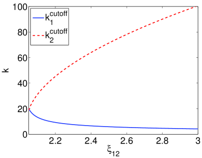
(a) Fixed $n^{0}=1$

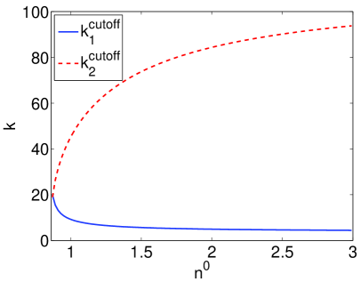
(b) Fixed $\xi_{12}=2.2$

Figure 1: Cutoff wave numbers as functions of $\xi_{12}$ with $n^{0}=1$ and as functions of $n^{0}$ with $\xi_{12}=2.2$.

When $\delta\rightarrow 0$, we have $k_{1}^{cutoff}\rightarrow\sqrt{-\frac{a}{b}}$ and $k_{2}^{cutoff}\rightarrow+\infty$. The unstable wave regime is $k>k_{1}^{cutoff}$. The system is unstable for large wave numbers (short waves), which is known as the Hadamard instability. Hence, the high order diffusion coefficients $\gamma_{1},\gamma_{2}$ have the effect to suppress the short wave instability.

This intermediate wave instability is also dependent of the constant state $n^{0}$. When the interaction parameter $\xi_{12}=2.2$ is fixed, but $n^{0}$ is varying, we find that $b$ is positive for small $n^{0}$ and negative for large $n^{0}$. That means the system is stable for dilute solution but unstable for rich solution. We also plot the cutoff wave numbers as functions of $n^{0}$ with fixed $\xi_{12}=2.2$ in Figure 1(b). The instability appears when $n^{0}>0.87$, and the unstable wave number regime $(k_{1}^{cutoff},k_{2}^{cutoff})$ widens as $n^{0}$ increases.

This intermediate wave instability is a feature of these three models. Through a numerical investigation, we confirm that this instability property can occur in all three models. In the following example (Figure 2), we use parameter values $N_{1}=N_{2}=1,\lambda_{1}=\lambda_{2}=0.02,\gamma_{1}=\gamma_{2}=10^{-4},\xi_{11}=\xi_{22}=1,\xi_{12}=2.2,n^{0}=1$ in the length scale $l_{0}=1nm$ regime. The instability condition (3.77) is satisfied. The two asymptotical cutoff wave numbers of EPNP model are $k_{1}^{cutoff}=9.24$ and $k_{2}^{cutoff}=45.23$, respectively, when length scale $l_{0}=1nm$. For the three models, the relation between the length scale and the growth rate follows a simple scaling law: we denote the two length scales as $l_{0}^{(1)},l_{0}^{(2)}$, the corresponding growth rates as $\alpha_{1}^{(1)},\alpha_{1}^{(2)}$, and the cutoff wave numbers as $k^{(1)},k^{(2)}$, respectively. If $\frac{l_{0}^{(2)}}{l_{0}^{(1)}}=K$, then the cutoff wave number ratio follows $\frac{k^{(2)}}{k^{(1)}}=K$ while the growth rate ratio follows $\frac{\alpha_{1}^{(2)}(Kk)}{\alpha_{1}^{(1)}(k)}=K^{2.5}$. This can be inferred from the definition of time scale $t_{0}=\sqrt{\frac{m_{0}l_{0}^{2}}{k_{B}T}}\sim l_{0}^{2.5},(m_{0}\sim l_{0}^{3})$. The numerical results in Figure 2 also confirm this analysis.

The analysis and numerical results show that the growth rates can be positive in some intermediate wave number regime depicted in Figure 2, instead of near the zero wave number range. In this case, the growth rate of the Full model is the smallest while the EPNP model’s is the highest. From the linear stability analysis, we notice that this instability is associated with a large interaction parameter $\xi_{12}$, a consequence of the finite size effect. A positive $\xi_{12}$ means that the interaction between different species due to their steric effects is repulsive. The analysis and numerical results tell us that the intermediate wave instability appears when the repulsive effect is sufficiently strong in the three models. This also can be obtained from the interaction free energy density $g$. The repulsive interaction due to the finite size effect is represented by $\frac{k_{B}T}{2}(\xi_{11}n_{1}^{2}+2\xi_{12}n_{1}n_{2}+\xi_{22}n_{2}^{2})$, which can be rewritten as $\frac{k_{B}T}{2}((\sqrt{\xi_{11}}n_{1}+\frac{\xi_{12}}{\sqrt{\xi_{11}}}n_{2})^{2}+(\xi_{22}-\frac{\xi_{12}^{2}}{\xi_{11}})n_{2}^{2})$. When $\xi_{12}$ is sufficiently large, $\xi_{11}\xi_{22}-\xi_{12}^{2}<0$, this quadratic form is hyperbolic type without lower bound. In the next nonlinear simulations, we only consider the cases $\xi_{11}\xi_{22}-\xi_{12}^{2}>0$, with out the intermediate wave instability.

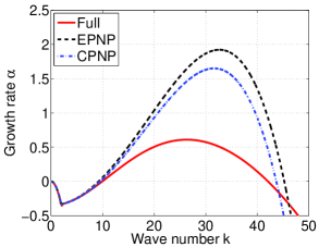
(a) $l_{0}=1nm.$

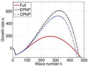
(b) $l_{0}=10nm.$

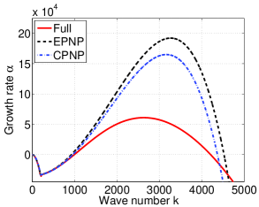
(c) $l_{0}=100nm.$

Figure 2: The growth rates of the full model and the two PNP models with length scale $l_{0}=1,10,100nm$, respectively, in the parameter regime of intermediate wave number instability. The values of growth rates increase as the length scale $l_{0}$ increases. The two cutoff wave numbers of the EPNP model in the length scale $l_{0}=1nm$ regime are $9.24$ and $45.23$, respectively. The full model is more stable than the other two models in this regime.

3.4.1 Discussion on the finite size effect

The hard sphere repulsion characterizes the finite-size effect of ions, witch keeps ions apart. The free energy density due to the finite-size effect is

$$\begin{array}[]{l}\int K({\bf x}-{\bf y})G(\{n_{i}\}_{i=1}^{N}({\bf x}),\{n_{i}\}_{i=1}^{N}({\bf y}))d{\bf y}=\int\sum_{i=1}^{N}\sum_{j=1}^{N}\frac{\varepsilon_{ij}}{2}\frac{(a_{i}+a_{j})^{12}}{|{\bf x}-{\bf y}|^{12}}n_{i}({\bf x})n_{j}({\bf y})d{\bf y},\end{array}$$ (3.82)

where $a_{i}$ and $a_{j}$ are the radii of ion $i$ and $j$, and $\varepsilon_{ij}$ is the energy coupling constant between ion $i$ and $j$. Thus, in the free energy function, we have the convolution integral with the following form

$$\begin{array}[]{l}\int\int\frac{1}{|{\bf x}-{\bf y}|^{12}}n_{i}({\bf x})n_{j}({\bf y})d{\bf y}d{\bf x}.\end{array}$$ (3.84)

We can approximate the above convolution integral by truncating the kernel $\frac{1}{|{\bf x}-{\bf y}|^{12}}$ with the cutoff length $\delta$. As discussed in the paper [69], when the cutoff length $\delta$ goes to zero, this convolution integral can be approximated by the integral

$$\begin{array}[]{l}S_{\delta}\int n_{i}({\bf x})n_{j}({\bf y})d{\bf x},\end{array}$$ (3.86)

with $S_{\delta}\approx\delta^{-12+d}$, where $d$ is the dimension. The free energy density due to the finite-size effect can be written as

$$\begin{array}[]{l}\sum_{i,j=1}^{N}\frac{\varepsilon_{ij}}{2}(a_{i}+a_{j})^{12}S_{\delta}n_{i}({\bf x})n_{j}({\bf x})=k_{B}T\sum_{i,j=1}^{N}\frac{\xi_{ij}}{2}n_{i}n_{j},\end{array}$$ (3.88)

with $\xi_{ij}=\frac{1}{k_{B}T}\varepsilon_{ij}(a_{i}+a_{j})^{12}S_{\delta}$. We add the conformational entropy in terms of the derivative form to compensate for the approximation error, then the energy density for the finite-size effect is approximated by

$$\begin{array}[]{l}g=k_{B}T[\sum_{i,j=1}^{N}\frac{\xi_{ij}}{2}n_{i}n_{j}+\sum_{i=1}^{N}\frac{\gamma_{i}}{2}\|\nabla n_{i}\|^{2}],\end{array}$$ (3.90)

where $\gamma_{i}$ is a small parameter, witch can be zero. In the paper [69], the following $\varepsilon_{ij}$ values for the cross hard-sphere potential terms for some familiar ions ($Na^{+},Cl^{-},Ca^{2+}$) are used:

$$\begin{array}[]{l}\varepsilon_{Na,Na}:\varepsilon_{Cl,Cl}:\varepsilon_{Ca,Ca}:\varepsilon_{Na,Cl}:\varepsilon_{Na,Ca}:\varepsilon_{Cl,Ca}=1:1:1:0.955:1:0.961.\end{array}$$ (3.92)

Also in the paper [69], the ratios of the interaction coefficients $\xi_{ij}$ are given for some familiar ions ($Na^{+},Cl^{-},Ca^{2+}$) as follows

$$\begin{array}[]{l}\xi_{Na,Na}:\xi_{Cl,Cl}:\xi_{Ca,Ca}:\xi_{Na,Cl}:\xi_{Na,Ca}:\xi_{Cl,Ca}=1:2280:1.64:42.2:0.642:50.4.\end{array}$$ (3.94)

It is easy to verify that $\xi_{11}\xi_{22}-\xi_{12}^{2}>0$ for two of the three ions. For the familiar ions, the interaction coefficients $\xi_{ij}$ are in the stable regime. That is the reason we only consider the stable cases in the nonlinear simulations next.

3.5 Nonlinear dynamics

We next explore nonlinear dynamics of the models in the linearly stable regime. We use the characteristic length scale $l_{0}=1nm$ and set the domain as $x\in[0,10]$. The values of the interaction parameters are chosen as $\xi_{11}=\xi_{22}=1,\xi_{12}=0.8$, satisfying $\xi_{11}\xi_{22}-\xi_{12}^{2}>0$. We also set diffusion coefficients $\gamma_{1}=\gamma_{2}=0$. The boundary conditions for the number densities $n_{1},n_{2}$ are no-flux boundary conditions (2.59); for the velocity ${\bf v}_{1}$, the boundary conditions are set at ${\bf v}_{1}|_{x=0,10}=0$, and for the electric potential $\Phi$, they are set at $\Phi|_{x=0}=0,\Phi|_{x=10}=\Phi_{0}$, where $\Phi_{0}$ is the electric potential at the right boundary $x=10$. We set $\Phi_{0}=1$ in the following simulations. The initial conditions are given by $n_{1}=n_{2}=n^{0}=1,\ {\bf v}_{1}=0,\ p=0,\ \Phi=\Phi_{0}x/10$. The given external electric potential is $\Phi_{e}=\Phi_{0}x/10$. The dimensionless mobilities are given as $\lambda_{1}=\lambda_{2}=0.02$. We compute the ionic number densities using the Full model, the EPNP model and the CPNP model, respectively.

Figures 3 depicts the final steady states of the Full model and the EPNP model, and the difference between them, where $\xi_{11}=\xi_{22}=1,\xi_{12}=0.8$ in the stable regime. The states of the number densities are almost identical in the middle of the domain, while the visible differences appear near the two boundaries. Because the electric potential is positive at the right boundary and zero at the left boundary, some negative ions gather at the right side while positive ions gather at the left side due to the Coulomb force, forming two visible boundary layers.

As shown in Figure 3, the density differences between the two models are about $O(1)\times 10^{-2}$ near the boundaries. As a conclusion, the compressibility of the flow in the full model plays relatively important role, it impacts the aggregation effect of the ions near the boundaries.

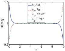
(a) Number density

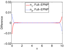
(b) Differences between the models

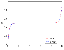
(c) Electric potential $\Phi$

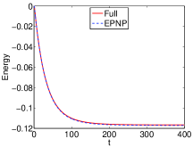
(d) Energy $F(t)-F(0)$

Figure 3: Steady states of the ionic densities and the electric potential of the Full and the EPNP models with $\xi_{11}=\xi_{22}=1,\xi_{12}=0.8$ in the stable regime, respectively. The differences appear near the boundary with absolute maximum difference $0.011$. The curve of energy difference $F(t)-F(0)$ is plotted with respect to time. The total free energy $F(t)$ decays to a constant when the final steady state is obtained.

In the above example, the density ratio is chosen as $\rho_{3}:\rho_{1}:\rho_{2}=1:0.5:2$. By halving density $\rho_{1}$ and doubling density $\rho_{2}$ to increase the density differences, we reset the density ratio as $\rho_{3}:\rho_{1}:\rho_{2}=1:0.25:4$ and $\rho_{3}:\rho_{1}:\rho_{2}=1:0.125:8$, while maintaining the volume ratio unchanged at $v_{3}:v_{1}:v_{2}=1:2:1$, then the dimensionless parameters are $R_{1}=0.0375,R_{2}=-0.075$ and $R_{1}=0.04375,R_{2}=-0.175$, respectively. In these cases, the size differences of the three components become larger. As shown in Figure 4, the differences between the Full model and the EPNP model become larger as the size differences become larger. When we halve the density $\rho_{1}$ and double the density $\rho_{2}$, the absolute maximum difference between the Full model and the EPNP model is almost doubled. As a result, when the size differences between the components are enlarged, the parameters $R_{1},R_{2}$ are no longer small so that the compressibility of the flow can no longer be neglected.

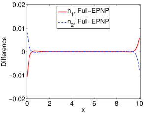
(a) $\rho_{3}:\rho_{1}:\rho_{2}=1:0.5:2$

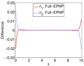
(b) $\rho_{3}:\rho_{1}:\rho_{2}=1:0.25:4$

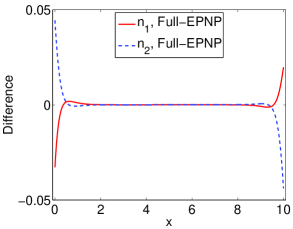
(c) $\rho_{3}:\rho_{1}:\rho_{2}=1:0.125:8$

Figure 4: Differences between the Full and the EPNP model with $\xi_{11}=\xi_{22}=1,\xi_{12}=0.8$ in the stable regime. (a) The density ratio is $\rho_{3}:\rho_{1}:\rho_{2}=1:0.5:2$ and $R_{1}=0.025,R_{2}=-0.025$, the absolute maximum difference is about $0.011$; (b) the density ratio is $\rho_{3}:\rho_{1}:\rho_{2}=1:0.25:4$ and $R_{1}=0.0375,R_{2}=-0.075$, the absolute maximum difference is about $0.022$; (c) the density ratio is $\rho_{3}:\rho_{1}:\rho_{2}=1:0.125:8$ and $R_{1}=0.04375,R_{2}=-0.175$, the absolute maximum difference is about $0.044$.

We also compare the EPNP and the CPNP model in the stable regime with $\xi_{11}=\xi_{22}=1,\xi_{12}=0.8$ in Figure 5. The density ratio $\rho_{3}:\rho_{1}:\rho_{2}=1:0.5:2$ is used. The values of the parameters are set at $r_{1}^{m}=1,r_{2}^{m}=2$. The number density differences between the two models are about $O(1)\times 10^{-2}$ near the boundaries. The differences near the boundaries in $n_{2}$ are bigger than that in $n_{1}$ . The reason is that in the CPNP model, the term $r_{i}^{m}\mu_{3}$ is dropped in the $n_{i}$ transport equation. In this example, $r_{2}^{m}>r_{1}^{m}$, so the differences near the boundaries of $n_{2}$ are bigger. Consequently, the solvent’s chemical potential $\mu_{3}$ in the EPNP model plays a relatively important role, it impacts the aggregation effect of the ions near the boundaries.

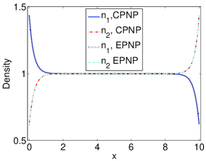
(a) Number density

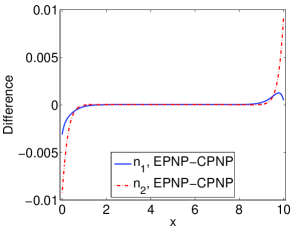
(b) Difference between the models

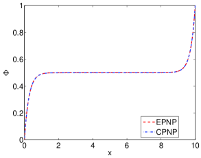
(c) Electric potential $\Phi$

Figure 5: Steady states of the ionic densities and electric potential of the EPNP and the CPNP model with $\xi_{11}=\xi_{22}=1,\xi_{12}=0.8$ in the stable regime. The difference appears at the boundary layers near both ends of the domain.

Next, we consider ionic concentrations without the finite size effect and compare them with ionic concentrations with the finite size effect using the classical PNP model. In the following, the OPNP means the classical PNP model without finite size effects (i.e., $\xi_{11}=\xi_{22}=\xi_{12}=0$ and $\gamma_{1}=\gamma_{2}=0$.) The differences also appear in the areas near the two boundaries. As shown in Figures 6, the differences of the ionic density can reach up to $O(1)\times 10^{-1}$. The finite size effect plays an important role in the system, it impacts the aggregation effect of the ions near the boundaries, as studied in the papers [26, 27, 33, 69].

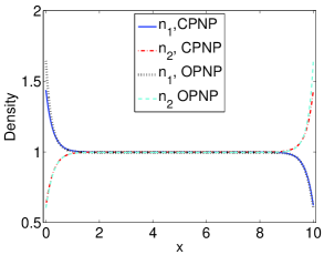
(a) Number density

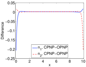
(b) Difference between the models

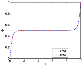
(c) Electric potential $\Phi$

Figure 6: Steady states of ionic densities and the electric potential of the CPNP and the OPNP model. In the CPNP model $\xi_{11}=\xi_{22}=1,\xi_{12}=0.8$ in the stable regime. The difference appears at the boundary layers near both ends of the domain.

Based on our numerical investigations and the linear analysis, we conclude that the 1D steady states of the number densities are nearly identical in the middle of the domain in all three models in the stable regime. The differences lie in the areas near the boundaries. The compressibility of the flow, the chemical potential of the solvent and the finite size effect are three main reasons that lead to the differences. So, our quasi-incompressible model (the full model) seems to be more reasonable because the mass and momentum conservation laws are preserved in the model while the other models don’t respect the two fundamental physical conservation laws.

Further investigations in higher dimensions is necessary to evaluate the difference among the models, which will be conducted in a sequel.

4 Conclusion

We have developed systematically a set of quasi-incompressible theories for ionic fluids of multiple species that respect not only momentum conservation but also mass conservation at the presence of the ionic species. The previous PNP type models are approximations of the more fundamental theories when densities of different ionic species are distinct. In these theories, we consider the entropic contribution from each ionic species together with the ion-ion interaction due to the finite size effect. The limiting cases include the extended PNP, the classical PNP with the finite size effect, and the classical PNP model without the finite size effect. At the length scale larger than hundreds of nanometers, all models agree with the classical PNP model very well. At the length scale in a few nanometers, the models can predict quite different stability behavior for homogeneous equilibrium states. In nonlinear dynamics, the ionic number densities are nearly identical in the middle of the domain, but the differences lie in the areas near the boundaries. Apparently, three main factors in the compressibility of the flow, the chemical potential of the solvent and the finite size effect of the ions can lead to the discrepancy in model predictions. We tend to believe that the new model is more accurate since it obeys the two fundamental physical conservation laws in mass and linear momentum while the others don’t.

Acknowledgment

Xiaogang Yang’s work is supported by the Scientific Research Fund of Wuhan Institute of Technology through Grants K201741; Jun Li’s work is partially supported by NSF of China through a grant (NSFC-11301287); Qi Wang is partially supported by NSF through awards DMS-1200487 and DMS-1517347 as well as a grant from NSFC # 11571032 and # 91630207.

5 Appendix

The linearized eigenvalue problem for the Full model is formulated as follows,

$$\left(\left(\begin{array}[]{ccccc}0&0&0&R_{1}\alpha&R_{2}\alpha\\ 0&0&0&0&0\\ 0&0&\rho_{k}\alpha&0&0\\ 0&0&0&\alpha&0\\ 0&0&0&0&\alpha\\ \end{array}\right)+\left(\begin{array}[]{ccccc}0&0&-ik\rho_{k}&0&0\\ 0&-k^{2}&0&\frac{1}{\varepsilon}&-\frac{1}{\varepsilon}\\ ik&0&(\frac{4}{3}\eta+\nu)k^{2}&B_{1}&B_{2}\\ R_{1}\lambda_{1}n^{0}k^{2}&\lambda_{1}n^{0}k^{2}&ikn^{0}&C_{1}&C_{2}\\ R_{2}\lambda_{2}n^{0}k^{2}&-\lambda_{2}n^{0}k^{2}&ikn^{0}&D_{1}&D_{2}\\ \end{array}\right)\right)\left(\begin{array}[]{c}p^{0}\\ \Phi^{0}\\ {\bf v}_{1}^{0}\\ n_{1}^{0}\\ n_{2}^{0}\\ \end{array}\right)=0,$$ (5.1)

where the parameter values are given by $n_{3}^{0}=r_{0}^{v}-r^{v}_{1}n^{0}-r^{v}_{2}n^{0}$ and $\rho_{k}=1-R_{1}n^{0}-R_{2}n^{0}$. The other components in the matrix are defined as follows

$$\begin{array}[]{l}B_{1}=-ikr_{1}^{v}+ikn^{0}(\frac{1}{N_{1}n^{0}}+\xi_{11}+\xi_{12})+ik^{3}n^{0}\gamma_{1},\\ B_{2}=-ikr_{2}^{v}+ikn^{0}(\frac{1}{N_{2}n^{0}}+\xi_{22}+\xi_{12})+ik^{3}n^{0}\gamma_{2},\\ C_{1}=\lambda_{1}n^{0}r_{1}^{m}r_{1}^{v}\frac{k^{2}}{n_{3}^{0}}+\lambda_{1}n^{0}(\frac{1}{N_{1}n^{0}}+\xi_{11})k^{2}+\lambda_{1}n^{0}\gamma_{1}k^{4},\\ C_{2}=\lambda_{1}n^{0}r_{1}^{m}r_{2}^{v}\frac{k^{2}}{n_{3}^{0}}+\lambda_{1}n^{0}(\xi_{12})k^{2},\\ D_{1}=\lambda_{2}n^{0}r_{2}^{m}r_{1}^{v}\frac{k^{2}}{n_{3}^{0}}+\lambda_{2}n^{0}(\xi_{12})k^{2},\\ D_{2}=\lambda_{2}n^{0}r_{2}^{m}r_{2}^{v}\frac{k^{2}}{n_{3}^{0}}+\lambda_{2}n^{0}(\frac{1}{N_{2}n^{0}}+\xi_{22})k^{2}+\lambda_{2}n^{0}\gamma_{2}k^{4}.\end{array}$$ (5.8)

Although the coefficient matrix is $5\times 5$, the characteristic polynomial of the coefficient matrix is a third order polynomial of growth rate $\alpha$, which yields three independent eigen-modes. Using an asymptotic analysis at small wave numbers $|k|\ll 1$, the three asymptotic growth rates are obtained asymptotically:

$$\begin{array}[]{l}\alpha_{1}=T_{1}k^{2}+O(k^{4}),\\ \\ \alpha_{2,3}=-\frac{T_{2}\pm\sqrt{T_{2}^{2}+T_{3}}}{T_{4}}+O(k^{2}),\end{array}$$ (5.12)

where

$$\begin{array}[]{l}T_{1}=-\frac{\lambda_{1}\lambda_{2}n^{0}}{(\lambda_{1}+\lambda_{2})n_{3}^{0}}[{\rho_{k}^{2}n_{3}^{0}}(\frac{1}{N_{1}n^{0}}+\frac{1}{N_{2}n^{0}}+\xi_{11}+\xi_{22}+2\xi_{12})+\rho_{k}(r_{1}^{v}+r_{2}^{v})((r_{1}^{m}+r_{2}^{m})+(R_{1}+R_{2})n_{3}^{0})],\\ \\ T_{2}=\lambda_{1}\lambda_{2}\rho_{k}(n^{0})^{2}(R_{1}+R_{2})^{2}+\varepsilon,\\ \\ T_{3}=-4(n^{0})^{2}\rho_{k}\varepsilon(\lambda_{1}+\lambda_{2})(\lambda_{1}R_{1}^{2}+\lambda_{2}R_{2}^{2}),\\ \\ T_{4}=2n^{0}\rho_{k}\varepsilon(\lambda_{1}R_{1}^{2}+\lambda_{2}R_{2}^{2}).\end{array}$$ (5.20)

Notice that $\alpha_{2,3}<0$ for small $k$ due to $T_{3}<0$. The eigenvalue $\alpha_{1}>0$ when $T_{1}>0$,

$$\begin{array}[]{l}\frac{1}{N_{1}n^{0}}+\frac{1}{N_{2}n^{0}}+\xi_{11}+\xi_{22}+2\xi_{12}<-\frac{r_{1}^{v}+r_{2}^{v}}{\rho_{k}n_{3}^{0}}((r_{1}^{m}+r_{2}^{m})+(R_{1}+R_{2})n_{3}^{0}).\end{array}$$ (5.22)

This is the instability condition for long waves for the Full model. It follows from eqn (3.69) that $(r_{1}^{m}+r_{2}^{m})+(R_{1}+R_{2})n_{3}^{0}>0$. So, the instability can incur only when $\xi_{11}+\xi_{22}+2\xi_{12}$ is negative enough. But, $\xi_{ij}>0$ in the model. So this mode of instability is absent from the full model.

For the EPNP model, only $n_{1},n_{2},\Phi$ are coupled, the eigenvalue problem is given by

$$\left(\left(\begin{array}[]{ccc}0&0&0\\ 0&\alpha&0\\ 0&0&\alpha\\ \end{array}\right)+\left(\begin{array}[]{ccc}-k^{2}&\frac{1}{\varepsilon}&-\frac{1}{\varepsilon}\\ \lambda_{1}n^{0}k^{2}&C_{1}&C_{2}\\ -\lambda_{2}n^{0}k^{2}&D_{1}&D_{2}\\ \end{array}\right)\right)\left(\begin{array}[]{c}\Phi^{0}\\ n_{1}^{0}\\ n_{2}^{0}\\ \end{array}\right)=0,$$ (5.23)

where

$$\begin{array}[]{l}C_{1}=\lambda_{1}n^{0}r_{1}^{m}r_{1}^{v}\frac{k^{2}}{n_{3}^{0}}+\lambda_{1}n^{0}(\frac{1}{N_{1}n^{0}}+\xi_{11})k^{2}+\lambda_{1}n^{0}\gamma_{1}k^{4},\quad C_{2}=\lambda_{1}n^{0}r_{1}^{m}r_{2}^{v}\frac{k^{2}}{n_{3}^{0}}+\lambda_{1}n^{0}\xi_{12}k^{2},\\ \\ D_{1}=\lambda_{2}n^{0}r_{2}^{m}r_{1}^{v}\frac{k^{2}}{n_{3}^{0}}+\lambda_{2}n^{0}\xi_{12}k^{2},\quad D_{2}=\lambda_{2}n^{0}r_{2}^{m}r_{2}^{v}\frac{k^{2}}{n_{3}^{0}}+\lambda_{2}n^{0}(\frac{1}{N_{2}n^{0}}+\xi_{22})k^{2}+\lambda_{2}n^{0}\gamma_{2}k^{4}.\end{array}$$ (5.27)

Eliminating $\Phi^{0}$, the system reduces to

$$\left(\left(\begin{array}[]{cc}\alpha&0\\ 0&\alpha\\ \end{array}\right)+\left(\begin{array}[]{cc}C_{1}+\lambda_{1}n^{0}\frac{1}{\varepsilon}&C_{2}-\lambda_{1}n^{0}\frac{1}{\varepsilon}\\ D_{1}-\lambda_{2}n^{0}\frac{1}{\varepsilon}&D_{2}+\lambda_{2}n^{0}\frac{1}{\varepsilon}\\ \end{array}\right)\right)\left(\begin{array}[]{c}n_{1}^{0}\\ n_{2}^{0}\\ \end{array}\right)=0,$$ (5.28)

The characteristic polynomial is quadratic and given by

$$\begin{array}[]{l}\alpha^{2}+[C_{1}+D_{2}+(\lambda_{1}+\lambda_{2})n^{0}\frac{1}{\varepsilon}]\alpha+A=0,\\ \\ A=C_{1}D_{2}-C_{2}D_{1}+[\lambda_{2}(C_{1}+C_{2})+\lambda_{1}(D_{1}+D_{2})]n^{0}\frac{1}{\varepsilon}.\end{array}$$ (5.32)

The two growth rates are given by

$$\begin{array}[]{l}\alpha_{1}=-2A\left[(C_{1}+D_{2}+(\lambda_{1}+\lambda_{2})n^{0}\frac{1}{\varepsilon})+\sqrt{(C_{1}+D_{2}+(\lambda_{1}+\lambda_{2})n^{0}\frac{1}{\varepsilon})^{2}-4A}\right]^{-1},\\ \\ \alpha_{2}=-\frac{1}{2}\left[(C_{1}+D_{2}+(\lambda_{1}+\lambda_{2})n^{0}\frac{1}{\varepsilon})+\sqrt{(C_{1}+D_{2}+(\lambda_{1}+\lambda_{2})n^{0}\frac{1}{\varepsilon})^{2}-4A}\right].\end{array}$$ (5.36)

Notice that $C_{1}\geq 0,D_{2}\geq 0$. So, $Re(\alpha_{2})<0$ and $Re(\alpha_{1})$ can be positive only if $A<0$.

References

- [1] Bird, Stewart, and Lightfoot, Transport Phenomena, John Wiley and Sons, 2002.
- [2] B. Bird, R. Armstrong, O. Hassager, Dynamics of Polymeric Liquids, 2nd Ed., Vol. 2, John Wiley and Sons, New York, 1987.
- [3] A. N. Beris and B. Edwards, Thermodynamics of Flowing Systems, Oxford University Press, Oxford, UK, 1994.
- [4] Boda, D., D. Henderson, A. Patrykiejew, and S. Sokolowski. Density Functional Study of a Simple Membrane Using the Solvent Primitive Model. J Colloid Interface Sci., 239 (2001), 432-439.
- [5] Burger, M., R. S. Eisenberg, and H. Engl. Inverse Problems Related to Ion Channel Selectivity. SIAM J Applied Math, 67 (2007), 960-989.
- [6] Burger, M. 2011. Inverse problems in ion channel modelling. Inverse Problems, 27 (2011), 083001.
- [7] J. W. Cahn and J. E. Hilliard. Free energy of a nonuniform system. i: interfacial free energy. J. Chem. Phys., 28 (1959), 258–267.
- [8] J. W. Cahn and J. E. Hilliard. Free energy of a nonuniform system-iii: Nucleation in a 2-component incompressible fluid. J. Chem. Phys., 31(3) (1959), 688–699.
- [9] L. Q. Chen and W. Yang, Computer simulation of the dynamics of a quenched system with large number of non-conserved order parameters, Phys. Rev. B, 50 (1994), 15752-15756.
- [10] L. Q. Chen, Phase-field modeling for microstructure evolution, Annu. Rev. Mater. Res., 32 (2002), 113-140.
- [11] L. Q. Chen and Y. Wang, The Continuum Field Approach to Modeling Microstructural Evolution, J. Miner Met. Mater. Soc., 48 (12) (1996), 13-18.
- [12] M. Doi, Introduction to Polymer Physics, Clarendon Press, Oxford, UK, 1996.
- [13] Q. Du, C. Liu, R. Ryham and X. Wang, Phase field modeling of the spontaneous curvature effect in cell membranes, Comm. Pur. Applied. Anal., 4 (2005), 537-548.
- [14] Q. Du, C. Liu and X. Wang, A Phase Field Approach in the Numerical Study of the Elastic Bending Energy for Vesicle Membranes, J. Comp. Phy., 198 (2004), 450-468.
- [15] R.S. Eisenberg, Computing the field in proteins and channels, J. Membrane Biol., 150 (1996), 1-25.
- [16] R. S. Eisenberg, Ionic channels in biological membranes: electrostatic analysis of a natural nano-tube, Contemp. Phys., 39 (1998), 447-466.
- [17] M. G. Forest and Q. Wang, Hydrodynamic theories for blends of flexible polymer and nematic polymers, Physical Review E, 72 (2005), 041805.
- [18] M. G. Forest, Q. Liao and Qi Wang, 2-D Kinetic Theory for Polymer Particulate Nanocomposites, Communication in Computational Physics, 7 (2) (2010), 250-282.
- [19] J. J. Feng, C. Liu, J. Shen and P. Yue, Transient Drop Deformation upon Startup of Shear in Viscoelastic Fluids, Fluids. Phys. Fluids, 17 (2005), 123101.
- [20] P. J. Flory, Principles of Polymer Chemistry, Cornell University Press, Ithaca, NY, 1953.
- [21] R. Hobayashi, Modeling and numerical simulations of dendritic crystal growth, Physica D, 63 (1993), 410-423.
- [22] U. Hollerbach, D.P. Chen, D. D. Busath, and R. S. Eisenberg, Predicting function from structure using the Poisson-Nernst-Planck equations: sodium current in the gramicidin A channel, Langmuir, 16 (2000), 5509-5514.
- [23] U. Hollerbach, D.P. Chen, and R.S. Eisenberg, Two and Three Dimensional Poisson-Nernst-Planck Simulations of Current Through Gramicidin-A, J. Scientific Computing, 16 (4) (2001), 373-409.
- [24] Fitzhugh, R. 1983. Statistical properties of the asymmetric random telegraph signal, with applications to single-channel analysis. Mathematical Biosciences, 64 (1983), 75-89.
- [25] Jinsong Hua, Ping Lin, Chun, Liu, Qi Wang, Energy Law Preserving Finite Element Schemes for Phase Field Models in Two-phase Flow Computations, J. Comp. Phys., 230 (19) (2011), 7115-7131.
- [26] Y. Hyon, R. Eisenberg and C. Liu, A Mathematical Model for the Hard Sphere Resulsion in Ionic Solutions, Commum. Math. Sci., Vol. 9, No. 2 (2011), 459-475.
- [27] Y. Hyon, R. Eisenberg and C. Liu, An energetic variational approach to ion channel dynamics, Mathematical Methods in the Applied Sciences, Vol. 37, no.7 (2014), 952-961.
- [28] A. Karma and W. Rappel, Phase-Field Model of Dendritic Sidebranching with Thermal Noise, Phys. Rev. E, 60 (1999), 3614-3625.
- [29] Lamperski, S., and A. Zydor. Monte Carlo study of the electrode—solvent primitive model electrolyte interface. Electrochimica Acta, 52 (2007), 2429-2436.
- [30] Lee, J. W., J. A. Templeton, K. K. Mandadapu, and J. A. Zimmerman. Comparison of Molecular and Primitive Solvent Models for Electrical Double Layers in Nanochannels. Journal of Chemical Theory and Computation, 9 (2013), 3051-3061.
- [31] Jun Li and Qi Wang, Mass Conservation and Energy Dissipation Issue in a Class of Phase Field Models for Multiphase Fluids, Journal of Applied Mechanics, 81(2), 2013, 021004.
- [32] B. Lindley, Q. Wang and T. Zhang, Multicomponent models for biofilm flows, Discrete and Continuous Dynamic Systems- Series B,15(2) (2011), 417-456.
- [33] T.-C. Lin and R. Eisenberg. Multiple solutions of steady-state Poisson-Nernst-Planck equations with steric effects, nonlinearity, Vol. 28(7) (2015), 103-127.
- [34] C. Liu and N. J. Walkington, An Eulerian description of fluids containing visco-hyperelastic particles, Arch. Rat. Mech. Ana., 159 (2001), 229-252.
- [35] C. Liu and J. Shen, A phase field model for the mixture of two incompressible fluids and its approximation by a fourier-spectral method, Physica D, 179 (2003), 211-228.
- [36] Y. Li, S. Hu, Z. Liu, and L. Chen, Phase-field model of domain structures in ferroelectric thin films, Appl. Phys. Lett., 78 (2001), 3878-3880.
- [37] W. Lu and Z. Suo, Dynamics of nanoscale pattern formation of an epitaxial monolayer, J. Mech. Phys. Solids, 49 (2001), 1937-1950.
- [38] J. Lowengrub and L.Truskinovsky, Quasi-incompressible Cahn-Hilliard fluids and topological transitions, R. Soc. Lond. Proc. Ser. A Math. Phys. Eng. Sci., 454 (1998), 2617–2654.
- [39] P. M. Chaikin and T. C. Lubensky, Principles of Condense Matter Physics, Cambridge University Press, Cambridge, UK, 1995.
- [40] G. McFadden, A. Wheeler, R. Braun, S. Coriell, and R. Sekerka, Phys. Rev. E, 48 (1998), 2016-2024.
- [41] Neher, E. Ion channels for communication between and within cells Nobel Lecture, December 9, 1991. In Nobel Lectures, Physiology or Medicine 1991-1995. N. Ringertz, editor. World Scientific Publishing Co, Singapore. 1997, 10-25.
- [42] Probstein, Physicochemical Hydrodynamics, John Wiley and Sons, 1994.
- [43] Rosenfeld, Y., M. Schmidt, H. Lowen, and P. Tarazona. Fundamental-measure free-energy density functional for hard spheres: Dimensional crossover and freezing. Physical Review E, 55 (1997), 4245-4263.
- [44] Rosenfeld, Y. Self-consistent density functional theory and the equation of state for simple fluids. Molecular Physics, 94 (1998), 929-935.
- [45] D. J. Seol, S. Y. Hu, Y. L. Li, J. Shen, K. H. Oh and L. Q. Chen, Three-dimensional Phase-Field Modeling of Spinodal Decomposition in Constrained Films, Acta Materialia, 51 (2003), 5173-5185.
- [46] J. Shen and X. Yang, An efficient moving mesh spectral method for the phase-field model of two phase flows, J. Comput. Phys., 228 (2009), 2978-2992.
- [47] J. Shen and X. Yang, Energy Stable Schemes for Cahn-Hilliard phase-field model of two-phase incompressible flows, Chinese Ann. Math. series B, 31 (2010), 743-758.
- [48] J. Shen and X. Yang, A phase-field model and its numerical approximation for two-phase incompressible flows with different densities and viscositites, SIAM J. Sci. Comput., 32(3) (2010), 1159-1179.
- [49] E. Tadmor, R. Phillips, and M. Ortiz, Mixed Atomistic and Continuum Models of Deformation in Solids, Langmuir, 12 (1996), 4529-4534.
- [50] Tang, Y. W., I. Szalai, and K.-Y. Chan. Diffusivity and conductivity of a solvent primitive model electrolyte in a nanopore by equilibrium and nonequilibrium molecular dynamics simulations. The Journal of Physical Chemistry A, 105 (2001), 9616-9623.
- [51] T. A. van der Straaten, J. Tang, R. S. Eisenberg, U. Ravaioli, and N. R. Aluru, Three-dimensional continuum simulations of ion transport through biological ion channels: eÆects of charge distribution in the constriction region of porin, J. Computational Electronics, 1 (2002), 335-340.
- [52] Q. Wang, W. E, C. Liu, and P. Zhang, Kinetic theories for flows of nonhomogeneous rodlike liquid crystalline polymers with a nonlocal intermolecular potential, Physical Review E, 65(5) (2002), 0515041-0515047.
- [53] Q. Wang, A hydrodynamic theory of nematic liquid crystalline polymers of different configurations, Journal of Chemical Physics, 116 (2002), 9120-9136.
- [54] Q. Wang, M. G. Forest and R. Zhou, A hydrodynamic theory for solutions of nonhomogeneous nematic liquid crystalline polymers with density variations, J. of Fluid Engineering, 126 (2004), 180-188.
- [55] Q. Wang and T. Y. Zhang, Kinetic theories for Biofilms, Discrete and Continuous Dynamic Systems - Series B, 17 (3) (2012), 1027-1059.
- [56] Y. Wang and C. L. Chen, Simulation of microstructure evolution. In Methods in Materials Research, Ed. E. N. Ksufmann, R. Abbaschian, A. Bocarsly, C. L. Chien, D. Dollimore, et al., (1999), 2a3.1-2a3.23.
- [57] A. Wheeler, G. McFadden, and W. Boettinger, Proc. R. Soc. London Ser. A, 452 (1996), 495-525.
- [58] S. M. Wise, J. S. Lowengrub, J. S. Kim and W. C. Johnson, Efficient phase-field simulation of quantum dot formation in a strained heteroepitaxial film, Superlattices and Microstructures, 36 (2004) 293-304.
- [59] X. Yang, J. Feng, C. Liu and J. Shen, Numerical simulations of jet pinching-off and drop formation using an energetic variational phase-field method, J. Comput. Phys., 218 (2006), 417-428.
- [60] Xiaogang Yang, M. G. Forest, and Qi Wang, Near Equilibrium Dynamics and 1-D Spatial-Temporal Structures of Polar Active Liquid Crystals, Chinese Phys. B, 23(11) (2014),117502.
- [61] P. Yue, J. J. Feng, C. Liu, and J. Shen, A diffuse-interface method for simulating two-phase flows of complex fluids, J. Fluid Mech., 515 (2004), 293–317.
- [62] P. Yue, J. J. Feng, C. Liu, and J. Shen, Diffuse-interface simulations of drop coalescence and retraction in viscoelastic fluids, J. Non-Newtonian Fluid Mech., 129 (2005), 163-176.
- [63] T. Y. Zhang, N. Cogan, and Q. Wang, Phase Field Models for Biofilms. II. 2-D Numerical Simulations of Biofilm-Flow Interaction, Communications in Computational Physics, 4 (2008), 72-101.
- [64] T. Y. Zhang and Q. Wang, Cahn-Hilliard vs Singular Cahn-Hilliard Equations in Phase Field Modeling, Communication In CP, 7(2) (2010), 362-382.
- [65] Jia Zhao, Ya Shen, Markus Haapasalo, Zhejun Wang, and Qi Wang, A 3D Numerical Study of Antimicrobial Persistence in Heterogeneous Multi-species Biofilms. Journal of Theoretical Biology, 392, (2016), 8398.
- [66] Jia Zhao and Qi Wang, A 3D Multi-Phase Hydrodynamic Model for Cytokinesis of Eukaryotic Cells, Communication in Computational Physics, 19(03) (2016), 663-681.
- [67] Jia Zhao and Qi Wang, Modeling cytokinesis of eukaryotic cells driven by the actomyosin contractile ring, International Journal for Numerical Methods in Biomedical Engineering, (2016), e02774.
- [68] Zheng, J., and M. C. Trudeau. Handbook of ion channels. CRC Press, 2015.
- [69] Tzyy-Leng Horng, Tai-Chia Lin, Chun Liu and Bob Eisenberg. PNP Equations with Steric Effects: A Model of Ion Flow through Channels. Jouranl of Physical Chemistry B, 116(37), (2012), 11422.
- [70] Jun Li and Qi Wang. A Class of Conservative Phase Field Models for Multiphase Fluid Flows. Journal of Applied Mechanics, 81(2), (2014), 021004.