Quantifying Uncertainty in High Dimensional Inverse Problems by Convex Optimisation

Abstract

Inverse problems play a key role in modern image/signal processing methods. However, since they are generally ill-conditioned or ill-posed due to lack of observations, their solutions may have significant intrinsic uncertainty. Analysing and quantifying this uncertainty is very challenging, particularly in high-dimensional problems and problems with non-smooth objective functionals (e.g. sparsity-promoting priors). In this article, a series of strategies to visualise this uncertainty are presented, e.g. highest posterior density credible regions, and local credible intervals (cf. error bars) for individual pixels and superpixels. Our methods support non-smooth priors for inverse problems and can be scaled to high-dimensional settings. Moreover, we present strategies to automatically set regularisation parameters so that the proposed uncertainty quantification (UQ) strategies become much easier to use. Also, different kinds of dictionaries (complete and over-complete) are used to represent the image/signal and their performance in the proposed UQ methodology is investigated.

I Introduction

Inverse problems, like reconstruction (e.g. [1, 2]), denosing (e.g. [3]) or deblurring (e.g. [4]), are important subjects in image/signal processing. Briefly speaking, the task is to recover images/signals that are as close to natural ones as possible from corrupted observations, e.g. noisy, blurry and/or incomplete data. The degraded quality of the observations makes the associated inverse problems ill-conditioned or ill-posed, and therefore their solutions may have significantly intrinsic uncertainty (see e.g. [5, 6]). Quantifying this kind of uncertainty, particularly for high-dimensional problems, is very challenging. This is the main focus in this article.

Briefly speaking, inverse problems in image/signal processing can be generally formulated as regularised estimation problems involving a data fidelity term and a regularisation term, which are often substantiated by using a statistical likelihood function and a prior distribution, respectively (see Section II for more detail). Statistical sampling approaches like Markov Chain Monte Carlo (MCMC) sampling can in principle recover the full posterior probability distribution of the image/signal from the given inverse problems, from which uncertainties (like error bars) can then be quantified, see e.g. [5, 6, 7, 8]. However, due to the long computation time required to sample the full posterior distribution, these kind of methods can be extremely slow when data sets are large. As an alternative, maximum a posteriori (MAP) estimation has been adopted as a standard approach, combined with convex optimisation techniques to compute the estimator in practice [9, 10]. Such approaches have led to significant improvements in estimation accuracy and computation time in high dimensional scenarios. Recently, the authors proposed a series of uncertainty quantification (UQ) strategies based on MAP estimation [11] to visualise uncertainties [5, 12], illustrated for radio interferometric (RI) imaging. Note that the UQ techniques presented in [11, 12], which possess the advantages of MAP estimation as mentioned above, are very different to the methods using MCMC sampling [5, 6, 7] but accurately approximate the same forms of UQ (see [5, 6, 7, 11, 12] for more details).

In this article, based on the high-posterior-density (HPD) region approximation method [11], we develop strategies to efficiently perform UQ in general image/signal processing inverse problems. In particular, general dictionaries are considered in prior knowledge, and the involved regularisation parameter, which controls the strength of the prior knowledge in inverse problems and plays a key role in UQ analyses, is estimated automatically and used for the subsequent UQ analyses. Simulations are implemented to demonstrate the validity and effectiveness of the UQ strategies in terms of computing local credible intervals (cf. error bars or Bayesian confidence intervals) for individual pixels and superpixels.

II Problem Formulation

Let $\bm{y}\in\mathbb{C}^{M}$ represent the observed data set (an image/signal degraded and/or transformed by some operators [e.g. Fourier transform, blur operator], noise, and/or information loss), which satisfies ${\bm{y}}=\bm{\mathsf{\Phi}}{\bm{x}}+{\bm{n}}$, where $\bm{\mathsf{\Phi}}\in\mathbb{C}^{M\times N}$, ${\bm{x}}\in\mathbb{R}^{N}$, and ${\bm{n}}\in\mathbb{C}^{M}$ denote, respectively, a problem related operator, the clean image/signal, and noise. Without loss of generality, we subsequently consider independent and identically distributed (i.i.d.) Gaussian noise. Under a basis or dictionary (e.g., a wavelet basis or an over-complete frame [13]) $\bm{\mathsf{\bm{\mathsf{\Psi}}}}\in\mathbb{C}^{N\times L}$, $\bm{x}$ can be represented by ${\bm{x}}=\bm{\mathsf{\Psi}}{\bm{a}}=\sum_{i}\bm{\mathsf{\Psi}}_{i}a_{i}$, where vector ${\bm{a}}=(a_{1},\cdots,a_{L})^{\top}$ represents the synthesis coefficients of ${\bm{x}}$ under $\bm{\mathsf{\Psi}}$. In particular, ${\bm{x}}$ is said to be compressible if many coefficients of $\bm{a}$ are small; natural images are generally compressible for appropriate choices of $\bm{\mathsf{\Psi}}$ [14].

In practice, $\bm{y}$ is only observed partially or with limited resolution and thus solving

$${\bm{y}}=\bm{\mathsf{\Phi}}\bm{x}+{\bm{n}}\quad{\rm or}\quad{\bm{y}}=\bm{\mathsf{\Phi}}\bm{\mathsf{\Psi}}{\bm{a}}+{\bm{n}}$$ (1)

for $\bm{x}$ presents an ill-posed inverse problem. In particular, when $\bm{\mathsf{\Phi}}$ is an identity operator, blur operator (e.g., Gaussian), or transformation (e.g., Fourier or Radon), the above inverse problem goes to image/signal denosing, deblurring, or reconstruction, respectively (see e.g. [15, 5, 3, 16, 9] for more detail).

Bayesian inference. Estimating $\bm{x}$ (or $\bm{a}$) in problem (1) can be addressed in the Bayesian statistical framework [8]. Using Bayes’ theorem we obtain the posterior distribution

$$p(\bm{x}|\bm{y})={p(\bm{y}|\bm{x})p(\bm{x})}/{\int_{\mathbb{R}^{N}}p(\bm{y}|\bm{x})p(\bm{x}){\rm d}\bm{x}},$$ (2)

which models our knowledge about $\bm{x}$ after observing $\bm{y}$ given prior information, and where $p(\bm{y}|\bm{x})$ and $p(\bm{x})$ respectively represent the likelihood function and prior distribution (used to regularise the original problem, reduce uncertainty, and improve estimation results) of $\bm{x}$. Using Bayes’ theorem to model $\bm{a}$, $p(\bm{a}|\bm{y})$ is given analogously. The general forms of the likelihood function and prior distribution considered are $p(\bm{y}|\bm{x})\propto{\rm exp}(-g_{\bm{y}}(\bm{x}))$ and $p(\bm{x})\propto{\rm exp}(-\mu f(\bm{x}))$, respectively, where $\mu$ represents the so-called regularisation parameter which controls the strength of the prior information. The classical forms used are $g_{\bm{y}}(\bm{x})=\|\bm{y}-\bm{\mathsf{\Phi}}\bm{x}\|_{q}^{q}/2\sigma^{2}$, $f(\bm{x})=\|\bm{\mathsf{\Psi}}^{\dagger}\bm{x}\|_{s}$, where $q,s\geq 0$ (often $s=1$ is used), and $\sigma$ represents the standard deviation of the noise level.

MAP estimation. Sampling the full posterior $p(\bm{x}|\bm{y})$ or $p(\bm{a}|\bm{y})$ by e.g. MCMC methods is difficult when high dimensionality is involved [5, 12, 7, 6, 17]. Instead, Bayesian estimators that summarise $p(\bm{x}|\bm{y})$ or $p(\bm{a}|\bm{y})$ are often computed. A particularly popular choice is the MAP estimator, given by

$${\bm{x}}^{*}_{\mu}=\mathop{\rm argmin}_{\bm{x}\in\mathbb{R}^{N}}\big{\{}\mu f(\bm{x})+g_{\bm{y}}(\bm{x})\big{\}}.$$ (3)

In the rest of this article we assume $f(\bm{x})$ and $g_{\bm{y}}(\bm{x})$ are closed convex functions which are not necessarily differentiable, and the objective functional (3) is computationally tractable with respect to $\bm{x}$ given the value of $\mu$. For further details about MAP estimation see, e.g., [18].

A main computational advantage of the MAP estimator (3) is that it can be computed very efficiently, even in high dimensions, by using convex optimisation algorithms (e.g. [10, 9, 19]). However, since MAP estimation results in a single point estimator, we lose uncertainty information that sampling approaches like MCMC methods can provide [5]. But as shown in [11], it is possible to approximately quantify the uncertainties associated with $\bm{x} |\bm{y}$ by leveraging recent results in the theory of probability concentration.

Optimisation algorithms. There are many convex minimisation methods that can be used to solve the MAP estimation problems with form (3) efficiently, such as forward-backward splitting, Douglas-Rachford splitting, primal-dual, or alternating direction method of multipliers (see [10, 20, 21] and references therein for more detail). Furthermore, algorithmic structures that allow computations to be highly distributed and parallelised have also been developed, see e.g. [22, 23, 24, 21]. Note that to solve problem (3), the regularisation parameter $\mu$ should either be given beforehand or be estimated from $\bm{y}$.

Selecting the value of the regularisation parameter $\mu$ in (3) correctly is crucial, as this value impacts strongly the estimation results [25]. Setting appropriate values for $\mu$ by hand is generally difficult, and fortunately there are now several different kinds of Bayesian and non-Bayesian methods to select $\mu$ automatically [25, 26, 27, 28]. In the following, we briefly recall the Bayesian method [25] (coming from a hierarchical Bayesian model and using joint MAP estimation), which we adopt for our UQ strategies. The resulting iteration formula is given by

$$\begin{split}{\bm{x}}^{(i)}&=\mathop{\rm argmin}_{\bm{x}\in\mathbb{R}^{N}}\big{\{}\mu^{(i-1)}f(\bm{x})+g_{\bm{y}}(\bm{x})\big{\}},\\ \mu^{(i)}&=(N/k+\gamma-1)/(f({\bm{x}}^{(i)})+\beta),\end{split}$$ (4)

where $\gamma,\beta$ are fixed parameters (default values are 1), and $k$ is related to the definition of $f$ and is fixed as well (e.g. $k=1$ when $f$ is $\ell_{1}$ norm); refer to [25] for more detail.

III Proposed Uncertainty Quantification Methods

As discussed previously, MCMC methods sampling the full posterior $p(\bm{x}|\bm{y})$ [or $p(\bm{a}|\bm{y})$] to quantify uncertainties is computationally expensive when high dimensionality is involved. Instead, Bayesian credible regions can be estimated approximately based on the MAP estimator that summarises $p(\bm{x}|\bm{y})$ [or $p(\bm{a}|\bm{y})$], which does scale efficiently to high-dimensional settings [11, 12].

The diagram in Fig. III shows the main procedures of our proposed UQ methodology based on MAP estimation. Firstly, the objective functional related to a given inverse problem is formed, followed by estimation of $\mu$ (e.g. using the method in [25], shown in (4)) and MAP estimation of $\bm{x}$ using convex optimisation techniques (which can scale to high-dimensional problems where MCMC methods struggle). Then, various forms of UQ, e.g. those described in [12], are performed. Here we restrict our attention on local credible interval at pixel level (cf. error bars).

Figure 1: UQ methodology based on MAP estimation for image/signal processing. The light green areas at the bottom show the types of UQ developed.

The first step in our UQ pipeline is to compute the HPD region $C_{\alpha}$ with level $(1-\alpha)$, defined by $C_{\alpha}:=\{\bm{x}:\mu f(\bm{x})+g_{\bm{y}}(\bm{x})\leq\gamma_{\alpha}\}$ [8], with $\gamma_{\alpha}$ such that

$$p(\bm{x}\in C_{\alpha}|\bm{y})=\int_{\bm{x}\in\mathbb{R}^{N}}p(\bm{x}|\bm{y})\mathbb{1}_{C_{\alpha}}{\rm d}\bm{x}=1-\alpha\,.$$ (5)

Computing $C_{\alpha}$ exactly is often not possible when $N=\textrm{dim}(\bm{x})$ is large. However, from [11], we can have an approximation of $C_{\alpha}$, say $C^{\prime}_{\alpha}$, obtained by approximating $\gamma_{\alpha}$ by $\gamma^{\prime}_{\alpha}$ given by

$${\gamma}^{\prime}_{\alpha}=\mu f({\bm{x}}^{*}_{\mu})+g_{\bm{y}}({\bm{x}}^{*}_{\mu})+\sqrt{16\log(3/\alpha)}\sqrt{N}+N.$$ (6)

This approximation was motivated from recent results in information theory in terms of a probability concentration inequality, and is generally accurate for large $N$ (refer to [11, 12] for more details).

The second step in the pipeline is to use $C^{\prime}_{\alpha}$ to compute local credible interval for pixels and superpixels. This is a form of Bayesian UQ that we use as a means for visualising uncertainty spatially at different scales [12]. Let $\Omega=\cup_{i}\Omega_{i}$ be a partition of the image/signal domain $\Omega$ into subsets or superpixels $\Omega_{i}$ satisfying $\Omega_{i}\cap\Omega_{j}=\emptyset,i\neq j$. Then a local credible interval $({\xi}_{-,\Omega_{i}},{\xi}_{+,\Omega_{i}})$ for region $\Omega_{i}$ is defined by

$${\xi}_{-,\Omega_{i}} \!=\!\min_{\xi}\left\{\xi|\mu f({\bm{x}}_{i,\xi})\!+\!g_{\bm{y}}({\bm{x}}_{i,\xi})\leq{\gamma}^{\prime}_{\alpha},\forall\xi\in[0,+\infty)\right\},$$ (7)

$${\xi}_{+,\Omega_{i}} \!=\!\max_{\xi}\left\{\xi|\mu f({\bm{x}}_{i,\xi})\!+\!g_{\bm{y}}({\bm{x}}_{i,\xi})\leq{\gamma}^{\prime}_{\alpha},\forall\xi\in[0,+\infty)\right\},$$ (8)

where ${\bm{x}}_{i,\xi}={\bm{x}}_{\mu}^{*}\bm{\zeta}_{\Omega\setminus\Omega_{i}}+\xi\bm{\zeta}_{\Omega_{i}}$, $\bm{\zeta}_{\Omega_{i}}\in\mathbb{R}^{N}$ is the index operator on $\Omega_{i}$ with value 1 for pixels in $\Omega_{i}$ otherwise 0. Note that ${\xi}_{-,\Omega_{i}}$ and ${\xi}_{+,\Omega_{i}}$ are actually the values that saturate the HPD credible region $C^{\prime}_{\alpha}$ from above and from below at $\Omega_{i}$. Then the local credible interval $({\bm{\xi}}_{-},{\bm{\xi}}_{+})$ for the whole image/signal is obtained by gathering all the $({\xi}_{-,\Omega_{i}},{\xi}_{+,\Omega_{i}}),\forall i$, i.e.,

$${\bm{\xi}}_{-}=\sum_{i}{\xi}_{-,\Omega_{i}}\bm{\zeta}_{\Omega_{i}},\quad{\bm{\xi}}_{+}=\sum_{i}{\xi}_{+,\Omega_{i}}\bm{\zeta}_{\Omega_{i}}.$$ (9)

We hereby briefly clarify the distinctions of this work from [12]. Firstly, we now concern the UQ strategies in general image/signal processing problems instead of just a special application in RI imaging in [12]. Secondly, here we adjust $\mu$ automatically, but [12] assumes $\mu$ is known beforehand. Finally, we consider the over-complete bases $\bm{\mathsf{\bm{\mathsf{\Psi}}}}$ (such as SARA [13, 29]) and explore their influence in UQ with synthesis and analysis priors, which is not considered in [12].

IV Experiments

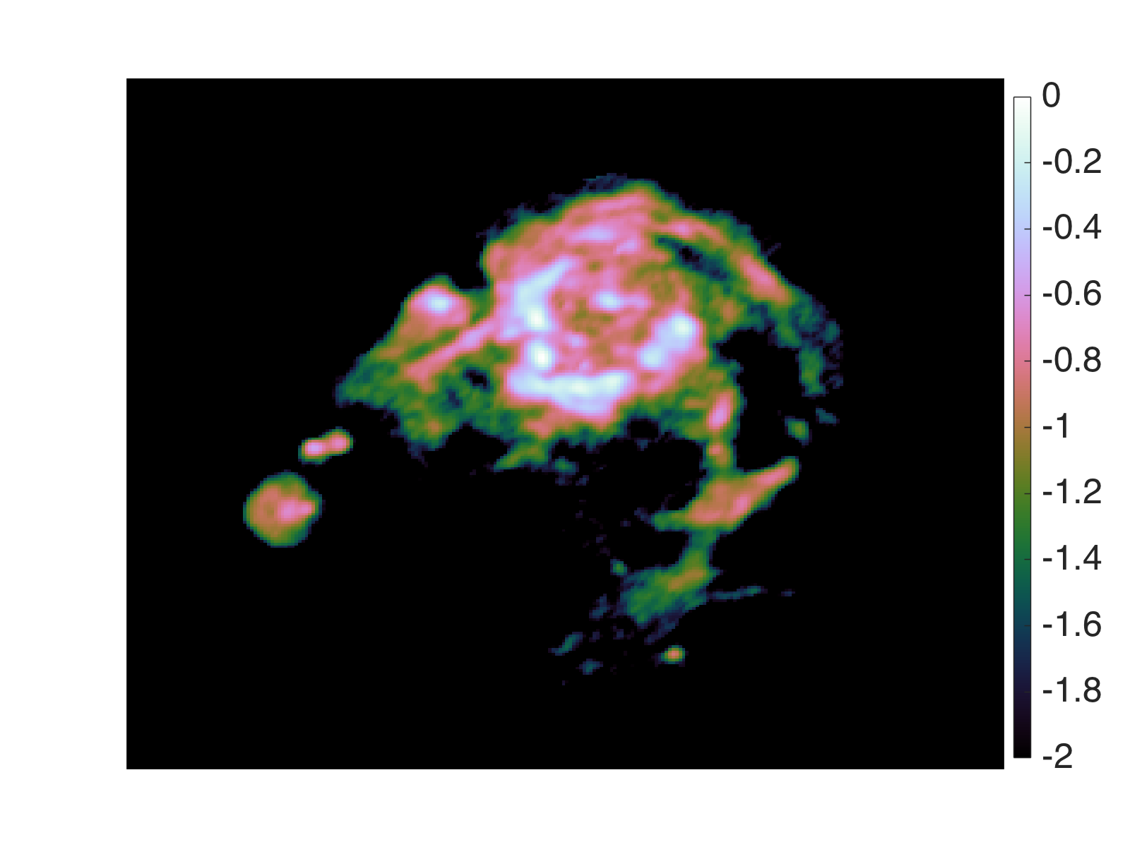
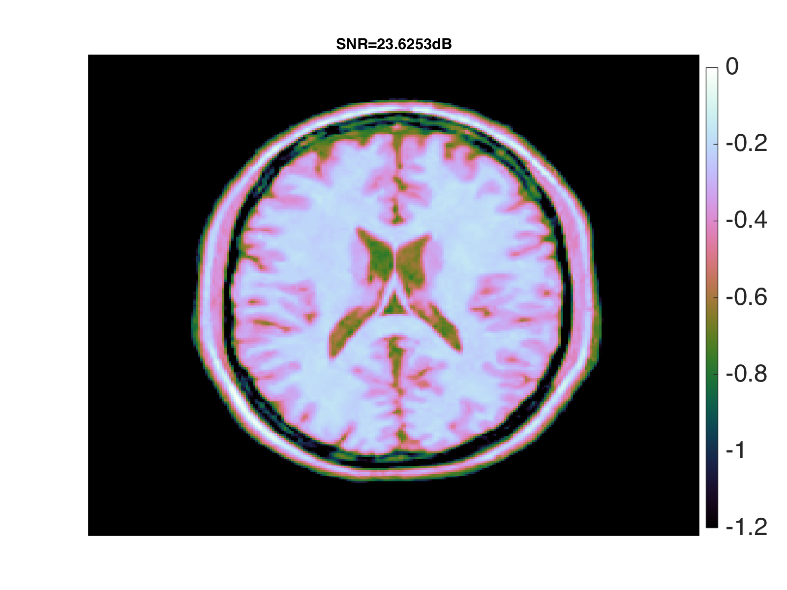
Figure 2: Test images in applications of RI imaging and medical imaging; shown in ${\tt log}_{10}$ scale. Left: RI image M31; right: MRI brain image.

TABLE I: Reconstruction quality in SNR and the automatically computed parameter $\mu$ with orthonormal basis and SARA library, corresponding to synthesis and analysis priors.

Image	Library/basis	Synthesis	Analysis	$\mu$
M31	Orthonormal	$25.04$	$25.04$	196
	SARA	$23.66$	$31.09$	65
Brain	Orthonormal	$19.06$	$19.06$	33
	SARA	$19.89$	$23.63$	11

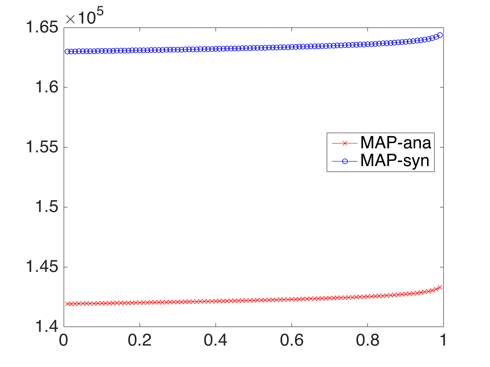
Figure 3: HPD credible region. Plots on the left and right are the results using orthonormal basis and SARA dictionary, respectively. MRI brain image is used as an example here (results for RI image M31 are similar).

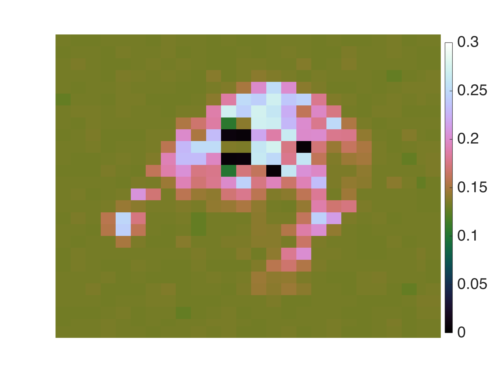
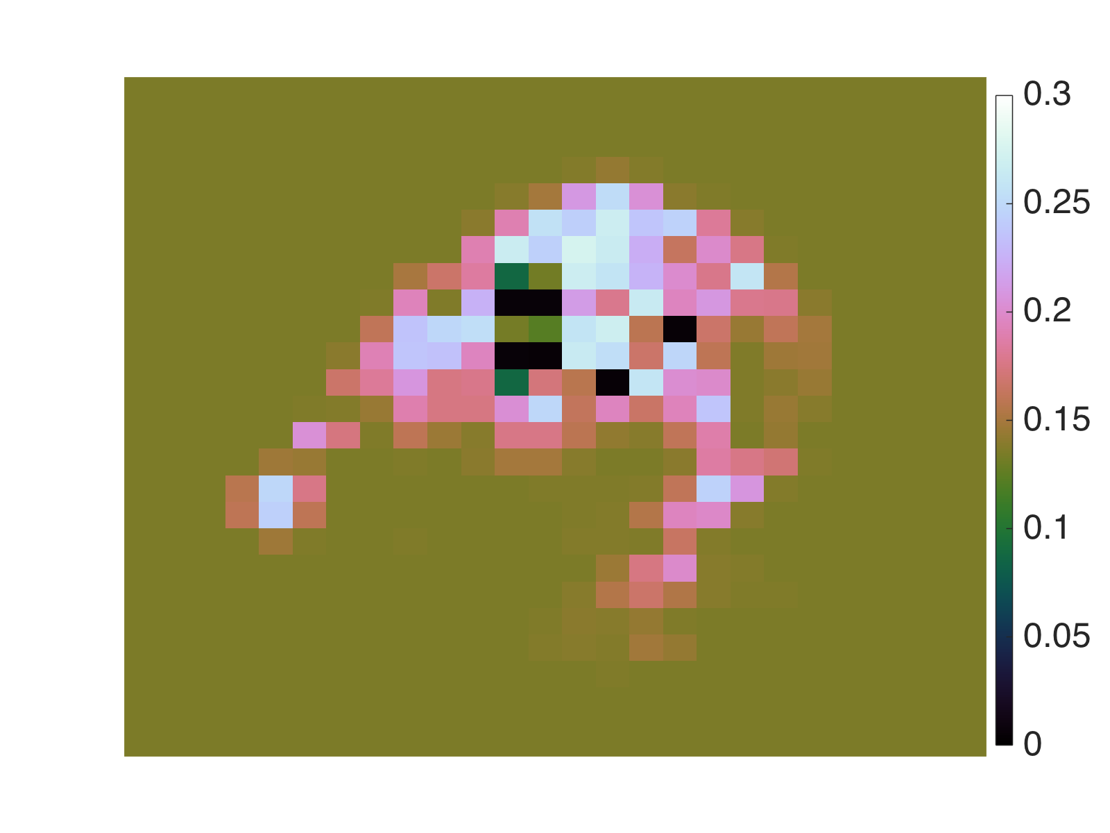
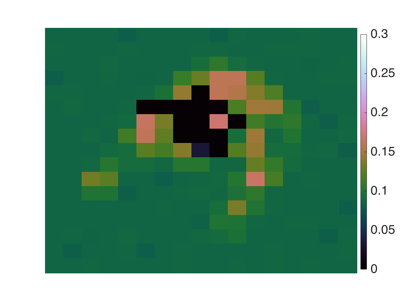
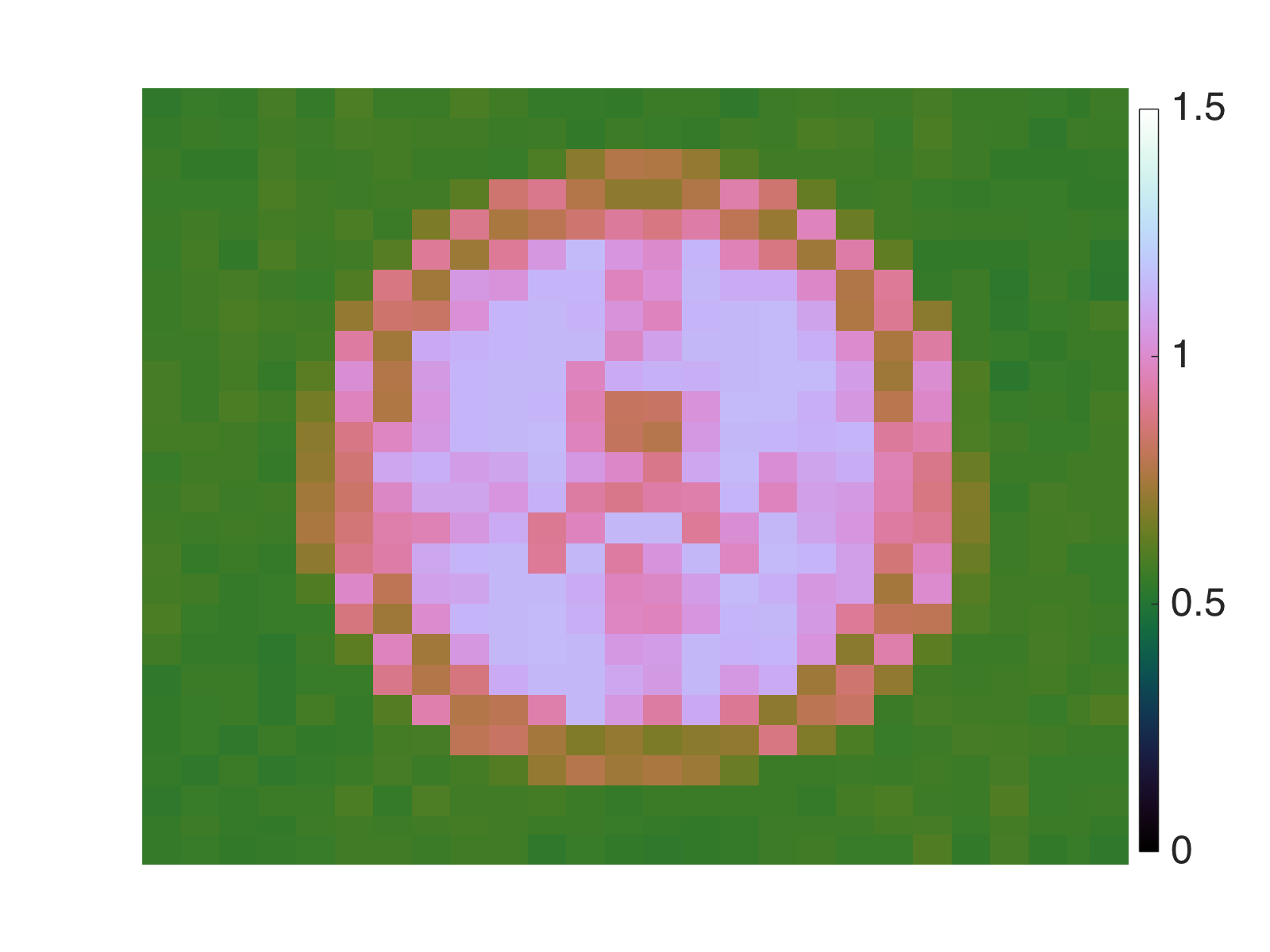
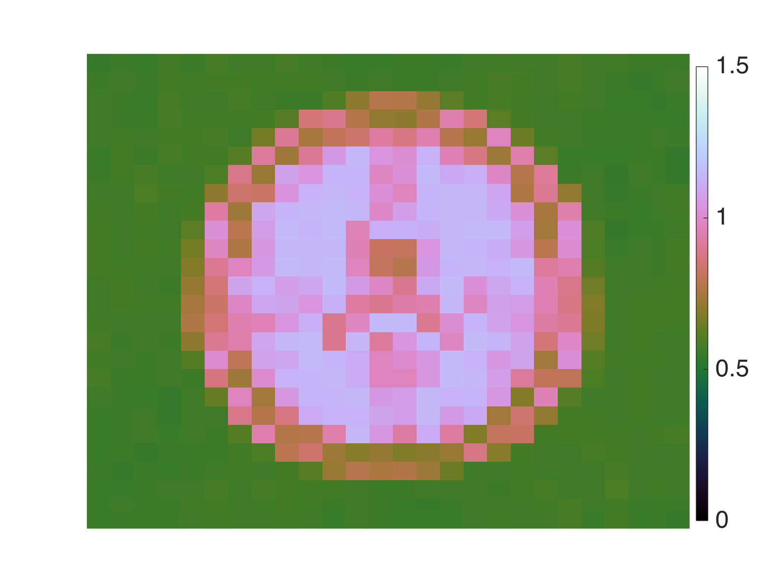
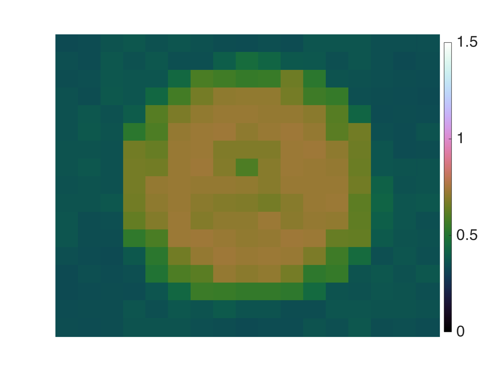
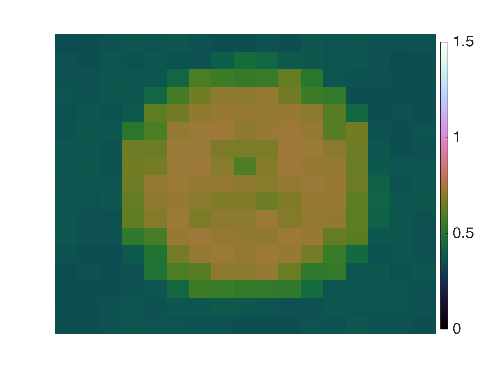
(a) ${\bm{x}}^{*}_{\mu}$	(b) synthesis ($10\times 10$)	(c) analysis ($10\times 10$)	(d) synthesis ($15\times 15$)	(e) analysis ($15\times 15$)

Figure 4: Length of the local credible interval (99% credible level) for RI image M31 (row one) and MRI brain image (row two) (size $256\times 256$). (a) is the computed point estimator for the objective functional equipped with analysis prior and SARA dictionary and is shown in ${\tt log}_{10}$ scale; (b)–(c) and (d)–(e) are the length of the computed local credible interval obtained by equipping SARA dictionary at grid scales of $10\times 10$ and $15\times 15$, respectively.

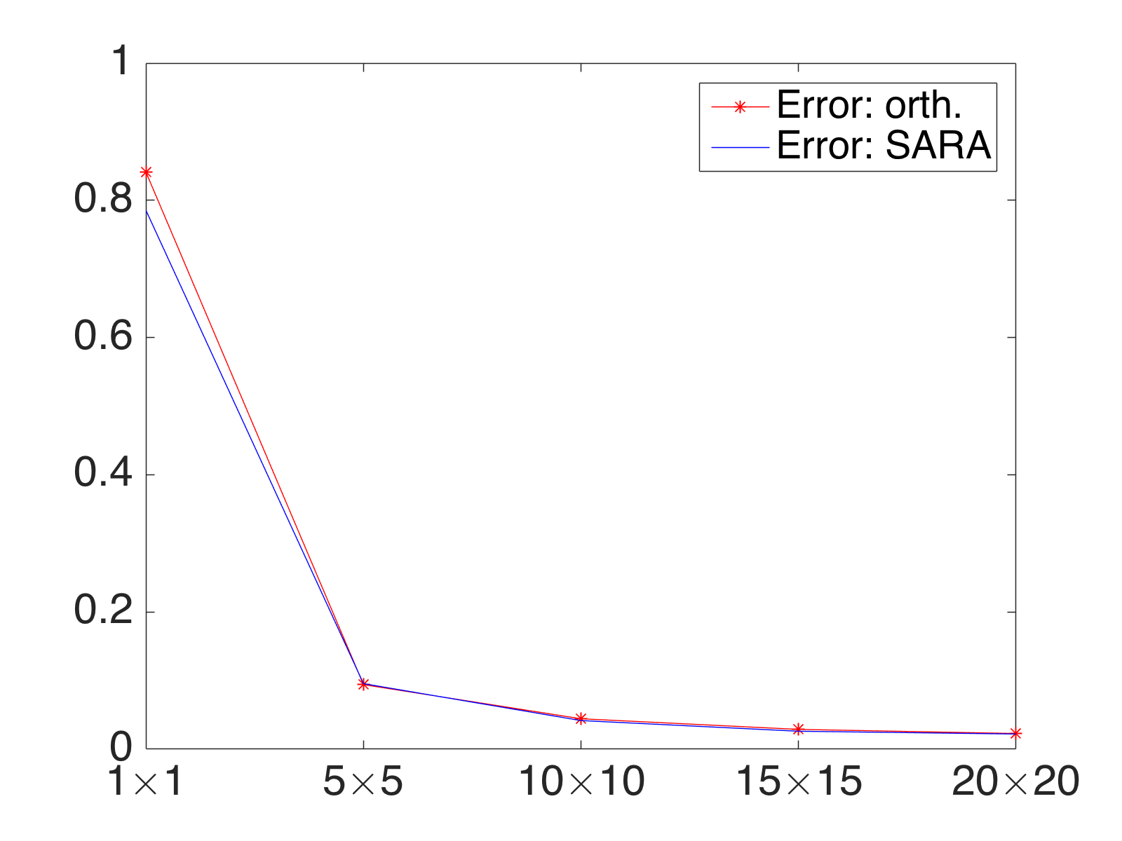
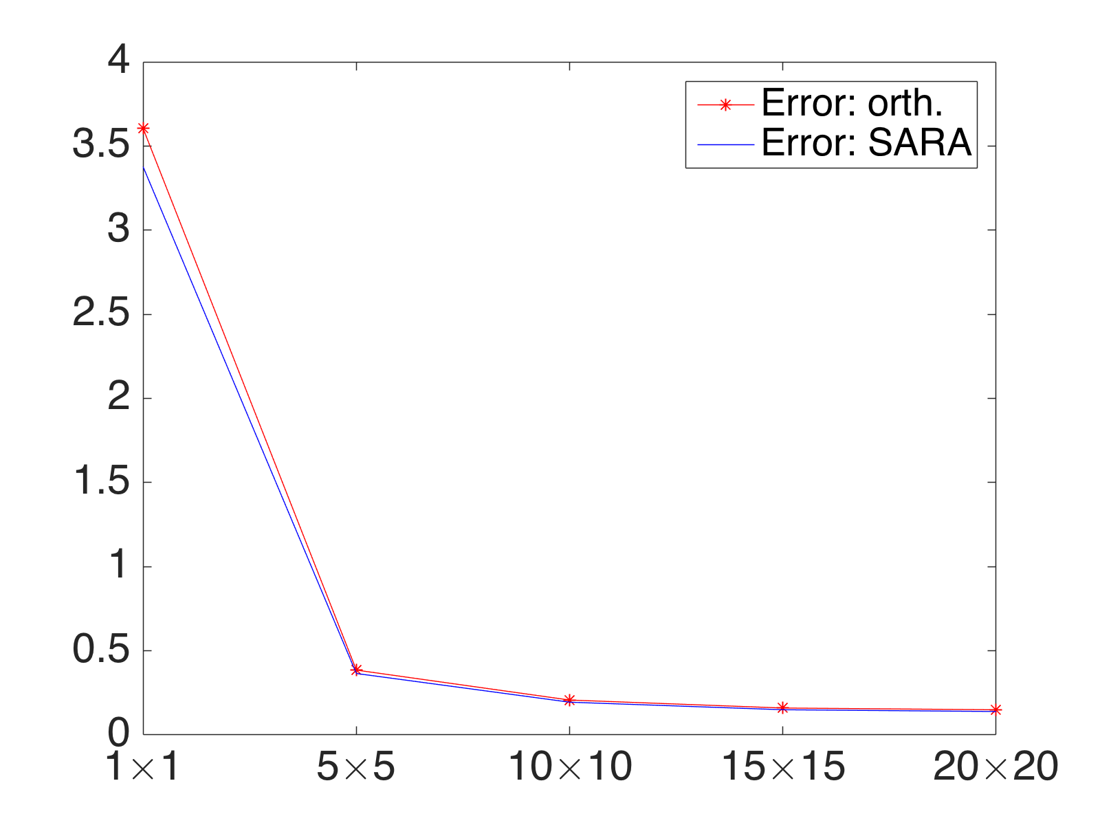
Figure 5: Average relative error (over all pixels) of the length of the local credible interval (99% credible level) computed by MAP estimation, where the dividend of the error is the absolute difference of the length of the local credible interval computed by MAP estimation and Px-MALA, and the divisor is the difference of the maximum and minimum values of the clean image. The analysis prior is used here and the test images are the RI image M31 (left plot) and MRI brain image (right plot). The red line with asterisk and the blue line are the errors regarding the orthonormal basis and SARA dictionary, respectively.

We now illustrate the proposed UQ methodology with a canonical image processing problem – image reconstruction with $\ell_{1}$ prior. The observations (noisy measurement) ${\bm{y}}=\bm{\mathsf{\Phi}}{\bm{x}}+\bm{n}\in\mathbb{C}^{M}$ where $M=N/10$ is used, and $\bm{\mathsf{\Phi}}$ is constructed using Fourier transform followed by a downsampling mask. We consider both the analysis and synthesis priors, i.e., $f(\bm{x})=\|\bm{\mathsf{\Psi}}^{\dagger}{\bm{x}}\|_{1}$ and $f(\bm{a})=\|{\bm{a}}\|_{1}$, respectively. Accordingly, the likelihood functions are set to $g_{\bm{y}}(\bm{x})=\|{\bm{y}}-\bm{\mathsf{\Phi}}{\bm{x}}\|_{2}^{2}/2\sigma^{2}$ and $g_{\bm{y}}(\bm{a})=\|{\bm{y}}-\bm{\mathsf{\Phi}}\bm{\mathsf{\Psi}}{\bm{a}}\|_{2}^{2}/2\sigma^{2}$, where $\sigma=\|\bm{x}^{*}\|_{\infty}10^{{\rm SNR}/20}$ with SNR (signal to noise ratio) set to 30. In contrast to the work in [5, 12], which only used an orthonormal basis for $\bm{\mathsf{\Psi}}$ (Daubechies 8 [DB8]), here we also consider an over-complete basis. Note that an over-complete basis can lead to difference between the analysis and synthesis priors, and therefore is worth investigating. For comparison, we use DB8 wavelets for the orthonormal basis and the over-complete SARA dictionary, consisting of a concatenation of nine bases (DB1–DB8 plus Dirac basis) [13].

The numerical experiments performed in this article were run on a Macbook laptop with an i7 Intel CPU and memory of 16 GB, running MATLAB R2015b. We report experiments with two widely used test data sets – one is M31 (Fig. 2 left) in RI imaging [5, 12] and the other is MRI (magnetic resonance imaging) brain image (Fig. 2 right) in medical imaging [30] – for simulations. Credible regions and intervals are reported at $\alpha=0.01$, i.e., 99% Bayesian confidence. We remark that the test M31 and MRI brain images used here, due to the limited space of the article, are just a showcase of the proposed UQ strategies for general inverse problems. Tests can certainly be performed analogously for other inverse problem applications with different types of images.

The parameter $\mu$ in (3) is estimated via algorithm (4) with 10 iterations and $\gamma,\beta,k=1$. The MAP estimator at each iteration is computed via the forward-backward splitting used in [12]. The automatically estimated parameter $\mu$ associated to the orthonormal basis and SARA dictionary for the analysis prior are reported in Table I, which are then used for the synthesis prior.

Fig. 3 shows the computed threshold $\gamma^{\prime}_{\alpha}$ of the HPD credible regions, which tells us that the difference of the results between synthesis and analysis priors equipped orthonormal basis is negligible, but not for the SARA dictionary. This is consistent with the fact that over-complete basis can lead to a big different between the analysis and synthesis priors for the original inverse problems. Moreover, we found from Table I that the SNR of the point estimators (e.g. see Fig. 4 (a)) using SARA library and the orthonormal basis are different either for the analysis or the synthesis prior, which again shows the difference due to the over-complete basis. Note that the prior with the over-complete SARA dictionary takes greater computation time than that with the orthonormal basis DB8 since SARA contains more sub-bases.

Fig. 4 gives the results of the local credible intervals with respect to grid sizes of $10\times 10$ and $15\times 15$, which shows that all the results are reasonable, and, more importantly, the differences between analysis and synthesis priors and between orthonormal basis and SARA dictionary are subtle (note that the results regarding the orthonormal basis are withdrew here due to the limited space and the negligible different in visual comparison). Fig. 5 shows the error of the length of the local credible interval computed by MAP estimation compared to Px-MALA (a state-of-the-art MCMC method [6]) corresponding to the analysis prior, with both orthonormal basis and SARA dictionary. From Fig. 5, we again see that both bases give very similar local credible interval error, using Px-MALA as the benchmark. Moreover, we see that the error of the MAP estimation is decreasing monotonically regarding different grid scales; particularly, lower than $\sim\!5\%$ when the grid scale is larger than $10\times 10$ (with ${\cal O}(10^{5})$ orders of magnitude faster that Px-MALA).

From the above results we conclude that selecting the regularisation parameter automatically can improve the effectiveness of UQ strategies, applying more complex dictionaries improves the quality of point estimators, and the UQ results are consistent for different prior types and dictionaries. Future works will analyse the sensitivity (or robustness) of the UQ method with respect to the value of the regularisation parameter $\mu$.

V Conclusions

Analysing and quantifying uncertainties for inverse problems in image/signal processing is critical and very challenging since the problems themselves are ill-posed and often high-dimensional. In this article we presented a UQ methodology and investigated a series of UQ strategies based on MAP estimation for general image/signal processing problems. Particularly, in this article, two important new components – automatic regularisation parameter selection and more general dictionaries/bases used in priors – are considered to illustrate and improve the performance of these UQ strategies. Moreover, the experimental results further strengthen the very promising performance of the proposed UQ strategies. We emphasise again that these techniques are based on MAP estimation, and therefore can scale to high-dimensional problems and problems with non-smooth objective functionals (e.g. sparsity-promoting $\ell_{1}$ prior).

References

- [1] L. Pratley, J. D. McEwen, M. d’Avezac, R. E. Carrillo, A. Onose, and Y. Wiaux, “Robust sparse image reconstruction of radio interferometric observations with PURIFY,” MNRAS, vol. 473, pp. 1038–1058, sept 2018.
- [2] J. D. McEwen and Y. Wiaux, “Compressed sensing for wide-field radio interferometric imaging,” MNRAS, vol. 413, pp. 1318–1332, May 2011.
- [3] L. Rudin, S. Osher, and E. Fatemi, “Nonlinear total variation based noise removal algorithms,” Physica D., vol. 60, pp. 259–268, 1992.
- [4] S. Setzer, G. Steidl, and T. Teuber, “Deblurring poissonian images by split bregman techniques,” J. Vis. Commun. Image R., vol. 21, no. 3, pp. 193–199, 2010.
- [5] X. Cai, M. Pereyra, and J. D. McEwen, “Uncertainty quantification for radio interferometric imaging I: proximal-MCMC methods,” MNRAS, vol. 480, pp. 4154–4169, 2018.
- [6] M. Pereyra, “Proximal Markov chain Monte Carlo algorithms,” Statistics and Computing, 2015.
- [7] A. Durmus, E. Moulines, and M. Pereyra, “Efficient Bayesian computation by proximal Markov chain Monte Carlo: when Langevin meets Moreau,” SIAM J. Imaging Sci., vol. 11, pp. 473–506, 2018.
- [8] C. P. Robert, “The Bayesian choice (second edition),” Springer Verlag, New-York, 2001.
- [9] A. Chambolle and T. Pock, “An introduction to continuous optimization for imaging,” Acta Numerica, vol. 25, pp. 161–319, 2016.
- [10] P. L. Combettes and J. C. Pesquet, “Proximal splitting methods in signal processing,” arXiv:0912.3522v4, 2010.
- [11] M. Pereyra, “Maximum a posteriori estimation with Bayesian confidence regions,” SIAM J. Imaging Sci., 2016.
- [12] X. Cai, M. Pereyra, and J. D. McEwen, “Uncertainty quantification for radio interferometric imaging: II. MAP estimation,” MNRAS, vol. 480, pp. 4170–4182, 2018.
- [13] R. E. Carrillo, J. D. McEwen, and Y. Wiaux, “Sparsity Averaging Reweighted Analysis (SARA): a novel algorithm for radio-interferometric imaging,” MNRAS, vol. 426, pp. 1223–1234, Oct. 2012.
- [14] D. L. Donoho, “Compressed sensing,” IEEE Trans. Inf. Theory, vol. 52, pp. 1289–1306, apr 2006.
- [15] R. Tibshirani, “Regression shrinkage and selection via the lasso,” J. Royal. Statist. Soc B., vol. 58, pp. 267–288, 1996.
- [16] X. Cai, R. Chan, and T. Zeng, “A two-stage image segmentation method using a convex variant of the Mumford-Shah model and thresholding,” SIAM J. Imaging Sci., vol. 6, pp. 368–390, 2013.
- [17] M. Pereyra, P. Schniter, E. Chouzenoux, J.-C. Pesquet, J.-Y. Tourneret, A. Hero, and S. McLaughlin, “A survey on stochastic simulation and optimization methods in signal processing,” IEEE Sel. Topics in Signal Processing, vol. 10, pp. 224–241, 2016.
- [18] M. Pereyra, “Revisiting maximum-a-posteriori estimation in log-concave models: from differential geometry to decision theory,” ArXiv e-prints, Dec. 2016.
- [19] P. J. Green, K. Łatuszyński, M. Pereyra, and C. P. Robert, “Bayesian computation: a summary of the current state, and samples backwards and forwards,” Statistics and Computing, vol. 25, no. 4, pp. 835–862, June 2015.
- [20] X. Cai, J. Fitschen, M. Nikolova, G. Steidl, and M. Storath, “Disparity and optical flow partitioning using extended Potts priors,” Information and Inference: A Journal of the IMA, vol. 4, pp. 43–62, 2015.
- [21] S. Boyd, N. Parikh, E. Chu, B. Peleato, and J. Eckstein, “Distributed optimization and statistical learning via the alternating direction method of multipliers,” Foundations and Trends in Machine Learning, vol. 3, no. 1, pp. 1–122, 2010.
- [22] R. E. Carrillo, J. D. McEwen, and Y. Wiaux, “PURIFY: a new approach to radio-interferometric imaging,” MNRAS, vol. 439, pp. 3591–3604, Apr. 2014.
- [23] A. Onose, R. E. Carrillo, A. Repetti, J. D. McEwen, J. P. Thiran, J. C. Pesquet, and Y. Wiaux, “Scalable splitting algorithms for big-data interferometric imaging in the SKA era,” MNRAS, vol. 462, pp. 4314–4335, aug 2016.
- [24] L. Pratley, M. Johnston-Hollitt, and J. D. McEwen, “A fast and exact -stacking and -projection hybrid algorithm for wide-field interferometric imaging,” arXiv:1807.09239, 2018.
- [25] M. Pereyra, J. Bioucas-Dias, and M. Figueiredo, “Maximum-a-posteriori estimation with unknown regularisation parameters,” Signal Processing Conference (EUSIPCO), 2015.
- [26] J. Oliveira, J. Bioucas-Dias, and M. Figueiredo, “Adaptive total variation image deblurring: A majorization-minimization approach,” Signal Process., vol. 89, pp. 1683–1693, 2009.
- [27] J.-C. Pesquet, A. Benazza-Benyahia, and C. Chaux, “A SURE approach for digital signal/image deconvolution problems,” IEEE Trans. Sig. Process., vol. 57, pp. 4616–46 329, 2009.
- [28] C. Deledalle, S. Vaiter, G. Peyre, and J. Fadili, “Stein Unbiased GrAdient estimator of the Risk (SUGAR) for multiple parameter selection,” SIAM J. Imaging Sci., vol. 7, pp. 2448–2487, 2014.
- [29] R. E. Carrillo, J. D. McEwen, D. V. D. Ville, J.-P. Thiran, and Y. Wiaux, “Sparsity averaging for compressive imaging,” IEEE Sig. Proc. Let., vol. 20, no. 6, pp. 591–594, 2013.
- [30] Brainweb: Simulated brain database. [Online]. Available: http://brainweb.bic.mni.mcgill.ca/brainweb/