Optical Wireless Cochlear Implants

Abstract

In the present contribution, we introduce a wireless optical communication-based system architecture which is shown to significantly improve the reliability and the spectral and power efficiency of the transcutaneous link in cochlear implants (CIs). We refer to the proposed system as optical wireless cochlear implant (OWCI). In order to provide a quantified understanding of its design parameters, we establish a theoretical framework that takes into account the channel particularities, the integration area of the internal unit, the transceivers misalignment, and the characteristics of the optical units. To this end, we derive explicit expressions for the corresponding average signal-to-noise-ratio, outage probability, ergodic spectral efficiency and capacity of the transcutaneous optical link (TOL). These expressions are subsequently used to assess the dependence of the TOL’s communication quality on the transceivers design parameters and the corresponding channels characteristics. The offered analytic results are corroborated with respective results from Monte Carlo simulations. Our findings reveal that OWCI is a particularly promising architecture that drastically increases the reliability and effectiveness of the CI TOL, whilst it requires considerably lower transmit power compared to the corresponding widely-used radio frequency (RF) solution.

1 Introduction

During the past decades, medical implants have been advocated as an effective solution to numerous health issues due to the quality of life improvements they can provide. One of the most successful application of such devices is cochlear implants (CIs), which have restored partial hearing to more than $350,000$ people worldwide, half of whom are pediatric users who ultimately develop nearly normal language capability [1, 2]. A typical CI consists of an out-of-body unit, which uses a microphone to capture the sound, converts it into a radio frequency (RF) signal and wirelessly transmits it to an in-body unit. Conventional CIs exploit near-field magnetic communication technologies and typically operate in low RF frequencies, from $5$ MHz to $49$ MHz, while their transmit power is in the order of tens of $\mathrm{mW}$ [2, 3, 4, 5]. However, the main disadvantage of this technology is that it cannot support high data rates which are required for neural prosthesis applications in order to achieve similar performance to that of human organs, such as the cochlea, under reasonable transmit power constraints [6, 7, 8]. By also taking into account the interference from other sources operating in the same frequency band, RF transmission is largely rendered a mediocre solution [9, 10, 11].

Overcoming the above constraints in CIs calls for investigations on the feasibility of transcutaneous wireless links that operate in non-standardized frequency bands. In light of this and due to the increased bandwidth availability, the partial transparency of skin at infrared wavelengths and the remarkably high immunity to external interference, the use of optical wireless communications (OWCs) has been recently introduced as an attractive alternative solution to the conventional approach (see [12, 13, 14] and the references therein). The feasibility of OWCs for the transcutaneous optical link (TOL) has been experimentally validated in numerous contributions [15, 16, 17, 18, 10, 19, 20, 21, 22]. Specifically, TOLs were used in [15] to establish transdermal high data rate communications between the internal and external units of a medical system. Additionally, the TOL’s primary design parameters and their interaction were quantified in [16], whilst the authors in [17] reported the tradeoffs related to the design of OWC based CI. In the same context, the authors in [19] evaluated the performance of a TOL utilized for clinical neural recording purposes in terms of tissue thickness, data rate and transmit power. Furthermore, the characteristics of the receiver were investigated with regard to its size and the signal-to-noise-ratio (SNR) maximization. In [10], a low power high data rate optical wireless link for implantable transmission was presented and evaluated in terms of power consumption and bit-error-rate (BER), for a predetermined misalignment tolerance. Likewise, the authors in [20] verified in-vivo the feasibility of TOL, proving that high data rates - even in the order of $100$ Mbps - can be delivered with a BER of $2\times 10^{-7}$ in the presence of misalignment fading. Nevertheless, these high data rates have been achieved at the cost of high power consumption [23], which reached $2.1\text{ }mW$. In contrast to [20], the authors in [18] presented novel experimental results of direct and retroreflection transcutaneous link configurations and their findings verified the feasibility of highly effective and robust low-power consumption TOLs. Finally, a bidirectional transcutaneous optical telemetric data link was reported in [21], whereas a bidirectional transcutaneous optical data transmission system for artificial hearts, allowing long-distance data communication with low electric power consumption, was described in [22].

Table 1: Comparison between OWCIs and RFCIs.

OWCIs	RFCIs
Unprecedented increase	Relatively limited
in bandwidth	bandwidth
High achievable data rate	Mediocre data rate
Low interference: Solar and
ambient light are the main sources	Very high interference from other
of interference and can be	electronic and electrical appliances
easily mitigated or even cancelled
Safer for the human health	Of questionable safety
due to the low transmission power	concerning the human body
Low power demands	High power demands
Comparable cost
Mature technology that can exploit
the particularities of novel materials	Mature technology
(e.g. graphene) to achieve improved	that allows compact designs
features in the same integration area
Existing design guidelines from several	Matured
standards (i.e. IEEE Std 1073.3.2-2000,	standardization
IEC Laser Safety Standard, IrDA,	(i.e. IEEE 802.15.4,
JEITA​ Cp-1223,​ European​ COST 1101,​ etc.)	IEEE Std 1073.3.2-2000, etc.)
Stringent alignment requirements	Susceptible misalignment

To the best of the authors’ knowledge, the use of OWCs for establishing TOLs in CIs has not been reported in the open technical literature. Motivated by this, in the present work, we propose a novel system architecture which by employing OWCs improves the reliability as well as the spectral and power efficiency of the TOL. We refer to this architecture as optical wireless cochlear implant (OWCI). A list of the advantages and disadvantages of the OWCI and RF cochlear implant (RFCI) is depicted in Table 1. It is noted that OWCI is in line with the advances in CIs, since the use of optics for the stimulation of the acoustic nerve has been recently proposed [7, 24, 25, 26, 27, 28]. In addition, we evaluate the feasibility and the capabilities of the proposed system whilst we provide design guidelines for the OWCI. Specifically, the technical contribution of this paper is summarized below:

• We establish an appropriate system model for the TOL, which includes all different design parameters and their corresponding interactions. These parameters include the thickness of the skin through which the light is transmitted, the size of the integration area of the optics, the degree of transmitter (TX) and receiver (RX) misalignment, the efficiency of the optical system, and the emitter power.

• We derive a comprehensive analytical framework that quantifies and evaluates the feasibility and effectiveness of the OWC link in the presence of misalignment fading. In this context, we provide novel closed-form expressions for the instantaneous and average SNR, which quantifies the received signal quality. Additionally, we evaluate the outage performance and the capacity of the optical link by deriving tractable analytic expressions for the outage probability and the spectral efficiency. These expressions take into account the technical characteristics of the link as well as the transcutaneous medium particularities; hence, they provide meaningful insights into the behavior of the considered set up, which can be used as design guidelines of such systems. Finally, we deduce novel expressions and simple bounds/approximations for the evaluation of the OWCI capacity. Interestingly, our findings reveal the superior reliability and effectiveness of OWCI compared to the baseline CI RF solution.

The remainder of this paper is organized as follows: The system model of the OWCI is described in Section 2. In Section 3, we provide the analytical framework for quantifying the performance of the OWCI by deriving novel analytic expressions for the instantaneous and average SNR, the outage probability, as well as the spectral efficiency and the channel capacity. Respective numerical and simulation results, which illustrate the performance of the OWCI along with useful related discussions are provided in Section 4. Finally, closing remarks and a summary of the main findings of this contribution are presented in Section 5.

Notations: Unless stated otherwise, in this paper, $|\cdot|$ denotes absolute value, $\exp(\cdot)$ represents the exponential function, while $\log_{2}(\cdot)$ and $\ln(\cdot)$ stand for the binary logarithm and the natural logarithm, respectively. In addition, $P\left(\mathcal{A}\right)$ denotes the probability of the event $\mathcal{A}$, whereas $\mathrm{erf}(\cdot)$ denotes the error function and $\Phi(\cdot,\cdot,\cdot)$ represents the Lerch $\Phi$ function [29].

2 System model

As illustrated in Fig. 1, the main parts of the OWCI are the external unit, the propagation medium (skin) and the internal unit [30, 31]. The external unit consists of a microphone that captures the sound, followed by the sound processor responsible for the digitization and compression of the captured sound into coded signals. The coded signal is then forwarded to the transmitter (TX), which conveys the data to the RX in the internal unit. The internal unit consists of the RX which is embedded in the skull, a digital signal processing (DSP) unit, a stimulation (STM) unit and an electrode array implanted in the cochlea. The DSP and STM units operate together in order to modulate the received signal into pulses of electrical current that are capable of stimulating the auditory nerve. Finally, the electrode array delivers the signal to the auditory nerve, where it is interpreted as sound by the brain.

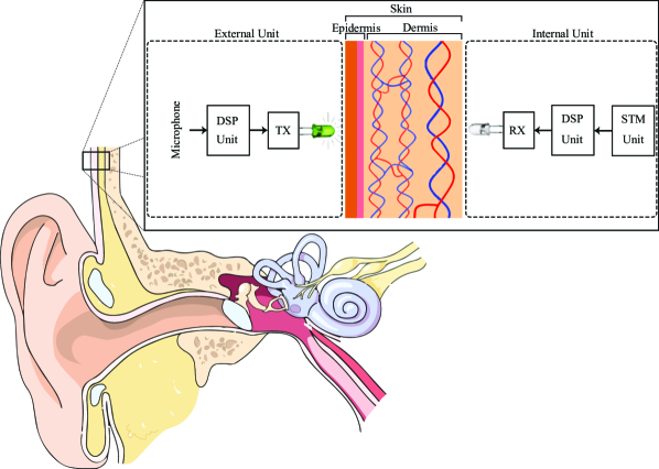
Figure 1: System architecture of OWCI. In this figure ‘DSP unit’ and ‘STM unit’ denote the digital signal processing and stimulation units, respectively.

We assume that the transmitted signal, $x$, is conveyed over the wireless channel, $h$, with additive noise $n$. Therefore, the baseband equivalent received signal can be expressed as [32, 33, 34]

$$y=Rhx+n$$ (1)

where $R$ denotes the responsivity of the RX’s photodiode, which is given by

$$R=\eta\frac{q}{pv}.$$ (2)

In (2), $\eta$ represents the quantum efficiency of the photodiode, $q$ is the electron charge, $v$ denotes the photons’ frequency and $p$ is the Planck’s constant.

Likewise, the channel, $h$, can be expressed as [18]

$$h=h_{l}h_{p}$$ (3)

where $h_{l}$ and $h_{p}$ denote, respectively, the deterministic channel coefficient, due to the propagation loss, and the stochastic process that models the geometric spread, due to the misalignment fading. Also, we assume a Gaussian spatial intensity profile of the beam waste on the RX plane at distance $\delta$ from the TX, $w_{\rm\delta}$, and a circular aperture of radius $\beta$. As a result, the stochastic term of the channel coefficient, $h_{p}$, represents the fraction of the collected power due to geometric spread with radial displacement $r$ from the origin of the detector. Moreover, by assuming that the elevation and the horizontal displacement (sway) follow independent and identical Gaussian distributions, as in [35], we observe that the radial displacement at the RX follows a Rayleigh distribution.

To this effect, the deterministic term of the channel coefficient can be evaluated as [36, eq. 10.1]

$$h_{l}=\exp\left(-\frac{1}{2}\alpha(\lambda)\delta\right)$$ (4)

where $\alpha(\lambda)$ represents the skin attenuation coefficient at wavelength $\lambda$ and $\delta$ denotes the total dermis thickness, which is approximately equivalent to the TX-RX distance. The skin attenuation coefficient can be derived from [37, 38, 39, 40, 41, 42, 43]. It is worth noting that according to [36], the term skin refers to the complex biological structure composed by three essential layers, namely stratum corneum, epidermis, and dermis. Furthermore, as in [10], the TX and the RX are in contact with the outer (epidermal) and inner (adipose) side of the skin. As a result, the distance between TX and RX can be approximated by the skin thickness.

In the same context, the noise component can be expressed as

$$n=n_{\rm s}+n_{\rm th}$$ (5)

where $n_{\rm s}$, and $n_{\rm th}$ represent the shot noise and the thermal noise, respectively, which can be modelled as zero-mean Gaussian processes [13].

In more detail, the shot noise can be expressed as

$$n_{\rm s}=n_{b}+n_{\rm DC}$$ (6)

where $n_{b}$, and $n_{\rm DC}$ represent the background shot noise and dark current shot noise, respectively, which can be also modeled as a zero-mean Gaussian processes with variances

$$\sigma_{b}^{2}=2qRBP_{b}$$ (7)

and

$$\sigma_{\rm DC}^{2}=2qBI_{\rm DC}$$ (8)

respectively [18, 34]. It is noted that the term $B$ in (7) and (8), denotes the communication bandwidth, $R$ is the responsivity of the detector, $P_{b}$ is the background optical power, and $I_{\rm DC}$ is the intensity of the dark current which is generated by the photodetector in the absence of background light, and stems from thermally generated electron–hole pairs.

Finally, $n_{\rm th}$ represents the thermal noise, which is caused by thermal fluctuations of the electric carriers in the receiver circuit, and can be modelled as a zero-mean Gaussian process with variance $\sigma_{\rm th}^{2}$. As a result, since $n_{b}$, $n_{\rm DC}$, and $n_{\rm th}$ are zero-mean Gaussian processes [18, 13], $n$ also follows a zero-mean Gaussian distribution with variance

$$\sigma^{2}=\sigma_{\rm b}^{2}+\sigma_{\rm DC}^{2}+\sigma_{\rm th}^{2}.$$ (9)

3 Performance analysis

In this section, we provide the mathematical framework that quantifies the performance of the proposed system. In this context, we derive closed-form expressions for the instantaneous and average SNR, outage probability and ergodic spectral efficiency and capacity. Capitalizing on them, we also derive simple and tight lower bounds for the ergodic capacity that provide useful insights. Hence, these expressions can be used to validate the feasibility of the system as well as to introduce design guidelines for its effective utilization.

3.1 Evaluation of the average SNR

Based on (1)-(9), the instantaneous SNR can be obtained as [44]

$$\gamma=\frac{R^{2}\exp\left(-\alpha(\lambda)\delta\right)h_{p}^{2}P_{s}}{2qRBP_{b}+2qBI_{\rm DC}+\sigma_{\rm th}^{2}}$$ (10)

or equivalently

$$\gamma=\frac{R^{2}\exp\left(-\alpha(\lambda)\delta\right)h_{p}^{2}\tilde{P}_{s}}{2qRP_{b}+2qI_{\rm DC}+N_{0}}$$ (11)

where $P_{s}$ denotes the average optical power of the transmitted signal, whereas $\tilde{P}_{s}$ and $N_{0}$ represent the signal and noise optical power spectral density (PSD), respectively.

The average SNR in the considered set up is derived in the following theorem.

Theorem 1

The average SNR in the considered system can be expressed as

$$\tilde{\gamma}=\frac{R^{2}\exp\left(-\alpha(\lambda)\delta\right)\tilde{P}_{s}}{2qRP_{b}+2qI_{\rm DC}+N_{0}}\frac{\xi A_{0}^{2}}{\xi+2}$$ (12)

where  [45]

$$A_{0} =[\operatorname{erf}\left(\upsilon\right)]^{2}$$ (13)

denotes the fraction of the collected power in case of zero radial displacement, with

$$\upsilon=\frac{\sqrt{\pi}\beta}{\sqrt{2}w_{\rm\delta}}.$$ (14)

In the above equations, $\beta$ and $w_{\rm\delta}$ denote, respectively, the radius of the RX’s circular aperture and the beam waste (radius calculated at $e^{-2}$) on the RX plane at distance $\delta$ from the TX. Moreover, $\xi$ is the square ratio of the equivalent beam radius, $w_{\rm eq}$, and the pointing error displacement standard deviation at the RX, namely

$$\xi=\frac{w_{\rm eq}^{2}}{4\sigma_{s}^{2}}$$ (15)

with $\sigma_{s}^{2}$ denoting the pointing error displacement (jitter) variance at the RX, whereas

$$w_{\rm eq}^{2} =w_{\rm\delta}^{2}\frac{\sqrt{\pi}\operatorname{erf}\left(\upsilon\right)}{2\upsilon\exp\left(-\upsilon^{2}\right)}.$$ (16)

Proof 1

The proof is provided in Appendix A.

From (12), it is evident that the average SNR depends on the transmission PSD, the skin particularities, namely skin attenuation and thickness, the RX’s characteristics, and the intensity of the misalignment fading. It is also noted that since the skin attenuation is a function of the wavelength, the average SNR is also a function of the wavelength.

3.2 Evaluation of the ergodic spectral efficiency

In this section, we quantify the OWCI capability in terms of spectral efficiency. In this context, a novel closed-form expression for the ergodic spectral efficiency of the proposed system is derived in the following theorem.

Theorem 2

The ergodic spectral efficiency of the considered set up can be expressed as

$$C=\frac{1}{2}\log_{2}\left(1+\mathcal{B}(\lambda)A_{0}^{2}\right)-\frac{1}{2}\frac{A_{0}^{2}\mathcal{B}(\lambda)}{\ln(2)}\Phi\left(-A_{0}^{2}\mathcal{B}(\lambda),1,1+\frac{\xi}{2}\right)$$ (17)

where

$$\mathcal{B}(\lambda)=\frac{\psi R^{2}\exp\left(-\alpha(\lambda)\delta\right)\tilde{P}_{s}}{2qRP_{b}+2qI_{\rm DC}+N_{0}}.$$ (18)

Proof 2

The proof is provided in Appendix B.

It is recalled that the Shannon ergodic spectral efficiency in $C=\tfrac{1}{2}\mathbb{E}\left[\log_{2}\left(1+\psi\gamma\right)\right]$ is a valid exact expression for deriving the ergodic spectral efficiency for the heterodyne detection technique, while it acts as a lower bound for the IM/DD scheme [46, eq. (26)] and [47, eq. (7.43)]. Hence, the derived ergodic spectral efficiency in (17) is correspondingly an exact solution for the heterodyne detection technique and a lower bound for the IM/DD technique.

Furthermore, it is noticed that (17) is an exact closed-form expression that can be straightforwardly computed using popular software packages. Based on this, we can also derive a simple lower bound for the ergodic spectral efficiency that provide useful insights on the impact of the involved parameters.

Proposition 1

The ergodic spectral efficiency can be lower bounded as follows:

$$C>\frac{1}{2}\log_{2}\left(1+\mathcal{B}(\lambda)A_{0}^{2}\right)-\frac{1}{\xi\ln(2)}$$ (19)

Proof 3

The proof is provided in Appendix C.

It is noted here that the above lower bound is particularly tight; as a result, equation (19) can also considered as a highly accurate bounded approximation of the ergodic spectral efficiency.

Based on the above and with the aid of (12), it follows that (17) can be equivalently rewritten as

$$C=\frac{1}{2}\log_{2}\left(1+\psi\frac{\xi+2}{\xi}\tilde{\gamma}\right)-\frac{\psi}{2\ln(2)}\frac{{\xi+2}}{{\xi}}\tilde{\gamma}\Phi\left(-\psi\frac{\xi+2}{\xi}\tilde{\gamma},1,1+\frac{\xi}{2}\right)$$ (20)

which with the aid of Proposition 1 it can be lower bounded as follows:

$$C=\frac{1}{2}\log_{2}\left(1+\psi\frac{\xi+2}{\xi}\tilde{\gamma}\right)-\frac{1}{\xi\ln(2)}.$$ (21)

It is noticed in (20) that the ergodic spectral efficiency depends on the level of misalignment, modeled by the term $\xi$, and the average SNR.

3.3 Evaluation of the ergodic capacity

Based on the presented channel model, the optical transcutaneous link is wavelength selective. Also, the bandwidth over which the channel transfer function remains virtually constant is hereby denoted as $\Delta f$. Thus, the capacity can be obtained by dividing the total bandwidth, $B$, into $K$ narrow sub-bands and then summing up the individual capacities [48]. The $i^{th}$ sub-band is centered around the wavelength $\lambda_{i}$, with $i\in[1,K]$, and it has width $\Delta f$. If the subband width is sufficiently small, the sub-channel appears as wavelength non-selective. As a consequence, by assuming full CSI knowledge at both the TX and the RX, the resulting capacity in $\mathrm{bits/s}$ can be expressed as

$$C_{\rm B}=\frac{1}{2}\sum_{\rm i=1}^{K}\Delta f\left(\log_{2}\left(1+\mathcal{B}(\lambda_{i})A_{0}^{2}\right)-\frac{A_{0}^{2}\mathcal{B}(\lambda_{i})}{\ln(2)}\Phi\left(-A_{0}^{2}\mathcal{B}(\lambda_{i}),1,1+\frac{\xi}{2}\right)\right).$$ (22)

Of note, for the special case in which $B\leq\Delta f$, equation (22) becomes

$$C_{B}=\frac{1}{2}B\log_{2}\left(1+\mathcal{B(\lambda)}A_{0}^{2}\right)-\frac{1}{2}B\frac{A_{0}^{2}\mathcal{B(\lambda)}}{\ln(2)}\Phi\left(-A_{0}^{2}\mathcal{B(\lambda)},1,1+\frac{\xi}{2}\right)$$ (23)

which is a common case since the values of $\Delta f$ are in the order of $\mathrm{GHz}$, whereas those of $B$ are in the order of $\mathrm{MHz}$. Based on this and with the aid of Proposition 1, equations (22) and (23) can be lower bounded as follows:

$$C_{\rm B}>\frac{1}{2}\sum_{\rm i=1}^{K}\Delta f\log_{2}\left(1+\mathcal{B}(\lambda_{i})A_{0}^{2}\right)-\frac{1}{\xi\ln(2)}$$ (24)

and

$$C_{B}>\frac{1}{2}B\log_{2}\left(1+\mathcal{B(\lambda)}A_{0}^{2}\right)-\frac{B}{\xi\ln(2)}$$ (25)

respectively. As in the previous scenarios, the above inequalities are particularly tight; as a result, they can be also considered as simple and accurate approximations.

3.4 Evaluation of the outage probability

The reliability of the OWCI can be additionally evaluated in terms of the corresponding outage performance. To this end, we derive the outage probability of the considered set up in the presence of misalignment fading which is a critical factor in optical wireless communication systems.

Theorem 3

The outage probability of the considered system can be expressed as

$$P_{o}(\gamma_{\rm th})=\left\{\begin{array}[]{c c}\frac{1}{A_{0}^{\xi}}\left(\frac{2qRP_{b}+2qI_{\rm DC}+N_{0}}{R^{2}\exp\left(-\alpha(\lambda)\delta\right)\tilde{P}_{s}}\gamma_{\rm th}\right)^{\tfrac{\xi}{2}},&\gamma_{\rm th}\leq\frac{R^{2}\exp\left(-\alpha(\lambda)\delta\right)A_{0}^{2}\tilde{P}_{s}}{2qRP_{b}+2qI_{\rm DC}+N_{0}},\\ 1,&\text{ otherwise. }\end{array}\right.$$ (28)

Proof 4

The proof is provided in Appendix D.

From (28), it is evident that the maximum spectral efficiency is constrained by the PSD of the noise components, the RX’s responsivity, the pathloss, and the intensity of the misalignment effect. Furthermore, we observe that as the transmission signal PSD increases, the spectral efficiency constraint relaxes.

According to (12) and (28), the outage probability can be alternatively expressed as

$$P_{o}(r_{\rm th})=\left\{\begin{array}[]{c c}\left(\frac{\xi}{\xi+2}\frac{\gamma_{\rm th}}{\tilde{\gamma}}\right)^{\frac{\xi}{2}},&\gamma_{\rm th}\leq\frac{\xi+2}{\xi}\tilde{\gamma},\\ 1,&\text{ otherwise }\end{array}\right.$$ (31)

which indicates that for given $\gamma_{\rm th}$ and $\tilde{\gamma}$, the outage performance of OWCI improves as $A_{0}$ increases. Moreover, it is shown that for a fixed $\gamma_{\rm th}$ and $A_{0}$, the outage probability decreases as $\tilde{\gamma}$ increases. Finally, it is observed that as $\gamma_{\rm th}$ increases, the outage probability also increases.

3.5 Pointing error displacement tolerance in practical OCWI designs

It is evident that the derived analytic expressions in the previous sections allow the determination of the pointing error displacement (jitter) and its variance for given quality of service requirements. To this end, it readily follows from (28) that

$$\begin{array}[]{c c}\sigma_{s}^{2}=\frac{w_{\rm eq}^{2}}{8\log_{\mathcal{H}}(P_{o}(\gamma_{\rm th}))}=\frac{w_{\rm eq}^{2}\ln(\mathcal{H})}{8\ln(P_{o}(\gamma_{\rm th}))},&\qquad\gamma_{\rm th}\leq\frac{R^{2}\exp\left(-\alpha(\lambda)\delta\right)A_{0}^{2}\tilde{P}_{s}}{2qRP_{b}+2qI_{\rm DC}+N_{0}}\end{array}$$ (32)

and

$$\begin{array}[]{c c}\sigma_{s}=\frac{w_{\rm eq}\sqrt{\ln(\mathcal{H})}}{2\sqrt{2\ln(P_{o}(\gamma_{\rm th}))}}=\frac{w_{\rm eq}}{2\sqrt{2}}\sqrt{\frac{\alpha(\lambda)\delta+\ln(\gamma_{\rm th})+\ln(2qRP_{b}+2qI_{\rm DC}+N_{0})-2\ln(A_{0})-2\ln(R)-\ln(\tilde{P}_{s})}{\ln(P_{o}(\gamma_{\rm th}))}}\end{array}$$ (33)

where

$$\mathcal{H}=\frac{2qRP_{b}+2qI_{\rm DC}+N_{0}}{A_{0}^{2}R^{2}\exp\left(-\alpha(\lambda)\delta\right)\tilde{P}_{s}}\gamma_{\rm th}.$$ (34)

The above expressions provide useful insights into the practical design of OCWI, since they allow the quantification of the amount of pointing error displacement, and its variance, that can be tolerated with respect to certain outage probability requirements. More specifically, the system parameters, in the practical designs, will be initially selected in order to achieve a target outage probability that is slightly better than the target one, under the assumption of no pointing error displacement. Then, using (33) and setting in it the exact target outage probability will determine the amount of pointing error displacement that can be tolerated for this particular system and quality of service requirements. Conversely, for pointing error displacement levels that constrain the target quality of service requirements, these equations can assist in determining the required countermeasures for the incurred detrimental effects.

Finally, the above expressions allow us to express the ergodic capacity representation in (23) in terms of the corresponding outage probability, namely

$$C_{B}=\frac{B}{2}\log_{2}\left(1+\mathcal{B(\lambda)}A_{0}^{2}\right)-\frac{BA_{0}^{2}\mathcal{B(\lambda)}}{2\ln(2)}\Phi\left(-A_{0}^{2}\mathcal{B(\lambda)},1,1+\frac{\ln(P_{o}(\gamma_{\rm th}))}{\ln(\mathcal{H})}\right)$$ (35)

which in turn allows the quantification of the required ergodic capacity for certain design parameters and target outage probability requirements. In addition, further insights on the role of the involved parameters on the overall system performance can be obtained by tightly lower bounding (35) with the aid of Proposition 1, namely

$$C_{B}>\frac{B}{2}\log_{2}\left(1+\mathcal{B(\lambda)}A_{0}^{2}\right)-\frac{B\ln(\mathcal{H})}{2\ln(2)\ln(P_{o}(\gamma_{\rm th})}.$$ (36)

It is noted that similar expressions can be deduced if (28) is solved with respect to other involved design parameters.

4 Numerical results & discussion

In this section, we evaluate the feasibility and effectiveness of OWCI by providing analytical results and insights for different scenarios of interest as well as sets of design parameters. The validity of the offered analytical results is extensively verified by respective results from Monte Carlo simulations. Unless otherwise stated, we henceforth assume that the photodiode (PD) effective area, $A=\pi\beta^{2}$, with $\beta$ denoting the radius of the RX’s circular aperture, is $1\text{ }\mathrm{mm}^{2}$. Also, we assume that the divergence angle, $\theta$, is $20^{o}$, whilst the skin thickness, $\delta$, is assumed to be equal to $4\text{ }\mathrm{mm}$ and the noise optical PSD, $N_{\rm 0}$, is set to $\left(1.3\text{ }\mathrm{pA/\sqrt{Hz}}\right)^{2}$ [49]. The beam waist at distance $\delta$ is determined  by $w_{\rm\delta}=\delta\tan\left(\theta/2\right)$, and the pointing error displacement variance, $\sigma_{\rm s}$, is assumed to be $0.5\text{ }\mathrm{mm}$. Moreover, according to [18] the TOL exhibits remarkably high immunity to external interference. In addition, in the following analysis we ignore the noise from external light sources by considering a dark-shielded receiver-to-skin interface. As a result, the background optical power can be omitted, i.e., $P_{\rm b}=0$. Furthermore, the PD’s dark current, $I_{\rm DC}$, is set to $0.05\text{ }\mathrm{nA}$ whereas the quantum efficiency of the PD, $\eta$, is $0.8$ [36]. Finally, the transmitted signal power, $P_{\rm s}$, and PSD, $\tilde{P}_{\rm s}$, are $0.1\text{ }\mathrm{\mu W}$ and $0.01\text{ }\mathrm{\mu W/MHz}$, respectively, the communication bandwidth, $B$, is $10\text{ }\mathrm{MHz}$, the data rate threshold, $r_{\rm th}$, is set to $=1\text{ }\mathrm{bits/s/Hz}$, the operation wavelength, $\lambda$, is $=1100\text{ }\mathrm{nm}$ and the square ratio between the equivalent beam radius and the pointing error displacement standard deviation (SD) at the RX, $\xi$, is assumed to be $1$.

The remainder of this section is organized as follows: The impact of the skin thickness on the performance of the OWCI is described in Section 4.1, while the degradation of the TOL due to the misalignment fading is presented in Section 4.2. The joint effect of the skin thickness and the misalignment is provided in Section 4.3. Finally, the impact of various design parameters is analyzed in Section 4.4.

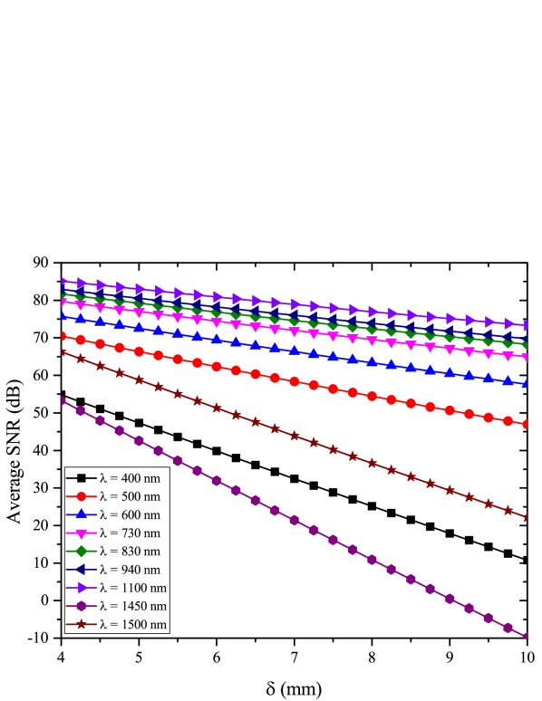
(a) Average SNR vs skin thickness for different values of wavelength.

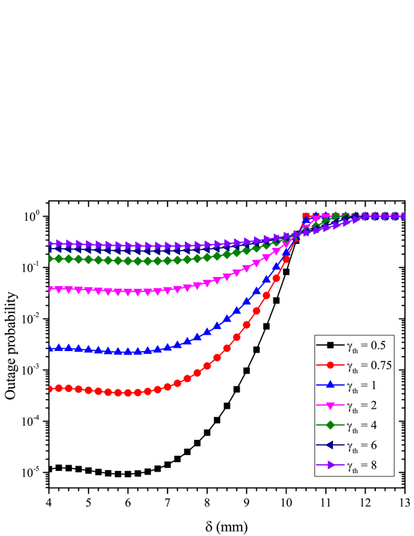
(b) Outage probability vs skin thickness for different values of SNR threshold, for $\lambda=1500\text{ }\mathrm{nm}$.

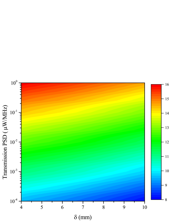
(c) Spectral efficiency vs skin thickness and transmission PSD.

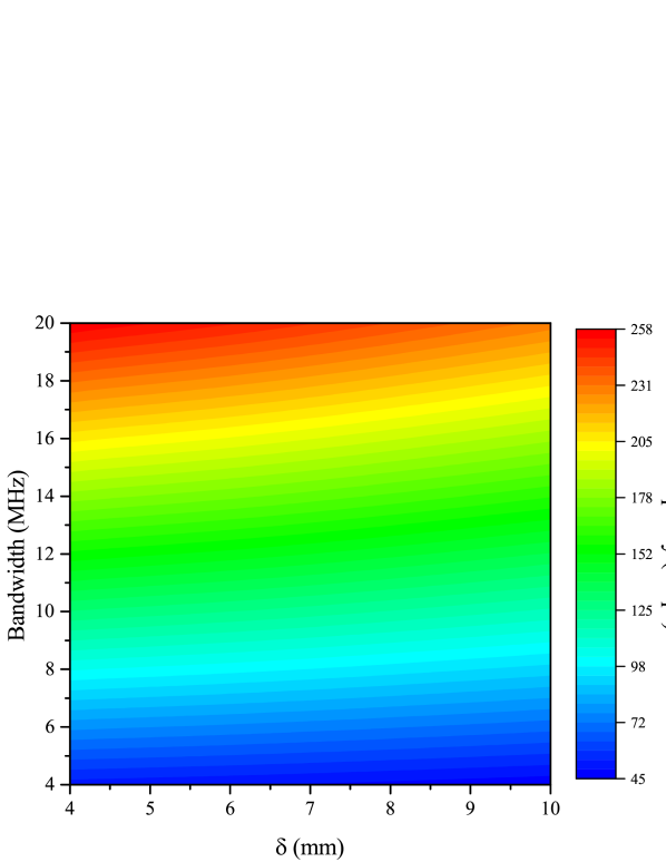
(d) Capacity vs skin thickness and bandwidth.

Figure 2: Impact of skin thickness on the OWCI’s effectiveness.

4.1 Impact of skin thickness

Figure 2(a) demonstrates the impact of skin thickness on the received signal quality in OWCIs operating at different wavelengths. It is observed that the analytical and simulation results coincide, which verifies the accuracy of the derived analytical framework. As expected, as the skin thickness increases for a given wavelength, the average SNR decreases i.e. the received signal quality degrades. For instance, the average SNR degrades by $66.6\%$ at $\lambda=1500\text{ }\mathrm{nm}$ as $\delta$ changes from $4$ to $10\text{ }\mathrm{mm}$, whereas for $\lambda=1100\text{ }\mathrm{nm}$ and the same $\delta$ variation, the average SNR degrades by $13.9\%$. This degradation is caused due to the skin pathloss. Additionally, we observe that for a given skin thickness, $\delta$, the average SNR depends on the wavelength. For example, for $\delta=6$ mm and $\lambda=1450$ nm, the average SNR is $32$ dB, whereas for the same $\delta$ and $\lambda=1500$ nm, the average SNR is $51.3$ dB. Thus, the slight $50$ nm variation of the wavelength from $1450$ to $1500$ nm resulted in a $60\%$ signal quality improvement. On the contrary, when $\lambda$ alters from $400$ nm to $500$ nm, for the same $\delta$, the average SNR increases by $56.5\%$. This observation indicates the wavelength dependency of the TOL as well as the importance of appropriately choosing the wavelength during the OWCI system design phase.

Figure 2(b) illustrates the outage probability as a function of skin thickness for different values of SNR threshold, $\gamma_{\rm th}$, for $\lambda=1500\text{ }\mathrm{nm}$. We observe that for a fixed skin thickness, the outage probability also increases as $\gamma_{\rm th}$ increases. For example, for $\delta=6\text{ }\mathrm{mm}$ and $\gamma_{\rm th}=0.5\text{ }\mathrm{bits/s/Hz}$, the outage probability is about $10^{-5}$, whilst for $\gamma_{\rm th}=4$ and the same $\delta$ it is about $10^{-1}$. Furthermore, for the same $\gamma_{\rm th}$ and when $\delta$ changes from $4\text{ }\mathrm{mm}$ to $6\text{ }\mathrm{mm}$, it is noticed that the outage probability decreases. On the contrary, when $\delta$ exceeds $6\text{ }\mathrm{mm}$ and for the same $\gamma_{\rm th}$, the outage probability increases. This is because the misalignment fading drastically affects the transmission at relatively long TX-RX distances. In other words, as the skin thickness increases, the intensity of the misalignment fading decreases, whereas the impact of pathloss becomes more severe.

Figure 2(c) illustrates the spectral efficiency as a function of the skin thickness and the PSD of the transmission signal. As expected, increasing the transmission signal PSD can countermeasure the impact of skin thickness. For example, for $\delta=8\text{ }\mathrm{mm}$, an increase of the transmission PSD from $0.001\text{ }\mathrm{\mu W/MHz}$ to $0.01\text{ }\mathrm{\mu W/MHz}$ results in a $56.5\%$ increase of the corresponding spectral efficiency. Moreover, we observe that in the worst case scenario, in which the skin thickness is $10\text{ }\mathrm{mm}$, even with particularly low transmission signal PSD of about $0.0001\text{ }\mathrm{\mu W/MHz}$) the achievable spectral efficiency is in the order of $8\text{ }\mathrm{bits/channel\text{ }use}$.

In Fig. 2(d), the channel capacity is depicted as a function of the skin thickness and the bandwidth of the system. As expected, an increase of the bandwidth for the same skin thickness results in an increase of the TOL’s capacity. For instance, as bandwidth increases from $14\text{ }\mathrm{MHz}$ to $18\text{ }\mathrm{MHz}$, for $\delta=6\text{ }\mathrm{mm}$, an improvement of about $28.6\%$ is noticed. In addition, it is observed that even in the worst case scenario in which the bandwidth and the skin thickness are considered $4\text{ }\mathrm{MHz}$ and $10\text{ }\mathrm{mm}$, respectively, the OWCI outperforms the corresponding RF counterparts.

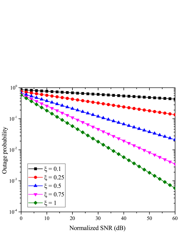
(a) Outage probability vs normalised SNR for different values of $\xi$.

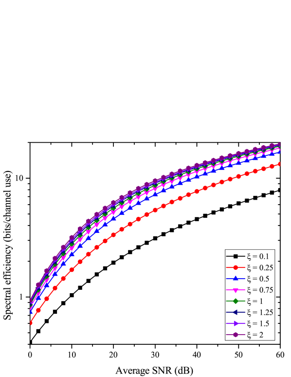
(b) Spectral efficiency vs average SNR for different values of $\xi$.

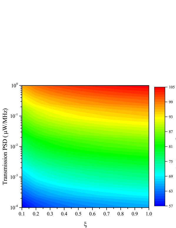
(c) Average SNR vs $\xi$ and transmission PSD.

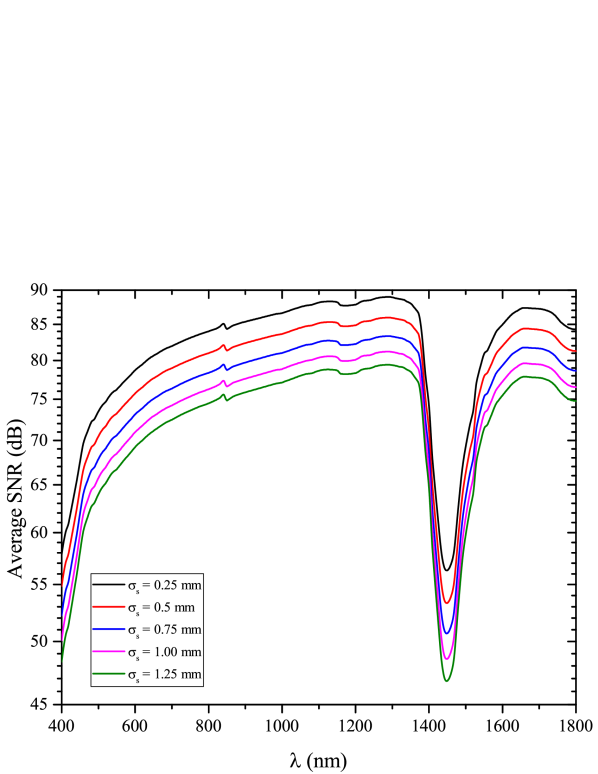
(d) Average SNR vs wavelegth for different values of spatial jitter.

Figure 3: Impact of misalignment on OWCI’s performance.

4.2 Impact of misalignment

In Fig. 3(a), the outage probability is illustrated as a function of the normalized SNR for different values of $\xi$. In this case the normalized SNR is defined as the ratio of the average SNR to the SNR threshold, $\tilde{\gamma}/\gamma_{\rm th}$. Also, markers represent the simulation outcomes whereas the continuous curves represent the corresponding analytical results. It is evident that the analytical results are in agreement with the corresponding simulation results, which verifies the validity of the presented theoretical framework. In addition, we observe that for a fixed normalized SNR, the outage probability increases as the misalignment effect increases, i.e., it is inversely proportional to $\xi$. Moreover, the OWCI performance in terms of outage probability, for a fixed $\xi$, improves, as expected, as the normalized SNR increases. It is also worth noting that as the normalized SNR increases, the misalignment has a more detrimental effect on the outage performance of the OWCI system. For example, for normalized SNR values of $10$ dB and $50$ dB, the outage probability degrades by about $76\%$ and $99.5\%$, respectively, when $\xi$ is changed from $0.1$ to $1$. This indicates the importance of taking the impact of misalignment into consideration when determining the required transmit power and spectral efficiency.

Figure 3(b) demonstrates the impact of misalignment fading on the spectral efficiency of OWCI. Again, markers and continuous curves account for the corresponding simulation and numerical results, respectively. The observed agreement between these results verifies the validity of equation (23). Furthermore, it is noticed that for a given average SNR value, a decrease of $\xi$ constraints the corresponding spectral efficiency. For instance, for an average SNR of $40$ dB, a change of $\xi$ from $2$ to $0.1$ results in a $64.8\%$ spectral efficiency degradation, whereas, for the case of $20\text{ }\mathrm{dB}$, the corresponding spectral efficiency decreases by about  $68.6\%$. This indicates that the impact of misalignment fading is more severe in the high SNR regime. In addition, we observe that the spectral efficiency increases proportionally to the average SNR for fixed values of $\xi$. For example, for $\xi=0.5$ the spectral efficiency increases by $100\%$ and $60\%$, when the average SNR changes from $10$ dB to $20$ dB and from $20$ dB to $30$ dB, respectively. Therefore, it is evident that as the average SNR increases, the spectral efficiency increase is constrained.

Figure 3(c) depicts the average SNR as a function of $\xi$ and $\tilde{P}_{s}$. As expected, for fixed values of $\xi$ the PSD of the transmission signal is proportional to the average SNR. Moreover, for a given $\tilde{P}_{s}$, as the level of alignment increases, i.e. as $\xi$ increases, the average SNR also increases. For example, for $\xi=0.5$, the average SNR increases by about $27.4\%$ as the transmission signal PSD increases from $0.001\text{ }\mathrm{\mu W/MHz}$ to $0.1\text{ }\mathrm{\mu W/MHz}$. Additionally, we observe that for $\tilde{P}_{s}=0.001\text{ }\mathrm{\mu W/MHz}$, the average SNR increases by a factor of $3.2\%$ as $\xi$ increases from $0.4$ to $0.8$. This indicates that the misalignment fading affects the average SNR more subtly than the transmission signal PSD. Finally, it becomes evident that the impact of misalignment fading can be countermeasured by increasing the PSD of the transmission signal.

Figure 3(d), demonstrates the average SNR as a function of the operating wavelength for different values of the jitter SD, $\sigma_{s}$. As expected, for a given wavelength, as the intensity of the misalignment fading increases i.e. as the jitter SD increases, the signal quality degrades and thus the average SNR decreases. It is also noticed that the optimal operation wavelength, which maximizes the average SNR, is $1100\text{ }\mathrm{nm}$ whereas the worst performance is achieved at lower wavelengths than $600\text{ }\mathrm{nm}$ and around $1450\text{ }\mathrm{nm}$. In addition, a suboptimal operation wavelength is around $1300\text{ }\mathrm{nm}$, while it is shown that there is an ultra wideband transmission window from $700$ nm to $1300\text{ }\mathrm{nm}$. It is worth noting that several commercial optical units (i.e. LEDs and PDs) exist in this particular window.

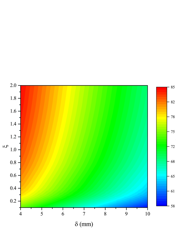
(a) Average SNR vs skin thickness and $\xi$, for $\lambda=940\text{ }\mathrm{nm}$.

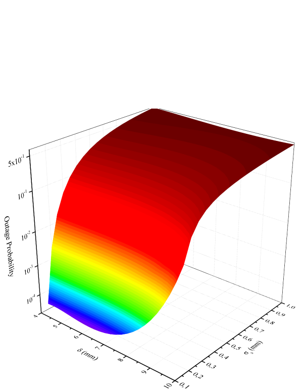
(b) Outage probability vs skin thickness and jitter SD.

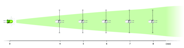
(c) Illustration of the misalignment fading as a function of the skin thickness.

Figure 4: The joint effect of skin thickness and misalignment.

4.3 Joint effect of skin thickness and misalignment

Figure 4(a) illustrates the joint effect of skin thickness and misalignment fading in the received signal quality in terms of the average SNR and for a wavelength of $940$ nm. It is evident that for fixed values of $\xi$, the average SNR decreases as the skin thickness increases. For instance, for $\xi=0.5$, the SNR decreases by $13.8\%$ as the skin thickness increases from $5$ mm to $9$ mm, whereas for $\xi=2$, the SNR decreases by $13.1\%$, for the same skin thickness variation. This indicates that the average SNR degradation due to skin thickness increase depends on the intensity of the misalignment fading. In addition, we observe that for a fixed skin thickness and as $\xi$ increases i.e. the intensity of misalignment fading decreases, the average SNR also increases. For example, for $\delta=7$ mm and when $\xi$ changes from $0.1$ to $1.5$, the average SNR increases by about $10\text{ }\mathrm{dB}$, from $65.9\text{ }\mathrm{dB}$ to $75.44\text{ }\mathrm{dB}$. Finally, it is noticed that for practical values of $\delta$ and $\xi$, i.e. $\delta\in[4,10]\text{ }\mathrm{mm}$ and $\xi\in[0.1,2]$, the achievable average SNR is particularly high, despite the low transmission signal PSD.

In Fig. 4(b), the outage probability is demonstrated as a function of the skin thickness and the jitter SD. It is evident that the impact of misalignment fading in the low $\delta$ regime is more detrimental than in the high regime. This is expected since, as illustrated in Fig. 4(c) and for a fixed spatial jitter, the skin thickness is proportional to the probability that the RX is within the transmission effective area. However, as $\delta$ increases the pathloss also increases, which shows that the impact of misalignment fading is more severe than the effect of pathloss for realistic values of skin thickness.

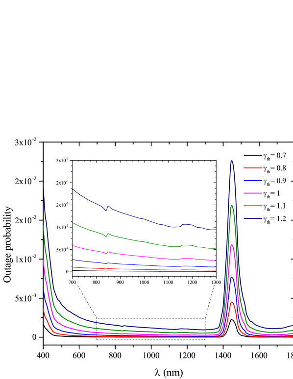
(a) Outage probability vs wavelegth for different values of SNR threshold.

(b) Ergodic capacity vs wavelength and skin thickness, assuming heterodyne RX.

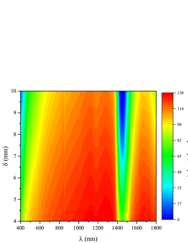
(c) Ergodic capacity lower bound vs wavelength and skin thickness, assuming IM/DD RX.

Figure 5: The impact of channel wavelength selectivity on the performance of OWCIs.

4.4 Design parameters

In this section, we present the impact of different design selections in the effectiveness of OWCIs in terms of the average SNR, ergodic spectral efficiency and channel capacity. The investigated design parameters are related to the transmission LED and PD physical characteristics.

4.4.1 Selecting the appropriate wavelength

Figure 5(a) depicts the outage probability as a function of the wavelength for different values of the SNR threshold, assuming $\xi=1$ and a transmission signal PSD of $0.1\text{ }\mathrm{\mu W/MHz}$. Moreover, the outage probability is, as expected, proportional to $\gamma_{\rm th}$ for fixed wavelength values. For example, for the case of $\lambda=600\text{ }\mathrm{nm}$ the outage probability increases approximately by $150\%$ as $\gamma_{\rm th}$ is changed from $0.8$ to $0.9$. Likewise, it is evident that a transmission window exists for wavelengths between $700$ nm and $1300\text{ }\mathrm{nm}$. It is worth noting that several commercial LEDs and PDs exist in this wavelength range (see for example[50, 51, 52, 53, 54]). Finally, we observe that the wavelength windows from $400$ nm to $600\text{ }\mathrm{nm}$ and around $1450\text{ }\mathrm{nm}$ are not optimal for OWCIs, since the optimal transmission wavelength is $1100\text{ }\mathrm{nm}$.

In Fig. 5(b), the ergodic capacity of the TOL is demonstrated as a function of the wavelength and the skin thickness, under the assumption of heterodyne RX. Although the transmit power and the bandwidth are relatively low, OWCI can achieve a capacity in the range between $1\text{ }\mathrm{Mbps}$ and $136\text{ }\mathrm{Mbps}$. In addition, we observe that for a fixed wavelength the skin thickness increases as the capacity decreases. For instance, for the case of $\lambda=500\text{ }\mathrm{nm}$ the capacity degrades by $10.3\%$ and $12.3\%$ as the skin thickness increases from $5$ mm to $7\text{ }\mathrm{mm}$ and from $7$ mm to $9\text{ }\mathrm{mm}$, respectively. Likewise, the same skin thickness alterations for $\lambda=1100\text{ }\mathrm{nm}$ result to a respective capacity degradation of $3.3\%$ and $4\%$. Furthermore, for the same skin thickness alterations and $\lambda=1450\text{ }\mathrm{nm}$, the capacity degrades by $49.5\%$ and $85\%$, respectively. This indicates that the level of the capacity degradation due to the skin thickness depends largely on the corresponding wavelength value. Moreover, it is evident that the optimal performance in terms of spectral efficiency is achieved at a wavelength around $1100\text{ }\mathrm{nm}$, independently of the skin thickness. In this particular wavelength, the minimum and maximum achievable ergodic capacities are $120.87\text{ }\mathrm{Mbps}$ and $135\text{ }\mathrm{Mbps}$, respectively. On the contrary, for $\delta\leq 5.25\text{ }\mathrm{nm}$ the worst possible capacity is achieved at $\lambda=400\text{ }\mathrm{nm}$, whereas for $\delta>5.25\text{ }\mathrm{nm}$ it is achieved at $\lambda=1450\text{ }\mathrm{nm}$. Furthermore, we observe that the optimal transmission window ranges between $\lambda=900$ nm and $\lambda=1300\text{ }\mathrm{nm}$.

Similarly, the ergodic capacity lower bound is illustrated in Fig. 5(c) as a function of the wavelength and the skin thickness, assuming IM/DD RX. By comparing the results in Fig. 5(b) and 5(c), we observe that in both cases the optimal, the sub-optimal and the worst transmission wavelengths coincide. Also, it is evident that regardless of the type of the RX, the optimal transmission window is in the range between $\lambda=900$ nm and $\lambda=1300\text{ }\mathrm{nm}$. In other words, the comparison of these figures reveals that the selection of the transmission wavelength should be independent of the RX type.

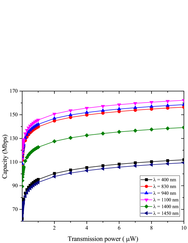
(a) Ergodic capacity vs transmit power for different wavelengths.

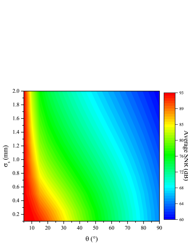
(b) Average SNR vs divergence angle and jitter SD.

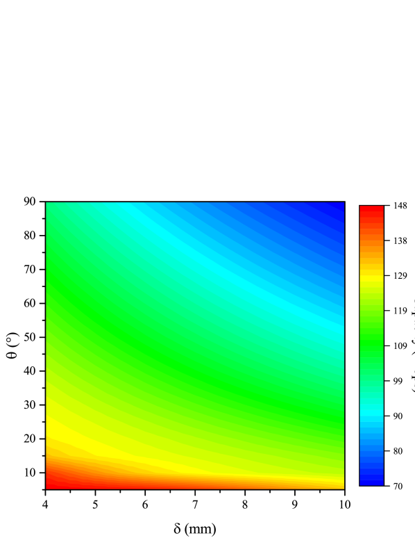
(c) Ergodic capacity vs skin thickness and divergence angle.

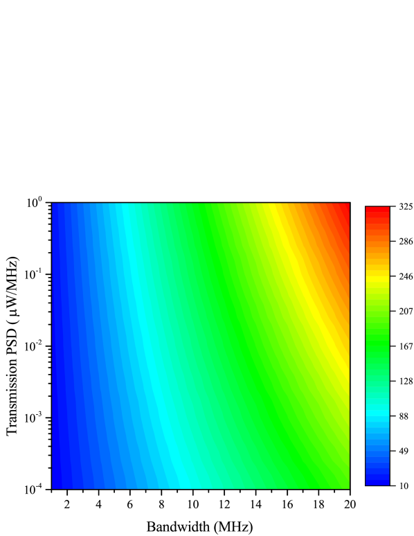
(d) Ergodic capacity lower bound vs bandwidth and transmit power.

Figure 6: The impact of TX design parameters on the performance of OWCI.

4.4.2 TX parameters

In Fig. 6(a), the capacity of the TOL is depicted as a function of the transmit power at different wavelengths. The considered wavelengths correspond to the best case scenario, which occurs at the optimal wavelength of the OWCI ($1100\text{ }\mathrm{nm}$), the worst case scenario based on the skin attenuation coefficient ($1450\text{ }\mathrm{nm}$), the worst case scenario based on the responsivity of the photodetector ($400\text{ }\mathrm{nm}$), two cases of wavelengths commonly used in commercial LEDs ($830\text{ }\mathrm{nm}$ and $940\text{ }\mathrm{nm}$), and one scenario for an intermediate value ($1400\text{ }\mathrm{nm}$). To this end, we observe that the maximum capacity is achieved at $1100\text{ }\mathrm{nm}$, while at $830$ nm, where the TSHG5510 operates [50], and $940\text{ }\mathrm{nm}$, where the IR333 [51] operates, the received capacity approaches the optimum. This indicates that commercial optics can be effectively used in the development of OWCIs. Interestingly, the worst case scenario at $1450\text{ }\mathrm{nm}$ provides slightly higher capacity than the one at $400\text{ }\mathrm{nm}$. As a result, we observe that both the PD’s responsivity and the skin transmitivity drastically impact the quality of the OWCI link. Also, even though the transmit signal power of the OWCI is considerably lower compared to the RF counterpart (in the order of $40\text{ }\mathrm{mW}$ [2, 55]), the achievable data rate of the OWCI is surprisingly high, i.e. in the order of $150\text{ }\mathrm{Mbps}$. This indicates that the OWCI can achieve a substantially higher power and data rate efficiency compared to the corresponding conventional RF system.

In Fig. 6(b), the average SNR is illustrated as a function of the TX’s divergence angle and the jitter SD. We observe that the value of average SNR decreases at an increase of the divergence angle and the jitter SD. For instance, for $\theta=20^{o}$, as jitter SD increases from $0.1\text{ }\mathrm{mm}$ to $1\text{ }\mathrm{mm}$, the average SNR increases by $10.22\%$. In addition, it is noticed that for a fixed $\sigma_{s}=0.5\text{ }\mathrm{mm}$ the average SNR increases by about $9.8\%$ as the divergence angle varies from $10^{o}$ to $30^{o}$. This indicates that by employing LEDs with low divergence angle, we can countermeasure the impact of misalignment fading.

In Fig. 6(c), the ergodic capacity is illustrated as a function of the skin thickness and the divergence angle, assuming heterodyne RX. It is shown that for a fixed $\theta$, the capacity decreases as $\delta$ increases. For example, for $\theta=15^{o}$ and $\delta=5\text{ }\mathrm{mm}$, a $128.77\text{ }\mathrm{Mbps}$ ergodic capacity is achieved, whereas for the same $\theta$ and $\delta=10\text{ }\mathrm{mm}$, the ergodic capacity is $119.43\text{ }\mathrm{Mbps}$. Therefore, a $7.25\%$ ergodic capacity degradation occurs when the skin thickness doubles. On the contrary, for a given $\delta$ the capacity is inversely proportional to $\theta$; hence, we observe that by decreasing the divergence angle, we can countermeasure the incurred pathloss effect. For instance, for the case of $\delta=8\text{ }\mathrm{mm}$, a $5\%$ capacity increase is achieved when the divergence angle changes from $20^{o}$ to $10^{o}$.

Figure 6(d), depicts the capacity of the TOL as a function of the transmission bandwidth and PSD. As expected, for a fixed transmission PSD the capacity of the system improves as the available bandwidth increases. For example, for $\tilde{P_{s}}=0.001\text{ }\mathrm{\mu W/MHz}$, the capacity improves by approximately $200\%$ as the bandwidth increases from $6\text{ }\mathrm{MHz}$ to $18\text{ }\mathrm{MHz}$. In addition, we observe that for a certain bandwidth, an increase of the transmission PSD improves the system capacity by a lesser factor. For instance, when the bandwidth is $10\text{ }\mathrm{MHz}$ and transmission PSD increases from $0.001\text{ }\mathrm{\mu W/MHz}$ to $0.1\text{ }\mathrm{\mu W/MHz}$, the TOL’s capacity also increases by a factor of $29.6\%$. This indicates that the bandwidth affects the quality of the TOL more severely than the transmission PSD.

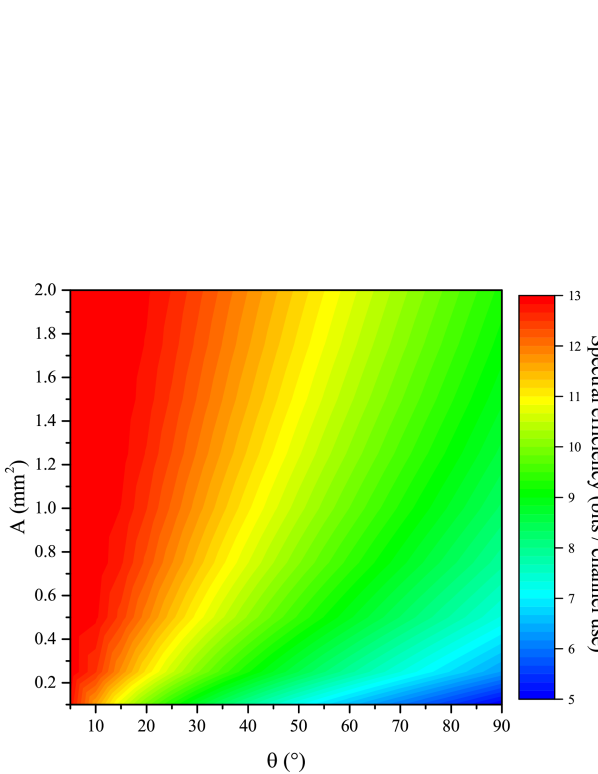
(a) Spectral efficiency vs PD effective area and divergence angle.

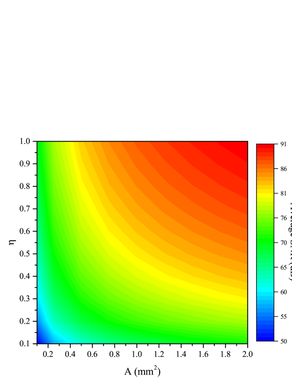
(b) Average SNR vs PD effective area and photodiode’s quantum efficiency.

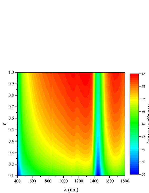
(c) Average SNR vs wavelength and PD’s quantum efficiency.

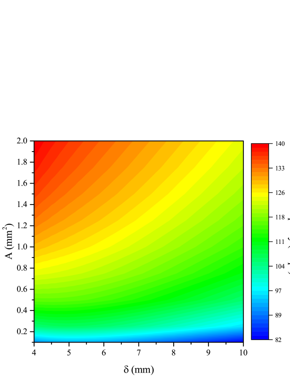
(d) Ergodic capacity vs skin thickness and PD effective area.

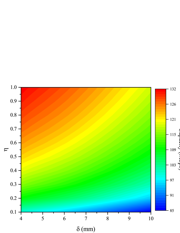
(e) Ergodic capacity vs skin thickness and quantum efficiency.

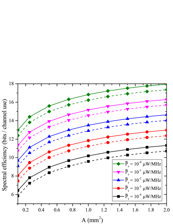
(f) Spectral efficiency vs photodiode effective area for different values of transmissioin PSD, heterodyne (continious lines) and IM/DD (dashed lines) RX.

Figure 7: The impact of RX design parameters on the performance of OWCI.

4.4.3 RX parameters

This section discusses the impact of the physical characteristics of the RX optical unit. To this end, Fig. 7(a) exhibits the proportionality of the spectral efficiency with respect to the effective area, $A$, of the PD for a given divergence angle, $\theta$. For instance, a $24.9\%$ spectral efficiency increase can be achieved at $\theta=20^{\circ}$ by increasing the PD’s effective area from $0.1\text{ }\mathrm{mm}^{2}$ to $1\text{ }\mathrm{mm}^{2}$. On the contrary, the spectral efficiency is inversely proportional to $\theta$ for a fixed $A$. For example, a $11.4\%$ spectral efficiency degradation occurs for $A=1\text{ }\mathrm{mm}^{2}$ when $\theta$ increases from $20^{o}$ to $40^{o}$.

Figure 7(b) depicts the average SNR as a function of the PD’s effective area and quantum efficiency, $\eta$. We observe that the value of average SNR increases as A and $\eta$ increase. For example, for $\eta=0.3$ and $A=0.5\text{ }\mathrm{mm^{2}}$ the average SNR is approximately $71.86\text{ }\mathrm{dB}$, while for the same $\eta$ and $A=1.5\text{ }\mathrm{mm^{2}}$, it is approximately $79.12\text{ }\mathrm{dB}$. In addition, in the case of $A=1\text{ }\mathrm{mm^{2}}$ and $\eta=0.2$, the average SNR is approximately $73.1\text{ }\mathrm{dB}$, whilst for the same $A$ and $\eta=0.8$, it is approximately $85.15\text{ }\mathrm{dB}$.

Figure 7(c) presents the average SNR as a function of the wavelength and the PD’s quantum efficiency. We observe that the OWC link achieves an average SNR in the range between $35$ dB and $88\text{ }\mathrm{dB}$. In addition, the PD’s quantum efficiency is, as expected, proportional to the average SNR for a fixed wavelength. Also, as analyzed in Fig. 3(d), it becomes evident that a transmission window exists for wavelengths between $700\text{ }\mathrm{nm}$ and $1300\text{ }\mathrm{nm}$, where the link achieves the highest values for the average SNR. Furthermore, for the optimal value at $\lambda=1100\text{ }\mathrm{nm}$, as $\eta$ increases from $0.2$ to $0.8$ the average SNR increases by $16.5\%$. This indicates that the selection of the operation wavelength is more critical than the quantum efficiency of the PD.

Figure 7(d) illustrates the ergodic capacity as a function of the skin thickness and the effective area of the PD. It is noticed that regardless of the values of $\delta$ and $A$, the ergodic capacity is in the range between $82$ Mbps and $140$ Mbps, which is substantially higher than the achievable rate in the baseline RF CI solution that does not exceed $1\text{ }\mathrm{Mbps}$ [2, 55]. As expected, as $\delta$ increases for a fixed $A$, the pathloss increases and therefore the capacity decreases. For instance, as $\delta$ increases from $5\text{ }\mathrm{mm}$ to $9\text{ }\mathrm{mm}$, for $A=1\text{ }\mathrm{mm}^{2}$, the capacity of the system decreases by a factor of $7.4\%$. On the contrary, the ergodic capacity also increases as $A$ increases, for a given $\delta$. For example, for $\delta=6\text{ }\mathrm{mm}$, the ergodic capacity increases by $88.7\%$ when $A$ varies from $0.5\text{ }\mathrm{mm}^{2}$ to $1.5\text{ }\mathrm{mm}^{2}$. In other words, an increase on the PD’s effective area can countermeasure the pathloss effect.

In Fig. 7(e), we demonstrate the joint effect of the PD’s quantum efficiency and skin thickness on the OWCI performance in terms of the ergodic capacity. It is evident that increasing the quantum efficiency can prevent the capacity loss due to the skin thickness. For example, a PD with $\eta=0.3$ achieves an ergodic capacity of $114.86\text{ }\mathrm{Mbps}$ for $\delta=4\text{ }\mathrm{mm}$, whilst a similar performance can be achieved for $\eta=0.7$ when the skin thickness is $9\text{ }\mathrm{mm}$.

In Fig. 7(f), we illustrate the impact of the PD effective area on the corresponding spectral efficiency for different values of transmission PSD and different type of RXs, namely heterodyne and IM/DD. As anticipated, the spectral efficiency is proportional to $\tilde{P}_{s}$ for a fixed PD effective area. Moreover, for a given $\tilde{P}_{s}$, as the PD effective area increases, the spectral efficiency also increases. For instance, for $\tilde{P}_{s}=1\text{ }\mathrm{\mu W/MHz}$ and heterodyne RX, the spectral efficiency increases by $7.9\%$ when the PD effective area changes from $0.5\text{ }\mathrm{mm}^{2}$ to $1\text{ }\mathrm{mm}^{2}$, whereas from the same signal PSD a PD with an effective area of $1.5\text{ }\mathrm{mm}^{2}$ can achieve $4.12\%$ higher spectral efficiency compared to a PD with effective area of $1\text{ }\mathrm{mm}^{2}$. This indicates that as the PD effective area increases, the spectral efficiency gain is not linearly increased. Finally, we observe that for a given signal PSD and PD effective area, the heterodyne RX outperforms the corresponding IM/DD RX. For example, for $\tilde{P}_{s}=1\text{ }\mathrm{\mu W/MHz}$ and $A=1\text{ }\mathrm{mm}^{2}$, the use of IM/DD instead of heterodyne RX reduces the spectral efficiency by about $3.6\%$. However, it is worth noting that IM/DD exhibits considerably lower complexity compared to the corresponding heterodyne RX.

5 Conclusion

The above findings revealed that OWCIs outperforms the corresponding baseline CIs in terms of received signal quality, outage performance, spectral efficiency and channel capacity. In addition, they require significantly less transmit power, which renders them highly energy efficient. Notably, this difference in required power is about three orders of magnitude, since OWCI can achieve Mbps capacity levels with only few $\mu$W, contrary to conventional RF based CIs that require at least few mW to achieve this capacity. Furthermore, another advantage of OWCIs in comparison with RF based CI solutions is that they operate in a non-standardized frequency region, where there is a significantly large amount of unexploited bandwidth; as a result, there is no interference from other medical implanted devices. Therefore, it is evident that all these factors constitute OWCI a particularly attractive alternative to the RF CI solution.

Appendices

Appendix A

Proof of Theorem 1

According to (11), the instantaneous SNR is a random variable (RV) that follows the same distribution as $h_{p}^{2}$. Therefore, in order to derive the average SNR of the optical link, we first need to identify the distribution of $h_{p}^{2}$.

By assuming that the spatial intensity of $w_{\rm\delta}$ on the RX plane at distance $\delta$ from the TX and circular aperture of radius $\beta$, the stochastic term of the channel coefficient, which represents the fraction of the collected power due to geometric spread with radial displacement $r$ from the origin of the detector, can be approximated as

$$h_{p}\approx A_{0}\exp\left(-\frac{2r^{2}}{w_{\rm eq}^{2}}\right).$$ (37)

This is a well-known approximation that has been used in several reported contributions (see for example [45, 56], and references therein).

Moreover, by assuming that the elevation and the horizontal displacement (sway) follow independent and identical Gaussian distributions and based on [35],we observe that the radial displacement at the RX follows a Rayleigh distribution with a probability density function (PDF) given by [57]

$$f_{r}\left(r\right)=\frac{r}{\sigma_{s}^{2}}\exp\left(-\frac{r^{2}}{2\sigma_{s}^{2}}\right),\qquad r>0$$ (38)

By combining (37) and (38), the PDF of $h_{p}$ can be expressed as

$$f_{\rm h_{p}}\left(x\right)=\frac{\xi}{A_{0}^{\xi}}x^{\xi-1},\qquad 0\leq x\leq A_{0}$$ (39)

while, its cumulative distribution function (CDF) can be obtained as

$$F_{\rm h_{p}}\left(x\right)\triangleq\int_{0}^{x}\!f_{\rm y}\left(x\right)\,\mathrm{d}y$$ (40)

which upon substituting (39) in (40) and performing the integration yields

$$F_{\rm h_{p}}\left(x\right)=\left\{\begin{array}[]{c c}\frac{1}{A_{0}^{\xi}}x^{\xi}&0\leq x\leq A_{0}\\ 1,&x\geq A_{0}\end{array}\right.$$ (43)

The CDF of $h_{p}^{2}$ can be obtained as

$$F_{\rm h_{p}^{2}}\left(x\right)=P\left(h_{p}^{2}\leq x\right)=P\left(h_{p}\leq\sqrt{x}\right)=P\left(h_{p}\leq\sqrt{x}\right)=F_{\rm h_{p}}\left(\sqrt{x}\right)$$ (44)

which, by using (43), can be rewritten as

$$F_{\rm h_{p}^{2}}\left(x\right)=\left\{\begin{array}[]{c c}\frac{1}{A_{0}^{\xi}}x^{{\xi}/{2}}&0\leq x\leq A_{0}^{2}\\ 1,&x\geq A_{0}^{2}\end{array}\right..$$ (47)

Moreover, the PDF of $h_{p}^{2}$ can be obtained as

$$f_{\rm h_{p}^{2}}\left(x\right)=\frac{\mathrm{d}F_{\rm h_{p}^{2}}\left(x\right)}{\mathrm{d}x}$$ (48)

or, by employing (47) as

$$f_{\rm h_{p}^{2}}\left(x\right)=\frac{\xi}{2A_{0}^{\xi}}x^{\frac{\xi}{2}-1}.$$ (49)

Finally, the average SNR can be defined as

$$\tilde{\gamma}=\mathbb{E}[\gamma].$$ (50)

Thus, by substituting (11) into (50), and using (49), we obtain

$$\tilde{\gamma}=\frac{R\exp\left(-\alpha(\lambda)\delta\right)\tilde{P}_{s}}{2qRP_{b}+2qI_{\rm DC}+N_{0}}\frac{\xi}{2A_{0}^{\xi}}\int_{0}^{A_{0}^{2}}x^{\frac{\xi}{2}}\mathrm{d}x$$ (51)

which, by performing the integration yields (12), which concludes the proof.

Appendix B

Proof of Theorem 2

By assuming full knowledge of the channel state information (CSI) at both the TX and the RX, the ergodic spectral efficiency, C, (in $\mathrm{bits/channel\text{ }use}$) can be obtained by [47, eq. (7.43)], [58, eq. (9.40)] and  [59, 60, 61, 32, 62, 63, 64, 65, 66, 67, 68, 69], namely

$$C=\frac{1}{2}\mathbb{E}\left[\log_{2}\left(1+\psi\gamma\right)\right]$$ (52)

where

$$\psi=\left\{\begin{array}[]{c c}1,&\text{for heterodyne RX}\\ \tfrac{e}{2\pi},&\text{for IM/DD RX}\end{array}\right.$$ (55)

or equivalently

$$C=\frac{1}{2}\int_{\rm 0}^{A}\log_{2}\left(1+\psi\frac{R^{2}\exp\left(-\alpha(\lambda)\delta\right)x^{2}\tilde{P}_{s}}{2qRP_{b}+2qI_{\rm DC}+N_{0}}\right)f_{\rm h_{p}}(x)\mathrm{d}x.$$ (56)

By substituting (39) into (56) and after some algebraic manipulations, equation (56) is given by

$$C=\frac{\xi}{2A_{0}^{\xi}\ln\left(2\right)}\mathcal{I}$$ (57)

where

$$\mathcal{I}=\int_{\rm 0}^{A_{0}}x^{\xi-1}\ln(1+\mathcal{B}(\lambda)x^{2})\mathrm{d}x$$ (58)

or

$$\mathcal{I}=\frac{1}{\xi}\int_{\rm 0}^{A_{0}}\ln(1+\mathcal{B}(\lambda)x^{2})\frac{\mathrm{d}x^{\xi}}{\mathrm{d}x}\mathrm{d}x.$$ (59)

By applying integration by parts into (59), we obtain

$$\mathcal{I}=\frac{1}{\xi}A_{0}^{\xi}\ln\left(1+\mathcal{B}(\lambda)A_{0}^{2}\right)-\frac{1}{\xi}\int_{0}^{A_{0}}\frac{x^{\xi}}{1+\mathcal{B}(\lambda)x^{2}}\mathrm{d}x$$ (60)

which, by using [29], can be expressed as

$$\mathcal{I}=\frac{1}{\xi}A_{0}^{\xi}\ln\left(1+\mathcal{B}(\lambda)A_{0}^{2}\right)-\frac{1}{\xi}A_{0}^{\xi+2}\mathcal{B}(\lambda)\Phi\left(A_{0}^{2}\mathcal{B}(\lambda),1,1+\frac{\xi}{2}\right).$$ (61)

Finally, by substituting (61) into (57), and after some mathematical manipulations, we obtain (17), which concludes the proof.

Appendix C

Proof of Proposition 1

It is recalled that the Lerch-$\Phi$ function can be expressed in integral form as

$$\Phi(a,b,x)\triangleq\frac{1}{\Gamma(b)}\int_{0}^{\infty}\frac{y^{b-1}e^{-xy}}{1-ae^{-y}}\mathrm{d}y.$$ (62)

Based on this and recalling that $\Gamma(1)\triangleq 0!$, it immediately follows that

$$C=\frac{1}{2}\log_{2}\left(1+\mathcal{B}(\lambda)A_{0}^{2}\right)-\frac{1}{2}\frac{A_{0}^{2}\mathcal{B}(\lambda)}{\ln(2)}\int_{0}^{\infty}\frac{e^{-\left(1+\frac{\xi}{2}\right)y}}{1+A_{0}^{2}\mathcal{B}(\lambda)e^{-y}}\mathrm{d}y.$$ (63)

Notably, $1+A_{0}^{2}\mathcal{B}(\lambda)e^{-y}>A_{0}^{2}\mathcal{B}(\lambda)e^{-y}$, which when $A_{0}^{2}\mathcal{B}>>1$ becomes $1+A_{0}^{2}\mathcal{B}(\lambda)e^{-y}\simeq A_{0}^{2}\mathcal{B}(\lambda)e^{-y}$. To this end, equation (64) cen be lower bounded as follows:

$$C>\frac{1}{2}\log_{2}\left(1+\mathcal{B}(\lambda)A_{0}^{2}\right)-\frac{1}{2}\frac{A_{0}^{2}\mathcal{B}(\lambda)}{\ln(2)}\int_{0}^{\infty}\frac{e^{-\left(1+\frac{\xi}{2}\right)y+y}}{A_{0}^{2}\mathcal{B}(\lambda)}\mathrm{d}y.$$ (64)

Therefore, by evaluating the above basic integral and after some algebraic manipulations one obtains (19), which concludes the proof.

Appendix D

Proof of Theorem 3

We recall that the outage probability is defined as the probability that the achievable spectral efficiency, $C$, falls below a predetermined threshold, $r_{\rm th}$, i.e.

$$P_{o}(r_{\rm th})=P_{\rm r}(C\leq r_{\rm th})=P_{\rm r}(\gamma\leq\gamma_{\rm th})$$ (65)

where $r_{\rm th}$ and $\gamma_{\rm th}$ represent the data rate threshold and the SNR threshold, respectively, whereas

$$\gamma_{\rm th}=\frac{2^{2r_{\rm th}}-1}{\psi}.$$ (66)

Thus, with the aid of (11), equation (65) can be rewritten as

$$P_{o}(\gamma_{\rm th})=P_{\rm r}\left(h_{p}^{2}\leq\frac{2qRP_{b}+2qI_{\rm DC}+N_{0}}{R^{2}\exp\left(-\alpha(\lambda)\delta\right)\tilde{P}_{s}}\gamma_{\rm th}\right)=F_{\rm h_{p}^{2}}\left(\frac{2qRP_{b}+2qI_{\rm DC}+N_{0}}{R^{2}\exp\left(-\alpha(\lambda)\delta\right)\tilde{P}_{s}}\gamma_{\rm th}\right)$$ (67)

where $F_{\rm h_{p}^{2}}\left(\cdot\right)$ denotes the cumulative distribution function (CDF) of the stochastic process $h_{p}^{2}$, and can be deduced from (39). As a result, (65) can be rewritten in closed-form as in (28), which concludes the proof.

Funding

Khalifa University of Science and Technology (8474000122, 8474000137).

Disclosures

The authors declare that there are no conflicts of interest related to this article.

References

- [1] B. S. Wilson, “The modern cochlear implant: A triumph of biomedical engineering and the first substantial restoration of human sense using a medical intervention,” \JournalTitleIEEE Pulse 8, 29–32 (2017).
- [2] F. G. Zeng, S. Rebscher, W. Harrison, X. Sun, and H. Feng, “Cochlear implants: System design, integration, and evaluation,” \JournalTitleIEEE Rev. Biomed. Eng. 1, 115–142 (2008).
- [3] I. Hochmair, P. Nopp, C. Jolly, M. Schmidt, H. Schößer, C. Garnham, and I. Anderson, “MED-EL cochlear implants: State of the art and a glimpse into the future,” \JournalTitleTrends Amplif. 10, 201–219 (2006).
- [4] J. F. Patrick, P. A. Busby, and P. J. Gibson, “The development of the nucleus® freedom cochlear implant system,” \JournalTitleTrends Amplif. 10, 175–200 (2006).
- [5] K. Agarwal, R. Jegadeesan, Y. X. Guo, and N. V. Thakor, “Wireless power transfer strategies for implantable bioelectronics,” \JournalTitleIEEE Rev. Biomed. Eng. 10, 136–161 (2017).
- [6] H. J. Kim, H. Hirayama, S. Kim, K. J. Han, R. Zhang, and J. W. Choi, “Review of near-field wireless power and communication for biomedical applications,” \JournalTitleIEEE Access 5, 21264–21285 (2017).
- [7] A. C. Thompson, S. A. Wade, N. C. Pawsey, and P. R. Stoddart, “Infrared neural stimulation: Influence of stimulation site spacing and repetition rates on heating,” \JournalTitleIEEE Trans. Biomed. Eng. 60, 3534–3541 (2013).
- [8] W. H. Ko, “Early history and challenges of implantable electronics,” \JournalTitleJ. Emerg. Technol. Comput. Syst. 8, 1–9 (2012).
- [9] M. N. Islam and M. R. Yuce, “Review of medical implant communication system (MICS) band and network,” \JournalTitleICT Express 2, 188–194 (2016).
- [10] T. Liu, U. Bihr, S. M. Anis, and M. Ortmanns, “Optical transcutaneous link for low power, high data rate telemetry,” in Annual International Conference of the IEEE Engineering in Medicine and Biology Society (EMBC), (IEEE, 2012), pp. 3535–3538.
- [11] S. L. Pinski and R. G. Trohman, “Interference in implanted cardiac devices, part i,” \JournalTitlePacing Clin. Electrophysiol 25, 1367–1381 (2002).
- [12] Z. Ghassemlooy, S. Arnon, M. Uysal, Z. Xu, and J. Cheng, “Emerging optical wireless communications-advances and challenges,” \JournalTitleIEEE J. Sel. Areas Commun. 33, 1738–1749 (2015).
- [13] Z. Ghassemlooy, L. N. Alves, S. Zvanovec, and M.-A. Khalighi, Visible Light Communications: Theory and Applications (CRC Press, 2017).
- [14] M. Z. Chowdhury, M. T. Hossan, A. Islam, and Y. M. Jang, “A comparative survey of optical wireless technologies: Architectures and applications,” \JournalTitleIEEE Access 6, 9819–9840 (2018).
- [15] J. L. Abita and W. Schneider, “Transdermal optical communications,” \JournalTitleJohns Hopkins APL Tech. Dig. 25, 261 (2004).
- [16] D. M. Ackermann, B. Smith, K. L. Kilgore, and P. H. Peckham, “Design of a high speed transcutaneous optical telemetry link,” in Engineering in Medicine and Biology Society, 2006. EMBS’06. 28th Annual International Conference of the IEEE, (IEEE, 2006), pp. 2932–2935.
- [17] D. M. Ackermann Jr, B. Smith, X.-F. Wang, K. L. Kilgore, and P. H. Peckham, “Designing the optical interface of a transcutaneous optical telemetry link,” \JournalTitleIEEE Trans. Biomed. Eng. 55, 1365–1373 (2008).
- [18] Y. Gil, N. Rotter, and S. Arnon, “Feasibility of retroreflective transdermal optical wireless communication,” \JournalTitleAppl. Opt. 51, 4232–4239 (2012).
- [19] T. Liu, J. Anders, and M. Ortmanns, “System level model for transcutaneous optical telemetric link,” in IEEE International Symposium on Circuits and Systems (ISCAS), (IEEE, 2013), pp. 865–868.
- [20] T. Liu, U. Bihr, J. Becker, J. Anders, and M. Ortmanns, “In vivo verification of a 100 mbps transcutaneous optical telemetric link,” in IEEE Biomedical Circuits and Systems Conference (BioCAS), (IEEE, 2014), pp. 580–583.
- [21] T. Liu, J. Anders, and M. Ortmanns, “Bidirectional optical transcutaneous telemetric link for brain machine interface,” \JournalTitleElectron. Lett. 51, 1969–1971 (2015).
- [22] E. Okamoto, Y. Yamamoto, Y. Inoue, T. Makino, and Y. Mitamura, “Development of a bidirectional transcutaneous optical data transmission system for artificial hearts allowing long-distance data communication with low electric power consumption,” \JournalTitleJ. Artif. Organs 8, 149–153 (2005).
- [23] K. Duncan and R. Etienne-Cummings, “Selecting a safe power level for an indoor implanted uwb wireless biotelemetry link,” in IEEE Biomedical Circuits and Systems Conference (BioCAS), (2013), pp. 230–233.
- [24] C. Goßler, C. Bierbrauer, R. Moser, M. Kunzer, K. Holc, W. Pletschen, K. Köhler, J. Wagner, M. Schwaerzle, P. Ruther, O. Paul, J. Neef, D. Keppeler, G. Hoch, T. Moser, and U. T. Schwarz, “GaN-based micro-LED arrays on flexible substrates for optical cochlear implants,” \JournalTitleJ. Phys. D: Appl. Phys. 47, 205401 (2014).
- [25] N. Kallweit, P. Baumhoff, A. Krueger, N. Tinne, A. Kral, T. Ripken, and H. Maier, “Optoacoustic effect is responsible for laser-induced cochlear responses,” \JournalTitleSci. Rep. 6, 1–10 (2016).
- [26] M. Schultz, P. Baumhoff, N. Kallweit, M. Sato, A. Krüger, T. Ripken, T. Lenarz, and A. Kral, “Optical stimulation of the hearing and deaf cochlea under thermal and stress confinement condition,” in Optical Techniques in Neurosurgery, Neurophotonics, and Optogenetics, (International Society for Optics and Photonics, 2014), p. 892816.
- [27] C.-P. Richter and X. Tan, “Photons and neurons,” \JournalTitleHear. Res. 311, 72 – 88 (2014). Annual Reviews.
- [28] A. R. Duke, J. M. Cayce, J. D. Malphrus, P. Konrad, A. Mahadevan-Jansen, and E. D. Jansen, “Combined optical and electrical stimulation of neural tissue in vivo,” \JournalTitleJ. Biomed. Opt. 14, 060501–060501 (2009).
- [29] I. S. Gradshteyn and I. M. Ryzhik, Table of Integrals, Series, and Products (Academic, New York, 2000), 6th ed.
- [30] M. F. Dorman and B. S. Wilson, “The design and function of cochlear implants,” \JournalTitleAm. Sci. 92, 436–445 (2004).
- [31] B. S. Wilson and M. F. Dorman, “Cochlear implants: A remarkable past and a brilliant future,” \JournalTitleHear. Res. 242, 3–21 (2008).
- [32] J. Li and M. Uysal, “Optical wireless communications: System model, capacity and coding,” in IEEE 58th Vehicular Technology Conference. VTC 2003-Fall (IEEE Cat. No.03CH37484), (2003), pp. 168–172 Vol.1.
- [33] E. Zedini and M.-S. Alouini, “Multihop relaying over im/dd fso systems with pointing errors,” \JournalTitleJ. Lightwave Technol. 33, 5007–5015 (2015).
- [34] W. O. Popoola and Z. Ghassemlooy, “Bpsk subcarrier intensity modulated free-space optical communications in atmospheric turbulence,” \JournalTitleJ. Lightwave Technol. 27, 967–973 (2009).
- [35] S. Arnon, “Effects of atmospheric turbulence and building sway on optical wireless-communication systems,” \JournalTitleOpt. Lett. 28, 129–131 (2003).
- [36] M. Faria, L. N. Alves, and P. S. de Brito André, Transdermal Optical Communications (CRC Press, 2017), vol. 1, chap. 10, pp. 309–336.
- [37] A. N. Bashkatov, E. A. Genina, and V. V. Tuchin, “Optical properties of skin, subcutaneous, and muscle tissues: a review,” \JournalTitleJ. Innov. Opt. Health Sci. 4, 9–38 (2011).
- [38] R. Graaff, A. Dassel, M. Koelink, F. De Mul, J. Aarnoudse, and W. Zijlstra, “Optical properties of human dermis in vitro and in vivo,” \JournalTitleAppl. Opt. 32, 435–447 (1993).
- [39] E. K. Chan, B. Sorg, D. Protsenko, M. O’Neil, M. Motamedi, and A. J. Welch, “Effects of compression on soft tissue optical properties,” \JournalTitleIEEE J. Sel. Topics Quantum Electron. 2, 943–950 (1996).
- [40] C. R. Simpson, M. Kohl, M. Essenpreis, and M. Cope, “Near-infrared optical properties of ex-vivo human skin and subcutaneous tissues measured using the monte carlo inversion technique,” \JournalTitlePhys. Med. Biol. 43, 2465 (1998).
- [41] Y. Du, X. Hu, M. Cariveau, X. Ma, G. Kalmus, and J. Lu, “Optical properties of porcine skin dermis between 900 nm and 1500 nm,” \JournalTitlePhys. Med. Biol. 46, 167 (2001).
- [42] T. L. Troy and S. N. Thennadil, “Optical properties of human skin in the near infrared wavelength range of 1000 to 2200 nm,” \JournalTitleJ. Biomed. Opt. 6, 167–176 (2001).
- [43] A. Bashkatov, E. Genina, V. Kochubey, and V. Tuchin, “Optical properties of human skin, subcutaneous and mucous tissues in the wavelength range from 400 to 2000 nm,” \JournalTitleJ. Phys. D: Appl. Phys. 38, 2543 (2005).
- [44] M. A. Esmail, H. Fathallah, and M. S. Alouini, “Outage probability analysis of FSO links over foggy channel,” \JournalTitleIEEE Photonics J. 9, 1–12 (2017).
- [45] A. A. Farid and S. Hranilovic, “Outage capacity optimization for free-space optical links with pointing errors,” \JournalTitleJ. Lightwave Technol. 25, 1702–1710 (2007).
- [46] A. Lapidoth, S. M. Moser, and M. A. Wigger, “On the capacity of free-space optical intensity channels,” \JournalTitleIEEE Trans. Inf. Theory 55, 4449–4461 (2009).
- [47] S. Arnon, J. Barry, G. Karagiannidis, R. Schober, and M. Uysal, eds., Advanced Optical Wireless Communication Systems (Cambridge University Press, New York, NY, USA, 2012), 1st ed.
- [48] I. Oppermann, M. Hämäläinen, and J. Iinatti, UWB: Theory and applications (John Wiley & Sons, 2005).
- [49] Maxim Integrated Products, 155 Mbps Low-Noise Transimpedance Amplifier (2004). Rev. 2.
- [50] Vishay Semiconductors, High Speed Infrared Emitting Diode, 830 nm, GaAlAs Double Hetero (2011). Rev. 1.2.
- [51] Everlight Electronics Co Ltd, Infrared (IR) Emitter 940nm 1.2V 100mA 7.8mW/sr @ 20mA Radial (2016). Rev. 5.
- [52] Thorlabs, LED1050E - Epoxy-Encased LED, 1050 nm, 2.5 mW, T-1 3/4 (2007). Rev. A.
- [53] Thorlabs, LED1070E - Epoxy-Encased LED, 1070 nm, 7.5 mW, T-1 3/4 (2011). Rev. B.
- [54] Thorlabs, LED1200E - Epoxy-Encased LED, 1200 nm, 2.5 mW, T-1 3/4 (2007). Rev. A.
- [55] J. J. Sit and R. Sarpeshkar, “A cochlear-implant processor for encoding music and lowering stimulation power,” \JournalTitleIEEE Pervasive Comput. 7, 40–48 (2008).
- [56] H. G. Sandalidis, T. A. Tsiftsis, G. K. Karagiannidis, and M. Uysal, “Ber performance of FSO links over strong atmospheric turbulence channels with pointing errors,” \JournalTitleIEEE Commun. Lett. 12, 44–46 (2008).
- [57] A. Papoulis and S. Pillai, Probability, Random Variables, and Stochastic Processes, McGraw-Hill series in electrical engineering: Communications and signal processing (Tata McGraw-Hill, 2002).
- [58] M. Uysal, C. Capsoni, Z. Ghassemlooy, A. Boucouvalas, and E. Udvary, Optical Wireless Communications: An Emerging Technology, Signals and Communication Technology (Springer International Publishing, 2016).
- [59] J. Gao, Y. Zhang, M. Cheng, Y. Zhu, and Z. Hu, “Average capacity of ground-to-train wireless optical communication links in the non-Kolmogorov and gamma–gamma distribution turbulence with pointing errors,” \JournalTitleOpt. Commun. 358, 147–153 (2016).
- [60] M. Z. Hassan, M. J. Hossain, and J. Cheng, “Ergodic capacity comparison of optical wireless communications using adaptive transmissions,” \JournalTitleOpt. Express 21, 20346–20362 (2013).
- [61] M. Cheng, Y. Zhang, J. Gao, F. Wang, and F. Zhao, “Average capacity for optical wireless communication systems over exponentiated Weibull distribution non-Kolmogorov turbulent channels,” \JournalTitleAppl. Opt. 53, 4011–4017 (2014).
- [62] I. S. Ansari, F. Yilmaz, and M. S. Alouini, “Impact of pointing errors on the performance of mixed RF/FSO dual-hop transmission systems,” \JournalTitleIEEE Wireless Commun. Lett. 2, 351–354 (2013).
- [63] I. S. Ansari, M. S. Alouini, and J. Cheng, “Ergodic capacity analysis of free-space optical links with nonzero boresight pointing errors,” \JournalTitleIEEE Trans. Wireless Commun. 14, 4248–4264 (2015).
- [64] M. Usman, H. C. Yang, and M. S. Alouini, “Practical switching-based hybrid FSO/RF transmission and its performance analysis,” \JournalTitleIEEE Photonics J. 6, 1–13 (2014).
- [65] J.-Y. Wang, J.-B. Wang, M. Chen, N. Huang, L.-Q. Jia, and R. Guan, “Ergodic capacity and outage capacity analysis for multiple-input single-output free-space optical communications over composite channels,” \JournalTitleOpt. Eng. 53, 1–8 (2014).
- [66] E. Zedini, I. S. Ansari, and M. S. Alouini, “Performance analysis of mixed nakagami- and gamma-gamma dual-hop FSO transmission systems,” \JournalTitleIEEE Photonics J. 7, 1–20 (2015).
- [67] F. Benkhelifa, Z. Rezki, and M. S. Alouini, “Low snr capacity of fso links over gamma-gamma atmospheric turbulence channels,” \JournalTitleIEEE Commun. Lett. 17, 1264–1267 (2013).
- [68] I. S. Ansari, F. Yilmaz, and M. S. Alouini, “Performance analysis of free-space optical links over Málaga () turbulence channels with pointing errors,” \JournalTitleIEEE Trans. Wireless Commun. 15, 91–102 (2016).
- [69] A. Garcia-Zambrana, B. Castillo-Vázquez, and C. Castillo-Vázquez, “Average capacity of fso links with transmit laser selection using non-uniform ook signaling over exponential atmospheric turbulence channels,” \JournalTitleOpt. Express 18, 20445–20454 (2010).