Variational Bayes Inference in Digital Receivers

Abstract

The digital telecommunications receiver is an important context for inference methodology, the key objective being to minimize the expected loss function in recovering the transmitted information. For that criterion, the optimal decision is the Bayesian minimum-risk estimator. However, the computational load of the Bayesian estimator is often prohibitive and, hence, efficient computational schemes are required. The design of novel schemes—striking new balances between accuracy and computational load—is the primary concern of this thesis.

Because Bayesian methodology seeks to construct the joint distribution of all uncertain parameters in a hierarchial manner, its computational complexity is often prohibitive. A solution for efficient computation is to re-factorize this joint model into an appropriate conditionally independent (CI) structure, whose factors are Markov models of appropriate order. By tuning the order from maximum to minimum, this Markov factorization is applicable to all parametric models. The associated computational complexity ranges from prohibitive to minimal. For efficient Bayesian computation, two popular techniques, one exact and one approximate, will be studied in this thesis, as described next.

The exact scheme is a recursive one, namely the generalized distributive law (GDL), whose purpose is to distribute all operators across the CI factors of the joint model, so as to reduce the total number of operators required. In a novel theorem derived in this thesis, GDL—if applicable—will be shown to guarantee such a reduction in all cases. An associated lemma also quantifies this reduction. For practical use, two novel algorithms, namely the no-longer-needed (NLN) algorithm and the generalized form of the Forward-Backward (FB) algorithm, recursively factorizes and computes the CI factors of an arbitrary model, respectively.

The approximate scheme is an iterative one, namely the Variational Bayes (VB) approximation, whose purpose is to find the independent (i.e. zero-order Markov) model closest to the true joint model in the minimum Kullback-Leibler divergence (KLD) sense. Despite being computationally efficient, this naive mean field approximation confers only modest performance for highly correlated models. A novel approximation, namely Transformed Variational Bayes (TVB), will be designed in the thesis in order to relax the zero-order constraint in the VB approximation, further reducing the KLD of the optimal approximation.

Together, the GDL and VB schemes are able to provide a range of trade-offs between accuracy and speed in digital receivers. Two demodulation problems in digital receivers will be considered in this thesis, the first being a Markov-based symbol detector, and the second being a frequency estimator for synchronization. The first problem will be solved using a novel accelerated scheme for VB inference of a hidden Markov chain (HMC). When applied to weakly correlated M-state HMCs with n samples, this accelerated scheme reduces the computational load from $O(nM^{2})$ in the state-of-the-art Viterbi algorithm to $O(nM)$, with comparable accuracy. The second problem is addressed via the TVB approximation. Although its performance is only modest in simulation, it nevertheless opens up new opportunities for approximate Bayesian inference to address high Quality-of-Service (QoS) tasks in 4G mobile networks.

Summary

This thesis is primarily concerned with the trade-off between computational complexity and accuracy in digital receivers. Furthermore, because OFDM modulation is key in 4G systems, there is an interest in better demodulation schemes for the fading channel, which is the environment that all mobile receivers must confront. The demodulation challenge may then be divided into two themes, i.e. digital detection and synchronization, both of which are inference tasks.

A range of state-of-the-art estimation techniques for DSP are reviewed in this thesis, focussing particularly on the Bayesian minimum-risk (MR) estimator. The latter takes account of all uncertainties in the receiver before returning the optimal estimate minimizing average error. A key drawback is that exact Bayesian inference in the digital detection context is intractable, since the number of possible states grows exponentially with incoming data.

In an attempt to design efficient algorithms for these probabilistic telecommunications problems, we propose a core principle for computational reduction: Markovianity. In order to generalize this principle to arbitrary objective functions, we design a novel topology on the variable indices, namely the conditionally independent (CI) structure. We achieve this by a new algorithm, called the no-longer-needed (NLN) algorithm, which returns a bi-directional CI structure for an arbitrary objective function. Owing to the generalized distributive law (GDL) in ring theory, any generic ring-sum operator can then be distributed across this CI structure, and all the ring-product factors involving NLN variables can then be computed via a novel Forward-Backward (FB) recursion (not to be confused with the FB algorithm from conventional digital detection). The reduction in the number of operators, when GDL can validly be applied, is guaranteed to be strictly positive, because of this CI structure, a fact established by a novel theorem on GDL presented in this thesis. Note that, since the number of operations falls exponentially with the number of NLN variables, the FB recursion is expected to be attractive in practical telecommunications context. The GDL principle is useful when designing and evaluating exact efficient recursive computational flows. Furthermore, the application of GDL to approximate iterative schemes—as opposed to recursive schemes—is another focus of this thesis.

When applied to a probability model, the topological CI structure that NLN returns is shown to be equivalent to one of the CI factorizations, returned by an appropriate chain rule, for the joint distribution. In particular, the FB recursion is shown in this thesis to specialize to both the state-of-the-art FB algorithm and to the Viterbi algorithm (VA)—depending on which inference task (i.e. operators) we define—in the case of the M -state hidden Markov chain (HMC), which is a key model for digital receivers. Owing to the exponential fall in the computational complexity of the FB recursion, as explained above, FB and VA can return exact MR estimates, i.e. the sequence of marginal MAP estimates and the joint MAP trajectory, respectively, with a complexity $O(nM^{2})$ in both cases, i.e. growing linearly with the number, $n$, of data.

To achieve a trade-off between computational complexity and accuracy in HMC trajectory estimation, the exact strategies are then relaxed via deterministic distributional approximation of the posterior distribution, via the Variational Bayes (VB) approximation. A novel accelerated scheme is designed for the iterative VB (IVB) algorithm, which leaves out the converged VB-marginal distributions in the next IVB cycle, and hence, reduces the effective number of IVB cycles to about one on average. This accelerated scheme is then carried over to the functionally constrained VB (FCVB) algorithm, which is shown, for the first time, to be equivalent to the famous Iterated Conditional Modes (ICM) algorithm, returning a local joint MAP estimate. This new interpretation casts fresh light on the properties of the ICM algorithm. When applied to the digital detection problem for the quantized Rayleigh fading channel, the accelerated ICM/FCVB algorithm yields attractive results. When correlation in the Rayleigh process is not too high, i.e. the fading process is not too slow, the simulation results show that this accelerated ICM scheme achieves almost the same accuracy as FB and VA, but with much lower computational load, i.e. $O(nM)$ instead of $O(nM^{2})$. These properties follow from the newly-discovered VB interpretation of ICM.

In an attempt to deal with Bayesian intractability in more general contexts, VB seeks the inde-pendence-constrained approximation that minimizes the Kullback-Leibler divergence (KLD) to the true but intractable posterior. The novel transformed Variational Bayes (TVB) approximation is proposed as a way of reducing this KLD further, thereby improving the accuracy of the deterministic approximation. The parameters are transformed into a metric in which coupling between the transformed parameters is weakened. VB is applied in this transformed metric and the transformation is then inverted, yielding an approximation with reduced KLD.

As an application in telecommunications, the synchronization problem in demodulation is then specialized to the frequency-offset estimation problem, whose accuracy is critical for OFDM systems. When the frequency offset of the basic single-tone sinusoidal model is off-bin, the accuracy of the DFT-based maximum likelihood (ML) estimate is shown to be far worse than that of the Bayesian MR estimate, the latter being the continuous-valued posterior mean estimate. As stated above, the Bayesian MR estimate is often not available in more general contexts, e.g. joint synchronization and channel decoding, because the posterior distribution is not in closed-form in these cases. When applied to the single frequency estimation problem, TVB achieves an accuracy far greater than that of VB, slightly better than that of ML, and comparable to that of the marginal MAP estimate, as shown in simulation. This experience encourages the exploration of the TVB approximation in the general contexts above.

Contents

1. 1 Introduction
   1. 1.1 Motivation for the thesis
   2. 1.2 Scope of the thesis
      1. 1.2.1 Computational management for objective function
      2. 1.2.2 Bayesian methodology
      3. 1.2.3 Application I - Hidden Markov Chain
      4. 1.2.4 Application II - Digital receiver
   3. 1.3 Structure of the thesis
2. 2 Literature review
   1. 2.1 The roadmap of telecommunications
      1. 2.1.1 Analogue communication systems
      2. 2.1.2 Digital communication systems
         1. 2.1.2.1 Generational evolution of digital communication systems
         2. 2.1.2.2 Challenges in mobile systems
         3. 2.1.2.3 The layer structure of telecommunications
   2. 2.2 Inference methodology
      1. 2.2.1 A brief history of inference techniques
      2. 2.2.2 Inference formalism
      3. 2.2.3 Optimization techniques for inference
         1. 2.2.3.1 Estimation via linear models
         2. 2.2.3.2 Estimation via non-linear models
      4. 2.2.4 Probabilistic inference
         1. 2.2.4.1 Estimation techniques for stationary processes
         2. 2.2.4.2 Frequentist estimation
         3. 2.2.4.3 Bayesian inference
   3. 2.3 Review of digital communication systems
      1. 2.3.1 A/D and D/A converters
         1. 2.3.1.1 Temporal sampling
         2. 2.3.1.2 Spatial quantization
      2. 2.3.2 Source encoder and decoder
         1. 2.3.2.1 Lossy data compression
         2. 2.3.2.2 Lossless data compression
      3. 2.3.3 Channel encoder and decoder
         1. 2.3.3.1 Block code
         2. 2.3.3.2 Stream Code
      4. 2.3.4 Digital modulator
         1. 2.3.4.1 Memoryless modulation
         2. 2.3.4.2 Modulation with memory
      5. 2.3.5 The communication channel
         1. 2.3.5.1 The Additive White Gaussian Noise (AWGN) channel
         2. 2.3.5.2 Band-limited channel
         3. 2.3.5.3 Fading channel
      6. 2.3.6 Digital demodulator
         1. 2.3.6.1 Signal processor
         2. 2.3.6.2 Digital detector
   4. 2.4 Summary
3. 3 Observation models for the digital receiver
   1. 3.1 Symbol detection in the AWGN channel
   2. 3.2 Frequency estimation in the AWGN channel
      1. 3.2.1 Single frequency estimation via Periodogram
      2. 3.2.2 Single frequency estimation via phase increment
      3. 3.2.3 Single frequency estimation via auto-correlation
   3. 3.3 Symbol detection in the fading channel
      1. 3.3.1 Stationary Gaussian process in fading channel
      2. 3.3.2 Rayleigh process in fading channel
   4. 3.4 Summary
4. 4 Bayesian parametric modelling
   1. 4.1 Bayes’ rule
   2. 4.2 Subjectivity versus Objectivity
   3. 4.3 Bayesian estimation as a Decision-Theoretic task
      1. 4.3.1 Utility and loss function
         1. 4.3.1.1 Expectation of a function
      2. 4.3.2 Bayes risk
         1. 4.3.2.1 Posterior expected loss
         2. 4.3.2.2 Minimum risk estimators
   4. 4.4 Bayesian inference
      1. 4.4.1 Observation model
         1. 4.4.1.1 Sufficient statistics
         2. 4.4.1.2 Exponential Family
      2. 4.4.2 Prior distribution
         1. 4.4.2.1 Uniform prior
         2. 4.4.2.2 Jeffreys’ prior
         3. 4.4.2.3 Reference prior
         4. 4.4.2.4 Conjugate prior
         5. 4.4.2.5 MaxEnt Prior
      3. 4.4.3 Posterior distribution
         1. 4.4.3.1 Predictive inference
         2. 4.4.3.2 Hierarchical and nuisance parameters
         3. 4.4.3.3 Sufficient statistics and shaping parameters
         4. 4.4.3.4 Asymptotic inference
   5. 4.5 Distributional approximation
      1. 4.5.1 Deterministic approximations
         1. 4.5.1.1 Certainty equivalence (CE) approximation
         2. 4.5.1.2 Laplace approximation
         3. 4.5.1.3 MaxEnt approximation
      2. 4.5.2 Variational Bayes (VB) approximation
         1. 4.5.2.1 Mean field theory
         2. 4.5.2.2 Iterative VB algorithm
         3. 4.5.2.3 Separable-in-parameter (SEP) family
         4. 4.5.2.4 Functionally constrained VB (FCVB) approximation
         5. 4.5.2.5 Non-iterative VB-related approximations
      3. 4.5.3 Stochastic approximation
   6. 4.6 Summary
5. 5 Generalized distributive law (GDL) for CI structure
   1. 5.1 Introduction
      1. 5.1.1 Objective functions
         1. 5.1.1.1 Single objective function
         2. 5.1.1.2 Sequential objective functions
      2. 5.1.2 GDL - the state-of-the-art
      3. 5.1.3 The aims of this chapter
   2. 5.2 Conditionally independent (CI) topology
      1. 5.2.1 Separated indices of factors
         1. 5.2.1.1 No-longer-needed (NLN) algorithm
         2. 5.2.1.2 Ternary partition and in-process factors
      2. 5.2.2 Separated indices of operators
         1. 5.2.2.1 Binary partition
         2. 5.2.2.2 Ternary partition and in-process operators
         3. 5.2.2.3 Non-overflowed (NOF) condition
   3. 5.3 Generalized distributive law (GDL)
      1. 5.3.1 Abstract algebra
      2. 5.3.2 Ring-sum and ring-product
      3. 5.3.3 Computational reduction via the GDL
         1. 5.3.3.1 Computational load in ring-sum and ring-product
         2. 5.3.3.2 Computational load in GDL
   4. 5.4 GDL for objective functions
      1. 5.4.1 FB recursion for single objective function
         1. 5.4.1.1 Binary tree factorization
         2. 5.4.1.2 Derivation of the FB recursion
         3. 5.4.1.3 Intermediate steps
         4. 5.4.1.4 Computational load for a single objective function via FB
      2. 5.4.2 FB recursion for sequential objective functions
         1. 5.4.2.1 FB recursion stage for union objective function
         2. 5.4.2.2 FB extraction stage for sequential objective functions
         3. 5.4.2.3 Computational load for sequential objective functions
      3. 5.4.3 Computational bounds and optimization for FB recursion
         1. 5.4.3.1 Bounds on computational complexity
         2. 5.4.3.2 Minimizing computational load in FB recursion
   5. 5.5 GDL in the probability context
      1. 5.5.1 Joint distribution
      2. 5.5.2 GDL for probability calculus
         1. 5.5.2.1 Sequence of scalar marginals
         2. 5.5.2.2 Joint mode
         3. 5.5.2.3 Entropy
         4. 5.5.2.4 Bayesian computation
      3. 5.5.3 GDL for re-factorization
         1. 5.5.3.1 Conditionally independent (CI) factorization
         2. 5.5.3.2 CI topology versus CI factorization
   6. 5.6 Summary
6. 6 Variational Bayes variants of the Viterbi algorithm
   1. 6.1 Introduction
      1. 6.1.1 A brief literature review of the Hidden Markov Chain (HMC)
      2. 6.1.2 The aims of this chapter
   2. 6.2 The Hidden Markov Chain (HMC)
      1. 6.2.1 Sequence of marginals for general label field
         1. 6.2.1.1 Scalar factorization for label field
         2. 6.2.1.2 Binary partitions for label field
      2. 6.2.2 Sequence of marginals for the HMC
         1. 6.2.2.1 Markovianity
         2. 6.2.2.2 FB recursion
         3. 6.2.2.3 FB algorithm
   3. 6.3 Point estimation for HMC
      1. 6.3.1 HMC estimation via Maximum likelihood (ML)
      2. 6.3.2 HMC estimation via the MAP of marginals
      3. 6.3.3 HMC estimation via the MAP of trajectory
         1. 6.3.3.1 Bi-directional VA
         2. 6.3.3.2 The Viterbi Algorithm (VA)
   4. 6.4 Re-interpretation of FB and VA via CI factorization
      1. 6.4.1 Inhomogeneous HMC
      2. 6.4.2 Profile-approximated HMC
      3. 6.4.3 CE-based approximated HMC
   5. 6.5 Variational Bayes (VB) approximation for CI structure
      1. 6.5.1 VB approximation via Kolmogorov-Smirnov (KS) distance
         1. 6.5.1.1 Iterative VB (IVB) algorithm
         2. 6.5.1.2 Stopping rule for IVB algorithm
      2. 6.5.2 Accelerated IVB approximation
         1. 6.5.2.1 IVB algorithm for CI structure
         2. 6.5.2.2 Accelerated IVB algorithm
         3. 6.5.2.3 Computational load of Accelerated IVB
      3. 6.5.3 Accelerated FCVB approximation
         1. 6.5.3.1 Iterative FCVB algorithm for CI structure
         2. 6.5.3.2 Stopping rule for Iterative FCVB algorithm
         3. 6.5.3.3 Accelerated FCVB algorithm
   6. 6.6 VB-based inference for the HMC
      1. 6.6.1 IVB algorithms for the HMC
         1. 6.6.1.1 IVB stopping rule for the HMC via KS distance
         2. 6.6.1.2 IVB Stopping rule for the HMC via KLD
      2. 6.6.2 FCVB algorithms for the HMC
         1. 6.6.2.1 Accelerated FCVB for the homogeneous HMC
         2. 6.6.2.2 Further acceleration via a bubble-sort-like procedure
   7. 6.7 Performance versus computational load
      1. 6.7.1 Bayesian risk for HMC inference
      2. 6.7.2 Accelerated schemes
      3. 6.7.3 FCVB algorithm versus VA
   8. 6.8 Summary
7. 7 The transformed Variational Bayes (TVB) approximation
   1. 7.1 Motivation
   2. 7.2 Transformed VB approximation
      1. 7.2.1 Distributional transformation
      2. 7.2.2 Locally diagonal Hessian
   3. 7.3 Spherical distribution family
      1. 7.3.1 Multivariate Normal distribution
      2. 7.3.2 Bivariate power exponential (PE) distribution
         1. 7.3.2.1 VB approximation for bivariate PE
         2. 7.3.2.2 TVB approximation for bivariate PE
         3. 7.3.2.3 Contour plot
   4. 7.4 Frequency inference in the single-tone sinusoidal model in AWGN
      1. 7.4.1 Joint posterior distribution
      2. 7.4.2 VB approximation
      3. 7.4.3 TVB approximation
      4. 7.4.4 Simulation
         1. 7.4.4.1 Performance of frequency estimates
         2. 7.4.4.2 Evaluation of computational load via FFT
   5. 7.5 Summary
8. 8 Performance evaluation of VB variants for digital detection
   1. 8.1 Markov source transmitted over AWGN channel
      1. 8.1.1 Initialization for VB and FCVB
      2. 8.1.2 Performance of HMC source estimates
      3. 8.1.3 Computational load of HMC source estimates
      4. 8.1.4 Evaluation of VB-based acceleration rate
   2. 8.2 Rayleigh fading channel
      1. 8.2.1 Markov source with HMC fading channel
      2. 8.2.2 Performance of source estimates in HMC channel
      3. 8.2.3 Computational load of source estimates in HMC channel
   3. 8.3 Summary
9. 9 Contributions of the thesis and future work
   1. 9.1 Progress achieved by the thesis
      1. 9.1.1 Optimizing computational flow via ring theory
      2. 9.1.2 Variational Bayes (VB) inference
      3. 9.1.3 Inference for the Hidden Markov Chain
      4. 9.1.4 Inference in digital receivers
   2. 9.2 Conclusion
10. A Dual number
11. B Quantization for the fading channel

Chapter 1 Introduction

In the early years of this decade, 4G mobile systems have been widely deployed around the world, in response to the complete dominance of smartphones over traditional telephone. Then, in order to maintain the timescale of ten years between each mobile generation, the 5G system standard awaits a comprehensive specification in the next year or two. 5G systems are currently expected to be about ten times faster than 4G systems, much more energy-efficient, and moving towards massive machine-to-machine communication [Thompson et al. (2014a, b)]. This urgent challenge in mobile systems reflects the rapid development of information technology, which will be looking for better methodologies and faster computing algorithms from digital signal processing (DSP) in coming years.

In order to propose new methods, we need a deeper understanding of available techniques. This is the philosophy we will adopt in this thesis.

1.1 Motivation for the thesis

Unlike fixed-line communication, the major challenge in the mobile receiver is to maintain high Quality of Service (QoS) in the face of challenging and rapidly changing physical environment. For the same QoS, the mobile receiver requires more computational load than a fixed-line one. Yet, the energy resource from a mobile’s battery is highly constrained resource. The trade-off between accuracy and computational load favours the reduction in computational load. This motivates our research into efficient inference scheme in mobile receivers. In this thesis, we seek new trade-off possibility for digital receiver algorithm be on those provided by conventional solution.

The formal proof of central limit theorem (CLT) in the early twentieth century encourages the focus on probability modeling and random processes. Particularly, the point estimation via Maximum Likelihood (ML), after the Fisher’s work in the early 1920s. ML has become the state-of-the-art estimator in DSP systems, owing to good accuracy. In the late 1960s, the Viterbi algorithm (VA) was designed as a computationally efficient recursive technique for ML sequence estimation (MLSE) for digital sequence. While not achieving the highest accuracy for digital detection, VA is still the state-of-the-art algorithm, owing to its computational efficiency.

For a long time, Bayesian inference was not focused on the delivery of practical systems, despite its consistency and ability to exploit known prior structure. Being a probabilistic framework, the normalizing constant is required for evaluating any posterior distribution, as well as associated moments and interval probability. This normalizing constant is usually intractable because it must account for all states whose number increases exponentially with the number of data in digital detection, i.e. curse of dimensionality.

The Bayesian techniques were revived in the 1980s, owing to tractable Markov Chain Monte Carlo (MCMC) simulation and other stochastic approximations for posterior distributions. Because this stochastic approach is not favoured in energy- and space-constrained mobile devices, the main impact of Bayesian results is mostly in offline contexts. Particle filtering is making an impact in online processing, but its various implementations are computationally expensive. Therefore, their impact in mobile receiver design has been slight up to date. More recently, deterministic distributional approximation methods, e.g. Variational Bayes (VB), have shown great promise in providing principled Bayesian iterative designs that are accurate/robust, while also incurring far smaller computational load. Indeed, it is timely to investigate how deterministic approximations in Bayesian inference can furnish principled designs for iterative receivers.

Note that, the above historical review highlights the interesting role of recursion and iteration techniques in signal processing in telecommunications. In particular, we focus on exact recursive schemes like VA and approximate iterative techniques like VB. Hence, on one hand, the technical aim of this thesis is to design computationally efficient iterative schemes, which are applicable to 4G mobile receivers. On the other hand, the theoretical aim is to synthesize new exact recursive computational flows, which have the potential to be used in 5G mobile receivers. The effective combination of these two techniques, i.e. recursion within iteration and vice versa, will also be considered.

1.2 Scope of the thesis

The thesis falls into the area of statistical signal processing for telecommunications. In common with other areas of mathematical engineering, we seek trade-off between accuracy and computational load in the devices and algorithms. Then, from motivation above, the natural questions are (i) whether there is a general principle guaranteeing faster computation in the exact case and (ii) whether we can find attractive trade-off between accuracy and speed in approximate computation.

This thesis will resolve these two questions via two approaches, one in computational management and one in Bayesian methodology. In turn, theses are applied to two tasks of interest in telecommunications, firstly inference for Hidden Markov Chain (HMC), and, secondly, iterative receiver design. We will now summarize these two questions and these two applications.

1.2.1 Computational management for objective function

Regarding the first question (i) above, a reasonable answer is to exploit conditionally independent (CI) structure. The trade-off can be seen intuitively as follows: If the objective function involves factors exhibiting full dependence on variables, then we expect the exact valuation of the objective function has a maximum computational complexity. Instead, it may be possible to factorize the objective function so that the factor exhibits various degree of independence from variables, in which case we should expect the computational load to be reduced. The minimum complexity should occurs when no variables are shared between factors.

The task we set ourselves is to verify this intuition via a mathematical tool, namely the generalized distributive law (GDL) in ring theory. In computer science, the GDL has recently been applied to computation on graphical models of arbitrary order and, also, a similar trade-off was expressed using a graphical language. However, a theoretical result guaranteeing that the GDL always reduces the computational load has not yet been derived. Furthermore, we would like to derive such a result from the perspective of set theory (i.e. set of variable indices consistent with DSP culture) rather than the graph-theoretic culture of machine learning. Addressing this problem is the principle task of the thesis.

1.2.2 Bayesian methodology

Regarding the second question (ii) above, we will confine ourselves to the area of probabilistic inference. As we know, the optimal point estimate is obtained by relaxing from minimum bit-error-rate (BER) criterion to minimizing the average BER, corresponding to Bayesian minimum risk (MR) estimate. Although the performance of this Bayesian estimate is only optimal in the average sense, it is nevertheless the most robust solution because it incorporates all the uncertainties actually present in the system.

The posterior distribution is often not tractable. Its stochastic approximation via MCMC is typically slow, as mentioned previously. In order to address this computational intractability, the zero-order Markovian model (i.e. independent field) can be adopted, not as an approximating model, but as a deterministic approximation of the posterior distribution. It is important to recognize that the original model is unchanged in this case: only the inference technique is changed from exact computation to an independent approximation (the so-called naive mean field approximation). The most important technique in this context is the iterative Variational Bayes (VB) approximation, which guarantees convergence to a local minimum of the Kullback-Leibler divergence (KLD) from the approximate to the exact posterior. The complexity of this converged iterative scheme is usually lower than that of stochastic sampling methods. The accuracy of VB is, intuitively, dependent on how small the KLD minimum is, and, in turn, how close the original posterior distribution is to an independent field. In this thesis, this inspires a new VB variant—which we call transformed VB (TVB)—in which we transform the original model into one closer to an independent structure, reducing KLD in this transformed metric. This implies that KLD is also reduced in the original metric. This is the second task of this thesis.

1.2.3 Application I - Hidden Markov Chain

In theory, the most popular model of Markov model in DSP is the first-order hidden Markov chain (HMC). The challenge is to compute the Bayesian maximum a posteriori (MAP) estimate efficiently. Currently, there are three well-known algorithms for the HMC, namely the Forward-Backward (FB) algorithm, Viterbi algorithm (VA) and Iterated Conditional Modes (ICM) algorithm, which computes exactly the sequence of maximum marginal likelihood, the (joint) ML estimate, and a local (joint) ML estimate, respectively. Using the GDL, we would like to explain why these three estimation strategies achieve a computational load that is linear in the number of samples. Also, we want to adopt the Bayesian perspective, and verify that they return estimate based-on posterior distribution. Using the VB approximation, we would also like to verify whether ICM is a special case of VB, and, if so, to understand why the accuracy of ICM is inferior to that of VA.

Finally, from an understanding of GDL and VB, the challenge in computation is to design a novel accelerated algorithm, not for recursion within one iterative VB (IVB) cycle, but for iteration between IVB cycles. The third task of this thesis is, therefore, to achieve a better trade-off between accuracy and speed using accelerated VB scheme and to determine if this trade-off is better than that of the state-of-the-art VA.

1.2.4 Application II - Digital receiver

The main application interest of this thesis is the telecommunications system, particularly the mobile digital receivers, where the emphasis is on computational reduction rather than on improving accuracy. Because the digital demodulator is the critical inference stage in the receiver. It will be our main application focus in this thesis.

For a digital demodulator, there are three cases of inference problem to be considered: unknown carrier but known data (pilot symbols), known (synchronized) carrier with unknown data and both unknown. For each case, we examine a specific demodulator problem, as follows: unsynchronized carrier frequency estimation, synchronized symbol detection, and symbol detection for the Rayleigh fading channel, respectively. Despite their ideality, these problems address key challenges in current 4G mobile systems. We will provide simulation evidence demonstrating the enhanced trade-off for these demodulator problems using the techniques in this thesis. This is the fourth task of this thesis.

1.3 Structure of the thesis

The inner chapters (2-8) of thesis will be divided into three main parts. In Chapter 2, we seek to map the current landscape of DSP for telecommunications, motivating the aim of the thesis (Section 2.1). In Chapters 3-5, which are three methodological chapters of the thesis, we address the computational management issue, raised in Section 1.2.1 above. The third main part of the thesis, consisting of Chapters 6-8, will apply these methods to the three tasks, described in sections 1.2.2-1.2.4.

The summary of each of the forthcoming chapters now follows.

• Chapter 2 - Literature review: This chapter is divided into three sections in order to review, briefly but thoroughly, the history and challenges of telecommunications systems, state-of-the-art inference techniques in DSP, and applications of these techniques in current telecommunications system. Because digital demodulation is the main practical application of this thesis, it is specifically addressed in the last section of this chapter. Another aim of this chapter is to clarify and show evidence that the Markov principle is ubiquitous in telecommunications systems.

• Chapter 3 - Observation models for the digital receiver: There are three purposes in this chapter. Firstly, this chapter can be regarded as a technical review of demodulation, focussing particularly on conventional techniques, such as the matched filter and frequency-offset estimation. Secondly, it establishes three practical digital receiver models for later considerations and simulations in the thesis. Thirdly, this chapter aims to present the brief, but insightful derivation of the Rayleigh model for the fading channel.

• Chapter 4 - Bayesian parametric modelling: The purpose of this chapter is two-fold. On one hand, this chapter reviews the technical foundation of Bayesian methodology. On the other hand, we emphasize the important role of the loss function in designing optimal Bayesian point estimates, particularly minimum average BER estimator. The VB approximation and its variant, FCVB, will also be introduced in this chapter.

• Chapter 5 - Generalized distributive law (GDL) for conditionally independent (CI) structure: The aim of this chapter is to solve the first task of the thesis (see Section 1.2.1). A new theorem will be derived, that guarantees the reduction in computational load in evaluating the objective function via GDL, in those cases where GDL is applicable. An algorithm, namely the no-longer-needed (NLN) algorithm, for applying GDL to general ring-products of objective functions is then established. Also, a generalized FB recursion for computing that objective function via GDL is designed. The application of GDL to computational flow for Bayesian estimation in Chapter 4 will also be provided. Lastly, the technique for optimal computational reduction via GDL will be considered.

• Chapter 6 - Variational Bayes variants of the Viterbi algorithm: The aim of this chapter is to solve the third task of the thesis (see Section 1.2.3), by applying the GDL’s computational flow to an inference of HMC. The insight of computational reduction in state-of-the-art FB and VA is clarified by showing that, in this chapter, they are special cases of FB recursion. Furthermore, the FB is shown to return an inhomogeneous HMC, which is the posterior distribution of a homogeneous HMC. The VA is then re-interpreted as a certainty equivalent (CE) approximation of the inhomogeneous HMC. This re-interpretation motivates the design of VB approximation for HMC, together with an accelerated scheme for VB in this case. By specializing VB to FCVB, the FCVB is shown to be equivalent to ICM algorithm, and hence, Accelerated FCVB is a faster version of ICM, while maintaining exactly the same output, i.e. local joint MAP estimate.

• Chapter 7 - The transformed Variational Bayes (TVB) approximation: The aim of this chapter is to solve the second task of the thesis (see Section 1.2.2), by improving the accuracy of the naive mean field approximation, produced by VB (Chapter 4), via TVB. As a theoretical application, the TVB algorithm is applied to the spherical distribution family. As a practical application, TVB is then applied to the frequency-offset synchronization problem, defined in Chapter 3.

• Chapter 8 - Performance evaluation of VB variants for digital detection: The aim of this chapter is to resolve the fourth task of the thesis (see Section 1.2.4), by applying the results in Chapter 6 to Markovian digital detectors, established in Chapter 3. Firstly, a homogenous Markov source transmitted over AWGN channel is studied. The simulations will show the superiority of Accelerated ICM/FCVB to VA. The possibility that Accelerated ICM/FCVB can run faster than the currently-supposed fastest ML algorithm are also illustrated and discussed in this case. Secondly, an augmented finite state Markov model, constructed by Markov source and quantized Rayleigh fading process, are considered. The simulations will illustrate three regimes that Accelerated ICM/FCVB is superior, compatible and inferior to VA, corresponding to low, middle and high correlation between samples of Rayleigh process. The KLD is also plotted in this case, in order to explain those three regimes via VB approximation perspective.

• Chapter 9 - Contributions of the thesis and future works: The contributions, proposal for future works, and overall conclusion are provided in this chapter.

Chapter 2 Literature review

The facts used for thesis’ motivation in Chapter 1 will be verified in this chapter via a brief literature review, which focuses on three themes - the telecommunications systems, the available inference techniques, and the application of those techniques in telecommunications - corresponding to three sections 2.1, 2.2 and 2.3 below.

2.1 The roadmap of telecommunications

The ultimate aim of a telecommunications system is reliably to transfer information over a noisy physical channel. These transmission systems can be categorized into two domains: analogue and digital, although the latter completely dominates the former in telecommunications nowadays [Ha (2010)].

In order to motivate the research on digital receivers in this thesis, some historical milestones and evolution of telecommunications will be briefly reviewed in this section.

2.1.1 Analogue communication systems

The origin of telecommunications is perhaps the discovery of the existence of electromagnetic waves, as theoretically proved and experimentally demonstrated firstly by Maxwell in 1873 [Maxwell (1873)] and Hertz in 1887 [Hughes (1899)], respectively.

Following the discoveries in physics, an analogue system was experimented for radio transmission around mid-1870s [Tucker (1971)]. In early history, the most popular methods were Amplitude Modulation (AM) and Frequency Modulation (FM), firstly appeared in [Mayer (1875)] and [Armstrong (1933)], respectively. Some of their breakthrough applications were radio and television transmission (via AM), mobile telephone and satellite communication (via FM), firstly experimented by Pittsburgh’s radio station in 1920, Zworykin in 1929, American public service in 1946 and project SCORE in 1958, respectively [Du and Swamy (2010)].

The first analogue cellular mobile system was also introduced by AT&T Laboratories in 1970 [MacDonald (1979)]. Based on radio transmission techniques, the analogue telephone systems in 1980s could only offer speech and related services. The first international mobile communications at the time were NMT in Nordic countries, AMPS in USA, TARCS in Europe and J-TACS in Japan [Dahlman et al. (2011)]. The mobile system in this era is often called “the first-generation (1G) - Analogue transmission” in the literature.

In general, the key task of analogue receiver is to reconstruct the original waveform from noisily modulated signal [Ha (2010)]. However, this analogue system only produces a modest performance, compared with later invented digital system, in which the information is extracted directly without the need of reconstructing carrier waveform. Hence, different from analogue system, where roaming is not possible and frequency spectrum of channel cannot be used efficiently [Mishra (2004)], the digital system is capable of providing flexibly multiplexing and computable bit stream, which efficiently exploits the channel capacity.

2.1.2 Digital communication systems

The earliest digital form of telecommunications is perhaps the Morse code, developed by Samuel Morse in 1837 for telegraphy [Proakis (2007)]. However, the modern digital communication only became practical in 1924 when Nyquist sampling-rate, i.e. a sufficient condition for fully reconstructing continuous signal from its digital samples, was firstly introduced in [Nyquist (1924)]. Following Nyquist’s work, Harley also studied the issue of maximal data-rate that can be transmitted reliably over a band-limited channel in [Hartley (1928)]. Finally, in 1948, Shannon synthesized both Nyquist’s and Harley’s works and provided existence proof for reliable transmission scheme, i.e the Shannon’s limit theorems, which serve as mathematical foundation for information theory.

2.1.2.1 Generational evolution of digital communication systems

• 2G - Digital transmission:

In the 1990s, although the analogue voice-centric system was still dominant, the digital packet system gradually became popular. Internet evolved from a low rate of 9.6 kbits/s with very few online people, to a fixed-line dial-up modem of 56 kbits/s with graphical webpages [Sauter (2012)]. The concept of Internet Protocol (IP) and Domain name servers (DNS) for digital data transmission were also introduced [Mishra (2004)].

In digital mobile system, the second-generation (2G) was also developed in this decade. The circuit-switched data connection enabled text-based communication like Short Messages Service (SMS) and emails at the rate 9.6 kbits/s [Dahlman et al. (2011)]. At the time, two well-known systems achieving that speed by assigning multiple slots to users were GSM project of Europe, which exploited Time-Division Multiple Access (TDMA), and IS-95 of Qualcomm in USA, which exploited Code-Division Multiple Access (CDMA) [Dahlman et al. (2011)].

By incorporating both analogue voice band and digital data packet into single air interface, the GSM and IS-95 became the well-known GPRS and IS-95B systems (also referred to as 2.5G systems), respectively [Cox (2012)].

• 3G - Multimedia communication:

In 2000s, the major breakthrough was broadband Digital Subscriber Lines (DSL) and TV cable modem, which increased the Internet speed from 56 kbits/s in dial-up modem to 1 Mbits/s and higher (e.g. 15 Mbits/s with ADSL 2+) [Sauter (2012)]. The Internet users were not only passive receivers but suddenly became creators on the so-called Web 2.0 version. Since 2005, the effective Voice over Internet Protocol (VoIP) has also become a high trend, while the traditional fixed-line network telephone has seen a steady decline in number of customers [Sauter (2012)].

In mobile system, the UTMS and CDMA2000 systems have evolved from GSM and IS-95 in Europe and USA, owing to the Third Generation Partnership Project (3GPP) and 3GPP2 in International Telecommunications Union (ITU), respectively [Cox (2012)]. Although the core network of the 3G system is almost the same as 2G, except the variant air-interfaces of CDMA like Wideband CDMA (WCDMA) [Cox (2012)], the standard data rates has reached 1 Mbits/s and higher [Du and Swamy (2010)], owing to optimizing operational process. Other 3G air-interfaces can also be designed via microwave links like WiMAX and Mobile WiMAX, developed on the basis IEEE 802.16 and 802.16e, respectively. Owing to high transfer speed, both digital video and online multimedia streaming became widely available. Hence, the 3G was also called the multimedia communication era [Mishra (2004)].

The digital broadcasting system also dominated the analogue communication gradually. As of 2009, ten countries had shutdown analogue TV broadcast [Du and Swamy (2010)]. Based on the state-of-the-art H.264/MJPEG4 compression codec, the DVB-S2 and DVB-T2 (Digital Video Broadcasting - Satellite and Terrestrial Second Generation, respectively) were standardized in 2007 and 2009 respectively [Du and Swamy (2010)].

Another application of satellite communication is USA Global Positioning System (GPS) service, which provides relatively accurate user position. By using spread-spectrum tracking code circuitry and triangulation principle, mobile devices can track a propagation delay between transmitted and received signal to four GPS satellites from any position on the earth [Du and Swamy (2010)].

• 4G - All-IP networks:

In order to keep mobile system competitive in timescale of ten years, 3GPP organized a workshop to study the long term evolution (LTE) of UTMS in 2004 [Cox (2012)] and then released a technical report [3GPP (2005)]. Afterward, the standardization of the fourth generation (4G-LTE) system was an overlapped and iterative process [Dahlman et al. (2011)], which took a lot of consideration on available technology, testing and verification.

Since air interface is the interface that mobile subscriber is exposed to, its frequency spectrum usage is crucial for mobile network success [Mishra (2004)]. Hence, although the core shared-channel transmission scheme of 4G is still the same as that of previous generation, i.e. dynamic time-frequency resource should be shared between users [Dahlman et al. (2011)], 4G system employed the Orthogonal Frequency-Division Multiple Access (OFDMA) air interface and other variants, in place of WCDMA in 3G. Owing to small latency in OFDMA, the data packet switching in 4G are smooth enough for continuous data connection (e.g. speech communication and video chat), which could not work seamlessly via busty data transmission of previous generations [Du and Swamy (2010)].

For that reason, 4G is also known as All-IP generation [Mishra (2004)], in which both voice and data transmission can be divided and re-merged via individual packet routing (e.g. VoIP). The voice calls, although enjoying the same Quality of Service (QoS), will be processed via packet-switching circuit on mobile receivers, which is completely different from voice-switching circuit requiring continuously physical connection during the call [Sauter (2012)] in previous generations.

In 2008, ITU published requirement sets for 4G system under the name International Mobile Telecommunications - Advanced (IMT-Advanced) [Cox (2012)], which targets peak data rates of 100 Mbits/s for highly mobility access (i.e. with speeds of up to 250 km/h) and 1 Gbit/s for low mobility access (pedestrian speed or fixed position) [Du and Swamy (2010)], together with other requirements on spectral efficiency, user latency, etc. With that target, the High definition (HD) TV programs is expected to be delivered soon on 4G networks [Wang et al. (2009)]. In 2010, both LTE-Advanced and WiMAX 2.0 (IEEE 802.16m) systems were announced to meet IMT-Advanced requirements [Cox (2012)]. The deployment of 4G is also expected to be around 2015 [Du and Swamy (2010)].

• 5G (undefined):

Currently, the 4G standard was properly set up. Hence the current trend is to define and set up the 5G standard, just like ten years ago. In 2012, the UK’s University of Surrey secured £35 million for new 5G research centre [UK (2012)]. In 2013, European Commission announced €50 million research grants for developing 5G technology in 2020 [EU (2013)]. Although there is not any standard definition for 5G yet, a call for submission on this topic has been circulated in digital signal processing (DSP) society [IEEE (2014)].

2.1.2.2 Challenges in mobile systems

For very long time, the mobile system had been dominated by voice communication. Together with 4G launching, however, mobile data traffic dramatically increased by a factor of over 100 and completely dominated voice calls around 2010 [Ericsson (2011); Cox (2012)]. In the same trend, about half of mobile phones sold in Germany in 2012 was actually smart-phones [Sauter (2012)]. The increase of network capacity is now critically demanded by the growing use of smart-phones and IP-based service. Nevertheless, the channel capacity in mobile system is theoretically bounded by Shannon’s channel capacity theorem (also known as Shannon–Hartley theorem), which can be written in the simplest form as follows [Cox (2012)]:

$$C=B\log_{2}(1+SINR)$$ (2.1.1)

where $C$ is the channel capacity (bit/s) representing the maximum data rate of all mobiles that one station can control, $B$ is the bandwidth of communication system in Hz and $SINR$ is the signal to interference plus noise ratio, i.e. the power of receiver’s desired signal divided by the power of noise and network interference. Based on Shannon’s channel capacity theorem (2.1.1), there are three main ways to increase the data transmission rate in practice [Cox (2012)], as explained below.

The first and natural way is to increase $SINR$. By constructing more base stations, we can increase the maximum data rate that mobile system can handle. However, this way is not always efficient because of energy and economical cost.

The second and fairly good way is to increase the bandwidth $B$. Nevertheless, this method is rather limited since there is only finite amount of radio spectrum, which is allocated and managed by ITU.

The third and current way is to approach closer to channel capacity $C$, determined by $B$ and $SINR$ (2.1.1), via communication technology. Overall, there are three phases in mobile system that digital technology can assist to improve traffic performance:

• The first phase is the transmitter: By applying multiplexing techniques and/or by inserting reference header and error control packets, the bandwidth can be efficiently exploited via user-sharing scheme. The header normally consists of network information and Automatic-repeat request (ARQ), which helps reducing the noise and interference effect [Du and Swamy (2010)]. For example, the overhead in 4G-LTE is about 10% of transmitted data [Cox (2012)]. Nevertheless, too high overhead will cause latency and slow down the overall data rate in mobile system. The challenge is to keep a low overhead ratio while maintaining the overall QoS.

• The second phase is physical channel: a dynamic wireless channel is more challenging than stationary guided channel or optical channel [Du and Swamy (2010)]. A typical phenomenon is the so-called fading channel, in which the received signal is disturbed by Doppler effect. Such an effect might happen because of receivers’ mobility or of environment reflection. For example, a challenge in users location is to maintain the quality of GPS, which is recognized to be less accurate in rural region and in building area [Sayed et al. (2005)]. In 4G system, the required peak data rate for high-speed receiver is also much less than that of stationary receiver, as shown above.

• The third phase is receiver’s performance: Owing to current popularity of smart-phones, the computational capability of mobile devices is improved significantly. By incorporating more complex processors (e.g. VLSI), mobile receiver nowadays can compute more complicated operators. Hence the most notable challenge is to optimize decoding algorithm such that the number of operators can be reduced significantly.

From the history of mobile system above, we can recognize a common trend: the maximum data rate of mobile generation (e.g 9.6 kbits/s in 2G, 56 kbits/s in 3G and 1 Mbits/s in 4G) was set almost the same as that of previous fixed-line generation (e.g 9.6 kbits/s in early internet, 56 kbits/s in dial-up modem and 1 Mbits/s in DSL). Therefore, the challenges in mobile system are more about efficient operation in different environment, rather than breaking the record of possible maximum data rate of fixed-line communication. In other words, optimizing the latency and computational load is a more serious issue in mobile system than increasing the limit of decoding performance.

2.1.2.3 The layer structure of telecommunications

In practice, the design of telecommunications system is separated into hierarchical abstraction levels. Each level hides unnecessary details to higher levels and focuses on essential tasks driven by features of lower levels. In general, parts of a system can be categorized into two structures: hardware and software.

In a hardware system, the typical levels are: physical level for physical laws in semiconductor; circuit level for basic components like resistors and transistors; element level for gates and logical ports; module level for complex entities like CPUs and logic units; etc. [Bregni (2002)].

In a software system, communication protocols can be considered as software module. The most popular model is the ITU’s Open System Interconnection (OSI) reference protocol model, which consists of seven stacked abstraction layers [Mishra (2004)]. From the lowest to highest level, those seven layers are:

- The Physical Layer represents interface connections (e.g. optical cable, radio, satellite transmission, etc.), which are responsible for actual transmission of data;

- The Data Link Layer implements data packaging, error correction and protocol testing;

- The Network Layer provides network routing services;

- The Transport Layer provides flow control, error detection and multiplexing for transporting services through a network;

- The Session Layer enables application identification;

- The Presentation Layer prepares the data (e.g compression or de-compression);

- The Application Layer acts as an interface of services provided to the end users.

The inference algorithms for digital receivers in this thesis (Chapters 6-8) can be regarded belonging to Physical Layer of software system, although some aspects on running-time in Physical Level of hardware system are also taken into account (e.g. Section 6.6.2.2). Nevertheless, as discussed in Chapter 9, those algorithms can be feasibly extended and applied to problems in higher layers, e.g. decoding in Data Link Layer and network transmission in Network and Transport Layer.

2.2 Inference methodology

From the brief review in previous section, it is clear that communication technology must rely on mathematical solutions in order to increase both transmission speed and accuracy, particularly in the current digital era. Because the ultimate aim is reliably to transmit a message over a noisy channel, as mentioned before, the original transmitted message is considered as unknown, as far as the receiver is concerned. Hence, a methodology for inferring unknown quantities is obviously critical in communication. In this section, state-of-the-art inference techniques in digital signal processing will be briefly reviewed, while their application in communication system will be presented in next section.

2.2.1 A brief history of inference techniques

In history, the Least Squares (LS) method was firstly presented in print by Legendre in 1805 and quickly became standard tool for astronomy in the early nineteenth century [Stigler (1986)]. Because LS relies on inner product concept, which is considered to underly most of applied mathematics and statistics [Ramsay and Silverman (2005)], LS and its variant minimum mean square error (MMSE), proposed firstly by Gauss [Gauss (1821)], have been the most popular criterions for inference technique since then.

Earlier in 1713, the Bernoulli’s book [Bernoulli (1713)], which introduced the first law of large number (LLN), is widely regarded as the beginning of mathematical probability theory [Stigler (1986)]. From Bernoulli’s results, De Moivre presented the first form of central limit theorem (CLT) in 1738 [de Moivre (1738)] via Stirling’s approximation [Stirling (1730)]. Following De Moivre, the first attempts on dealing with inference problem were presented separately in [Simpson (1755)] and [Bayes (1763)], via the concept of inverse probability at the time [Stigler (1986)]. The latter work was later called Bayes’ theorem, firstly generalized by Laplace in [Laplace (1774, 1781)]. Those memoirs of Laplace were the most influential work of inference probability in the eighteenth century [Stigler (1986)].

Nevertheless, probability theory only became widely recognized in twentieth century, owing to the formal proof of CLT in [Lyapunov (1900)]. The maximum likelihood, which is perhaps the most influential inference technique in frequentist probability [Aldrich (1997)], was introduced by Fisher in [Fisher (1922)]. However, Fisher strongly rejected Bayesian inference techniques [Aldrich (1997)], which he treated as the same as inverse probability concept. The Bayesian theory has only revived and become popular since 1980s [Wolpert (2004)], owing to the famous Markov Chain Monte Carlo (MCMC) algorithm invented in physical statistics [Metropolis et al. (1953)].

2.2.2 Inference formalism

Given observed data, $\mathbf{x}\in\mathcal{X}$, the aim of mathematical estimation is to deduce some information, under a form of function $\widehat{\xi}\triangleq h\left(\mathbf{x}\right)$, about unknown quantity $\xi\in\mathcal{Q}$. A typical inference method can be implemented via the following stages:

(i)

The very first stage is to impose models on $\mathbf{x}$ and $\xi$. Those models are called either parametric or non-parametric, if they only depend on either a set of parameters $\theta\in\Omega$ or the whole spaces $\{\mathcal{X},\mathcal{Q}\}$, respectively. Hence, loosely speaking, a parametric model is designed specifically for $\mathbf{x}$ and $\xi$ (via $\theta$), while a non-parametric model is defined specifically for the spaces $\mathcal{X}$ and $\mathcal{Q}$ (without any $\theta$).

(ii)

The second stage is to choose a criterion in order to design the function $h\left(\cdot\right)\in\mathcal{H}$. The most common criterion is to pick the optimal function $\widehat{\xi}=h(\mathbf{x})$ minimizing loss function $\mathcal{L}(\xi,\mathbf{x})$ (also known as error function). Note that, for deterministic parametric model $\mathbf{x}=g\left(\theta\right)$, the loss $\mathcal{L}(\xi,\theta)$ can be used instead. In some cases, such a function $h\left(\cdot\right)$ is fixed and imposed by physical system. Then, the remaining option is to study the behavior of function $h\left(\mathbf{x}\right)$. Such a study is still useful, since we might be able to transmit the $\mathbf{x}$ that minimizes the loss.

(iii)

The third stage, which is optional but mostly preferred, is to impose a probability model dependent on both $\mathbf{x}$ and $\xi$. Hence, the value of loss function $\mathcal{L}$ is a random variable, whose moments can be extracted. Because the computation of statistical moments is often more feasible in practice, the optimized criterion in second stage can be relaxed and loss function $\mathcal{L}$ is required to be minimized on average.

(iv)

The last stage, which is again optional but often applied in practice, is to design good approximation for difficult computations in above stages. The approximation techniques are vast and varied from numerical computation, distributional approximation to model approximation. In this thesis, however, distributional approximation is of interest the most.

Based on the above procedure, some concrete inference methods will be reviewed subsequently in the following, from the method involving the least number of stages to the one with most of stages.

2.2.3 Optimization techniques for inference

In practice, when we know nothing about the model of $\mathbf{x}$, a reasonable choice is to consider non-parametric approach. For a fast algorithm, however, there are two choices: either artificially assuming a parametric model for $\mathbf{x}$ or imposing an estimation model (either linear or non-linear) for $\xi$. The latter case will be considered in this subsection. Note that, the optimization techniques here only involve the first two stages (i-ii), because there is no probabilistic model assumption at the moment.

2.2.3.1 Estimation via linear models

Regarding optimization’s criterion, although the total variation (i.e. $L_{1}$-norm) has gained popularity recently (e.g. in compressed sensing [Goyal et al. (2008)]), only Euclidean distance (i.e. $L_{2}$-norm) for the loss $\mathcal{L}(\xi,\mathbf{x})$ will be reviewed here. The reason is that, the latter is still the dominant criterion in DSP, owing to the Least Square (LS) method and its variants [Kay (1998); Proakis and Manolakis (2006)].

In the simplest linear form, the unknown quantity can be written in vector calculus $\xi=A\theta$, where matrix $A$ is assumed known. The output of LS method is, therefore, the optimal value of parameter $\widehat{\theta}$ that minimizes the square error function $\left\|\mathbf{x}-\xi\right\|_{2}^{2}$. Note that, in this case, the loss has taken into account both model design error for $\xi$ and unknown noise embedded in $\mathbf{x}$. Owing to linear property, the minimum point of loss function can be found feasibly by setting derivative equal to zero, which yields the set of linear normal equations [Kay (1998)]. Such a technique is also called linear regression. In more general form, where the matrix $A$ can be replaced by impulse response of a linear filter, the LS method is also called adaptive filter method in DSP [Hayes (1996)].

The linear form also yields recursion form for LS in two cases [Kay (1998)]:

- In spatial domain, if $\boldsymbol{\theta}_{p}\triangleq\{\theta{}_{1},\theta{}_{2},\ldots,\theta_{p}\}$, where $p$ is the order of parameter model, the order-recursive least square (Order-RLS) method returns the optimal $\widehat{\boldsymbol{\theta}_{p}}$ recursively from the LS optimal $\widehat{\boldsymbol{\theta}_{p-1}}$.

- In temporal domain, if $\mathbf{x}_{n}=\{x{}_{1},x{}_{2},\ldots,x_{n}\}$, where $n$ is the number of received data, the sequential LS (SLS) method can return the optimal $\widehat{\theta}$ for $\mathbf{x}_{n}$ recursively from the one for $\mathbf{x}_{n-1}$. Owing to important online property, the SLS has several variants, such as the weighted LS method [Kay (1998)] or Recursive LS (RLS) methods [Hayes (1996)]. The latter cases are special cases of the former, in which the weights are designed in order to either decrease the dependence of $\widehat{\theta}$ on past values $\mathbf{x}_{i\in(-\infty,n)}$ exponentially down to zero from the present time $n$ (exponential weighted RLS method), or truncate that dependence by a window (sliding window RLS method) [Hayes (1996)].

The LS method can also be extended to decision problem under constraints. In Constrained LS method, the parameter $\theta$ is subject to some linear constraints, which can be solved feasibly via Lagrange multiplier technique [Kay (1998)]. In Penalized LS method, the square error function is added by a smoothly penalized function dependent on $\theta$ [Green and Silverman (1994)].

2.2.3.2 Estimation via non-linear models

The LS criterion in linear case can also be applied to non-linear model $\xi=g\left(\theta\right)$, which is also called non-linear regression [Bard (1974)]. Because the minimization of square error is often difficult in this case, a common solution is to convert the non-linear problem back to a linear problem. There are three popular techniques for that purpose.

The first technique is transformation of parameters $\phi=q(\theta)$, such that $\xi=A\phi$ is a linear model. Although this method can be applied successfully to sinusoidal parameter estimation via trigonometric formula [Kay (1998)], only few non-linear cases can be solved by this way.

The second technique is numerical approximation. A numerical grid search on non-linear function can be implemented via Newton-Raphson iteration, which returns a local minimum for loss function. Another approximation is to linearize the loss function at a specific parameter value of $\theta$ at each iteration. Such a technique is called Gauss-Newton method, which omits the second derivatives from Newton-Raphson iteration [Kay (1998)].

The third technique is to solve the non-linear loss function via linear regression in augmented space, namely Reproducing Kernel Hilbert Space (RKHS). By Riesz representation theorem, a non-linear function can be represented as an inner product between designed kernels in RKHS [Ramsay and Silverman (2005)], although the kernel form is not always feasible to design.

2.2.4 Probabilistic inference

As a relaxation, we can consider $\mathbf{x}$ and $\xi$ as realization of unknown quantities. Based on Axioms of Probability, firstly formalized in [Kolmogorov (1933)], the unknown quantity can be regarded either as random variable, which is a function mapping a realization event $\omega\in\Omega$ in a probability space of triples $(\Omega,\mathfrak{F},P)$ to (possibly vector) real value [Bernardo and Smith (1994)], or more generally as random element, which maps that $\omega$ to measurable space $(E,{\cal E})$, firstly defined in [Frechet (1948)]. By this way, probabilistic model can be applied to $\mathbf{x}$ and $\xi$, instead of deterministic model.

2.2.4.1 Estimation techniques for stationary processes

Firstly, let us regard a sequence of observed data $\mathbf{x}_{n}=\{x{}_{1},x{}_{2},\ldots,x_{n}\}$ as a stochastic process of $n$ random quantities. Although the joint probabilistic model will not be specified, such a stochastic process will be confined to be either strict- or wide-sense stationary in this subsection. By definition, the strict-sense stationary process requires that the joint distribution of any two data only depends on the difference between their time points, while the wide-sense relaxes the joint distribution constrain with the first two orders of moments only.

Because the covariance function of wide-sense stationary (WSS) signal only depends on the lagged time, which, in turn, can be represented as a power spectral density (PSD) in frequency domain, the computation in that linear parametric model greatly facilitates the inference task. Hence, the WSS property is widely assumed in DSP methods. Similarly, the additive white Gaussian noise (AWGN) is the most popular noise assumption in the literature, because a WSS Gaussian process, solely characterized by the first two orders moment, is also a strict-sense stationary process [Madhow (2008)].

In theory, the famous Wold’s representation theorem, firstly presented in his thesis [Wold (1954)], guarantees that any WSS process can be written as a weighted linear combination of a lagged innovation sequence, which is a realization of white noise process. In other words, given innovation sequence as the input, any WSS discrete signal can be expressed either as the output of a causal and stable innovation filter (i.e. an infinite impulse response (IIR) filter) in frequency domain, or as Moving Average (MA) model with infinite order in time domain [Proakis and Manolakis (2006)]. The latter is also called Wold decomposition theorem, which decomposes the current value of any stationary time series into two different parts: the first (deterministic) part is a linear combination of its own past and the second (indeterministic) part is a MA component of infinite order [Bierens (2004, 2012)].

In practice, because the MA order can only be set finite, another linear model with finite order, namely Auto-Regressive Moving-Average (ARMA), is wildly applied to $\xi$ as an approximation for Wold’s representation of WSS signal $\mathbf{x}$. The popular criterion in this case is the Least Mean Square (LMS) error, in which the parameters $\theta$ of the ARMA model of $\xi$ has to be designed such that the mean square error (MSE) function $E_{f(\mathbf{x}_{n})}(\left\|\xi-\mathbf{x}_{n}\right\|_{2}^{2})$ is minimized. Owing to the similar form of square error, LMS criterion can be solved efficiently via LS optimization techniques. Note that, although the distribution form $f(\mathbf{x}_{n})$ is undefined, the WSS assumption for $\mathbf{x}_{n}$ has greatly facilitated the computation of minimum MSE (MMSE) criterion, which only requires the first and second order moments of $f(\mathbf{x}_{n})$ [Kay (1998)].

• Wiener Filter:

The MMSE estimator in this linear model is the well-known Wiener filter, proposed in [Wiener (1949)]. The engineering term ’filter’ is used because it often refers to a process taking a mixture of separate elements from input and returning manipulated separate elements at the output [Farhang-Boroujeny (1999)]. Such elements might be frequency components or temporal sampling data.

Wiener filter can be applied in three scenarios: filtering, smoothing and prediction:

- In filtering scenario, the underlying process value $\xi_{n}$ at current time is estimated from $\mathbf{x}_{n}$ by solving the set of linear normal equations, which is called Wiener-Hopf filtering equations because the normal matrix in this case is the Toeplitz autocovariance matrix [Kay (1998)]. In frequency domain, such a correlation-based estimator can be considered as a time-varying finite impulse response (FIR) filter. When the past data is considered as infinite, the FIR filter becomes an IIR Wiener filter [Proakis and Manolakis (2006)].

- In smoothing scenario, the underlying value $\xi_{i}$ at any time point $i$ is estimated from a theoretically infinite length signal $\mathbf{x}$. Owing to the infinite length assumption, Fourier transform is applicable and can be used to return the spectrum of estimator, which is called infinite Wiener smoother [Kay (1998)] in this case.

- In prediction scenario, the unknown future data is estimated from the current batch of data $\mathbf{x}_{n}$. In other words, the unknown quantity in this case is $\xi=x_{l>n}$ rather than underlying process values. The normal equations in this case are called Wiener-Hopf equations for $l$-step prediction [Kay (1998)]. If $l=1$, those normal equations of linear prediction are identical to Yule-Walker equations [Yule (1927); Walker (1931)], which is used for finding Auto-Regressive (AR) parameters in AR process [Kay (1998)].

Because the normal matrix has an extra Toeplitz property in this case, many efficient algorithms were proposed to solve those normal equations. Among them, Levinson-Durbin [Levinson (1947); Durbin (1960)] and Schur algorithms [Schur (1917); Gohberg (1986)], which exploit recursive lattice filter structure, are the most well-known [Proakis and Manolakis (2006)]. In linear prediction, that two-stage forward-backward lattice filter is also applied in forward and backward linear prediction for the right-next future and right-previous past data [Proakis and Manolakis (2006)], respectively.

Note that the Wiener filter requires the true value of first and second moments. i.e. the parameter of WSS $f(\mathbf{x}_{n})$, in order to compute the estimators $\widehat{\theta}$ for linear parameter $\theta$ of $\xi$. If those two moments are unknown a priori, they also need to be estimated. For that purpose, a trivial method is to use empirical statistics, extracted from available data, as their estimators. This method relies on assumption of ergodic process, in which the moments of data at arbitrary time point are equal to temporal statistics of one realization of the process [Proakis and Manolakis (2006)]. Nevertheless, a good empirical approximation for statistical moments requires a lot of observed data, which might cause latency and energy consuming in practice.

• Adaptive filters:

In cases where the block of data is too short or the first two moments of WSS $\mathbf{x}_{n}$ are not known a priori, a popular approach is to consider those two moments as unknown nuisance parameters. In DSP literature, this approach is implemented via variants of Wiener filter, namely adaptive filters, where finite blocks of observed data are treated sequentially and adaptively.

Instead of using the Levinson-Durbin algorithm for solving the normal equations in Wiener filters, adaptive filters exploit variants of the recursive LMS algorithms. Owing to the quadratic form of MSE, the LMS algorithms always converge faster to the unique minimum of MSE [Proakis and Manolakis (2006)]. The standard LMS algorithm, proposed in [Widrow and Hoff (1960)], is a stochastic-gradient-decent algorithm. Its complexity can be reduced via other gradient-based LMS methods, such as averaging LMS or normalized LMS algorithms [Proakis and Manolakis (2006)]. For faster convergence, adaptive filters exploit the class of variant Recursive Least Square (RLS) algorithm. The three major RLS algorithms are standard RLS [Widrow and Hoff (1960)], square-root RLS [Bierman (1977); Hsu (1982)] and Fast RLS [Falconer and Ljung (1978); Carayannis et al. (1983)], which exploit the eigenvalues of covariance matrix, the matrix inversion via matrix decomposition and lattice-ladder filters via Kalman gain, respectively [Farhang-Boroujeny (1999); Proakis and Manolakis (2006)].

Note that, the adaptive filters are also applicable to non-stationary process. In that case, adaptive filters are merely parametric estimators, which are artificially imposed on non-parametric model of data process $\mathbf{x}_{n}$.

• Power Spectral Density (PSD) estimation:

The autocovariance function can also be estimated via its PSD in the frequency domain. In the literature, the three major PSD estimations are non-parametric approach via the periodogram, a parametric approach via ARMA modelling and a frequency-detection approach via filter banks [Proakis and Manolakis (2006)]:

- By definition, the periodogram is the discrete-time Fourier transform (DTFT) of the autocorrelation sequence (ACS) of sampled data. Because of frequency leakage in windowing approaches, the periodogram does not converge to the true PSD, although the sample ACS does converge to the true ACS in the time domain [Proakis and Manolakis (2006)]. For this non-parametric approach, the proposed solution is to apply averaging and smoothing operations upon the periodogram in order to achieve a consistent estimator of the PSD. Such operations decrease frequency resolution, and hence, reduce the variance of the spectral estimate. The three well-known methods are Barllett [Bartlett (1948)], Barlett-Tukey [Blackman and Tukey (1958)] and Welch [Welch (1967)].

- For the parametric approach, the solution is to estimate the parameters of an ARMA model representing the WSS process. Those parameters can be estimated via linear prediction methods like Yule-Walker (for AR model) or via order-RLS algorithms above. In the latter case, the maximum order can be pre-defined via some asymptotic criterion like Akaike information criterion (AIC) [Akaike (1974)]. In special cases, where the underlying signal is a linear combination of sinusoidal components, the parameters can be detected via subspace techniques like MUSIC [Schmidt (1986)] or rotational-invariance technique like ESPRIT [Roy et al. (1986)].

- In the filter bank method, as proposed in [Capon (1969)], the main idea is that the temporal signal can be processed in parallel by a sequence of FIR filters, which serve as a spatial windows truncating the spectrum in the frequency domain.

2.2.4.2 Frequentist estimation

In above random process, a parametric model is defined for $\xi$, whose purpose is to approximate data $\mathbf{x}$. In this subsection, let us consider the other way around: a probabilistic model $f(\mathbf{x}|\theta)$ will be defined for $\mathbf{x}$, whose parameter $\theta$ can be estimated via $\xi$.

In the frequentist viewpoint, probability relates to the frequencies of possible outcome in an infinite number of realization of random variable. The repeatability is, obviously, the basic requirement for random variable in this philosophy. The frequentist literature often replaces the notation $f(\mathbf{x}|\theta)$ of conditional distribution with notation $f(\mathbf{x};\theta)$ of likelihood if the unknown parameter $\theta$ is regarded as fixed and/or unrepeatable value [Kay (1998)].

• Consistent estimator:

A popular criterion for frequentist’s estimator $\xi$ of parameter $\theta$ is consistency condition, which states that $\xi=h(\mathbf{x}_{n})$ converges to $\theta$ in probability as $n\rightarrow\infty$. In this asymptotic approach, the Maximum Likelihood estimator (MLE), which maximizes the likelihood, can be shown to be consistent. Owing to feasibility and constructive definition, MLE is perhaps the most popular estimator in frequentist approach.

• Unbiased estimator:

Another popular frequentist’s criterion is unbiased condition, $b(\theta)=0$, where $b(\theta)=E(\xi)-\theta$ and the conditional mean is taken via likelihood $f(\mathbf{x}|\theta)$. If the loss function $L(\xi,\theta)$ is chosen as Euclidean distance (i.e squared error), the motivation of unbiased condition is rooted from Mean Square Error (MSE) $mse(\xi|\theta)$, which is the sum of variance $var(\xi|\theta)$ and squared bias $b(\theta)^{2}$ [Bernardo and Smith, 1994].

For minimum MSE (MMSE), the desired estimator in frequentist literature is Minimum Variance Unbiased (MVU), in which unbiased condition $b(\theta)=0$ is assumed first, and Minimum Variance (MV) condition for $var(\xi|\theta)$ is sought afterward. The important result for this MVU approach is the Cramer-Rao bound (CRB) [Cramer, 1946; Rao, 1945], which provides the bound for MVU estimator under regularity conditions.

Nevertheless, the unbiased estimators might not exist in practice, and hence, the applicability of CRB estimator is very limited. Moreover, in term of MMSE, this unbiased approach is too constrained. A direct computation of MMSE estimator, regardless of biased or not, should be the ultimate aim after all.

2.2.4.3 Bayesian inference

In Bayesian viewpoint, the probability is regarded as quantification of belief, while Axioms of Probability are mathematical foundation for calculating and manipulating that belief’s quantification. In this sense, Bayesian inference must involve two steps:

- Firstly, the joint probability model $f(\mathbf{x},\theta)$ must be imposed, via e.g. empirical evidence in the past, uncertainty model for unrepeatable physical system, our belief on frequencies of repeatable outcome in future, or quantification of ignorance, etc.

- Secondly, the posterior distribution $f(\theta|\mathbf{x})$, which quantifies our belief on parameter $\theta$ given observed data $\mathbf{x}$, has to be derived from $f(\mathbf{x},\theta)$ via probability chain rule. This second step is also called Bayes’ rule if $f(\mathbf{x},\theta)$ is factored further into observation $f(\mathbf{x}|\theta)$ and prior $f(\theta)$ distributions. In the past, the form $f(\theta|\mathbf{x})$ was also called inverse probability, because conditional order between parameters and data is reverse to that of likelihood $f(\mathbf{x}|\theta)$.

In practice, different from Frequentist approach, the aim of Bayesian point estimator is to minimize expected value of loss function $E(L(\xi,\theta))$, but with respect to posterior $f(\theta|\mathbf{x})$ instead of likelihood $f(\mathbf{x}|\theta)$. Nevertheless, the main difficulty of Bayesian techniques is that posterior distribution in practice is often intractable, in the sense that the regular normalizing constant is not available in closed-form. In that case, the distributional approximation for posterior can be applied. In fact, as mentioned above, the availability of multi-dimensional distributional approximations like MCMC is the main reason for reviving Bayesian techniques in 1980s [Wolpert (2004)].

For convention, the pdf $f(\cdot)$ in this thesis is used for both pdf and pmf distribution. The pmf is simply regarded a special case of pdf and represented by probability weights of Dirac-delta functions $\delta(\theta-\theta_{i})$ located at corresponding singular points $\theta_{i}$. Note that, in this case, $\delta(\theta-\theta_{i})$ has to be regarded as a Radon–Nikodym probability measure, $\delta_{\theta}({\cal A})$, for arbitrarily small $\sigma$-algebra set ${\cal A}$ in the sample space $\Omega$, such that $\theta_{i}\in{\cal A}$, and the integral involving $\delta(\cdot)$ needs to be understood as a Lebesgue integral.

In an attempt to derive equivalence between Bayesian and Frequentist techniques, the following two models for prior distribution are often considered:

• Uniform prior: If the prior $f(\theta)$ is uniform over sample space $\Omega$, the posterior distribution for $\theta$ is proportional to the likelihood. The Bayesian and Frequentist computational results for MAP and ML estimates are then the same, although their philosophy remains different. However, when the measure of sample space $\Omega$ for $\theta$ is infinite, such a uniform prior will become an improper prior.

• Singular (Dirac-delta) function for prior: If the prior is assigned as $\delta(\theta-\theta_{0})$ at a singular value $\theta_{0}$, the likelihood becomes $f(\mathbf{x}|\theta_{0})$ owing to sifting property of Dirac delta function and, hence, justifies the philosophy of notation $f(\mathbf{x};\theta_{0})$ in frequentist. This prior is, however, not a model of choice for Bayesian technique, because the posterior for a Dirac-delta prior is exactly the same as that prior, by the sifting property. In other words, once the prior belief on $\theta$ is fixed at $\theta_{0}$, regardless of $\theta_{0}$ being known or unknown, there is no observation or evidence that can alter that belief a posteriori. Hence, this singular function is not a good prior model because it ignores any contrary evidence under Bayesian learning. In application, the Dirac-delta function is mostly used in Certainty Equivalent (CE) estimation, i.e. the plug-in method, for a nuisance parameter subset of $\theta$ or in sampling distribution, as explained in Section 4.5.1.1.

Hence, care must be taken when interpreting Frequentist result as special case of Bayesian result. For technical details of Bayesian inference and its comparison with Frequentist, please see Chapter 4 of this thesis.

2.3 Review of digital communication systems

In 1948, Shannon published his foundational paper [Shannon (1948)], which guaranteed the existence of reliable transmission in digital systems. By quantizing the original messages into a bit stream, the digital system can feasibly manipulate the bit sequence, e.g. extracting or adding redundant bits. The result is an encoded bit stream, which is ready to be modulated into a robust analogue waveform transmitted over noisy channel. The key advantage of digital receiver is that it only has to extract the original bit stream from noisy modulated signal, without the need of reconstructing carrier or baseband waveform [Ha (2010)]. Hence, the aim of digital receiver can be regarded as relaxation of that of analogue receiver.

In its simplest form, a typical digital system can be divided into several main blocks, as illustrated in Fig. 2.3.1. Note that, owing to advances in methodology and technology nowadays, the interface between those blocks becomes more and more blur. This unification process is a steady trend in recent researches, as noted below. In following subsections, both historical origin and state-of-the-art inference techniques for telecom system will be briefly reviewed.

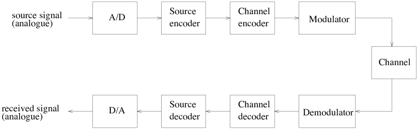
Figure 2.3.1: Conventional stages of a digital communication system

2.3.1 A/D and D/A converters

At the input, an analogue message will be converted into a digital form as binary digits (or bits). Such a conversion is implemented by the so-called Analogue-to-Digital (A/D) converter. At the output, the Digital-to-Analogue (D/A) converter is in charge of reverse process, which converts digital signal back to continuous form. In practice, the A/D and D/A are used in both sampling and quantizing methods upon temporal axis and spatial axis, respectively. Those two methods will be briefly reviewed in this subsection.

2.3.1.1 Temporal sampling

The most important criterion in sampling process is invertible mapping, which guarantees perfect reconstruction of original signal at the output. A sufficient condition for successfully reconstructing signal from its samples is that the sampling frequency at A/D is kept higher than Nyquist rate (i.e. twice the highest frequency) of analogue message, as firstly introduced in [Nyquist (1928)] and later proved in [Shannon (1949)]. Note that, the Shannon-Nyquist sampling theorem is, however, not a necessary condition [Landau (1967)]. Because non-aliased sampled signal in frequency domain is a sequence of shifted replicas of original signal, the reconstruction at D/A is simply an ideal low-pass filter, which crops original signal out of replicas. In time domain, such an ideal filter is called sync filter, which is often replaced by pole-zero low-pass (smoothing) filters like Butterworth or Chebyshev filters [Haykin and Moher (2006)].

Since 1990s, the compressed sensing (CS) technique (also called compressive sampling) has been proposed for sampling sparse signal [Goyal et al. (2008)]. Exploiting the sparsity, compressed sensing projects message signal from original space into much smaller subspace spanned by general waveforms (instead of sinusoidal waveforms in classical technique), while exact recovery is still guaranteed under some conditions [Donoho (2006)]. Nevertheless, a drawback of CS is that the reconstruction has to rely on global convex optimization via linear programming (LP) [Goyal et al. (2008)], instead of deterministic solution like traditional filters. In practice, this technique has been applied to sub-Nyquist rate of multi-band analogue signal [Mishali and Eldar (2009); Tropp et al. (2010)].

2.3.1.2 Spatial quantization

In typical quantization, there are three issues to be considered: vertices of quantized cells, the quantized level within each cell and the binary codeword associated with each level. The first two issues, which are relevant to quantization’s performance, will be reviewed here, while the third issue, which is relevant to practical compression rate, will be mentioned in next subsection on source encoder.

The simplest technique in quantization is to truncate and round analogue value to the nearest boundary in a (either uniform or non-uniform) grid of cells of amplitude axis [Proakis and Manolakis (2006)]. Each quantized level (i.e. the nearest boundary value in this case) will then be assigned by a specific block of bits, which is often called a codeword or symbol. For multi-dimensional case, each dimension of analogue signal can be quantized separately. Such a technique is commonly called scalar quantization in the literature (e.g. [Gersho and Gray (1992)]). In some cases, a transform coding, in which a linear transformation is applied to message signal before implementing scalar quantization, as firstly introduced in [Kramer and Mathews (1956)], might yield better performance than direct scalar quantization, e.g. [Huang and Schultheiss (1963)].

If we regard data as a vector in multi-dimensional space, the vector quantization (VQ) can be used as generalization of scalar quantization (see e.g. [Lookabaugh and Gray (1989)] for their comparison). Instead of using parallel cells in scalar version, VQ divides data space into multiple polytopes pointed to by boundary vectors. Then, VQ maps each message vector within polytope cell into a quantized vector (often being the nearest boundary vector) within that polytope. The virtue of VQ is that any (either linear or non-linear) quantization mapping can be represented equivalently as a specific VQ mapping [Gersho and Gray (1992)]. Hence, VQ is definitely among the best quantization mappings that we can design. In history, original idea of VQ was scattered in the literature. For example, VQ was firstly studied for asymptotic behaviour of random signal in [Zador (1963)], although a version of VQ was used earlier in speech coding [Dudley (1958)]. In computer science, VQ is also known as k-means method, which is named after [MacQueen (1967)] and regarded as cluster classification or pattern recognition method [Jegou et al. (2011)].

Different from sampling, quantization is an irreversible mapping. Hence, the state-of-the-art reconstruction in D/A converter is simply sample-and-holding (S/H) or higher-ordered interpolation operator [Proakis and Manolakis (2006)].

2.3.2 Source encoder and decoder

The purpose of source encoder/decoder is to provide a compromise between compression rate (i.e. number of representative bits per signal symbol) and distortion measure (i.e. error quantity between reconstructed and original signals). Given one of them, the ideal criterion is to minimize the other.

In history, the purely theoretical concept for compression rate was Kolmogorov complexity [Solomonoff (1964); Kolmogorov (1965); Chaitin (1969)], which can be regarded as the smallest number of bits representing the whole data. Because of analysis difficulty, Kolmogorov complexity was subsequently replaced by minimum length description (MDL) principle [Rissanen (1978)], in which the criterion was shifted from finding shortest representative bit-block length to finding an approximate model such that: the total number of bits representing both approximate model and the original signal described by that model is minimal. However, the computation for MDL is still complicated and a subject for current researches [Grunwald et al. (2005)].

The historical breakthrough was a relaxation form of MDL in asymptotic sense, which is the asymptotic bound of rate-distortion function, firstly introduced and proved in foundational papers [Shannon (1948)] and [Shannon (1959)], respectively. On one extreme of this bound, where desired rate is as small as null, we achieve the best compression, but distortion would be high. On other extreme where desired distortion is null, we achieve the so-called lossless data compression scenario, but minimized compression rate is still modest. Compromising those two cases, the lossy data compression scenario, whose purpose is to reduce compression rate significantly within tolerated small loss of distortion, has been widely studied in the literature, as briefly reviewed below.

2.3.2.1 Lossy data compression

This scenario is sometimes called fixed-length code in the literature. Given a fixed compression rate, its popular criterion is to minimize the distortion measure (often chosen as mean square error (MSE)). The research on lossy compression is vast, but currently it can be roughly divided into three domains: A/D converter, transform coding and wavelet-based compression. Note that their separation border might be vague, e.g. Compressed sensing (CS) can be regarded as a hybrid method of the first two methodologies.

In information theory, the A/D converter can be regarded as special case of lossy data compression (e.g. [Goyal et al. (2008); Duhamel and Kieffer (2009)]):

• For a fast sampling scenario, CS has been applied to speed-up medical imaging acquisition [Vasanawala et al. (2010)] or compressive sensor network [Haupt et al. (2008)] with acceptable loss from sparsity recovery. Hence, CS is very useful in the context of expensive sampling, although its compression performance is quite modest [Goyal et al. (2008)].

• In quantization, the Lloyd-Max algorithm [J.Max (1960); Lloyd (1982)] and its generalization Linde-Buzo-Gray algorithm [Linde et al. (1980)] (also known as k-means algorithm) are well-known algorithms for scalar and vector quantization, respectively. Given initial quantized vectors (or quantized levels in scalar case), the k-means algorithm iteratively computes and assigns quantized vector as centroid of probability density function (pdf) of the source signal within quantized cells [Sayood (2006)]. At the convergence, the algorithm returns both boundary values of the cells and quantized levels such that MSE is locally minimized [Sayood (2006)]. In the case of discrete source, if probability mass function (pmf) of the source is unknown, it can be approximated by clusters of input source signal vectors (i.e. similarly to histogram in scalar case) in offline basis, or by adaptive algorithms [Panchanathan and Goldberg (1991)] in online basis.

• Another quantization technique resembling Vector Quantization (VQ) is Trellis Coded Quantization (TCQ), introduced in [Marcellin and Fischer (1990)]. The main purpose of TCQ is to minimize the MSE of entire sequence of quantized source samples, instead of individual MSE of each quantized source sample. In order to avoid the exponential cardinality of trajectory of quantized levels for entire source sequence, TCQ imposes Markovianity—local dependence structure—on those trajectories (i.e. the quantized levels of current source sample will depend on quantized values of previous source sample) [Sayood (2006)]. Then, the trajectory that minimizes MSE can be found via recursive Viterbi algorithm for trellis diagram [Forney (1973)]. In practice, this TCQ scheme was used in standard image compression JPEG 2000 part II [Marcellina et al. (2002)].

Before applying A/D converter, a pre-processing step involving transform coding might be preferred in order to exploit both temporal and spatial correlation in source signal. The main idea of transform coding is to project source signal vector onto the basis capturing the most important features [Duhamel and Kieffer (2009)].

• The earliest transform coding is a de-correlation technique, namely Principal Components Analysis (PCA), firstly proposed for discrete and continuous signal in [Hotelling (1933)] and [Karhunen (1947); Loeve (1948)], respectively. The main idea of PCA is to minimize the geometric mean of variance of transformed components [Sayood (2006)] by using eigenvectors of autocorrelation matrix as a transform matrix. Then, only components with largest variances can be retained as important features of source signal.

• The continuous version of PCA, which is also called Karhunen-Loeve Transform (KLT), is the optimal transformation under MSE criterion, yet its computational load is pretty high [Ahmed (1991)].

• Discrete Cosine Transform (DCT), firstly proposed in [Ahmed et al. (1974)], is another transformation method, with similar performance to KLT but much faster in operation [Ahmed (1991)]. In data compression, the DCT also yields much better performance than Discrete Fourier Transform (DFT), particularly for correlated sources like Markov source, since DCT mirrors the windowed signal and avoids the distorted high frequency effect of sharp discontinuities at the edges [Sayood (2006)]. In practice, DCT is widely used in current standard image compressions, e.g. JPEG, and video compressions, e.g MPEG [Sayood (2006)].

Another pre-processing step is the so-called subband coding, which can be generalized to be wavelet-based compression. The main idea of subband coding is to separate source signal into different bands of frequencies via digital filters, before pushing the outputs through downsampling, quantization and encoding steps [Sayood (2006)]. A drawback of traditional subband method is that the Fourier transform is only perfectly local in frequency domain and none in time, i.e. we cannot indicate when a specific frequency occurs. A trivial method to work around this issue is the short temp Fourier transform (STFT), which divides signal into separate block before applying Fourier transform to each block. However, by uncertainty principle, a fixed window in STFT cannot provide the localization in both time and frequency domains. The wavelet method addresses this problem by re-scaling the window such that low frequencies (longer time window) has higher frequency resolution and high frequencies (shorter time window) has higher time resolution. The wavelet kernel can also be designed with various orthogonal waveforms, instead of strictly sinusoidal waveform in Fourier transform. In practice, wavelet-based method is still not a standard compression technique at the moment [Duhamel and Kieffer (2009)], although there were several applications in image compression, e.g. in JPEG2000 standard.

For reconstruction, since both transform coding and wavelet technique are reversible representation of data, the reconstruction in source decoder is straightforward. Note that, in those cases, the lossy term comes from the fact that some information is truncated by nullifying a subset of coefficients, which does not affect the inverse mapping process. For A/D converter, the reconstruction is similar to D/A converter above, although the reconstructed data is merely an approximation of original data in this case.

2.3.2.2 Lossless data compression

In many cases, lossless compression is required; e.g. in text compression, a wrong character in the reconstructed message might lead to a completely wrong meaning for the whole sentence. Since distortion is assumed null, the ultimate aim of lossless compression is to minimize the total number of representative bits of the source message. Hence, in the data compression process, lossless compression is often applied as the last step in order to reduce further the code length. In that case, the input of lossless compression is discrete source and its p.m.f will be used as an approximation of the p.d.f. of the original source.

In practice, a relaxed criterion, which only requires that minimum message length in an average sense be achieved, is widely accepted. For the sake of simple computation in that average criterion, Shannon’s coding theorem further imposes a fairly strict assumption, where the message source is iid. It shows that no lossless code mapping can produce shorter average compression length than its entropy, which is a function of the p.m.f of that iid source [Shannon (1948)]. Following that result, the current three state-of-the-art algorithms, namely Huffman-code, arithmetic code and Lempel-Ziv code, were designed for three practical relaxations of Shannon’s assumption, respectively: iid source with known p.m.f; iid source with unknown p.m.f and correlated source. These are now reviewed next:

• Huffman code [Huffman (1952)]: Given the p.m.f of a discrete iid source, the famous Huffman code is the optimal (and practical) code mapping, which yields the absolute minimal average code length for the given iid source. Huffman’s minimal average length differs from Shannon’s entropy by one compression bit per source sample, since that is the difference between the integer value of minimal length and the continuous values of entropy [Sayood (2006)]. For fast compression, the Huffman code is designed as a prefix code, in which no code word is a prefix to another codeword [Sayood (2006)]. A prefix code, in turn, can be constructed for Huffman code as a binary tree and facilitate the computation. The Huffman decoder is, owing to this binary tree, fast and feasible since it can traverse through the tree in the same manner as Huffman encoder [Sayood (2006)]. In practice, variants of Huffman code have been used in standard image compression, e.g. JPEG [Chen and Pratt (1984); Sayood (2006)].

• Arithmetic code [Rissanen and Langdon (1979)]: The absolute minimal rate of Huffman code can be further reduced by applying Huffman code to joint p.m.f of multiple block iid source symbols, instead of p.m.f of a single symbol [Cover and Thomas (2006)]. However, despite the fast reciprocal rate reduction, the computation of the joint p.m.f grows exponentially with that number of symbols. In order to avoid that computation, the arithmetic code makes use of two key ideas: Firstly, it quantizes joint cumulative distribution function (c.d.f), instead of joint p.m.f. Secondly, those quantized intervals are refined recursively in an online Markovian fashion (i.e the “child” c.m.f sub-interval of current trajectory divides its “parent” c.m.f interval of previous trajectory). Because the range of c.m.f is the unit interval of real axis, this arithmetic code is capable of representing infinite number of trajectories. Each of them can be assigned as a rational number, with possibly long fractional part (hence the name “arithmetic”), within this unit interval. Owing to Markovianity, the arithmetic code is able tractably to produce a good code rate (within two bits of entropy [Cover and Thomas (2006)]), compared to the minimal rate (within one bit of entropy) of Huffman code above. For decoding, the arithmetic coded sequence in binary base needs to be converted back to its original base value. This conversion raises two issues: the decoding complexity and the rounding of converted values. The former can be solved in a similar manner to the arithmetic encoder, owing to the Markovianity. The latter can be solved in two ways: either the length of original sequence is set a priori, or a pilot symbol is included as the end-of-transmission [Sayood (2006)]

• Lempel-Ziv code [Ziv and Lempel (1977, 1978)]: For correlated source symbols from a set of alphabet, there are two key issues to be solved: firstly, the design for codeword corresponding to each alphabet and, secondly, the design for allocation indices of appearance of that alphabet in a source trajectory. For the first issue, a reasonable approach is to find the p.m.f of alphabet and design a codebook based on that p.m.f. For the second issue, the allocation indices need to be feasible to look up. The famous Lempel-Ziv (LZ) codes solved both issues in an adaptive (i.e online) fashion: the alphabet p.m.f is approximated by sequentially counting the frequency of appearance of the alphabet, while allocation indices can be updated by either sliding window approach (LZ77 algorithm [Ziv and Lempel (1977)]), or a tree-structure approach (LZ78 algorithm [Ziv and Lempel (1978)]). The LZ77 algorithm was proved to be asymptotically optimal in [Wyner and Ziv (1994)], by showing that the compression rate of LZ77 converges to entropy for ergodic source [Cover and Thomas (2006)]. Hence LZ77 has been used in many compression standards, e.g. ZIP, and in image compressions, e.g. PNG [Sayood (2006)]. The LZW algorithm, proposed in [Welch (1984)] as a variant of LZ78, is widely used in many compression standards, e.g. GIF [Sayood (2006)], owing to its similar performance to LZ78 and feasible implementation [Duhamel and Kieffer (2009)]. The LZ codes also belong to the class of dictionary code, because of its alphabet-frequency-index (hence the name dictionary) technique. The decoding process for dictionary code is similar to table-lookup process, where the table is the constructed dictionary and the look-up process is implemented via allocation indices sent to the receiver.

In the literature, the types of lossless compression technique can also be divided in several ways, such as: fixed-length-code (e.g Huffman code) versus variable-length-code (e.g. arithmetic and LZ codes), static code (i.e. offline) versus adaptive code (i.e. online), or entropy code (i.e. for a known source p.m.f like Huffman code and arithmetic codes) versus universal code (i.e. for an unknown source p.m.f like arithmetic and LZ codes), etc.

The early history of data compression is interesting and involves the generation of students in the era after Shannon: Shannon and Fano, who were among the first pioneers of information theory, proposed the theoretical Shannon-Fano coding in order to exploit c.d.f of the source [Cover and Thomas (2006)], although it had never been used until arithmetic code was invented. In Fano’s class of information theory at MIT, his two students, Huffman and Peter Elias, also designed two recursive lossless compression techniques, the Huffman and Shannon-Fano-Elias coding, respectively, although the later was never published [Sayood (2006)].

Similarly to data compression, the early history of channel coding, as briefly reviewed below, is just as interesting: Hamming was a colleague of Shannon at Bell Labs when he invented the Hamming code [Hamming (1950)], which was also mentioned in [Shannon (1948)]. Soon after, Peter Elias invented convolutional code [Elias (1955)], which, much later, subsequently led to the invention of the revolutionary Turbo code [Berrou et al. (1993)]. Gallager, a PhD student of Elias, invented another revolutionary code, namely low-density-parity-check (LDPC) code, in his doctoral thesis [Gallager (1962)].

2.3.3 Channel encoder and decoder

When transmitted through a noisy channel, the bit stream can become corrupted and unrecoverable. A reasonable solution is to strengthen the transmitted message by adding in some extra bits, whose purpose is to protect against the noise effect on message bits. Together, the message and extra bits construct the so-called code bits, which are transmitted through the channel. When the original message bits are corrupted, those extra bits will be a valuable reference for the channel decoder at a receiver to recover the message bits (hence the name error-correcting-code in the literature).

Nevertheless, too many extra bits requires too much redundant energy in the transmitter and thereby increases the operational cost of communication devices. The purpose of the channel encoder, therefore, is to maximize the code rate (i.e. the ratio between number of message bits and number of code bits), while maintaining the possibility of acceptable distortion at the receiver. There exists, however, a limit for the code rate. In the foundational paper of information theory [Shannon (1948)], Shannon’s channel capacity theorem introduced the asymptotic upper bound of channel code rate, which is called channel capacity and is solely dependent on the channel characteristics, provided that the asymptotic average distortion is zero. Since then, a lot of effort has been made to design the optimal channel codes, whose code rate is close to that upper bound. Because of analysis difficulty in optimal case, a relaxed criterion, where distortion is not zero but very small, has been widely accepted in practice.

In summary, a good channel code should satisfy three practical requirements: high code rate, low computational load and sufficiently large Hamming distance between any two codewords. The first and second ones represent the requirement of low operational cost and speed of the communication system, respectively. The third one is a consequence of the channel characteristics (e.g. large Hamming or Euclidean distance between codewords would reduce the uncertain error in binary symmetric channel (BSC) and additive white Gaussian noise (AWGN) channel, respectively). In order to facilitate the analysis of this requirement, all linear codes currently make use of a max-min criterion: maximizing the minimum codeword weight (i.e. its Hamming distance to the origin). Because the sum of any two linear codewords in the finite field is also a codeword, that criterion is equivalent to the task of maximizing the minimum distance between any two codewords [Moon (2005)]. At the moment, non-linear channel codes have not been much investigated or applied in practice [Ryan and Lin (2009)]

The first codes satisfying all three requirements are two capacity-approaching codes: LDPC and Turbo codes, which also reflect two main research domains of channel code, namely block code and stream code, respectively. We review this domain next.

2.3.3.1 Block code

A typical block code is a bijective linear mapping from the original message space into a larger space, namely codeword space, over the binary finite field. Owing to the tractability of linearity and the availability of Galois field theory, research over channel codes has been mostly focussed on this algebraic coding type in the early decades, see e.g. [Berlekamp (1968); Peterson and E. J. Weldon (1972)]. Four historical milestones of block code in this period will be briefly reviewed below.

• Hamming code [Hamming (1950)]: The first practical channel code is Hamming code, whose minimum Hamming distance is three. Hence, it is capable of correcting one error bit with a hard-information decoder [Moon (2005)] and it is also called the class of single-error-correcting code [Costello and Forney (2007)]. However, the performance of Hamming is pretty modest in the AWGN channel, even with soft-decoder.

• Reed-Muller code [Muller (1954); Reed (1954)]: Reed-Muller codes were the first codes providing a mechanism to design a code with desired minimum distance [Moon (2005)]. Another attractive property is speed of decoding, which is based on fast Hadamard transform algorithms [Moon (2005)]. Although it was soon replaced by slightly better performance codes (e.g. BCH code), it is still the best binary code for short-length block codes and is currently being revisited in the literature, owing to its good trade-off between performance and complexity via trellis decoder [Costello and Forney (2007)].

• Cyclic codes [Prange (1957)]: In cyclic codes, any cyclic shift of a codeword yields another codeword. Hence, its efficient encoding via cyclic shift-register implementation is of advantage over other block codes. The major class of cyclic codes with large minimum distance is the BCH codes, which was firstly introduced in [Bose and Ray-Chaudhuri (1960); Hocquengbem (1959)]. However, the asymptotic performance of BCH is not good (indeed, when its code length at a fixed code rate becomes longer, the fraction of errors that is possible to correct is close to zero [Moon (2005)]). Eventually BCH was dominated by its non-binary version, namely Reed-Solomon code [Reed and Solomon (1960)]. The ability of correcting burst-error in RS makes it suitable for disk storage systems, and hence, RS was widely used in compact disk (CD) writing system [Costello and Forney (2007)]. The important property of both BCH and RS is that they can be efficiently decoded via finite field arithmetic [Moon (2005); Costello and Forney (2007)].

• LDPC code [Gallager (1962)]: Instead of designing the encoder directly, LDPC code relies on the design of sparsity in the parity-check matrix, which imposes sum-to-zero constraint on multiple linear combinations of codewords. LDPC code had been forgotten for over thirty years, until it was re-discovered in [MacKay and Neal (1995)], which demonstrated the capacity-approaching performance of LDPC code. Indeed, LDPC has excellent minimum distance, which increases with the block code length (i.e. as the parity-check matrix becomes more sparse) [Moon (2005)]. As the code length goes to infinity, LDPC codes have been shown to reach channel capacity [MacKay (1999)]. Owing to much lower error floor than Turbo code, LDPC code has been chosen in many standard communication system, e.g. in DVB-S2 for digital television or satellite communication system in NASA-Goddard Space Flight Center [Chen et al. (2004)]. However, a drawback of LDPC is the complicated encoding. Although the iterative decoding complexity via message-passing algorithm only grows linearly with block code length, owing to the sparsity, its dual encoder complexity grows quadratically in block length. By some pre-processing steps, the LDPC encoding complexity can be reduced significantly, and close to linear in some cases, as proposed in [Richardson and Urbanke (2001)]. Applying finite geometry, a class of quasi-cyclic LDPC codes was recently proposed in order to achieve linear encoding via cyclic shift-registers [Chen et al. (2004); Ryan and Lin (2009)]. Another drawback of LDPC is that its efficient decoding is only an approximation, not an exact arithmetic solution.

Following the success of LDPC code, many researchers have focussed on improving its decoding approximation, rather than designing a new class of block encoder. Nevertheless, block codes have been received more attention recently. Owing to the availability of algebraic methodologies for finite field, the current trend is to design a good performance code with shorter block length [Costello and Forney (2007)], since Shannon’s channel limit is only valid for asymptotic case after all.

2.3.3.2 Stream Code

By general definition, a stream code is a block code with infinite length. In practice, the distinction between block code and stream code is that the latter can continuously operate on a stream of source bits (i.e. online case) and produce the same code bits as if it operates on divided blocks of sources bits (i.e. offline case). The key advantage of stream code is low complexity and delay of encoder. However, its key drawback is the lack of a mathematical framework for evaluating the encoder’s performance. Currently, all good stream codes have to be designed via trial-and-error simulation [Moon (2005); Costello and Forney (2007)]. For a brief review, two state-of-the-art stream codes will be introduced below:

• Convolutional code [Elias (1955)]: The first practical stream code is Convolutional code, which maps source bits to code bits via linear filtering operators (hence the name “convolution”) [Richardson and Urbanke (2008)]. In the encoder, the filtering process is very fast, owing to the deployment of shift-register memory circuits. In decoder, the changing of shift-register value can be represented via the trellis diagram, whose transitions, in turn, can be inferred jointly or sequentially via state-of-the-art Viterbi [Viterbi (1967)] or Bahl-Cocke-Jelinek-Raviv (BCJR) [Bahl et al. (1974)] algorithms, respectively. Owing to Markovianity, the transmitted sequence can be recursively traced back via those inferred transitions, provided that the pilot symbol at the beginning-of-transmission is known a priori.

• Turbo code [Berrou et al. (1993)]: The first practical stream code approaching Shannon limit is Turbo code, which was initially designed as a parallel concatenation of two Convolutional codes connected by a permutation operator. That initial proposal for Turbo code, although designed via trial-and-error process [Berrou (2011)], has revived the study of near-Shannon-limit channel codes and is still the best performing method for the Turbo code class at the moment [Moon (2005)]. For Turbo decoding, the output of the Convolutional decoder in each branch are iteratively fed as input to the other brach until convergence. This iterative decoding (hence the name ’Turbo’ ) is, however, not guaranteed to converge, although empirical studies show that it often converges in practical applications [Moon (2005); Richardson and Urbanke (2008)]. A drawback of Turbo code is that its error-floor of bit-error-rate (BER) is rather high at $10^{-5}$, owing to low minimum codeword distance. For high quality transmission, whose BER requirement is much lower than $10^{-5}$, the LDPC code with BER error-floor around $10^{-10}$ is much preferred [Ryan and Lin (2009)]. Currently, Turbo code is being applied in many standard systems (e.g. CDMA2000, WiMAX IEEE 802.16, etc. [Berrou (2011)]), although telecommunications systems have gradually shifted from Turbo code to LDPC code, owing to LDPC’s good performance, as explained above.

2.3.4 Digital modulator

The primary purpose of the digital modulator is to map a set of bits to a set of sinusoidal bandpass signals for transmission. In the design process of this mapping, there are three practical criteria to be considered: power efficiency, spectral efficiency and bit detection performance. In practice, if one of them is fixed, the other two are reciprocally dependent on one another.

Hence, there exists a natural trade-off in modulation design. Loosely speaking, a modulation scheme is called more power efficient and/or more spectral efficient if it needs less SNR-per-bit $E_{b}/N_{0}$ (also called bit energy per noise density) and/or it can transfer more bit-rate $R$ as a ratio of the ideal channel’s bandwidth $B$ (also called spectral-bit-rate or spectral efficiency $R/B$) , respectively, to achieve the same bit-error-rate (BER) performance. Note that the maximum bit-rate $R$ for reliable transmission is the Shannon channel capacity $C$ while the maximum sampling rate for zero intersymbol interference (ISI) is the Nyquist rate $2B$. The spectral efficiency $R/B$, therefore, reflects the ratio between transmitter’s bit rate and receiver’s sampling rate in a reliable and zero ISI transmission. In the ideal scenario, where BER average is asymptotically zero, the reciprocal dependence between power and spectral efficiency is given by equation (2.1.1), owing to Shannon channel capacity theorem [Ha (2010)].

Despite the similarity in mathematical formulae and performance criteria, the channel encoder and digital modulator are basically different in the choice of the fixed term in three way trade-off above. Indeed, the study of the channel encoder often neglects the spectral efficiency issue, while digital modulation is mostly designed for reliable transmission only (i.e. BER performance is kept fixed and small). Hence, the channel encoder, whose main purpose is to achieve low BER at low SNR, can be regarded as a pre-processing step for digital modulation, which focuses on trade-off between power efficiency and spectral efficiency. This is a reasonable division of tasks, because modulation involves a D/A step and, hence, requires the study of signal spectrum, while encoding only involves digital bits. Nevertheless, the interface between them is, sometimes, not specific [Schulze and Lueders (2005)]. This vague interface also happens between channel decoder and digital demodulator, as we will see in Section 2.3.6.2.

As stated above, the purpose of digital modulation is to map information bits to amplitude and/or frequency and/or phase of a sinusoidal carrier, such that the trade-off between power efficiency and spectral efficiency in a reliable transmission scheme is optimal. The solution for that trade-off can be divided into two modulation schemes: either “memoryless mapping” or “mapping with memory”, i.e. either on a symbol-by-symbol basis or via a Markov chain, respectively [Proakis (2007)].

2.3.4.1 Memoryless modulation

When bandwidth is the premium resource, modulation on the carrier amplitude and/or phase is preferred to carrier frequency. In the memoryless scheme, each block of $k$ bits, called symbol, is separately mapped to $M=2^{k}$ bandpass signals, whose characteristic is represented by constellation points, as follows:

• Binary (bit) modulation: In this case, the carrier’s amplitude, phase or frequency can be modulated via Amplitude, Phase or Frequency Shift Keying, i.e. ASK, PSK and FSK scheme, respectively. Regarding ASK, also called on-off keying (OOK), it is mostly used in fiber optic communication, because it can produce a bias threshold for turning on-off the light-emitting diode (LED) [Chow et al. (2012)]. Regarding PSK, which is perhaps the most popular binary modulation [Ha (2010)], it simply exploits the antipodal points to represent the binary bits. That simple implementation, however, might introduce phase ambiguity at the receiver. Regarding FSK, which is a special and discrete form of Frequency Modulation (FM), the bit is represented by a pair of orthogonal carriers, whose frequencies are integer multiple of the bit rate $1/T_{b}$. That bit rate is also the minimum frequency spacing required for preserving orthogonality [Ha (2010)]. Despite its simplicity, binary modulation has, however, low spectral efficiency.

• $M$-ary modulation: In this case, the spectral efficiency can be greatly improved at the expense of power efficiency. The popular criterion in this case is average Euclidean distance between constellation points and origin, which reflects both error vulnerability and power consumption of a transmitter. Hence, the $M$-ary ASK, which produces $M$-ary pulse amplitude modulation (PAM), uses more power to achieve the same BER performance as ASK, owing to the increase of average Euclidean distance. Inheriting the high spectral efficiency of $M$-ary ASK, the $M$-ary PSK provides higher power efficiency by increasing the symbol’s dimension from a line in $M$-ary ASK to a circle in the Argand plane.
  For large $M$, however, $M$-ary PSK is not power efficient, because the Euclidean distance of adjacent points in the circle of $M$-ary PSK becomes small with increasing $M$. The $M$-ary Quadrature Amplitude Modulation (QAM) resolves this large $M$ issue by placing the constellation points throughout the Argand plane, also known as in-phase and quadrature (I-Q) plane, corresponding to real and imaginary axis in this case. Furthermore, QAM often employs the Gray code, in which two neighbour points differ only by one bit, in order to decrease the uncertainty error between neighbour points. Owing to those two steps, QAM is widely used in high spectral efficiency communication, e.g. in current standard ITU-T G.hn of broadband power-line, wireless IEEE 802.11a.g or WiMAX IEEE 802.16 [Iniewski (2011)].

For further increasing spectral efficiency with small loss of power efficiency, a solution is to introduce orthogonality between carriers. In this way, the correlator at the receiver can recover transmitted information without interference, even when the set of possible carriers is overlapped at the same time and/or frequency (hence the increase in spectral efficiency). Because scaling does not affect the orthogonality [Ha (2010)], the amplitude of orthogonal carriers can be normalized such that the transmitted power average is kept unchanged (hence small loss in power efficiency). In practice, there are two approaches for designing such orthogonality, either via digital coded signals or via analogue multi-carriers, respectively, as reviewed next:

• Code Shift Keying (CSK): The simplest method of orthogonal coded modulation is CSK, which bijectively maps $M$ information symbols to $M$ orthogonal coded signals, notably Walsh functions [Ha (2010)]. In practice, the number of orthogonal coded signal can be limited, given a fixed symbol period. The orthogonal condition of coded streams can be relaxed to a low cross-correlation condition of pseudo-random or pseudo-noise (PN) code streams. Depending on the modulation scheme (PSK or FSK) that the PN code is applied to, the result is called direct sequence (DS) or frequency hopped (FH) spread spectrum signal, respectively [Proakis (2007)]. The name spread spectrum comes from the fact that the rate is higher than unity, i.e. the coded symbol period $T_{c}$ is smaller than the information symbol period $T_{s}$. The signal bandwidth is, therefore, increased from $1/T_{s}$ to $1/T_{c}$ [Schulze and Lueders (2005)].
  In multiple-access communication systems, where multiple users share a single carrier, a similar orthogonal coding scheme is implemented via Code Division Multiplexing (CDM), which multiplexes different user bit streams orthogonally onto one carrier. In broader communication networks, where users share the same channel bandwidth, CDM is generalized to Code Division Multiple Access (CDMA), which is the standard spread spectrum technique in 3G systems [Schulze and Lueders (2005)]. The combination of CSK modulation with CDMA system is also a research topic, aimed at increasing recovery performance and decreasing user data interference [Tsai (2009)].

• Orthogonal Frequency Division Multiplexing (OFDM): OFDM is a key of 4G system, as reviewed in Section 2.1.2.1. The key idea of OFDM is to employ orthogonal sub-carriers, before multiplexing them into a single carrier for transmission. There are, however, two different viewpoints on this concept of multi-carrier modulation [Schulze and Lueders (2005)]: (i) in practical viewpoint, each time slot $T_{s}$ for the symbol period is fixed, while a filter bank for $K$ bandpass filters, whose minimum frequency spacing is symbol rate $1/T_{s}$ to preserve the orthogonality of the sub-carriers, is employed for $K$ symbol pulse shapes of parallel data sub-streams; (ii) In the textbook’s viewpoint, the number $K$ of sub-carrier frequencies is fixed, while modulation (e.g. QAM) is employed for sub-carriers in time direction (hence, OFDM is also called Discrete Multi-Tone (DMT) modulation if QAM is used [Proakis (2007)]). Note that, because a pulse cannot be strictly limited in both time and frequency domains, (i) and (ii) are merely two viewpoints of the same process: either truncating frequency-orthogonal time-limited pulse in frequency domain, or truncating time-orthogonal band-limited pulse in time domain, respectively. The method (i) is preferred in practice, because, owing to the inverse Fast Fourier Transform (FFT), the OFDM is a fast synthesis of Fourier coefficients modulated by data sub-streams. Furthermore, before transmission, the D/A converter for that synthesized digital carrier can be feasibly implemented via oversampling (i.e. padding zero over unused DFT bins) in digital filters, instead of via complicated analogue filters [Schulze and Lueders (2005)].
  Historically, although the original idea of multi-carrier transmission was first proposed in [Chang (1966); Saltzberg (1967)] via a large number of oscillators, the implementation via digital circuits for high-speed transmission was out of question for a long time [Schulze and Lueders (2005)]. By including an extra guard time-interval, which adds a cyclic prefix in the DFT block to itself, OFDM was rendered suitable for mobile channels [Cimini (1985)]. Indeed, the periodic nature of the DFT sequence in guarding-interval makes the start of original symbols always continuous and greatly facilitates the time synchronization issue in mobile systems [Ha (2010)]. Since then, the main motivation of multi-carrier systems is to reduce the effects of intersymbol interference (ISI), although the application is two-fold. One one hand, longer symbol period and, hence, smaller frequency spacing makes the system more robust against channel-time dispersion and channel-spectrum variation within each frequency slot, respectively [Proakis (2007)]. On the other hand, phase and frequency synchronization issues become more severe than in traditional systems. Hence, in practice, OFDM has been used in Wireless IEEE 802.11 and the terrestrial DVB-T standard, while the cable DVB-C and satellite DVB-S systems still employ conventional single carrier modulations [Schulze and Lueders (2005)]. The combination of CDMA and OFDM, namely Multi-carrier CDMA, is also a promising method for future mobile systems [Hanzo (2003); Fazel and Kaiser (2003)].

2.3.4.2 Modulation with memory

When power is the premium resource, modulation of carrier frequency and of phase is preferred to carrier amplitude. Because the signal is often continuously modulated in this case, it introduces a memory (Markov) effect, in which the current $k$ symbol depends on the most recent, say $L$, symbols. Hence, this modulation with memory can be effectively represented via a Markov chain model, as follows:

• Differential encoding: The simplest modulation scheme with memory is differential encoding, in which the transition from one level to another only occurs when a specific symbol is transmitted. That level can be a Markov state of either phase or amplitude, corresponding to differential $M$-ary PSK or Differential QAM [Djordjevic and Vasic (2006)], respectively.

• $M$-ary FSK: In this case, the frequency bandwidth can be divided into $M$ frequency slots, whose minimum frequency spacing is symbol rate $1/T_{s}$ to preserve the orthogonality of $M$ sinusoidal carriers. Different from linear modulation scheme like QAM (i.e. the sum of two QAM signals is another QAM signal), FSK is a non-linear modulation scheme, which is more difficult to demodulate. Another major drawback of $M$-ary FSK is the large spectral side lobes, owing to abrupt switching between $M$ separate oscillators of assigned frequencies [Proakis (2007)]. The solution is to consider a continuous-phase FSK (CP-FSK) signal, which, in turn, modulates the single carrier’s frequency continuously. In general, CP-FSK is a special case of continuous phase modulation (CPM), where the carrier’s time-varying phase is the integral of pulse signals, and represents the accumulation (memory) of all symbols up to the modulated time [Proakis (2007); Ha (2010)]. In the literature, CPM is an important modulation scheme and widely studied because of its efficient use of bandwidth [Rimoldi (1988); Graell i Amat et al. (2009)].

In order to increase power efficiency further with small loss of spectral efficiency, a solution is to design an effective constellation mapping in higher dimensional space. For example, the dimension of a trajectory of $n$ $M$-state symbols is $M^{n}$, which increases exponentially with $n$. Although the constellation design in the I-Q plane can only be applied in two dimensions, its design principle can be applied to a trajectory in $M^{n}$ dimensions. Then, the criterion for the trajectory’s constellation mapping can be chosen as a max-min problem, which is to maximize the minimum Euclidean distance between any two trajectories. Note that, the Gray code mapping for $n$ separate symbols may fail to achieve that criterion and may yield only a small increase in power efficiency [Ha (2010)].

• Trellis Coded Modulation (TCM) [Ungerboeck (1982)]: The power efficiency, also known as coding gain, can be greatly improved via TCM. The trajectory’s constellation in TCM is designed via a principle of mapping by set partitioning, i.e. the minimum Euclidean distance between any two trajectories is increased with any partition of I-Q constellation of each new symbol. Hence, the active point in current I-Q constellation depends on both current symbol and the active point in previous I-Q constellation. In other words, the current symbol does not point to a point in I-Q constellation like in QAM, but to a transition state between two consecutive I-Q constellation planes (hence the name Trellis in TCM) [Proakis (2007)]. In the literature, the TCM is mostly designed to map the channel stream-code bits (e.g. via Convolutional or Turbo code), instead of original bit stream, in order to increase the joint decoder and demodulator performance [Moon (2005)]. There is, however, no mapping guaranteed to achieve optimal Euclidean distance or BER performance [Anderson and Svensson (2003)]. In current standard systems, although TCM is not selected in Wireless IEEE 802.11a [Terry and Heiskala (2002)], owing to difficulty in design, it has been applied in Wireless IEEE 802.11b and IEEE 802.15.3 [Progri (2011)]

2.3.5 The communication channel

The communication channel is, by definition, the physical medium for transmission of information. In practical channels, the common problem is that, owing to unknown characteristics of the channel and transmission devices, random noise will be added to the transmitted signal. These unknown quantities yields an uncertain signal, whose original form can be inferred from the channel’s probability model. Two major concerns in the channel model are transmitted power and available channel bandwidth, which represents the robustness against noise effect and the physical limitations of the medium, respectively. Corresponding to those two concerns, the characteristics of three major models in the literature, namely AWGN, band-limited and fading channels, respectively, will be briefly reviewed below. Those three channels represent the former concern, the latter concern and both of them, respectively.

2.3.5.1 The Additive White Gaussian Noise (AWGN) channel

The simplest model for the communication channel is the additive noise process, which often arises from electronic components, amplifiers and transmission interference. The noise model for the third cause will be discussed in fading channel model below. For the first two causes, the primary type of noise is thermal noise, which can be characterized as Gaussian noise process [Proakis (2007)] (hence the name additive Gaussian channel). The noise is often assumed to be white, that is, it has constant power spectral density (PSD), usually denoted $N_{0}$ or $N_{0}/2$ for one-sided or two-sided PSD, respectively. The Gaussian noise process is, therefore, wide-sense stationary and zero mean. In the literature, the AWGN channel is perhaps the most widely used model, owing to its mathematical simplicity.

Nevertheless, the AWGN model is a mathematical fiction, because its total power (i.e. the PSD integrated over all frequencies) is infinite [Schulze and Lueders (2005)]. Its time sample has infinite average power and, therefore, cannot be sampled directly without a filter. In the literature, the ideal output of that filter at the receiver is a noise model with finite power, namely discrete AWGN, which is an iid Gaussian process with zero mean.

2.3.5.2 Band-limited channel

In some communication channels, the transmitted signals are constrained within a bandwidth limitation in order to avoid interference with one another. If the channel bandwidth $B$ is smaller than the signal bandwidth, the modulated pulse will be distorted in transmission. In theory, the Nyquist criterion for zero intersymbol interference (ISI) provides the necessary and sufficient condition for a pulse shape to be transmitted over flat response channel without ISI. Such a pulse with zero ISI is also called the Nyquist pulse in the literature. The sampling rate $1/T_{s}$ must be greater than or equal to the Nyquist rate $2B$, otherwise the Nyquist pulse does not exist [Ha (2010)]. The Nyquist pulse with minimum bandwidth is the ideal sinc pulse. However, because the sinc pulse is idealized, a raised-cosine filter with small excess bandwidth is often used as Nyquist pulse in practice.

The band-limited channel is also the simplest form of dispersive channel, which responds differently with signal frequency. In practice, a noisy dispersive channel is often modeled as linear filter channel with additive noise. Such a noise can be white or coloured, depending on whether the channel filter is put before or after the noise. The additive colored noise with filtered PSD, which implies correlation between samples, is more complicated and, therefore, is typically transformed back to white noise model via a whitening filter at the receiver.

2.3.5.3 Fading channel

In the mobile system, the transmitted signal always arrives at the receivers as a superposition of multiple propagation paths, which generally arise from signal reflection and scattering in the environment. This type of fading channel actually appears in all forms of mobile wireless communication [Ha (2010)]. The fading process is characterized by two main factors, space varying (or frequency selectivity) and/or time varying (or Doppler shift):

• Space varying (or frequency selectivity)

In the literature, this issue is characterized by a correlation frequency $f_{corr}$ (also called coherence bandwidth), which is the inverse of the delay spread $\Delta\tau$ arising from different traveling time of multiple paths. The fading channel with or without ISI is called frequency selective or flat (non-selective) fading channel, respectively. In practice, flat fading can be approximately achieved if the channel bandwidth $B$ satisfies $B\ll f_{corr}$. Since $B$ is of the order of $T_{s}^{-1}$ for a Nyquist basis, such a condition is corresponding to $\Delta\tau\ll T_{s}$, i.e. the time delay is much smaller than symbol period $T_{s}$.

Note that, unlike ISI caused by channel filtering, the ISI in fading channel is caused by random arrival time of multi-path signal copies and, therefore, cannot be eliminated by pulse shaping in Nyquist criterion for zero ISI [Ha (2010)]. For example, a symbol period $T_{s}=10\ \mu s$, leading to an approximate data rate of $200\ kbits/s$ for QPSK modulation, has the same order as $\Delta\tau=10\ \mu s$ of delay time corresponding to $3\ km$ difference of traveling paths at light speed $c$ [Schulze and Lueders (2005)]. It means that such a data transmission in practice cannot be free of ISI without sophisticated techniques like equalizers, spread spectrum or multi-carrier modulation. For example, the main motivation of OFDM is, intuitively, to prolong the symbol period and, in turn, narrow the signal bandwidth. In this way, OFDM avoids the use of a complex equalizer in demodulation, although the Doppler spreading effect, as reviewed below, destroys the orthogonality of OFDM sub-carriers and results in intercarrier interference (ICI) [Proakis (2007)].

• Time varying (or Doppler shift)

In the literature, this issue is characterized by correlation time $t_{corr}$ (also called variation’s timescale), which is the inverse of maximum Doppler shift $f_{D}=\frac{v}{c}f_{c}$ , given relative speed $v$ between transmitter and receiver and carrier frequency $f_{c}$. For example, the amplitude might be faded up to $-40\ dB$ at Doppler shift $f_{D}=50\ Hz$, corresponding to vehicle speed $v=60\ km/h$ and frequency carrier $f_{c}=900\ MHz$ [Schulze and Lueders (2005)]. The fading channel is called slow or fast fading if signal envelope fluctuates little or substantially within symbol period $T_{s}$, respectively. The condition for slow fading is $T_{s}\ll t_{corr}$, or equivalently $f_{D}T_{s}\ll 1$ (hence the name normalized Doppler frequency $f_{D}T_{s}$). In practice, the fluctuation in carrier amplitude and phase is the superposition of multiple Doppler shifts corresponding to multiple paths, which results in the so-called Doppler spectrum instead of Doppler sharp spectral line at $f_{D}$.

In a probability modelling context, each propagation path is considered to contribute random delay and attenuation to the received signal, whose envelope can be described as Rayleigh fading process (no guided line-of-sight path), or Rician fading process (one strong line-of-sight path), or the most general model, Nakagami fading process. Out of the three, Clarke’s Rayleigh model [Clarke (1968)] is the most widely used model for wide-sense stationary fading process, owing to its mathematical simplicity and tractability, compared to the other two general models for real channel [Proakis (2007)]. Because the power spectral density (PSD) in flat fading with Clarke’s model is not a rational function, such a random process cannot be represented by an auto-regressive (AR) model. This drawback leads to difficulty in evaluation of channel detection [Sadeghi et al. (2008)] and channel simulation [Xiao et al. (2006)].

For feasible evaluation of channel’s detection, the finite-state Markov channel (FSMC) was revived in [Wang and Moayeri (1995)] for modeling the fading channel, owing to its computational simplicity. Since then, the first-order FSMC model has been a model of choice for fading channel, although it is more accurate for slow fading rates than fast fading rates [Sadeghi et al. (2008)].

For feasible simulation, an approximate AR model, with sufficiently large order $M$, for Clarke’s model was proposed in [Baddour and Beaulieu (2005)]. Because such an AR model is essentially a Markov process with order $M$, a high-order FSMC is also more accurate for fast fading channel [Sadeghi and Rapajic (2005)].

2.3.6 Digital demodulator

The purpose of the digital demodulator at receiver is to recover the transmitted symbols carried on the modulated signal. The demodulation is, therefore, an inference task based on the designed modulation scheme and the noise model of the channel. In the practical system, digital demodulation involves two steps, namely a signal processor and digital detector [Ha (2010)]. The former, which can be interpreted as the general form of A/D converter, is to convert the noisy signal into a digital observation sequence, such that sufficient statistics for transmitted symbols is preserved. The latter is to infer transmitted symbols from this converted digital sequence. Those two steps can be implemented sequentially or iteratively, as reviewed below.

2.3.6.1 Signal processor

If the digital detector process is implemented directly in digital software, high sampling rate around carrier frequency would be required. To avoid such over-sampling, the solution is to obtain the lowpass equivalent signal and produce a digital sequence from this lowpass signal. For this purpose, the most important signal processor is the matched filter [Proakis (2007)]. Owing to equivalence between convolution and correlation operator at sampling time point, the matched filter is also equivalent to a correlator, whose purpose is to extract the transmitted symbol via correlation between reference and received signal. For a noiseless channel, this is obviously a perfect extraction. For an additive noisy channel, the matched filter, which is linear, can preserve the additivity of noise model in digital sequence and, therefore, provide sufficient statistics for inferring transmitted symbols.

Nevertheless, there are two major difficulties for the matched filter. Firstly, traditional matched filter requires a coherent demodulation, which assumes that local reference carrier can be synchronized perfectly with received signal in frequency and phase. Secondly, in the band-limited channel, a cascade of a matched filter and an equalizer, which is the compensator for reducing intersymbol interference (ISI), is no longer a matched filter and might destroy the optimality of the original matched filter [Ha (2010)]. Those two issues are also major concern for signal processor in practical system.

• Synchronization

At the receiver, three main parameters, which need to be synchronized between the transmitted and received signal, are carrier phase, carrier frequency and symbol timing. In practice, the state-of-the-art estimation method for those three issues is Maximum Likelihood (ML), although Bayesian techniques for synchronization have been proposed recently in the literature, as reviewed below.

For phase synchronization, the ML phase estimator $\widehat{\phi}_{ML}$ is typically tracked by a Phase-Locked-Loop (PLL) circuit in practice. Instead of computing $\widehat{\phi}_{ML}$ directly, which would require a long observed time and cause delay in computation, the PLL continuously tunes reference phase $\widehat{\phi}$ via a feedback circuit until the value of the likelihood’s derivative against carrier phase becomes zero [Proakis (2007)]. Owing to its adaptability to the channel’s variation and non-data-aided (NDA) scheme, PLL research is extensive in the literature (see e.g. [Lindsey (1972),Bregni (2002)]). Nevertheless, the data-aided (DA) (either pilot-based or non-pilot-based) scheme for phase synchronization significantly increases the accuracy. For pilot-based scheme, ML estimation $\widehat{\phi}_{ML}$ can be derived feasibly [Meyr et al. (1997)]. For non-pilot-based scheme, the estimation accuracy for low SNR is only acceptable via channel code-aided (CA) scheme, although it is only possible to return a local ML phase estimator via iterative EM algorithm in this case [Herzet et al. (2007)]. Recently, in [Quinn et al. (2011)], a Bayesian technique was applied to phase inference in a simple single-tone carrier model, and showing that the Von Mises distribution is a suitable conjugate prior for phase uncertainty in this case.

For frequency synchronization, three state-of-the-art methods in the literature are the periodogram, phase increment and auto-correlation methods [Palmer (2009)]. The periodogram method is equivalent to the ML estimation method [Rife and Boorstyn (1974)], while the other two are low-complexity sub-optimal methods, which exploit the rotational invariance of displaced cisoidal signals [Proakis and Manolakis (2006)]. The technical details of these three methods will be presented in Section 3.2. In practice, the accuracy of frequency estimation is high and, hence, frequency synchronization is much less severe than phase synchronization. For example, in the AWGN channel, the frequency-offset error in OFDM is typically around $1\%$ of the sub-carrier spacing in high SNR [Ha (2010)]. Nevertheless, frequency synchronization for OFDM is more severe in practical channels, e.g. low SNR or fading channel [Schulze and Lueders (2005); Proakis (2007)], because the error in frequency estimation will destroy orthogonality between sub-carriers. Recently, in [Morelli and Lin (2013)], the ESPRIT method was proposed for estimating OFDM’s frequency offset in low-cost direct-conversion receiver (DCR), which demodulates the received signal in analogue domain and, hence, is prone to frequency-selective I-Q imbalance. Regarding Bayesian techniques, the posterior distribution for uncertain frequency is typically not in closed-form because sinusoidal signal is a non-linear model of frequency. Hence, Bayesian techniques for frequency have not been applied in practice, although, recently, the MCMC method was proposed in the literature [Bromberg and Progri (2005)] for approximating the frequency posterior distribution.

For symbol timing, the typical scenario is data-aided (DA) synchronization [Bergmans (1995)]. Such a scheme is reasonable, since symbol timing involves the symbol data to begin with. For the DA scheme, the ML delay estimator can be tracked via delay-locked loop (DLL) circuit, which operates similarly to the PLL for phase. Note that, a variant of DLL, namely Early-gate DLL, can also be applied to non-data-aided (NDA) or low SNR scheme, by marginalizing out assumed equi-probable symbols from observation model [Proakis (2007)]. Carrier phase and symbol timing can also be estimated jointly via joint ML estimator in order to achieve higher accuracy [Falconer and Salz (1977)]. Similarly, the delay time can be estimated along with phase offset in above CA synchronization [Herzet et al. (2007)]. In OFDM, the symbol timing issue is less severe, owing to cyclic prefix of symbols in guard time period [Schulze and Lueders (2005)].

• Equalization

If $H(f)$ is the product of the transmission filter and known channel response, the matched filter $H^{*}(f)$ for zero ISI at receiver can be designed such that the folded spectrum $X(f)$, i.e. the new channel spectrum $H(f)H^{*}(f)$, satisfies the Nyquist criterion for zero interference. Since the channel response is typically unknown, a block of digital equalization filter for reducing ISI usually consists of two parts. In the first part, a digital noise-whitening filter $H_{w}(z)$ is designed such that the colored noise, i.e. the channel’s white noise filtered by matched filter, can be whitened and, hence, uncorrelated. In the second part, a linear digital equalizer, $G(z)$, can be chosen as one of two popular models, namely zero-forcing equalizer $(H(z)H_{w}(z))^{-1}$ (for ideally noiseless channel) and MMSE equalizer (for unknown noisy channel, but with WSS symbol sequence). The former filter forces ISI to zero, but tends to increase noise power and, hence, reduce SNR [Ha (2010)]. The latter filter, whose coefficients can be estimated via the LMS or RLS algorithm, minimizes the mean square error (MSE) between randomly WSS symbol sequence and the output of equalizer [Proakis (2007)]. The performance of linear filter can be significantly increased via the data-aided scheme, also known as the decision-feedback scheme, when combined with digital detector. These decision-feedback equalizers (DFE) are, however, non-linear filters [Ha (2010)]. Note that, since the channel response is not known in practice, adaptive algorithms need to be applied to these equalizers in order to track channel’s characteristics [Proakis (2007)].

2.3.6.2 Digital detector

As mentioned earlier in Section 2.3.4, the interface between the channel decoder and digital detector is blurred. In traditional definition, however, the output of digital detector and, hence, of digital demodulator is hard-information of transmitted symbol sequence, while the channel decoder increases the detector’s performance further, owing to channel encoding methods [Madhow (2008)]. In the literature, the term “demodulation” generally focuses on the output of the digital detector, which relies on modulation scheme and channel characteristics, while the term “decoder” implies the channel decoder, which relies on encoding model (see e.g. [Chen et al. (2003)]).

The state-of-the-art techniques for digital detector are, therefore, ML estimator and ML sequence estimator (MLSE), corresponding to two detector schemes, namely symbol-by-symbol and joint symbol sequence, respectively. Note that, for simplicity in study of demodulation, the bit sequence at the input of modulator is often assumed as an iid Bernoulli uniform sequence. Although ML and MAP estimators are equivalent in this case, the term MAP estimators are often preserved for more complicated input, e.g. Markov source or channel encoding sequence.

• Symbol-by-symbol detector

In this scheme, each transmitted symbol is detected independently from each other. This simple scheme is mostly applied to memoryless modulation with AWGN channel. For the case of $M$-ary modulation, the ML estimator simply returns the constellation point closest in Euclidean distance to observed symbol in constellation plane. For the case of orthogonal modulation, the user streams (in CDMA) and sub-carriers (OFDM) are well separated via correlation in the signal processor above [Schulze and Lueders (2005)]. Hence, the detector for each user stream or sub-carrier is similar to $M$-ary case.

• Symbol sequence detector

In this scheme, transmitted symbol sequence is detected jointly via Markovian model. Given transition values in trellis diagram, the MLSE can be found efficiently via Viterbi algorithm (VA). This powerful scheme has been applied to all kind of modulation and channel models.

For memoryless modulation, the MLSE is applied when ISI occurs and/or symbol timing is difficult. Firstly, $K$ observation samples per overlapped time period will be collected into a sequence of length, say $n$, of $M^{K}$-ary symbols. Secondly, assuming that two consecutive $M^{K}$-ary symbols overlap in $L$ symbols, an $M^{m}\times M^{m}$ augmented transition matrix with $M^{2m}$ valid transitions can be constructed, where $m=2K-L$. Thirdly, the soft-information for each state in $M^{m}$ states are computed from the observation sequence. Finally, the MLSE for those $n$ symbols are returned by VA. For high $n$, such a MLSE is the closest point to the observation sequence in exponentially $O(M^{nm})$-ary constellation plane, while VA’s computational load $O(nM^{2m})$ is always linear with $n$.

Hence, the performance of MLSE is significantly better than that of both symbol-by-symbol detector in AWGN channel and equalizer method in band-limited channel, with modest increase in computational complexity [Proakis (2007)]. A similar result is also achieved in the modulation with memory effect and FSMC-fading channel, since both of them are Markovian model to begin with.

2.4 Summary

In this chapter, we asserted that the challenge for mobile systems is more about efficient computation than performance breakthroughs, as we put this insight into the context of the generational evolution of telecommunications systems. An interesting remark is that the standard transmission speed of any mobile generation, from 1G to 5G, was always set equal to that of fixed-line communication in the previous generation. This insight in the mobile generations illustrates the need for efficient computation and will be used in discussion of future work in Section 9.1.

The fading channel, i.e. the environment that all mobile phones must confront, was also picked out as the main cause of performance degradation. This review also raises the need for better trade-off schemes - between accuracy and speed - for symbol detection in the receiver. For this reason, the fading channel and the search for new trade-offs will receive more attention in this thesis (e.g. sections 3.3 and 8.2, respectively).

To motivate Bayesian inference in this thesis, non-Bayesian techniques were first reviewed, along with their drawbacks. The Least Squares (LS), optimal MMSE estimator, Wiener filter and ML estimator are central techniques in non-probabilistic estimation. Some major limitations in DSP for frequentist techniques, e.g. unbiased estimator, and Bayesian theory, e.g. subjectivity of the prior model, were explained and clarified. The Bayesian methodology introduced in this chapter will be presented in more detail in Chapter 4.

All major operational blocks in the telecommunications system were briefly reviewed in order to emphasize the significant role of Markovianity. Indeed, Markovianity appears in every block of telecommunications system and, more importantly, in most computationally-efficient schemes for these blocks. By Markovianity, we mean the invariant of the neighbourhood structure in each objective functional factor. The distributive law for ring theory will be used in Chapter 5 as an attempt to exploit further the advantage of this Markovianity, which is also one of the main themes for our future work (Section 9.1).

Chapter 3 Observation models for the digital receiver

In this chapter, the demodulation task for three communication scenarios will be briefly reviewed. For simplicity, the channel noise will be assumed to be additive white Gaussian noise (AWGN). As explained in Section 2.3.5.1, despite being idealistic, AWGN model is a major type of corruption, which serves as basic assumption in many practical channels [Proakis (2007)]. In this thesis, let us assume further that there is no intersymbol interference (ISI) and channel time-delay.

As explained in Section 2.2.4.1, analogue form of the received signal can be represented via the Wold decomposition as follows:

$$x(t)=Re\left\{g\left(t\right)\sum_{i=1}^{n}s_{i}u\left(t-iT_{s}\right)\right\}+w(t)$$ (3.0.1)

where $w(t)$ is AWGN process with PSD $\sigma^{2}=N_{0}/2$ (W/Hz), $s_{i}\in\mathcal{A}_{M}$ is the $i$th complex symbol belonging to $M$-ary alphabet $\mathcal{A}_{M}\triangleq\left\{\xi_{1},\ldots,\xi_{M}\right\}$, the wave form $g(t)$ represents both carrier and channel characteristics, $u(t)$ is unit-energy Nyquist pulse shape of duration $T_{s}$.

Let us recall that the case of non-zero ISI can be arranged to be close to zero via equalization, as explained in Section 2.3.6.1. Hence, for simplicity, the case of zero ISI will be assumed in this thesis. Also, as reviewed in the same section, the symbol timing can be synchronized jointly with carrier phase offset. Because the phase synchronization issue will be left for future work, let us assume that the symbol timing can be synchronized perfectly, and that the duration $T_{s}$ is the same for both symbol period and sampling period in this thesis.

Note that, the parameterization $\theta$ of probabilistic observation model $f(x(t)|\theta,\mathcal{I})$ depends on design of model $\mathcal{I}$, which, in turn, depends on characteristics of both carrier signal over channel $g\left(t\right)$ and the source $\mathbf{s}_{n}\triangleq\{s{}_{1},s{}_{2},\ldots,s_{n}\}$. Then, four possible scenarios of model $\mathcal{I}$ are:

• $\mathcal{I}_{1}$ - both known $\{g\left(t\right),\mathbf{s}_{n}\}$

• $\mathcal{I}_{2}$ - known $g\left(t\right)$, unknown $\mathbf{s}_{n}$

• $\mathcal{I}_{3}$ - unknown $g\left(t\right)$, known $\mathbf{s}_{n}$

• $\mathcal{I}_{4}$ - both unknown $\{g\left(t\right),\mathbf{s}_{n}\}$

Leaving out the trivial case $\mathcal{I}_{1}$, three remaining scenarios will be studied in this thesis. More specifically, three basic problems in communication will be considered respectively:

• $\mathcal{I}_{2}$: synchronized symbol detection in AWGN channel (i.e. known carrier and channel characteristics, but unknown symbols)

• $\mathcal{I}_{3}$: pilot-based frequency offset estimation in AWGN channel (i.e. unknown carrier characteristic, but known channel characteristic and symbols)

• $\mathcal{I}_{4}$: synchronized symbol detection in quantized fading channel (i.e. unknown channel characteristic and symbols, but known carrier characteristic)

Those three problems, in respective order, will be presented in three sections below.

3.1 Symbol detection in the AWGN channel

As reviewed in Section 2.3.4, the simplest carrier wave form $\psi(t)$ in this case is a complex sinusoid, as follows:

$$g\left(t\right)=\psi(t)\triangleq ae^{j2\pi f_{c}t}$$ (3.1.1)

where carrier parameters $\theta=\{a,f_{c}\}$, i.e. amplitude $a$ and carrier frequency $f_{c}$, are assumed known in this section. For simplicity, the carrier phase is assumed to be null.

Since $\theta$ is given, the baseband signal can be retrieved and sampled from $x(t)$ via matched filter, designed at carrier frequency. As explained in Section 2.3.6.1, the matched filter is also equivalent to a correlator, owing to duality between convolution and correlation operators. Note that, this equivalence is only valid at sampling point $t=iT_{s}$, $i\in\{1,2,\ldots,n\}$ [Ha (2010)], i.e. we have $x_{I}(iT_{s})=\tilde{x}_{I}(iT_{s})$ and $x_{Q}(iT_{s})=\tilde{x}_{Q}(iT_{s})$ in Fig. 3.1.1. As explained in Section 2.3.6, the correlator is also a general form of A/D converter. The key difference is that the sample in the output of correlator is the result of a projection, instead of sampling values in traditional A/D. Hence, the correlator form will be presented below for the sake of clarity and intuition.

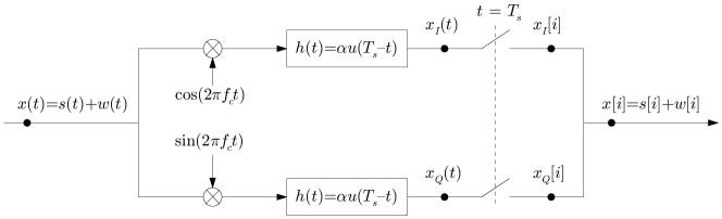
(a)

  

(b)

Figure 3.1.1: The equivalence between matched filter (a) and correlator (b) in quadrature demodulator

In order to exploit the AWGN assumption, the key idea is to construct an orthonormal basis spanning signal space, since the projection of AWGN process in Hilbert space ${\cal H}$ onto that orthonormal basis yields another AWGN process in sub-Hilbert space ${\cal S}$ with the same PSD as the AWGN in ${\cal H}$ [Madhow (2008)]. For this purpose, let us consider a normalization constant $\alpha$ such that the in-phase $\varphi_{I}(t)=\alpha u(t)\cos(2\pi f_{c}t)$ and quadrature $\varphi_{Q}(t)=\alpha u(t)\sin(2\pi f_{c}t)$ components are orthonormal basis functions of signal space. Then, the projections of $x(t)$ and $w(t)$ onto this signal space can be collected as discrete complex variables, as follows:

$$\begin{cases}x_{i}&=\left\langle x(t),\varphi_{I}(t)\right\rangle+j\left\langle x(t),\varphi_{Q}(t)\right\rangle\\ w_{i}&=\left\langle w(t),\varphi_{I}(t)\right\rangle+j\left\langle w(t),\varphi_{Q}(t)\right\rangle\end{cases},\ \frac{t}{T_{s}}\in[i-1,i)$$ (3.1.2)

where $\left\langle\cdot,\cdot\right\rangle$ is the inner product in $i$th symbol interval, $i\in\{1,2,\ldots,n\}$. Hence, the output of quadrature demodulator in this case is the basic discrete complex receiver in AWGN channel [Forney and Ungerboeck (1998)], as follows:

$$x_{i}=s_{i}+w_{i},\ i\in\{1,\ldots,n\}$$ (3.1.3)

where the projection $w_{i}$ of $w(t)$ via (3.1.2) is a discrete complex AWGN sequence, i.e. $w_{i}\sim\mathcal{CN}(0,\sigma^{2})$, with the same variance $\sigma^{2}=N_{0}/2$ as $w(t)$ [Madhow (2008)]. Hence, the observation model can be written as follows:

$$f(x_{i}|s_{i})=\mathcal{CN}_{x_{i}}(s_{i},\sigma^{2}),\ i\in\{1,\ldots,n\}$$ (3.1.4)

In classical estimation, the Maximum Likelihood (ML) estimator for Gaussian noise can be found via the Least Squares (LS) method. In the simplest case where $\mathbf{s}_{n}$ is a uniform iid sequence, each symbol can be estimated separately, i.e. $\widehat{s_{i}}=\arg\min_{s_{i}\in\mathcal{A}_{M}}\left\|x_{i}-s_{i}\right\|^{2}$, $i\in\{1,2,\ldots,n\}$ . For more general case where $\mathbf{s}_{n}$ is a Markov source, Bayesian inference is needed. This Markovian case will be studied in Chapter 8.

3.2 Frequency estimation in the AWGN channel

When carrier parameters $\theta=\{a,f_{c}\}$ are unknown, e.g. owing to offset corruption in channel, a common solution for these time-invariant parameters is to transmit a block of $n$ known symbols (also called pilot symbols), in order to estimate $\theta$ before estimating true messages coming afterward [Ha (2010)]. Hence, without loss of generality, let us assume that $s_{i}=1$ for all $i\in\{1,2,\ldots,n\}.$ The carrier frequency $f_{c}$ in this case becomes $f_{c}+\Delta f$, where $\Delta f$ is the unknown offset frequency. Denoting $f_{s}\triangleq 1/T_{s}$ as symbol rate and $f_{o}\triangleq T_{s}\Delta f=\frac{\Delta f}{f_{s}}\in[-0.5,0.5)$ as normalized offset frequency, the channel wave form $g\left(t\right)$ in (3.1.1) now becomes:

$$g\left(t\right) = ae^{j2\pi(f_{c}+\Delta f)t}$$

$$= \psi(t)e^{j2\pi\Delta ft}$$

$$\approx \psi(t)e^{j2\pi if_{o}},\ \frac{t}{T_{s}}\in[i-1,i)$$

in which the approximation in (3.2) is valid if $\Delta f$ is sufficiently smaller than symbol rate $f_{s}$, or equivalently $f_{o}\ll 1$. If this assumption is valid, receiver can feasibly operate in steady-state condition, i.e. symbol timing is synchronized first before $f_{o}$ is estimated [Mengali and D’Andrea (1997)]. Applying the matched filter (i.e. correlator) at nominal carrier frequency $f_{c}$ like above, the discrete complex data (3.1.3) now becomes:

$$x_{i} = ae^{j2\pi if_{o}}+w_{i}$$

$$= ae^{j\Omega_{o}i}+w_{i},\ i\in\{1,\ldots,n\}$$

where $w_{i}$ is discrete AWGN sequence with variance $\sigma^{2}=N_{0}/2$ and $\Omega_{o}$ is digital offset frequency, with $\Omega_{o}\triangleq 2\pi f_{o}\in[-\pi,\pi)$. The observation model can be written as follows:

$$f(x_{i}|a,\Omega_{o})=\mathcal{CN}_{x_{i}}(ae^{j\Omega_{o}i},\sigma^{2}),\ i\in\{1,\ldots,n\}$$ (3.2.3)

In the literature, the common concern is to estimate $\Omega_{o}$, while amplitude $a$ is regarded as a nuisance parameter. Despite being classical, single frequency estimation is still an interesting issue in practice, as revised by [Klein (2006); Morelli and Lin (2013)]. The important challenge is a trade-off between computational complexity and estimation performance, particularly in the case of low signal-to-noise ratio ($SNR$) [Klein (2006)]. For this issue, the periodogram, phase increment and auto-correlation are currently three most common techniques in practice [Palmer (2009)] and will be briefly reviewed below.

3.2.1 Single frequency estimation via Periodogram

For a batch of data $\mathbf{x}_{n}$, the classical Maximum Likelihood (ML) estimator for frequency $\Omega_{o}$ is equivalent to the maximum of periodogram [Rife and Boorstyn (1974)]:

$$\widehat{\Omega_{o}}=\arg\max_{\Omega_{o}}\left|\sum_{i=1}^{n}x_{i}e^{-j\Omega_{o}(i-1)}\right|^{2}$$ (3.2.4)

In practice, the value of periodogram at DFT bins $\Omega_{o}=\frac{2\pi}{n}m$ with $m\in\{0,\ldots,n-1\}$ can be computed via Discrete Fourier Transform (DFT) [Palmer (2009)]. When $SNR=a^{2}/2\sigma^{2}$ is sufficiently high, the Mean Square Error (MSE) of ML estimator $\widehat{\Omega_{o}}$ approaches the Cramér-Rao bound (CRB) for frequency estimators [Rife and Boorstyn (1974)]. However, when $SNR$ is below a certain threshold, the MSE of $\widehat{\Omega_{o}}$ rapidly increases [Brown and Wang (2002)]. Another drawback of periodogram is a high computational cost, even with sub-linear complexity $\mathcal{O}(n\log n)$ of FFT algorithm. [Brown and Wang (2002)]. Hence, many sub-optimal estimators have been proposed to reduce the computational complexity [Klein (2006)].

3.2.2 Single frequency estimation via phase increment

In order to avoid the high complexity in non-linear estimator in (3.2.4), the noisy model for $x_{i}$ in (3.2) can be approximated by a noisy linear form when $SNR$ is sufficiently high, as follows [Tretter (1985)]:

$$x_{i}\approx ae^{j\phi_{i}}=ae^{j(\Omega_{o}i+\eta_{i})},\ i\in\{1,\ldots,n\}$$

Hence, the observed data in this case is:

$$\phi_{i}=\Omega_{o}i+\eta_{i},\ i\in\{1,\ldots,n\}$$ (3.2.5)

where $\eta_{i}$ is discrete AWGN sequence with variance $\sigma^{2}/2a^{2}$, i.e. $var(\eta_{i})=0.5/SNR$ [Tretter (1985); Kay (1989)]. In order to avoid phase unwrapping in (3.2.5), Kay’s method [Kay (1989)] considered the differenced phase data $\Delta\phi_{i}\triangleq\phi_{i}-\phi_{i-1}=\angle x_{i}-\angle x_{i-1}$, as follows:

$$\Delta\phi_{i} = \arg\{x_{i}x_{i-1}^{*}\}$$ (3.2.6)

$$= \Omega_{o}+\Delta\eta_{i},\ i\in\{2,\ldots,n\}$$

where $\Delta\eta_{i}\triangleq\eta_{i}-\eta_{i-1}$. Hence, the phase increment method has replaced the original non-linear model $f(x_{i}|a,\Omega_{o})$ (3.2.3) with its approximated linear phase model $f(\Delta\phi_{i}|\Omega_{o})$ in (3.2.6). The ML estimator $\widehat{\Omega_{o}}$ for $f(\Delta\phi_{i}|\Omega_{o})$ is [Kay (1989); Mengali and D’Andrea (1997)]:

$$\widehat{\Omega_{o}}=\sum_{i=2}^{n}\lambda_{i}\arg\{x_{i}x_{i-1}^{*}\}$$ (3.2.7)

where $\lambda_{i}\triangleq\frac{3}{2}\frac{n}{n^{2}-1}\left[1-\left(\frac{2i-n}{n}\right)^{2}\right]$ . Because the Kay’s estimator (3.2.7) is a weighted average of phase increment, its complexity is low, with merely $\mathcal{O}(n)$ of complex multiplication. However, its main drawback is the moderate performance, owing to linear approximation (3.2.5) . Although Kay’s estimator is unbiased and approaches Modified CRB [Mengali and D’Andrea (1997)], the $SNR$ value for low error is high [Palmer (2009)]. Many variants have been proposed to improve the performance, while maintaining the low computational cost (see for instance [Brown and Wang (2002); Klein (2006)]).

3.2.3 Single frequency estimation via auto-correlation

From (3.2.7), we can see that the phase increment has exploited the underlying rotational invariance of two temporally displaced cisoidal signals [Proakis and Manolakis (2006)]. Such a property can also be exploited via discrete autocorrelation function of $x_{i}$, defined as follows:

$$R[m]\triangleq\frac{1}{n-m}\sum_{i=m+1}^{n}x_{i}x_{i-m}^{*},\ m\in\{1,2,\ldots,n-1\}$$ (3.2.8)

Substituting $x_{i}$ (3.2) into (3.2.8), we have [Mengali and D’Andrea (1997)]:

$$R[m]=e^{j\Omega_{o}m}+\vartheta_{m},\ m\in\{1,2,\ldots,n-1\}$$ (3.2.9)

where $\vartheta_{m}$ is a zero-mean random noise. For efficiently estimating $\Omega_{o}$ in (3.2.9), because of lacking noise model, Fitz method [Fitz (1994)] considers the time average error for the phase of $R[m]$, as follows:

$$\frac{1}{L}\sum_{m=1}^{L}\left(\arg\{R[m]\}-\arg\{e^{j\Omega_{o}m}\}\right)=\frac{1}{L}\sum_{m=1}^{L}\epsilon_{m}\approx 0,\ 1<L<n$$ (3.2.10)

where the error $\epsilon_{m}$ is very small if $SNR$ is high and the range $L<\frac{\pi}{\left|\Omega_{o}^{(\max)}\right|}$ can be properly chosen via maximum uncertainty range $\pm\Omega_{o}^{(\max)}$ of $\Omega_{o}$ [Mengali and D’Andrea (1997)]. From linear equation (3.2.10), we can compute the Fitz’s estimator $\widehat{\Omega_{o}}$ feasibly:

$$\widehat{\Omega_{o}}=\frac{2}{n(n-1)}\sum_{m=1}^{n-1}\arg\{R[m]\}$$

The Fitz’s estimator is unbiased in the range $\pm\frac{\pi}{n}$ of $\Omega_{o}$ and its MSE achieves the Modified CRB at $L=\frac{n}{2}$. When the range $L$ decreases, the computational load is lighter but the accuracy also degrades [Mengali and D’Andrea (1997)]. Hence, there is a trade-off between complexity and performance again. Some improved versions of Fitz method can be found in [Luise and Reggiannini (1995); Mengali and Morelli (1997)].

3.3 Symbol detection in the fading channel

As reviewed in Section 2.3.5.3, in fading channel, the transmitted signal is reflected from surroundings (e.g. buildings, vehicles, etc.) and duplicated into multiple copies before reaching mobile receiver. Because of multi-path environment, the received signal is superposition of those copies, coming from different path with various angles. In this thesis, the temporally fading effect, which arises owing to motion of mobile receiver, of received signal will be considered.

In flat fading channel (FFC), the multi-path delay spread $T_{d}$, which is the maximum of difference $\Delta\tau$ in delay time of all paths, is assumed to be small compared to symbol period $T_{s}$. Note that, because the coherence bandwidth $1/T_{d}$ in flat fading is therefore larger than signal bandwidth $1/T_{s}$, all frequency components of signal will suffer the same magnitude of fading (hence the name “flat”). In this case, because the signal pulse is not much affected by delay time on any $p$th path, i.e. $u\left(t-iT_{s}-\Delta\tau_{p}\right)\approx u\left(t-iT_{s}\right)$ [Cavers (2000)], the channel waveform $g\left(t\right)$ of received signal in (3.0.1) can be derived via superposition principle, as follows:

$$g(t) = \sum_{p=1}^{K}ae^{j2\pi f_{c}(t-\Delta\tau_{p})}$$ (3.3.1)

$$= \psi(t)h(t)$$

in which the fading gain $h(t)$ of all $K$ arriving paths is defined as:

$$h(t) = \sum_{p=1}^{K}e^{-j2\pi f_{c}\Delta\tau_{p}}$$ (3.3.2)

$$= \sum_{p=1}^{K}e^{j\phi_{p}(t)}$$

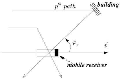
Figure 3.3.1: Scattered transmission paths and receiver’s travelling velocity $\overrightarrow{v}$

The computation for delay phase $\phi_{p}(t)$ in (3.3.2) can be carried out as follows: Denoting $v$ as velocity of mobile receiver and $\varphi_{p}$ as arriving angle of $p$th path to receiver’s moving direction [Clarke (1968)], as illustrated in Fig. 3.3.1, the delay time $\Delta\tau_{p}$ caused by each path is $\Delta\tau_{p}=\frac{\Delta x_{p}}{c}=\frac{-(v\cos\varphi_{p})t}{c}$, where $c$ is light speed and $\Delta x_{p}=-(v\cos\varphi_{p})t$ is the path length change owing to receiver’s motion [Cavers (2000)]. Then, we have:

$$\phi_{p}(t) = -2\pi f_{c}\Delta\tau_{p}=-2\pi f_{c}\frac{\Delta x_{p}}{c}$$ (3.3.3)

$$= 2\pi f_{c}\frac{(v\cos\varphi_{p})t}{c}$$

$$= 2\pi(f_{D}\mbox{$\cos\varphi_{p}$)t},\ p\in\{1,2,\ldots,K\}$$

in which the carrier Doppler shift for each path is $f_{D}\mbox{$\cos\varphi_{p}$}=$$\frac{f_{c}}{c}(v\cos\varphi_{p})$ and the frequency $f_{D}$ is often called maximum Doppler shift, since the maximum value $\cos\varphi_{p}=1$ is reached at $\varphi_{p}=0$.

In practical communication system, since the extremely-fast FFC is uncommon [Sadeghi et al. (2008)], it is safe to assume that complex fading gain will stay constant during any symbol period, i.e. $h(t)\approx h_{i}\triangleq h(iT_{s})$, in which $\frac{t}{T_{s}}\in[i-1,i)$ and $h_{i}$ is the constant fading gain during $i$th symbol period. Then, the channel waveform $g\left(t\right)$ in (3.3.1) now becomes:

$$g(t)\approx\psi(t)h_{i},\ \frac{t}{T_{s}}\in[i-1,i)$$ (3.3.4)

Applying the matched filter at carrier frequency $f_{c}$, the discrete received data in this case are:

$$x_{i} = h_{i}s_{i}+w_{i}$$

$$= \left\|h_{i}\right\|e^{j\phi_{i}}s_{i}+w_{i},\ i\in\{1,\ldots,n\}$$

Because the fading phase $\phi_{i}$ can be separately estimated along with channel synchronization, amplitude-only fading channel is a popular choice for studying fading phenomenon in the literature [Sadeghi et al. (2008)]. Then, for the amplitude-only fading scenario, which is our interest in this thesis, we have:

$$x_{i}=\left\|h_{i}\right\|s_{i}+w_{i},\ i\in\{1,\ldots,n\}$$ (3.3.5)

3.3.1 Stationary Gaussian process in fading channel

In practice, the sequence of arriving angle $\varphi_{p}$ can be modeled as uniformly iid random variable over the range $[-\pi,\pi)$ [Sadeghi et al. (2008)]. Therefore, the delay phase $\phi_{p}(t)$ in (3.3.3) is also distributed uniformly over $[-\pi,\pi)$ at anytime $t$ [Stuber (2011)]. If the number $K$ of scattering paths is sufficiently large, then owing to central limit theorem (CLT), the in-phase and quadrature components of $h(t)=h_{I}(t)+jh_{Q}(t)$ in (3.3.2) are, respectively:

$$h_{I}(t) = \sum_{p=1}^{K}\cos\phi_{p}(t)$$ (3.3.6)

$$h_{Q}(t) = \sum_{p=1}^{K}\sin\phi_{p}(t)$$

which can be approximated as independent Gaussian random variables $\mathcal{N}(0,P_{0}/2)$, where $P_{0}/2$ is called fading power per dimension [Stuber (2011)]. The average fading gain $h(t)$ is a complex WSS Gaussian process, whose autocorrelation function (ACF) is [Stuber (2011)]:

$$R_{h}(\tau) = R_{h_{I}}(\tau)+R_{h_{Q}}(\tau)$$ (3.3.7)

$$= P_{0}J_{0}(2\pi f_{D}\tau)$$

where $R_{h_{I}}(\tau)=R_{h_{I}}(\tau)=\frac{P_{0}}{2}J_{0}(2\pi f_{D}\tau)$ and $J_{0}(\cdot)$ is zero-order Bessel function of the first kind. The result (3.3.7) for Rayleigh fading channel is well known in the literature [Clarke (1968); Cavers (2000); Stuber (2011)]. However, for a quick verification, let us derive (3.3.7) briefly here. Substitute (3.3.3) to (3.3.6), we have [Stuber (2011)]:

$$R_{h_{I}}(\tau) = E[h_{I}(t)h_{I}(t+\tau)]$$

$$= \frac{P_{0}}{2}E_{\varphi_{p}}[\cos\left(2\pi(f_{D}\mbox{$\cos\varphi_{p}$)}\tau\right)]$$

owing to the central limit theorem (CLT). Then, by definition of zero-order Bessel function of the first kind, $J_{0}(x)\triangleq\frac{1}{\pi}\int_{0}^{\pi}\cos(x\sin(\varphi))d\varphi$, we have:

$$R_{h_{I}}(\tau) = \frac{P_{0}}{2}\int_{-\pi}^{\pi}\cos\left(2\pi(f_{D}\mbox{$\cos\varphi_{p}$)}\tau\right)f(\varphi_{p})d\varphi_{p}$$

$$= \frac{P_{0}}{2}\frac{1}{\pi}\int_{0}^{\pi}\cos\left(2\pi(f_{D}\mbox{$\sin\varphi_{p}$)}\tau\right)d\varphi_{p}$$

$$= \frac{P_{0}}{2}J_{0}(2\pi f_{D}\tau)$$

where $f(\varphi_{p})=\frac{1}{2\pi}$ for $\varphi_{p}\in(-\pi,\pi]$ and zero orthewise. The computation for $R_{h_{Q}}(\tau)$ is similar to $R_{h_{I}}(\tau)$, therefore we have:

$$R_{h_{Q}}(\tau)=R_{h_{I}}(\tau)=\frac{P_{0}}{2}J_{0}(2\pi f_{D}\tau)$$ (3.3.8)

The independence between $h_{I}(t)$ and $h_{Q}(t)$ can be verified by first evaluating the cross-correlation function, as follows [Stuber (2011)]:

$$R_{h_{I}h_{Q}}(\tau) = E[h_{I}(t)h_{Q}(t+\tau)]$$

$$= \frac{P_{0}}{2}E_{\varphi_{p}}[\sin\left(2\pi(f_{D}\mbox{$\cos\varphi_{p}$)}\tau\right)]$$

$$= 0$$

owing to the central limit theorem (CLT). Since $h_{I}(t)$ and $h_{Q}(t)$ are jointly Gaussian processes, the uncorrelation (orthogonal) result $R_{h_{I}h_{Q}}(\tau)=0$ is sufficient for indicating the independence of $h_{I}(t)$ and $h_{Q}(t)$, i.e.:

$$R_{h}(\tau)=R_{h_{I}}(\tau)+R_{h_{Q}}(\tau)$$ (3.3.9)

which yields (3.3.7). In the literature, this model (3.3.7) is often called Clarke’s model for fading channel, which has been widely applied in practice [Sadeghi et al. (2008)] since its first appearance in [Clarke (1968)].

Because fading gain $h(t)$ is a wide-sense stationary (WSS) process, it is possible to construct its Wold representation by infinite-order AR process, as explained in Section 2.2.4.1. A finite-order AR model does not, however, fit the above Clarke’s model, since PSD of fading gain, as computed from (3.3.7), is not a rational function of frequency [Sadeghi et al. (2008); Stuber (2011)]. Recently, a simulation of approximate Clarke’s model via high order AR model (with memory up to 1000) was considered in [Baddour and Beaulieu (2005)]. Despite small simulation error, this AR approach is prohibitive in the fading channel [Sadeghi et al. (2008)]

3.3.2 Rayleigh process in fading channel

For complex stationary Gaussian process in polar form, i.e. $h(t)=\left\|h(t)\right\|e^{j\phi(t)}$, it is also well known that the squared magnitude $\gamma\triangleq\left\|h(t)\right\|^{2}$ is a random variable with $\chi^{2}$- distribution of two degree of freedoms, as follows [Cavers (2000); Stuber (2011)]:

$$f\left(\gamma\right)=\chi_{\gamma}^{2}(2)=\frac{1}{P_{0}}\exp\left(-\frac{\gamma}{P_{0}}\right)$$ (3.3.10)

in which the mean of $\gamma$ is $E[\gamma]=E\left[\left\|h(t)\right\|^{2}\right]=P_{0}$, as in (3.3.7). Similarly, because the square-root of $\chi^{2}-$random variable in this case is a Rayleigh random variable, the distribution of magnitude $\left\|h(t)\right\|=\sqrt{\gamma}$ can be written as follows [Cavers (2000); Stuber (2011)]:

$$f\left(\left\|h(t)\right\|\right)=\frac{\left\|h(t)\right\|}{\sigma_{0}^{2}}\exp\left(-\frac{\left\|h(t)\right\|^{2}}{2\sigma_{0}^{2}}\right)$$ (3.3.11)

in which the Rayleigh squared-average is $E\left[\left\|h(t)\right\|^{2}\right]=2\sigma_{0}^{2}$. From (3.3.10), we have $\sigma_{0}^{2}=E[\gamma]/2=P_{0}/2$. Note that, because $J_{0}(0)=1$, the power average $E\left[\left\|h(t)\right\|^{2}\right]$ can also be computed by setting $\tau=0$ in autocorrelation function in (3.3.7), i.e. $\sigma_{0}^{2}=R_{h_{I}}(0)=P_{0}/2$.

Owing to standard form (3.3.11), the dominant approach in fading channel estimation is to quantize the Rayleigh distribution $f\left(\left\|h(t)\right\|\right)$ in (3.3.11) into finite cells and approximate $f\left(\left\|h(t)\right\|\right)$ via probability mass function [Sadeghi et al. (2008)]. For representing the correlated Fading process, a finite-state Markov chain (FSMC) is widely exploited, as reviewed in Section 2.3.5.3. The time-invariant transition matrix of that FSMC can be designed via quantization of jointly Rayleigh variables, as presented in Appendix B.

3.4 Summary

For modelling digital receivers, three fundamental system models were presented in this chapter.

In the first case, the synchronized scheme, the matched filter was shown to be an orthonormal correlator and, hence, preserves the sufficient statistics in the data in the case of AWGN channel.

In the second case, the un-synchronized scheme, three state-of-the-art (non-Bayesian) techniques for frequency-offset estimation were reviewed.

In the third case, the synchronized fading scheme, the derivation of the Rayleigh fading process for the amplitude of the received signal - a derivation based solely on the original Gaussian process assumption - was also presented briefly, providing us with the insight that it is actually the square-root of Chi-square process.

These models will be used, later in Chapters 7 and 8, in order to evaluate the performance of novel inference methods in this thesis.

Chapter 4 Bayesian parametric modelling

The purpose of this chapter is to show that Bayesian inference method is an effective tool for system modelling in telecommunication contexts of interest in this thesis. Since efficient computation is a major concern in mobile receivers, tractable Bayesian methods are primary concern in this chapter. Moreover, for the sake of clarity, the general form of Bayesian inference will be considered here, without any constraint on model design, while specific models of interest will be studied in later parts of this thesis.

4.1 Bayes’ rule

The aim of parametric inference is to infer some information about unknown quantity $\theta\in\Theta$, given observed data $\mathbf{x}$. For that purpose, the probabilistic solution is to impose a joint distribution $f(\mathbf{x},\theta)$ on both $\mathbf{x}$ and $\theta$. By probabilistic chain rule, $f(\mathbf{x},\theta)$ can be factorized into two equivalent ways, as follows:

$$f(\theta|\mathbf{x})f(\mathbf{x}) = f(\mathbf{x},\theta)$$ (4.1.1)

$$= f(\mathbf{x}|\theta)f(\theta)$$

Hence, any information that data $\mathbf{x}$ can provide us about $\theta$ must be contained within the posterior distribution $f(\theta|\mathbf{x})$. Because the value $\mathbf{x}$ is known, the data inference $f(\mathbf{x})=\int f(\mathbf{x},\theta)d\theta$, also known as predictive inference or occasionally as the evidence [Bernardo and Smith (1994)], is regarded as normalizing constant for posterior distribution $f(\theta|\mathbf{x})$, as follows:

$$f(\theta|\mathbf{x}) = \frac{f(\mathbf{x}|\theta)f(\theta)}{f(\mathbf{x})}$$ (4.1.2)

$$\propto f(\mathbf{x}|\theta)f(\theta)$$

where $\propto$ denotes normalizing operator, i.e. the right hand side of $\propto$ is normalized to be sum-to-one over $\theta$. The well-known formula (4.1.2) is called Bayes’ rule in the literature. Important texts on Bayes’ theory and calculus are found in [Bernardo and Smith (1994); Jaynes (2003); Robert (2007)].

4.2 Subjectivity versus Objectivity

Despite simplicity, Bayes’ rule raises a philosophical issue on subjectivity of probability, which is perhaps the most critical issue in Bayesian inference [Robert (2007)]. The most popular criticism is to regard the prior and posterior distributions objectively, i.e. as a measure of a repeatable or generable quantity, rather than “quantification of belief” about $\theta$ in Bayesian philosophy [Bernardo and Smith (1994)].

Putting Bayesian interpretation aside, it can be seen that both prior and posterior models are simply consequences of joint model $f(\mathbf{x},\theta)$ design (4.1.1), which is subjective per se. Box’s famous comment that “all models are wrong, but some are useful” [Box (1979a)] was also stated as “models are never true, but it is only necessary that they are useful” [Box (1979b)]. The usefulness is, therefore, a necessary and subjective criterion for model design. Hence, in order to avoid the philosophical ambiguity between objectivity and subjectivity of probability (see e.g. [Lindley (2000)] and discussions therein), in this thesis, the imposed joint model $f(\mathbf{x},\theta)$ is considered as subjective belief, while the prior and posteriors are considered as deductive consequences of the subjective modelling. The justification is the following:

- Regarding subjectivity: In deterministic model, the purpose of parametric inference is to return the optimal estimate $\widehat{\theta}$ such that a criterion like loss function $\mathcal{L}\triangleq L(\mathbf{x},\theta)$ can be minimized at $\widehat{\theta}$. In probability context, the distribution $f(\mathcal{L})$ is, therefore, a transformation of $f(\mathbf{x},\theta)$. Since joint model $f(\mathbf{x},\theta)$, regardless of repeatability or unrepeatability, is fundamentally imposed by our belief on the system, it is obviously subjective and need to be useful under criterion $L(\mathbf{x},\theta)$.

- Regarding objectivity: Note that chain rule of factorization in (4.1.1) follows the Axioms of Probability [Bernardo and Smith (1994)], i.e. the computation of prior and posterior would never change the originally set-up joint model $f(\mathbf{x},\theta)$. Hence, the term “Bayesian inference” in this thesis simply refers to computation of posterior distribution in (4.1.2), rather than its Bayesian subjectivity meaning. Bayesian inference is, at least in this thesis, a mathematical technique to solve the above subjective problem.

4.3 Bayesian estimation as a Decision-Theoretic task

Owing to Bayes’ rule (4.1.2), the data information about $\theta$ is all contained in posterior distribution $f(\theta|\mathbf{x})$. In practice, however, the desired output is often a single point estimation or decision $\xi\triangleq\widehat{\theta}\left(\mathbf{x}\right):\mathcal{X}\rightarrow\Theta$ of $\theta\in\Theta$. In this section, Bayesian criteria for optimizing value $\xi$ will be reviewed.

4.3.1 Utility and loss function

The utility and loss definition was often expressed in different forms in different fields. In this subsection, let us review some of these forms, before applying the approach to Bayesian estimator in the consequence.

In decision theory, a chosen action $a(\theta):\Theta\rightarrow\mathcal{A}$, defined as a function of event $\theta$, is justified by a gain or benefit of that action. The measure of that benefit is called utility, denoted $u(a(\theta))$, whose axiomatization is firstly presented in [von Neumann and Morgenstern (1944)].

In statistical decision, however, the action $a$ is typically chosen via a loss, i.e. negative utility, firstly formalized by Wald [Wald (1949)]:

$$L_{u}(a,\theta)=-u(a(\theta))$$ (4.3.1)

where $L_{u}(a,\theta):\mathcal{A}\times\Theta\rightarrow\mathbb{R}$. The key role of definition (4.3.1) is that the action $a$ is now regarded as independent of parameter event $\theta$ in $L_{u}(a,\theta)$. Moreover, in order to guarantee a non-negative loss action, the loss definition in (4.3.1) is further constrained into a (regret) loss function, as follows [Parmigiani and Inoue (2009)]:

$$L\left(a,\theta\right)\triangleq L_{u}(a,\theta)-\inf_{a\in\mathcal{A}}L_{u}(a,\theta)$$ (4.3.2)

where $L\left(a,\theta\right):\mathcal{A}\times\Theta\rightarrow\mathbb{R}_{\geq 0}$.

In parametric inference, the action $a$ is to pick a value $\xi$ in parameter space $\Theta$, i.e. $a=\xi\in\mathcal{A}=\Theta$. By this way, the definition (4.3.2) becomes a loss function $\mathcal{L}\triangleq L(\xi,\theta)$ for estimator $\xi$ of $\theta$ such that $L(\xi,\theta):\Omega\times\Omega\rightarrow\mathbb{R}_{\geq 0}$ and $L(\xi,\theta)=0\Leftrightarrow\xi=\theta$. In deterministic scenario, the standard criterion is to pick the value $\widehat{\xi}$ of $\xi$ such that the loss function is minimized, i.e. we have:

$$\widehat{\xi}=\arg\min_{\xi\in\Theta}L(\xi,\theta)$$

.

Lastly, in probability context, the estimator $\xi$ is assigned as a function of data $\xi\triangleq\widehat{\theta}\left(\mathbf{x}\right):\mathcal{X}\rightarrow\Omega$ in a functional space $\xi\in\Xi$ . In this context, the value $\mathcal{L}=L(\xi,\theta)=L\left(\widehat{\theta}\left(\mathbf{x}\right),\theta\right)$ is a deterministic function of two random variables $\{\mathbf{x},\theta\}$. Then, the aim of parametric inference in this case is to pick the minimum risk (MR) function $\widehat{\xi}=\widehat{\theta}_{MR}(\mathbf{x})$ in functional space $\Xi$ such that the expected loss function is minimized, i.e. we have:

$$\widehat{\theta}_{MR}(\mathbf{x})=\arg\min_{\widehat{\theta}\left(\cdot\right)\in\Xi}E_{f(\mathcal{L})}L\left(\widehat{\theta}\left(\mathbf{x}\right),\theta\right)$$ (4.3.3)

In general, a loss function $\mathcal{L}$ can be designed via definition of gain function (4.3.1), via definition of regret function (4.3.2), by system requirement or simply by imposing tractably mathematic form. Then, theoretically, the distribution $f(\mathcal{L})$ in (4.3.3), $\mathcal{L}\in\mathbb{R}_{\geq 0}$, can be derived via transformation of joint distribution $f(\mathbf{x},\theta)$. However, in practice, the exact form of $f(\mathcal{L})$ is often difficult to compute. The most common solution is to confine ourself to expected loss function $\bar{\mathcal{L}}\triangleq E_{f(\mathcal{L})}(\mathcal{L})$. For this reason, a theory of functional mean will be briefly reviewed first, before we derive the computation of that mean value $\bar{\mathcal{L}}$.

4.3.1.1 Expectation of a function

In probability theory, law of the unconscious statistician (LOTUS) is important [Ghahramani (2005)]. Historically, the term “unconscious” was used because some people forgot that this law was not a definition [Ross (1970); Schervish (1995)], although some statisticians, e.g. [Casella and Berger (2002)], did not find that term amusing. The virtue of LOTUS is that we can compute the expected value of a deterministic function $\psi=g\left(\theta\right)$ from original distribution $f(\theta)$, without the need of computing transformed distribution $f(\psi)$, which might be difficult to carry out in practice.

Proposition 4.3.1.

(Law of unconscious statistician (LOTUS)) (see e.g. [Wong and Hajek (1985); Ghahramani (2005)] for rigorous proof)

If $\theta$ is a random variable with probability function $f(\theta)$ and $\psi=g\left(\theta\right):\Theta\rightarrow\mathbb{R}$ is a measurable function, then $E_{f(\psi)}(\psi)=E_{f(\theta)}(g\left(\theta\right))=\int g\left(\theta\right)f(\theta)d\theta$.

Somewhat relevant to LOTUS is the concept of certainty equivalent (CE) in decision theory, defined as follows:

Definition 4.3.2.

(Certainty Equivalent) [Parmigiani and Inoue (2009)] The certainty equivalent $\widehat{\theta}_{CE}\in\Theta$, if existent, is a special value of $\theta\in\Theta$, such that:

$$g\left(\widehat{\theta}_{CE}\right)=E_{f(\theta)}g\left(\theta\right)$$ (4.3.4)

The equation (4.3.4) means that expectation of functional form can be evaluated by a single CE point $\widehat{\theta}_{CE}$, if that CE exists. Note that, the sufficient condition for existence of $\widehat{\theta}_{CE}$ is that $g\left(\theta\right)$ is linear with $\theta$ (4.3.4).

4.3.2 Bayes risk

By Proposition 4.3.1, the expected value $\bar{\mathcal{L}}$ in (4.3.3) can be found via the joint distribution $f(\mathbf{x},\theta)$, as follows:

$$\bar{\mathcal{L}}\triangleq E_{f(\xi,\theta)}L(\xi,\theta)=E_{f(\mathbf{x},\theta)}L(\widehat{\theta}\left(\mathbf{x}\right),\theta)$$ (4.3.5)

In the literature, the expected loss in (4.3.5) is also called Bayes risk [Berger (1985)]. In practice, because the computation of expectation (4.3.5) via joint distribution $f(\mathbf{x},\theta)$ is often not in closed form, the Bayesian risk (4.3.5) can be estimated via empirical (Monte Carlo) sampling of $f(\mathbf{x},\theta)$.

4.3.2.1 Posterior expected loss

The MR estimator $\widehat{\theta}_{MR}\triangleq\widehat{\theta}_{MR}(\mathbf{x})$ in (4.3.3) can also be found via posterior expected loss function, without the need of computing the form $f(\mathbf{x},\theta)$. By factorization $f(\mathbf{x},\theta)=f(\mathbf{x})f(\theta|\mathbf{x})$ in (4.1.1), the Bayesian risk (4.3.5) can also be computed by averaging posterior distribution, i.e.: $\bar{\mathcal{L}}=E_{f(\mathbf{x})}\left\{E_{f(\theta|\mathbf{x})}L(\widehat{\theta}\left(\mathbf{x}\right),\theta)\right\}$ . Since $f(\mathbf{x})\geq 0$ for any $\mathbf{x}$, we have an equivalent way to find the optimal estimator $\widehat{\theta}_{MR}$ in (4.3.3), as follows:

$$\widehat{\theta}_{MR}=\arg\min_{\widehat{\theta}\left(\cdot\right)}E_{f(\theta|\mathbf{x})}L\left(\widehat{\theta}\left(\mathbf{x}\right),\theta\right)$$ (4.3.6)

Hence, an advantage of Bayesian estimation method is that deriving optimal estimator $\widehat{\theta}_{MR}$ via posterior distribution $f(\theta|\mathbf{x})$ is often much more feasible than via joint distribution $f(\mathbf{x},\theta)$ [Berger (1985)].

4.3.2.2 Minimum risk estimators

From (4.3.6), it is feasible to derive the optimal estimators for several well-known loss functions. For example, if $L(\widehat{\theta},\theta)$ is quadratic loss $\left\|\widehat{\theta}-\theta\right\|_{2}^{2}$, zero-one loss $\delta(\widehat{\theta}-\theta)$ or scalar absolute loss $\left\|\widehat{\theta}-\theta\right\|_{1}$, the minimum risk estimator $\widehat{\theta}_{MR}$ is the mean, mode or median of posterior distribution $f(\theta|\mathbf{x})$, respectively [Berger (1985)].

In information theory, the Hamming distance is an important function. Generally, a Hamming loss can be defined for continuous case, as follows:

$$L\left(\widehat{\theta},\theta\right)\equiv Q(\widehat{\theta},\theta)=1-\frac{1}{n}\sum_{i=1}^{n}\delta\left(\widehat{\theta}_{i}-\theta_{i}\right)$$ (4.3.7)

where $\widehat{\theta}=\{\widehat{\theta}{}_{1},\widehat{\theta}{}_{2},\ldots,\widehat{\theta}_{n}\}$ is the set of estimates and $\theta=\{\theta{}_{1},\theta{}_{2},\ldots,\theta_{n}\}$ is the set of parameters. The Hamming loss in (4.3.7) can be minimized via the following Lemma:

Lemma 4.3.3.

The minimum risk (MR) estimate $\widehat{\theta}_{MR}=\{\widehat{\theta}_{1}(\mathbf{x}),\ldots,\widehat{\theta}_{n}(\mathbf{x})\}$, which minimizes $E_{f(\mathbf{x},\theta)}Q(\widehat{\theta},\theta)$, is the sequence of marginal MAP:

$$\widehat{\theta}_{i}(\mathbf{x})=\arg\max_{\theta_{i}}f(\theta_{i}|\mathbf{x}),\ i\in\{1,2,\ldots,n\}$$ (4.3.8)

Proof.

From (4.3.7), we can see that the MR estimate for Hamming loss is:

$$\min_{\widehat{\theta}(\cdot)}E_{f(\theta|\mathbf{x}_{n})}L\left(\widehat{\theta}(\mathbf{x}),\theta\right) = 1-\frac{1}{n}\sum_{i=1}^{n}\max_{\widehat{\theta}(\cdot)}E_{f(\theta|\mathbf{x}_{n})}\delta\left(\widehat{\theta}_{i}(\mathbf{x})-\theta_{i}\right)$$ (4.3.9)

$$= 1-\frac{1}{n}\sum_{i=1}^{n}\max_{\theta_{i}}f(\theta_{i}|\mathbf{x})$$

which yields (4.3.8). ∎

In the literature, a special case of Lemma 4.3.3, in which $\theta$ is discrete and Dirac-$\delta(\cdot)$ is replaced by Kronecker-$\delta[\cdot]$, is proved in [Winkler (1995); Lember (2011)]. The above proof is provided in this thesis in order to cover the case of continuous r.v. $\theta$.

4.4 Bayesian inference

As explained in subsection 4.3.2.1, although the ultimate aim of estimation task is to minimize the Bayesian risk $\bar{\mathcal{L}}$ (4.3.5) via joint model $f(\mathbf{x},\theta)$, the Minimum Risk (MR) estimated decision (4.3.6) can be found equivalently via posterior distribution $f(\theta|\mathbf{x})$. The tractable computation of posterior is, therefore, the main interest in this thesis.

Because the joint model $f(\mathbf{x},\theta)$ depends on the design of observation part $f(\mathbf{x}|\theta)$ and the prior part $f(\theta)$, the technical issues with those two parts will be reviewed first in this section. The role of posterior part $f(\theta|\mathbf{x})$, which is a mere consequence of the chain rule (4.1.1), will then be reviewed.

4.4.1 Observation model

In contrast to the deterministic approach, the probabilistic approach considers the observed data $\mathbf{x}$ as one realization of observation distribution $f(\mathbf{x}|\theta)$, given a shaping parameter $\theta$. In other words, the parametric model $f(\cdot|\theta)$ is a quantization model of the observer’s/modeller’s belief about the possible realization $\mathbf{x}$, of $\mathbf{X}$, when observed.

For clarifying potential confusion, let us emphasize again that, in this thesis, the data $\mathbf{x}$ is regarded as one and only one realization, drawn from $f(\mathbf{x}|\theta)$. Owing to this convention, it does not matter whether the random quantity $\mathbf{x}$ is repeatable or unrepeatable. In stochastic case where there are $n$ observed data, the notation $\mathbf{x}$ will be specialized to $\mathbf{x}_{n}\triangleq\{x{}_{1},x{}_{2},\ldots,x_{n}\}$.

In practice, the observation model $f(\mathbf{x}|\theta)$ is often imposed by physical laws. In mathematical models, $f(\mathbf{x}|\theta)$ can be flexibly parameterized by exploiting exchangeability, invariance or sufficiency properties of data $\mathbf{x}$ [Bernardo and Smith (1994)]. In that theoretical context, $f(\mathbf{x}|\theta)$ often belongs to standard distributions, which are derived from experiments or defined in probability textbooks [Kotz et al. (1997, 2004a, 2004b, 2005)].

For computational efficiency, the data sufficiency is the most important property for us to exploit. If a statistic, i.e. a function of data, extracts information on its parameter partially, a sufficient statistic is much more efficient since it can extract that information fully. Furthermore, sufficient statistics can represent the whole data in a parametric model and, hence, might reduce the data complexity significantly. For that reason, the parameterization technique via sufficient statistics and its typical class, namely Exponential Family, is the key in this thesis and will be briefly reviewed in this chapter.

4.4.1.1 Sufficient statistics

The sufficient statistics of an observation model $f(\mathbf{x}|\theta)$ can be identified via a well-known criterion, as follows:

Proposition 4.4.1.

(Fisher-Neyman factorization criterion) The statistics $\mathcal{\tau}(\mathbf{x})$ is called sufficient if and only if the observation distribution can be factorized as [Bernardo and Smith (1994)]:

$$f(\mathbf{x}|\theta)=h\left(\mathcal{\tau}(\mathbf{x}),\theta\right)g\left(\mathbf{x}\right)$$ (4.4.1)

for some functions $h\left(\cdot\right)\geq 0$ and $g\left(\cdot\right)>0$.

Because the parameter $\theta$ only interacts with data $\mathbf{x}$ via function $h\left(\mathcal{\tau}(\mathbf{x}),\theta\right)$ in (4.4.1), all the information of data $\mathbf{x}$ regarding $\theta$ is summarized in $\mathcal{\tau}(\mathbf{x})$, hence its name sufficient statistic.

In history, the notion of sufficient statistics was firstly defined in [Fisher (1922)], while the factorization (4.4.1) is explicitly established in [Neyman (1935)]. In classical inference, the sufficient statistics plays an important role, mostly owing to Rao-Blackwell-Kolmogorov theorem [Blackwell (1947); Kolmogorov (1950); Rao (1965)], which establishes that unbiased estimators based on sufficient statistic are the best estimators. In Bayesian inference, however, sufficient statistics are simply regarded as a consequence of the Bayesian method [Bernardo and Smith (1994)]. Owing to Bayes’ rule (4.1.2) and Neyman factorization (4.4.1), the posterior inference normalizes out any data factor $g\left(\mathbf{x}\right)$ irrelevant to parameter and, hence, always exploits the minimal sufficient statistics [Lehmann and Casella (1998)].

Nevertheless, the sufficiency principle plays a central role for data simplification of two major observation classes: transformation family (TF) and exponential family (EF). Indeed, most standard distributions, see e.g. [Kotz et al. (1997, 2004a, 2004b, 2005)], belong to just these two classes [Lehmann and Casella (1998)]. The former extracts sufficient statistics of interesting parameters via a group of transformations, such as scaling or location shift, while, on the other hand, preserving the original distribution’s structure [Cox (2006)]. The latter reduces data complexity, regardless of sample size, to a fixed (usually small) number of sufficient statistics without loss of information [Lehmann and Casella (1998)]. Since EF class is widely exploited in signal processing for tractable computation, it will be reviewed in this chapter. Some distributions in TF class, namely spherical distributions, that also belong to EF class will be presented as an application in Section 7.3.

4.4.1.2 Exponential Family

In the class of distributions parameterized via sufficient statistics, the most important is the exponential family (EF), firstly pioneered by [Darmois (1935); Koopman (1936); Pitman and Wishart (1936)]. The first motivation of the EF class is to exploit the fixed-dimension property of sufficient statistics, as stated via Darmois-Koopman-Pitman theorem [Andersen (1970)]: “Under regularity conditions, a necessary and sufficient condition for the existence of a sufficient statistic of fixed dimension is that the probability density belongs to the exponential family”. Following up that result, the sufficient data reduction in the EF class was then studied thoroughly in [Andersen (1970); Brown (1986)]. The main motivation for EF’s usage nowadays is simply the computational tractability engendered in the posterior distribution [Robert (2007)].

Definition 4.4.2.

(Exponential Family) The observation model $f(\mathbf{x}|\theta)$ is a member of EF if and only if there is a separability between parameters and data kernels, as follows [Brown (1986)]:

$$f(\mathbf{x}|\theta)=C(\theta)h\left(\mathbf{x}\right)\exp\left(R(\theta)\mathcal{\tau}(\mathbf{x})\right)$$ (4.4.2)

In a more relaxed form, the scalar product $R(\theta)\mathcal{\tau}(\mathbf{x})$ in (4.4.2) might be replaced by a scalar product $\left\langle R(\theta),\mathcal{\tau}(\mathbf{x})\right\rangle$ that is linear in the second argument (such as the Euclidean inner product in the case where $R(\theta)$ and $\mathcal{\tau}(\mathbf{x})$ are vector structures of equal dimension) [Smidl and Quinn (2006); Nielsen and Garcia (2009)].

Comparing (4.4.1) with (4.4.2), we recognize that the data kernel $\mathcal{\tau}(\mathbf{x})$ is a sufficient statistic in EF. Moreover, $\mathcal{\tau}(\mathbf{x})$ is also invariant with increasing numbers of observation. For example, given an iid sequence $\mathbf{x}_{n}=\{x{}_{1},x{}_{2},\ldots,x_{n}\}$, the EF observation (4.4.2) becomes $f(\mathbf{x}_{n}|\theta)=\prod_{i=1}^{n}f(x_{i}|\theta)=C(\theta)^{n}h\left(\mathbf{x}_{n}\right)\exp\left(R(\theta)\mathcal{\tau}(\mathbf{x}_{n})\right)$, where the sufficient statistic $\mathcal{\tau}(\mathbf{x}_{n})=\sum_{i=1}^{n}\mathcal{\tau}(x_{i})$ preserves the dimension of initial statistics $\mathcal{\tau}(x_{1})$.

Note that, if we regard the empirical mean $\frac{1}{n}\mathcal{\tau}(\mathbf{x}_{n})$ as a moment constrain of iid sequence $\mathbf{x}_{n}=\{x{}_{1},x{}_{2},\ldots,x_{n}\}$, the EF form (4.4.2) can also be found via maximum entropy (MaxEnt) principle [Wainwright and Jordan (2008)].

4.4.2 Prior distribution

As explained above, the prior design $f(\theta)$ cannot be separated from the design of joint model $f(\mathbf{x},\theta)$, which, in turn, depends on the data characteristics. Hence, the goodness of estimation does not only rely on inference techniques, but also on the quality of model design. For any optimal decision, the first and foremost question is whether we have considered all possible options, since too narrow a set of options might lead us to a sub-optimal solution at best [Box (1979b)]. The aim of prior design is, therefore, to embrace all possibilities of parameter for the data set in the joint model.

In practice, there are three scenarios for prior design:

- If we have no information on $\theta$ a priori, a non-informative approach will be applied to prior design (see e.g [Kass and Wasserman (1996)] for full review and bibliography of this approach). The most well-known priors in this case are uniform prior (also known as Laplace’s prior) [Laplace (1814)], Jeffreys’ prior [Jeffreys (1946)] and reference prior [Bernardo (1979)], as reviewed below.

- If we have all information on $\theta$, i.e. the prior distribution is already given along with joint model, there is nothing for us to do. However, if only the form of prior is defined, the prior design becomes a tuning problem on shaping parameters of that form. An example of this case is a conjugate prior, as explained below. Another example is the multinomial distribution, which is the uniquely available form for any discrete compact-support random variable. This multinomial prior will be considered in Section 6.2.

- If we have access to partial information on $\theta$, such as moments or some constraints, a distributional optimizer can be sought. For this case, some approximation methods, e.g. MaxEnt or moments matching, can be applied [Robert (2007)]. These approximations will be explained in Section 4.4.2.5.

In this subsection, the typical priors for those three cases will be briefly reviewed. Laplace’s prior, which is ignorant to data characteristics, will be presented first in order to recall the ignorance principle in prior design.

4.4.2.1 Uniform prior

The earliest principle, dated back to [Laplace (1814)], in prior design is the “principle of indifference” (also called “principle of insufficient reason” or Laplace’s rule [Kass and Wasserman (1996)]), which imposes a uniform prior. This principle, however, receives some serious criticism. Firstly, the uniform distribution is improper for non-compact support $\theta$. Secondly and more fundamentally, the principle of indifference ignores the re-parameterization issue in observation model, which contains all the information of data about parameter. Without taking that issue into account, the non-informative prior $f(\theta)$ for a posteriori estimation on $\theta$ might become an informative prior $f(\psi)$ for a posteriori estimation on $\psi$, where $\psi=g\left(\theta\right)$ is a one-to-one mapping.

4.4.2.2 Jeffreys’ prior

In order to preserve the non-informative property in the re-parmeterization issue, a criterion, namely “invariance under re-parameterization”, was originally required in Jeffreys’ prior [Jeffreys (1946)].

Given observation model $f(\mathbf{x}|\theta)$, the Fisher information is defined as follows: $I\left(\theta\right)\triangleq E_{f(\mathbf{x}|\theta)}$$\left(\frac{\partial\log f(\mathbf{x}|\theta)}{\partial\theta}\right)^{2}$. Owing to Jacobian transformation, the Fisher information is actually invariant under re-parameterization, as follows: $I\left(\theta\right)=I\left(\psi\right)\left(\partial\psi/\partial\theta\right)^{2}$, where $\psi=g\left(\theta\right)$ is a one-to-one mapping. Because square-root of $I\left(\theta\right)$ yields a distributional transformation, the Jeffreys prior is defined as $f(\theta)\propto\sqrt{I\left(\theta\right)}$. In the case of multi-dimensional parameter, the Jeffrey prior becomes $f(\theta)\propto\sqrt{\det\{I\left(\theta\right)\}}$, where $I\left(\theta\right)$ is the Fisher information matrix.

Nevertheless, Jeffreys’ prior is often improper, particularly in the multi-dimensional case. For this reason, Jeffreys’ prior is considered as intuitive proposal, rather than a practical approach [Bernardo and Smith (1994)].

4.4.2.3 Reference prior

A Bayesian, and somewhat objective, approach for prior design is to consider the relationship between posterior and prior distributions, given a fixed observation model. The criterion for optimal estimation is, as explained above, to maximize the range of possibilities that the prior can contribute to the posterior distribution. The reference prior, firstly proposed in [Bernardo (1979)], solved this problem via a variational approach, as follows:

$$f(\theta)=\arg\max_{f(\theta)}\left\{E_{f(\mathbf{x})}KLD\left(f(\theta|\mathbf{x})||f(\theta)\right)\right\}$$

where KLD denotes Kullback-Leibler divergence [Cover and Thomas (2006)]:

$$KLD\left(\tilde{f}(\theta)||f(\theta)\right)\triangleq E_{\tilde{f}(\theta)}\log\frac{\tilde{f}(\theta)}{f(\theta)}\geq 0$$ (4.4.3)

If $\theta$ is scalar and continuous, the reference prior is identical to Jeffreys’ prior [Bernardo and Smith (1994)], but this is not true in the multi-dimensional case.

4.4.2.4 Conjugate prior

Another method for prior design is conjugate principle, which preserves the prior and posterior within the same functional class, as follows:

Definition 4.4.3.

(Conjugacy) [Robert (2007)] A prior distribution $f(\theta|\eta)\in\mathcal{F}$ in distributional class $\mathcal{F}$ is called conjugate to an observation $f(\mathbf{x}|\theta)$ if its posterior distribution also belongs to $\mathcal{F}$, i.e. the distributional form is closed under Bayes’ rule (4.1.2).

Owing to conjugacy, the data update for posterior parameter can be computed directly within data space itself, while the distributional form stays unchanged.

In particular, this invariance property under Bayes’ rule plays a central role in tractable and efficient computation for the EF class. Indeed, because the EF observation model (4.4.2) preserves data dimension, the dimension of its conjugate prior’s parameters, which are defined within the same data space, is also preserved a posteriori.

Definition 4.4.4.

(CEF class) The conjugate prior for EF observation model, which we call the CEF distribution, can be defined as follows:

$$f(\theta|\eta_{0})=C(\theta)^{\nu_{0}}\exp\left(R(\theta)v_{0}\right)$$ (4.4.4)

where $\eta_{0}=\{\nu_{0},v_{0}\}$ is the shaping parameter.

Obviously, the initialization of $\eta_{0}$ makes conjugate prior somewhat informative, although special values of $\eta_{0}$ can make conjugate EF prior identical to the non-informative Jeffrey prior in some standard distributions.

4.4.2.5 MaxEnt Prior

Let us assume that, a priori, there is a set of mean constraints on the parameter, as follows:

$$f(\theta)\in\mathcal{F}_{m}:\ E_{f(\theta)}g_{i}(\theta)=m_{i}$$ (4.4.5)

where all $m_{i}$ are known and $\mathcal{F}_{m}$ is the set of constrained distributions. The Maximum Entropy (MaxEnt) principle, implied by [Jaynes (1980, 1983)], chooses the prior $\tilde{f}(\theta)\in\mathcal{F}_{m}$ whose entropy $\mathcal{E}_{f(\theta)}$ is maximized, i.e. $\tilde{f}(\theta)=\arg\max_{f(\theta)\in\mathcal{F}_{m}}\mathcal{E}_{f(\theta)}$ (once again, a variational principle).

For defining entropy, however, there are two distinct cases. In the discrete case, the entropy is traditionally defined as: $\mathcal{E}_{f(\theta)}=-\sum_{\theta_{k}\in\Theta}f(\theta_{k})\log f(\theta_{k})$. In the continuous case, the relative Entropy is preferred, i.e. $\mathcal{E}_{f(\theta)}=-KLD(f(\theta)||f_{0}(\theta))$, where $f_{0}(\theta)$ is a reference distribution. In practice, $f_{0}(\theta)$ might be designed as reference prior above. The differential entropy, i.e. integration form of discrete Entropy $\mathcal{E}_{f(\theta)}=-\int_{\theta}f(\theta)\log f(\theta)d\theta$, is not always applicable in continuous case since it is sometimes negative.

The MaxEnt solution $\tilde{f}(\theta)$ for discrete and continuous cases are $\tilde{f}(\theta)\propto\exp\left(-\sum_{i}g_{i}(\theta)\lambda_{i}\right)$ and $\tilde{f}(\theta)\propto\exp\left(-\sum_{i}g_{i}(\theta)\lambda_{i}\right)f_{0}(\theta)$, respectively, where $\lambda_{i}$ are Lagrange multipliers of the mean constraints (4.4.5). With those forms, we can recognize that MaxEnt prior $\tilde{f}(\theta)$ is also a member of CEF class (4.4.4).

4.4.3 Posterior distribution

Given both observation and prior above, the joint model $f(\mathbf{x},\theta)$ is already properly defined, and, hence, the computation of posterior distribution in (4.1.2) is straight forward. In this subsection, the main advantages of posterior distribution as an inference object will be briefly reviewed and compared with other inference techniques.

4.4.3.1 Predictive inference

Firstly, let us recall that, the predictive model $f(\mathbf{x})$ on observable $\mathbf{x}$ can be represented by marginalization over all possible values of its parameter, as follows:

$$f(\mathbf{x})=\int f(\mathbf{x}|\theta)f(\theta)d\theta$$

Similarly, the posterior predictive model $f(y|\mathbf{x})$ on observable $y$, given data $\mathbf{x}$, can be represented via marginalization over posterior distribution, as follows:

$$f(y|\mathbf{x})=\int f(y|\mathbf{x},\theta)f(\theta|\mathbf{x})d\theta$$ (4.4.6)

From (4.4.6), we can see that posterior $f(\theta|\mathbf{x})$ can be used as intermediate step to derive the inference $f(y|\mathbf{x})$ for unknown quantity $y$. This simple, yet elegant, form of Bayesian prediction (4.4.6) has been used extensively in density estimation [Aitchison and Dunsmore (1980)], data classification [Lavine and West (1992); Klein and Press (1992)], model checking [Gelman et al. (1996); Gelman et al. (2003)], model averaging [Raftery et al. (1995)], etc.

Note that, in the frequentist approach, because prior part $f(\theta)$ is missing, the prediction (4.4.6) has to rely on plug-in approximation $\tilde{f}(\theta|\mathbf{x})=\delta(\theta-\widehat{\theta})$, sometimes referred to as a CE approximation:

$$\tilde{f}(y|\mathbf{x}) = \int f(y|\mathbf{x},\theta)\delta(\theta-\widehat{\theta})d\theta$$ (4.4.7)

$$= f(y|\mathbf{x},\widehat{\theta})$$

where $\widehat{\theta}$ is often chosen as the Maximum Likelihood (ML) estimate, i.e. $\widehat{\theta}=\arg\max_{\theta\in\Theta}f(\mathbf{x}|\theta)$ (see e.g. [Aitchison and Dunsmore (1980)] for the details). In the model-selection problem, such a substitution is also popular, i.e. parameter model is often chosen first, before the prediction step is carried out, although this approach is often criticized for neglecting model uncertainty (see e.g. [Raftery et al. (1995)] and discussion therein).

4.4.3.2 Hierarchical and nuisance parameters

In the case of binary partition $\theta=\{\theta_{i},\theta_{\backslash i}\}$, where $\theta_{i}$ is the parameter of interest and $\theta_{\backslash i}$ is the nuisance parameter, the Bayesian inference for $\theta_{i}$ can be readily derived via posterior $f(\theta|\mathbf{x})$, as follows:

$$f(\theta_{i}|\mathbf{x}) = \int f(\theta|\mathbf{x})d\theta_{\backslash i}$$ (4.4.8)

$$\propto \int f(\mathbf{x}|\theta)f(\theta)d\theta_{\backslash i}$$

By substituting the chain rule $f(\theta)=f(\theta_{\backslash i}|\theta_{i})f(\theta_{i})$ into (4.4.8), we can also derive a Bayes’ rule for $\theta_{i}$ directly, as follows:

$$f(\theta_{i}|\mathbf{x})\propto f(\mathbf{x}|\theta_{i})f(\theta_{i})$$

where:

$$f(\mathbf{x}|\theta_{i}) = \int f(\mathbf{x}|\theta)f(\theta_{\backslash i}|\theta_{i})d\theta_{\backslash i}$$ (4.4.9)

$$= \int f(\mathbf{x},\theta_{\backslash i}|\theta_{i})d\theta_{\backslash i}$$

Note that this nuisance parameter issue is more difficult to solve with frequentist method. Since prior $f(\theta)$ is missing in this case, the marginalization in (4.4.9) has to be approximated. The common solution is to apply plug-in method, i.e. the nuisance $\theta_{\backslash i}$ is replaced by its point estimation $\widehat{\theta_{\backslash i}}$, which yields the so-called profile likelihood [Bernardo and Smith (1994)], as follows:

$$f_{p}(\mathbf{x}|\theta_{i}) = f(\mathbf{x}|\theta_{i},\widehat{\theta_{\backslash i}})$$ (4.4.10)

where again, $\widehat{\theta_{\backslash i}}$ is typically chosen via ML principle. From (4.4.8) and (4.4.9), we can see that the Bayesian inference for any subset of parameters can be found by marginalizing out all nuisance parameters. However, this approach often yields a complicated conditional distribution which is often intractable [Liseo (2006)]. From (4.4.9), note that $f(\mathbf{x}|\theta_{i})$ is an infinite mixture of full observation model $f(\mathbf{x}|\theta)$, with mixing density $f(\theta_{\backslash i}|\theta_{i})$.

Another approach is to produce an asymptotic integrated likelihood via reference prior [Berger and Bernardo (1992); Liseo (1993)]. A major difficulty is that this approach depends strongly on an order of parameters, which is relevant to the ordered grouping problem [Bernardo and Smith (1994)].

In the $n$-ary partition $\theta=\{\theta{}_{1},\theta{}_{2},\ldots,\theta_{n}\}$, the direct computation of (4.4.8) is not feasible in general [Gelman et al. (2003)]. This case is called hierarchical parameter in the literature and will be studied in Section 6.2.

4.4.3.3 Sufficient statistics and shaping parameters

From Fisher-Neyman factorization (4.4.1), it is feasible to recognize that, owing to normalizing operator in Bayes’ rule (4.1.2), the posterior inference for $\theta$ only depends on sufficient statistic, rather than the whole data, as follows:

$$f(\theta|\mathcal{\tau}(\mathbf{x}))\propto f(\mathbf{x}|\theta)f(\theta)$$

Hence, $\mathcal{\tau}(\mathbf{x})$ now becomes a shaping parameter for the posterior distribution $f(\theta|\mathbf{x})$. In a slightly more general case, where the prior $f(\theta|\eta)$ depends on known hyper-parameter $\eta$ (also called shaping parameter in this thesis), the posterior form can be written as follows:

$$f(\theta|\eta(\mathbf{x}))\propto f(\mathbf{x}|\theta)f(\theta|\eta)$$

where $\eta(\mathbf{x})=\{\mathcal{\tau}(\mathbf{x}),\eta\}$ is called (data-updated) shaping parameter for the posterior.

The main challenges for posterior tractability are, therefore, to identify the sufficient statistic and to design a prior such that the computation of $\eta(\mathbf{x})$ is feasible. Both of them can be feasibly solved via definition of EF class. Multiplying the conjugate prior (4.4.4) with EF observation (4.4.2), the conjugate posterior can be feasibly derived, as follows:

$$f(\theta|\eta_{1}(\mathbf{x}))\propto C(\theta)^{\nu_{1}}\exp\left(R(\theta)v_{1}(\mathbf{x})\right)$$ (4.4.11)

where $\nu_{1}=\nu_{0}+1$, $v_{1}(\mathbf{x})=v_{0}+\mathcal{\tau}(\mathbf{x})$ and $\eta_{1}(\mathbf{x})=\{\nu_{1},v_{1}(\mathbf{x})\}$. Note that, because the dimension of EF sufficient statistic $\mathcal{\tau}(\mathbf{x}_{n})=\sum_{i=1}^{n}\mathcal{\tau}(x_{i})$ is preserved in iid case $\mathbf{x}_{n}=\{x{}_{1},x{}_{2},\ldots,x_{n}\}$, the computation of posterior’s shaping parameter $\eta_{1}(\mathbf{x})$ is always tractable. Hence, the EF class plays an important role in tractable Bayesian inference. In the online scheme, the computation of $\mathcal{\tau}(\mathbf{x}_{n})$ can be carried out recursively [Smidl and Quinn (2006)].

4.4.3.4 Asymptotic inference

Let us consider the negative logarithm of posterior distribution $\mathrm{L}(\theta)=-\log f(\theta|\mathbf{x}_{n})$ expanded up to second order of Taylor approximation, as follows:

$$\mathrm{L}(\theta)=\mathrm{L}(\theta_{0})+(\theta-\theta_{0})^{\prime}\nabla\mathrm{L}(\theta_{0})-\frac{1}{2}(\phi-\phi_{0})^{\prime}\mathrm{H}(\theta_{0})(\theta-\theta_{0})+\ldots$$ (4.4.12)

where $\nabla\mathrm{L}(\theta_{0})$ and $\mathrm{H}(\theta_{0})=-\nabla^{2}\mathrm{L}(\theta_{0})$ are the gradient vector and Hessian matrix evaluated at vector point $\theta=\theta_{0}$, respectively, assuming regularity conditions on $\mathrm{L}(\theta)$ [Bernardo and Smith (1994)]

In the special case of the iid observation model, the first two orders of the Taylor expansion yields an asymptotically converged form for posterior distribution, as follows:

Proposition 4.4.5.

(Asymptotic posterior normality) [Bernardo and Smith (1994)] Given iid observation model $f(\mathbf{x}_{n}|\theta)=\prod_{i=1}^{n}f(x_{i}|\theta)$ and maximum a posteriori (MAP) $\widehat{\theta}$, i.e. $\nabla\mathrm{L}(\widehat{\theta})=0$, then under regularity conditions, the posterior distribution $f(\theta|\mathbf{x}_{n})$ converges to the normal distribution $\mathcal{N}_{\theta}\left(\widehat{\theta},\mathrm{H}^{-1}(\widehat{\theta})\right)$, when $n\rightarrow\infty$.

The asymptotic posterior normality was firstly proposed and rigorously proved in [Laplace (1810)] and [Le Cam (1953)], respectively. Note that, given the iid observation model, we also have a special converged form $\mathrm{H}(\widehat{\theta}_{ML})\rightarrow n\mathcal{I}(\widehat{\theta}_{ML})$ as $n\rightarrow\infty$, where $\widehat{\theta}_{ML}=\arg\max_{\theta}f(\mathbf{x}_{n}|\theta)$ [Gelman et al. (2003); Bernardo and Smith (1994)]. However, unless the prior is uniform, the posterior $f(\theta|\mathbf{x})$ does not necessarily converge to $\mathcal{N}_{\theta}\left(\widehat{\theta}_{ML},\mathrm{H}^{-1}(\widehat{\theta}_{ML})\right)$.

4.5 Distributional approximation

The computation of posterior distribution $f(\theta|\mathbf{x})$ is obviously the main focus of Bayesian theory. However, the computation of the posterior form via Bayes’ rule (4.1.2) is often intractable in practice. A common solution is, therefore, to use distributional approximation $\tilde{f}(\theta|\mathbf{x})$ of $f(\theta|\mathbf{x})$, in which the form $\tilde{f}(\theta|\mathbf{x})$ is tractable. The tractability means that the computation can be carried out via a closed-form formula and/or can be determined analytically in polynomial time.

The study of such approaches was the main reason for the revival of Bayesian methodology in the 1980s. In this subsection, the most important approximations will be briefly reviewed.

4.5.1 Deterministic approximations

4.5.1.1 Certainty equivalence (CE) approximation

When moments of $f(\theta|\mathbf{x})$ are needed, but posterior form is hard to derive, we can confine the posterior distribution into a single point $\widehat{\theta}(\mathbf{x})$, as follows:

$$\tilde{f}(\theta|\mathbf{x})=\delta(\theta-\widehat{\theta}(\mathbf{x}))$$ (4.5.1)

Note that, by the sifting property, the functional moments $\widehat{g\left(\theta\right)}=E_{f(\theta|\mathbf{x})}g\left(\theta\right)$ can be approximated via substitution, as follows:

$$\widehat{g\left(\theta\right)} \approx E_{\tilde{f}(\theta|\mathbf{x})}g\left(\theta\right)$$

$$= E_{\delta(\theta-\widehat{\theta}(\mathbf{x}))}g\left(\theta\right)$$

$$= g\left(\widehat{\theta}(\mathbf{x})\right)$$ (4.5.3)

In the literature, this approximation (4.5.3) is widely known as the plug-in substitution technique [Robert (2007)]. However, it will be called the Certainty Equivalent (CE) approximation in this thesis, owing to its expectation form in (4.5.1.1) and the fact that it encodes all the uncertainty about $\theta$ a posteriori by a single value $\widehat{\theta}(\mathbf{x})$ (4.5.1). Although this CE approximation concept (4.5.1.1) is different from the exact solution via CE principle (4.3.4), they will coincide if we can assign the CE, i.e. $\widehat{\theta}(\mathbf{x})=\widehat{\theta}_{CE}(\mathbf{x})$, in (4.5.1) that satisfies (4.3.4). The name CE hence reflects the concept of distributional representation via a representative value. In practice, $\widehat{\theta}(\mathbf{x})$ is often chosen as the mean, mode, median of posterior distribution $f(\theta|\mathbf{x})$, or as other minimum risk estimates (4.3.6).

4.5.1.2 Laplace approximation

Owing to asymptotic posterior normality in Proposition 4.4.5, the posterior $f(\theta|\mathbf{x})$ can be approximated via its asymptotic form, i.e. $\tilde{f}(\theta|\mathbf{x})=\mathcal{N}_{\theta}\left(\widehat{\theta},\mathrm{H}^{-1}(\widehat{\theta})\right)$, where $\widehat{\theta}$ is the MAP estimate (mode) of $f(\theta|\mathbf{x})$. The quality of this approximation obviously depends on the number of observations and is typically poor in small samples.

4.5.1.3 MaxEnt approximation

The posterior $f(\theta|\mathbf{x})$ can also be approximated via MaxEnt technique in Section 4.4.2.5, if distributional class $f(\theta|\mathbf{x})\in\mathcal{F}_{m}$ (4.4.5) is already given. Similarly to derivation of MaxEnt prior, the MaxEnt posterior $\tilde{f}(\theta|\mathbf{x})\in\mathcal{F}_{m}$ is also a member of CEF class, as follows:

$$\tilde{f}(\theta|\mathbf{x})\propto\exp(-\sum_{i}g_{i}(\theta)\lambda_{i}(\mathbf{x}))$$ (4.5.4)

where Lagrangre multipliers $\lambda_{i}(\mathbf{x})$ depend on data $\mathbf{x}$ in this case. Note that, MaxEnt is a free-form variational technique, since CEF form (4.5.4) of $\tilde{f}(\theta|\mathbf{x})$ is not fixed during approximation, but merely a solution of free-form Entropy maximization process.

4.5.2 Variational Bayes (VB) approximation

In this thesis, the main deterministic approximation is the free-form (variational) VB approximation. Let us provide a brief review of VB and its variants in this subsection.

4.5.2.1 Mean field theory

The term “variational” originates from the term “calculus of variations” [Choudrey (2002)], in which the (optimum) value of a definite integral (or a functional) deterministically depends on the function in the argument of that integral [Stephenson and Radmore (1990)]. The idea of the VB approximation has its roots in mean field theory (MFT), which is originally a statistical quantum mechanics term, although the definition of MFT was not specific in that early era [Callen (1985)]. Loosely speaking, the MFT originally represents a technique for approximating an interacting particle model by another non-interacting particle model, such that the Helmholz free-energy is corrected up to the first order [Callen (1985)]. The MFT was later defined as a deterministic approximation for the expected value of individual quantities in a generic statistical model, as firstly introduced in neural networks in [Peterson and Anderson (1987)].

In Bayesian learning, the MFT was called “ensemble learning” [MacKay (1995)] and re-defined as an approximate distribution, from a class of “separable” (i.e. independent) variables, to an arbitrary distribution, such that the “variational free-energy” from the approximate distribution to original distribution is minimized. The MFT was then, once again, re-defined as the Variational Bayes method [Attias (1999); Jaakkola and Jordan (2000)], which minimizes the variational free-energy via the iterative Expectation-Maximization (EM) and an iterative EM-like algorithm, called the VB EM algorithm [Beal (2003)]. Note that, the methods based on variational free-energy above mostly focus on point estimates and neglect the optimization of the distributional form within the class of approximate distributions of independent variables.

Finally, the VB methodology was properly defined in [Smidl and Quinn (2006)] as a free-form distributional approximation in the class of independent variables, such that the Kullback-Leibler divergence (KLD) from the approximate distribution to the original distribution is minimized. An Iterative VB (IVB) algorithm was also proposed in [Smidl and Quinn (2006)] in order to reach the local minimum of the KLD via an iterative gradient-based method. Because this free-form definition of VB approximation is more consistent with Bayesian methodology, this thesis will adopt this VB approach.

4.5.2.2 Iterative VB algorithm

Let us consider a binary partition of parameters $\theta=\{\theta_{i},\theta_{\backslash i}\}$, where $\theta_{\backslash i}$ denotes the complement of $\theta_{i}$ in $\theta$, i.e. the joint model $f(\mathbf{x},\theta)$ has the following form:

$$f(\mathbf{x},\theta)=f(\mathbf{x},\theta_{i},\theta_{\backslash i})$$ (4.5.5)

Then, the purpose of VB method is to seek an approximated distribution $\tilde{f}(\theta|\mathbf{x})\in\mathcal{F}_{c}$ in independent distribution class $\mathcal{F}_{c}:\ \breve{f}(\theta|\mathbf{x})=\breve{f}(\theta_{i}|\mathbf{x})\breve{f}(\theta_{\backslash i}|\mathbf{x})$, for which the Kullback-Leibler divergence $KLD_{\breve{f}||f}\triangleq KLD(\breve{f}(\theta|\mathbf{x})||f(\theta|\mathbf{x}))=E_{\breve{f}(\theta|\mathbf{x})}\log\left(\frac{\breve{f}(\theta|\mathbf{x})}{f(\theta|\mathbf{x})}\right)$ is minimized.

Theorem 4.5.1.

(Iterative VB (IVB) algorithm) [Smidl and Quinn (2006)] Given an arbitrary initial distribution $\tilde{f}^{[0]}(\theta|\mathbf{x})=\tilde{f}^{[0]}(\theta_{i}|\mathbf{x})\tilde{f}^{[0]}(\theta_{\backslash i}|\mathbf{x})$, the IVB algorithm updates VB-marginals in iterative cycle $\nu=1,2,\ldots$ until $KLD_{\tilde{f}||f}$ is converged to a local minimum, as follows:

$$\tilde{f}^{[\nu]}(\theta_{i}|\mathbf{x}) \propto \exp(E_{\tilde{f}^{[\nu-1]}(\theta_{\backslash i}|\mathbf{x})}\log f(\mathbf{x},\theta))$$ (4.5.6)

$$\tilde{f}^{[\nu]}(\theta_{\backslash i}|\mathbf{x}) \propto \exp(E_{\tilde{f}^{[\nu]}(\theta_{i}|\mathbf{x})}\log f(\mathbf{x},\theta))$$

Note that, because $\tilde{f}^{[\nu]}(\theta|\mathbf{x})$ in IVB algorithm (4.5.6) results from a gradient-based technique, convergence to the global minimum is not guaranteed [Smidl and Quinn (2006)]. Hence, $\tilde{f}^{[\infty]}(\theta|\mathbf{x})$ is a local minimizer of $KLD_{\breve{f}||f}$.

In practice, the computation of expectation in IVB algorithm (4.5.6) might be prohibitive or intractable. There are, however, some cases in which this intractability can be avoided, as presented below.

4.5.2.3 Separable-in-parameter (SEP) family

From IVB cycles (4.5.6), it is feasible to recognize that there exists a tractable class of joint distribution, such that the IVB algorithm is tractable, as follows:

Definition 4.5.2.

(Separable-in-parameter (SEP) family) [Smidl and Quinn (2006)] The joint distribution $f(\mathbf{x},\theta)$ is said to belong to SEP family if its sub-parameters can be split between separated kernels $g\left(\cdot\right)$and $h\left(\cdot\right)$, as follows:

$$\log f(\mathbf{x},\theta)=g\left(\theta_{i},\mathbf{x}\right)h\left(\theta_{\backslash i},\mathbf{x}\right)$$ (4.5.7)

Substituting the joint model (4.5.7) back into (4.5.6), the IVB scheme now becomes:

$$\tilde{f}^{[\nu]}(\theta_{i}|\mathbf{x}) \propto \exp\left(g\left(\theta_{i},\mathbf{x}\right)\widehat{h\left(\theta_{\backslash i},\mathbf{x}\right)}^{[\nu-1]}\right)$$ (4.5.8)

$$\tilde{f}^{[\nu]}(\theta_{\backslash i}|\mathbf{x}) \propto \exp\left(\widehat{g\left(\theta_{i},\mathbf{x}\right)}^{[\nu]}h\left(\theta_{\backslash i},\mathbf{x}\right)\right)$$

where the iterative functional moments (called the VB moments) are defined as:

$$\widehat{h\left(\theta_{\backslash i},\mathbf{x}\right)}^{[\nu-1]} \triangleq E_{\tilde{f}^{[\nu-1]}(\theta_{\backslash i}|\mathbf{x})}h\left(\theta_{\backslash i},\mathbf{x}\right)$$

$$\widehat{g\left(\theta_{i},\mathbf{x}\right)}^{[\nu]} \triangleq E_{\tilde{f}^{[\nu]}(\theta_{i}|\mathbf{x})}g\left(\theta_{i},\mathbf{x}\right)$$

From (4.5.8), we can see that VB marignals are available if the VB moments can be computed. The advantage of the separability constant is that these computations remain invariant (i.e. the integral in each VB moment is not a function of $\nu$). In this thesis, we are only interested in SEP family for the IVB algorithm, owing to this tractability property.

Note that, similar to the Exponential Family (4.4.2), the key motivation of the SEP family is to exploit the separability between functional variables in order to achieve the tractability in integral computation. In the former case, the computation in normalizing constant is solved via separability between parameters and observed data. In the latter case, the computation in IVB expectation is feasible owing to separability between sub-parameters, given observed data.

4.5.2.4 Functionally constrained VB (FCVB) approximation

Another solution for tractably computing (4.5.6) is to project one or all of the VB-marginals $\tilde{f}^{[\nu]}(\theta_{\backslash i}|\mathbf{x})$, $\tilde{f}^{[\nu]}(\theta_{i}|\mathbf{x})$ into functionally constrained classes $f_{\delta}^{[\nu]}(\theta_{\backslash i}|\mathbf{x})$, $f_{\delta}^{[\nu]}(\theta_{i}|\mathbf{x})$, in particular the CE class (4.5.1), before they are used in the expectation step of the IVB cycle (4.5.6). This approximation scheme is called the FCVB approximation.

In this way, the well-known Expectation-Maximization (EM) algorithm can be recognized as a special case of FCVB, in which $\tilde{f}^{[\nu]}(\theta_{\backslash i}|\mathbf{x})$ is projected to its local MAP point $\widehat{\theta_{\backslash i}}$, i.e. $f_{\delta}^{[\nu]}(\theta_{\backslash i}|\mathbf{x})=\delta(\theta_{\backslash i}-\widehat{\theta_{\backslash i}}^{[\nu]})$, while $\tilde{f}^{[\nu]}(\theta_{i}|\mathbf{x})$ is kept unchanged [Smidl and Quinn (2006)].

Similarly, another form of FCVB is when both VB-marginals $\tilde{f}^{[\nu]}(\theta_{\backslash i}|\mathbf{x})$, $\tilde{f}^{[\nu]}(\theta_{i}|\mathbf{x})$ are each projected into their local MAP point $f_{\delta}^{[\nu]}(\theta_{\backslash i}|\mathbf{x})=\delta(\theta_{\backslash i}-\widehat{\theta_{\backslash i}}^{[\nu]})$, $f_{\delta}^{[\nu]}(\theta_{i}|\mathbf{x})=\delta(\theta_{i}-\widehat{\theta_{i}}^{[\nu]})$, respectively, as follows:

Lemma 4.5.3.

(Iterative FCVB algorithm) Given an arbitrary initial value $\widehat{\theta}^{[0]}=\{\widehat{\theta_{i}}^{[0]},$ $\widehat{\theta_{\backslash i}}^{[0]}\}$, the distribution $f_{\delta}^{[\nu]}(\theta|\mathbf{x})\in\mathcal{F}_{\delta}:\ \breve{f_{\delta}}(\theta)=\delta(\theta_{i}-\widehat{\theta_{i}})\delta(\theta_{\backslash i}-\widehat{\theta_{\backslash i}})$ that locally minimizes $KLD(f_{\delta}(\theta|\mathbf{x})||f(\theta|\mathbf{x}))$ can be found via Iterative FCVB algorithm at cycle $\nu=1,2,\ldots,$ as follows:

$$\widehat{\theta_{i}}^{[\nu]} = \arg\max_{\theta_{i}}(\exp(E_{f_{\delta}^{[\nu-1]}(\theta_{\backslash i}|\mathbf{x})}\log f(\mathbf{x},\theta)))$$

$$= \arg\max_{\theta_{i}}f(\mathbf{x},\theta_{i},\theta_{\backslash i}=\widehat{\theta_{\backslash i}}^{[\nu-1]})$$

$$\widehat{\theta_{\backslash i}}^{[\nu]} = \arg\max_{\theta_{\backslash i}}(\exp(E_{f_{\delta}^{[\nu]}(\theta_{i}|\mathbf{x})}\log f(\mathbf{x},\theta)))$$

$$= \arg\max_{\theta_{\backslash i}}f(\mathbf{x},\theta_{i}=\widehat{\theta_{i}}^{[\nu]},\theta_{\backslash i})$$

Proof.

By definition, we have:

$$KLD(f_{\delta}(\theta|\mathbf{x})||f(\theta|\mathbf{x}))=E_{f_{\delta}(\theta|\mathbf{x})}\log\left(\frac{f_{\delta}(\theta|\mathbf{x})}{f(\theta|\mathbf{x})}\right)=\log\left(\frac{1}{f(\theta=\widehat{\theta}|\mathbf{x})}\right)$$

owing to the sifting property of $f_{\delta}(\theta|\mathbf{x})=\delta(\theta-\widehat{\theta})$. The local minimization can be seen intuitively by comparing (4.5.3) with (4.5.5). The value of posterior at any $\widehat{\theta}$, i.e. $f(\theta=\widehat{\theta}|\mathbf{x})=f(\mathbf{x},\theta=\widehat{\theta})/f(\mathbf{x})$, does not decrease at any step in (4.5.3). Hence, the value of $KLD(f_{\delta}(\theta|\mathbf{x})||f(\theta|\mathbf{x}))$ is locally minimized at a local MAP $\widehat{\theta}$ at the convergence. ∎

Note that, the Iterative FCVB is not a double approximation, i.e. it is not an approximation of VB approximation. Both IVB and Iterative FCVB schemes are local minimizers of KLD distance from an independent class, namely $\mathcal{F}_{c}$ and $\mathcal{F}_{\delta}$, respectively, to the original distribution. However, because of similarity between (4.5.6) and (4.5.3), the Iterative FCVB approximation is considered as variant of IVB approximation in this thesis.

It can be seen that the iterative CE updates (4.5.3) in FCVB algorithm is identical to Iterated Conditional Modes (ICM) algorithm [Besag (1986)], which is well known to yield a local joint MAP estimate $\widehat{\theta}=\{\widehat{\theta_{i}},\widehat{\theta_{\backslash i}}\}$ of original distribution $f(\theta|\mathbf{x})$ at convergence [Dogandzic and Zhang (2006)]. Nevertheless, the name “Iterative FCVB algorithm” is preferred to “ICM algorithm” in this thesis, since performance of this scheme is easier to explain via independence property of distributional VB approximation.

4.5.2.5 Non-iterative VB-related approximations

In the literature, there are other non-iterative approximations that can be considered as variants of the VB scheme. Although they will not be used in this thesis, let us briefly review three typical cases for the sake of completeness.

- If the purpose of the approximation is to minimize $KLD_{MR}\triangleq KLD(f(\theta|\mathbf{x})||\tilde{f}(\theta|\mathbf{x}))$ instead of $KLD_{\tilde{f}||f}$ in the VB scheme, the minimizer in this case is $\tilde{f}(\theta|\mathbf{x})$ $=$ $f(\theta_{i}|\mathbf{x})$ $f(\theta_{\backslash i}|\mathbf{x})$, i.e. the product of true posterior marginals. This scheme is widely known as Minimum Risk (MR) approximation.

- Obviously, the above MR approximation may not be interesting, since those posterior marginals may be hard to compute in the first place. However, if one posterior marginal, say $f(\theta_{\backslash i}|\mathbf{x})$, is given, the VB-marginal $\tilde{f}(\theta_{i}|\mathbf{x})$ can be found by a single step of IVB algorithm (4.5.6), with $\tilde{f}(\theta_{\backslash i}|\mathbf{x})$ replaced by the true marginal $f(\theta_{\backslash i}|\mathbf{x})$. This non-iterative scheme is called the Quasi-Bayes approximation in the literature.

- If the true marginal $f(\theta_{\backslash i}|\mathbf{x})$ in above Quasi-Bayes scheme is not given, we can still replace $\tilde{f}(\theta_{\backslash i}|\mathbf{x})$ with a restricted form $\overline{f}(\theta_{\backslash i}|\mathbf{x})$ , which can be imposed via some constraints on $\theta_{\backslash i}$. Such a single-step VB scheme is called Restricted VB approximation.

4.5.3 Stochastic approximation

A wide class of distributional approximation is the stochastic approximation, in which the posterior $f(\theta|\mathbf{x})$ can be empirically approximated, as follows:

$$\tilde{f}(\theta|\mathbf{x})=\frac{1}{m}\sum_{k=1}^{m}\delta(\theta-\theta^{(k)})$$ (4.5.10)

where $\{\theta^{(1)},\theta^{(2)},\ldots,\theta^{(m)}\}$ is an iid sample set (random sample), i.e. $\theta^{(k)}\sim f(\theta|\mathbf{x})$, with $k\in\{1,2,\ldots,m\}$.

In low dimensions, the generation of $\theta^{(k)}$ can be implemented via a wide range of sampling techniques, notably inversion, rejection and importance sampling. In inversion sampling, the value $F^{(k)}$ of cumulative function density (c.d.f) $F(\theta)\in[0,1]$ is generated first, while the scalar random variable $\theta$ can be found via inverse function $F^{-1}$, i.e. $\theta^{(k)}=F^{-1}(F^{(k)})$. In rejection sampling, the sample $\theta^{(k)}\sim f_{0}(\theta)$ is generated from the so-called dominated distribution $f_{0}(\theta)\geq f(\theta)$, $\forall\theta\in\Theta$ and, then, each sample $\theta^{(k)}$ is accepted with probability $p_{k}=f(\theta^{(k)})/f_{0}(\theta^{(k)})$ or else rejected. In importance sampling, we have $\tilde{f}(\theta)=\frac{1}{m}\sum_{k=1}^{m}w_{k}\delta(\theta-\theta^{(k)})$ , where each sample $\theta^{(k)}\sim\pi(\theta)$ is generated from a reference distribution $\pi(\theta)$ and the weights are computed as $w_{k}=f(\theta^{(k)})/\pi(\theta^{(k)})$.

In high dimensions, the set $\{\theta^{(1)},\theta^{(2)},\ldots,\theta^{(m)}\}$ can be generated dependently via a homogeneous Markov process $f(\theta_{k}|\theta_{k-1})$. After a transition period $k_{c}$, the set $\{\theta^{(k)},\ldots,$ $\theta^{(m)}\}$, $k>k_{c}$, is converged to iid sampling set of $f_{s}(\theta)$, where $f_{s}(\theta)$ is, under mild regularity conditions, the stationary distribution of homogeneous Markov process $f(\theta_{k}|\theta_{k-1})$. This convergence in distribution is independent of initialization $\theta^{(1)}$of this Markov process, known as the forgetting property. By careful design of Markov transition kernel $f(\theta_{k}|\theta_{k-1})$, we can achieve the equality $f_{s}(\theta)=f(\theta)$. This is the basic principle of Gibbs sampling in Markov Chain Monte Carlo (MCMC) method [Geman and Geman (1984)]. Another well known technique for designing transition kernel in MCMC is Metropolis–Hastings algorithm [Metropolis et al. (1953)], whose stationary distribution is the objective distribution. The key advantage of MCMC is that an intractably high-dimensional distribution can be tractably generated from multiple sampling steps of low-dimensional conditional distributions.

The most important condition of this technique is obviously the repeatability of $\theta$. Then, owing to the sifting property of the Dirac-$\delta$ function, all functional moments of the empirical approximation, $\tilde{f}(\theta|\mathbf{x})$, in (4.5.10) can be point-wise evaluated and, hence, are always tractable. In prediction or online schemes, where the current posterior becomes prior of next Bayesian inference step, the empirical form (4.5.10) also satisfies the conjugacy principle, and, hence, is always tractable. This idea is at the heart of particle filtering for stochastic approximation of the nonlinear filtering problem for time-variant parameters [Smidl and Quinn (2008)]. For reducing computational load, some variants of particle filtering, which do not require a re-sampling step, were recently proposed in the telecommunications context [Yua and Zhengb (2011); Ghirmai (2013)].

4.6 Summary

A brief, but thorough, review for Bayesian techniques was given in this chapter. It began with emphasis on the joint model, rather than the posterior distribution, along with clarification on the issue of subjectivity in belief quantification.

Initially, the expectation of the loss function was taken with respect to the joint model of parameters and data, via the axioms of decision theory, and not with respect to the posterior distribution. The law of the unconscious statistician (LOTUS) then showed that the mean of loss function for the joint model, i.e. Bayesian risk, can be approximated by Monte Carlo sampling and presented in simulation (e.g. as averaged BER). Since Bayesian risk can be minimized equivalently via the minimum risk (MR) estimator for posterior expected loss function, this motivated the review of the posterior distribution, which, in turn, motivated the reviews of prior and observation models, particularly the conjugacy property in this chapter.

Some distributional approximations, both deterministic and stochastic, were surveyed, with a thorough review of VB and its special case, functionally constrained VB (FCVB), for reducing Kullback-Leibler divergence (KLD) associated with approximate distribution. These VB-based methods will be used for designing novel algorithms in the context of the hidden Markov chain for digital receivers, in Chapters 6.

Chapter 5 Generalized distributive law (GDL) for CI structure

A typical scenario in Bayesian inference is the marginalization over hierarchical and nuisance parameters, as shown in Section 4.4.3.2. Such a computation can be efficiently computed via the generalized distributive law (GDL), as explained in this chapter. This GDL scheme will also reveal efficient algorithms for Markovian model, i.e. a special case of conditionally independent (CI) model, in Chapter 6.

5.1 Introduction

When computing a sequence of operators upon a product of multivariate functions (factors), the generalized distributive law (GDL) [Aji and McEliece (2000)] has been proposed for reducing the computational load. Nevertheless, the proposed computational flow of GDL has to be designed via a graph representation of those factors.

In this chapter, we will propose a novel topology representation, namely conditional independent (CI) structure, for those factors. This topology divides the factors into separate partitions, across which the operators can be freely distributed via GDL. Because two design stages, one for factors and one for operators, are isolated in this scheme, the total number of arithmetic operators can be tuned feasibly. This flexibility is useful for designing an optimal reduction in computational complexity.

5.1.1 Objective functions

In order to be consistent with the literature, the standard notation $\{\cdot,\cdot,\ldots,\cdot\}$ for a set with separated partitions will be applied throughout this chapter. Then, let $\mathbf{x}_{\Omega}$ be $m$-tuples variables within $\mathcal{X}_{\Omega}$ space, i.e. $\mathbf{x}_{\Omega}=\{x_{1},\dots,x_{m}\}\in\mathcal{X}_{\Omega}$, where $\Omega$ is the total index set (universe), as follows:

$$\Omega\triangleq\{1,\ldots,k,\ldots,m\}$$ (5.1.1)

and dimension is equal to its cardinality. For simplicity, let us assume here that all $x_{k}$ belong to the same finite set $\mathcal{X}$, i.e. $x_{k}\in\mathcal{X}_{k}=\mathcal{X}$, $k=1,\ldots,m$, and hence:

$$\mathbf{x}_{\Omega}\in\mathcal{X}_{\Omega}\triangleq\underset{m\ times}{\underbrace{\mathcal{X}\times\ldots\times\mathcal{X}}}=\mathcal{X}^{m}$$ (5.1.2)

We also denote:

$$M \triangleq |\mathcal{X}|$$ (5.1.3)

$$m \triangleq |\Omega|$$

where $|\cdot|$ is the cardinal number of a finite set. Note that all the results in this chapter can be generalized feasibly to the case of different sets $\mathcal{X}_{k}$ and/or the case of continuous variables [Pakzad and Anantharam (2004)].

Throughout this chapter, let us define $g:\mathcal{X}^{|\omega|}\rightarrow\mathbb{R}$ as a generic (i.e. wildcard) function $g$ over index set $\omega\subseteq\Omega$ of variables $\mathbf{x}_{\omega}$. Then, as an imposed model, the main function, $g(\mathbf{x}_{\Omega})$, is assumed to be a product of $n$ known factors, as follows:

$$g(\mathbf{x}_{\Omega})=\prod_{i=1}^{n}g(\mathbf{x}_{\omega_{i}})$$ (5.1.4)

where index sets are defined as $\omega_{i}\subseteq\Omega=\{1,\ldots,m\}$ and $\omega_{i}\neq\emptyset$, $i=1,2,\ldots,n$, such that:

$$\Omega=\omega_{1}\cup\cdots\cup\omega_{n}$$ (5.1.5)

For shortening notation in (5.1.4), let us also denote $\mathbf{g}_{1:n}\triangleq g(\mathbf{x}_{\Omega})$ and $g_{i}\triangleq g(\mathbf{x}_{\omega_{i}})$, which yield a neater form:

$$\mathbf{g}_{1:n}\equiv\prod_{i=1}^{n}g_{i}=g(\mathbf{x}_{\Omega})$$ (5.1.6)

Finally, if we define a generic operator ring-product $\odot$ from ring theory (see Definition 5.3.4) instead of product $\prod$, the model (5.1.6) can be treated generally as follows:

$$\mathbf{g}_{1:n}\equiv\odot_{i=1}^{n}g_{i}=g(\mathbf{x}_{\Omega})$$ (5.1.7)

For illustration, several examples of (5.1.6) in this thesis are (4.5.7), (6.2.2.1) (see e.g. [Moon (2005)] for more examples in telecommunication context).

For later use, let us propose the following definition:

Definition 5.1.1.

(Index of variable and index set of factor)
The index $k\in\Omega$ in (5.1.1) is called index of variable (or variable index). In (5.1.4-5.1.5), $\omega_{i}$ is called the index set of the factor $g_{i}$ (or the factor index set of $g_{i}$) in (5.1.6-5.1.7).

5.1.1.1 Single objective function

In practice, it is often required to compute a sequence of operators upon a sequence of factors $\mathbf{g}_{1:n}$ (5.1.6). For example, the objective function might be the output of summation:

$$\sum_{\mathbf{x}_{S}}\mathbf{g}_{1:n}=\sum_{\mathbf{x}_{S}}g(\mathbf{x}_{\Omega})=g(\mathbf{x}_{\mathcal{S}^{c}})$$

or maximization:

$$\max_{\mathbf{x}_{S}}\mathbf{g}_{1:n}=\max_{\mathbf{x}_{S}}g(\mathbf{x}_{\Omega})=g(\mathbf{x}_{\mathcal{S}^{c}})$$

where $\mathbf{x}_{\Omega}=\{\mathbf{x}_{\mathcal{S}^{c}},\mathbf{x}_{S}\}$ and:

$$\Omega=\{\mathcal{S}^{c},\mathcal{S}\}$$ (5.1.8)

Nevertheless, a generic operator ring-sum $\boxplus_{\mathbf{x}_{\mathcal{S}}}$ from ring theory (Definition 5.3.3) over $\mathbf{x}_{\mathcal{S}}$ is not necessarily the sum or max. The objective function $g(\mathbf{x}_{\mathcal{S}^{c}})$ is then defined as the output of that operator upon $\mathbf{g}_{1:n}$ in (5.1.7), as follows:

$$\boxplus_{\mathbf{x}_{\mathcal{S}}}\mathbf{g}_{1:n}=\boxplus_{\mathbf{x}_{\mathcal{S}}}g(\mathbf{x}_{\Omega})=g(\mathbf{x}_{\mathcal{S}^{c}})$$ (5.1.9)

When dimension $m$ (5.1.2) is too high, the task (5.1.9) leads to a heavy computational load in practice [Aji and McEliece (2000); Moon (2005)].

For later use, let us propose the following definition:

Definition 5.1.2.

(Index set of operator $S$ and objective set $\mathcal{S}^{c}$)
In (5.1.8), the set $S\subseteq\Omega$ is called the index set of operators (or operator index set) and the compliment $\mathcal{S}^{c}=\Omega\backslash\mathcal{S}$ is called the objective set (of objective function).

5.1.1.2 Sequential objective functions

In practice, it is more often required to compute a sequence of objective functions, rather than a single objective function. In this case, the sequential objective functions can be defined as:

$$\boxplus_{\mathbf{x}_{\mathcal{S}_{j}}}\mathbf{g}_{1:n}=\boxplus_{\mathbf{x}_{\mathcal{S}_{j}}}g(\mathbf{x}_{\Omega})=g(\mathbf{x}_{\mathcal{S}^{c}_{j}}),\ j=1,2,\ldots,\kappa,$$ (5.1.10)

in which:

$$\Omega=\{\mathcal{S}^{c}_{1},\mathcal{S}_{1}\}=\ldots=\{\mathcal{S}^{c}_{\kappa},\mathcal{S}_{\kappa}\}$$ (5.1.11)

In a naive approach, we merely apply the computation (5.1.9) $\kappa$ times, each time with different operator index set $\mathcal{S}_{j}$. The computational load is, loosely speaking, about $\kappa$-fold the computational cost in (5.1.9). Because we often have $\kappa=n$ , this approach becomes impractical for high $n$.

For efficient computation, we confine ourselves to a special topological case, defined below (Definition 5.2.8) as the non-overflowed condition for the objective sets $\{\mathcal{S}^{c}{}_{1},\mathcal{S}^{c}{}_{2},\ldots,\mathcal{S}^{c}_{\kappa}\}$. The results of the $\kappa$ formulae in (5.1.10) can be extracted, in a single sweep, from computational memory of a single objective function (5.1.9) upon a union of operator index sets, $\mathcal{S}=\mathcal{S}_{1}\cup\ldots\cup\mathcal{S}_{\kappa}$ (hence the name “sequential functions”), if that extraction does not require any re-computation step and does not yield overflowed memory (hence the name “non-overflowed”). Note that, as shown below, the case of scalar objective sets $\mathcal{S}^{c}_{j}=j$, which is widely required in practice, always satisfy this condition.

5.1.2 GDL - the state-of-the-art

If the two operators, $\boxplus$ and $\odot$, satisfy distributive law of ring theory (Definition 5.3.2), the total number of these operators in sequential objective functions (5.1.10) can be reduced significantly, as firstly formalized in [Aji and McEliece (2000)] for the case of scalar objective sets $\mathcal{S}^{c}_{j}=j$. Such a proposal motivated practical studies of the generalized distributive law (GDL) in ring theory in order to design efficient algorithms [Glazek (2002)]. Nevertheless, the use of GDL in the literature is still modest. The main effort in the literature so far is to re-interpret known efficient algorithms for sum and max operators into ring theory, which, in turn, can generalize those algorithms for all operators $\boxplus$ satisfying GDL, as briefly reviewed below.

In the early days, the main interest is to generalize some probabilistic computational algorithms on the joint distribution $f(\mathbf{x}_{\Omega})$ into ring theory. For example, two well-known algorithms (in Chapter 6) in Markov Chain decoder context - the Viterbi algorithm (VA) for joint maximum-a-posteriori (MAP) and the Forward-Backward (FB) algorithm (also known as BCJR algorithm in channel decoder context) for sequence of marginal MAP [Moon (2005)] - were generalized in [Fettweis and Meyr (1990)] and [Wiberg (1996); McEliece (1996)], respectively. In Bayesian networks, the generalized forms of belief propagation and message-passing algorithms for a sequence of marginals were proposed in [Nielsen (2001); Kschischang et al. (2001)].

Recently, the primary interest in GDL comes from graph theory. The trend can be considered as having begun with the semi-tutorial paper [Aji and McEliece (2000)], which migrated the early results into graphical learning language. GDL for graph was also applied in other fields, like circuit design [Tong and Lam (1996)], automatics [Hardouin et al. (2010)] and entropy computation in probability [Ilic et al. (2011)]. However, a drawback for GDL development in graph theory has been the inconsistency of the semiring concept, which is still under development in modern algebra [Glazek (2002)]. Only recently, an attempt at unifying the ring concepts for graphs was proposed in [Gondran and Minoux (2008)].

5.1.3 The aims of this chapter

From the above review, we can feasibly grasp the reason for emergence of GDL in graph theory: the key point is that the graph provides a structure representation of the original model (5.1.7). From that structure, the operators are then distributed directly into factors $g_{i}$ via GDL. The computational flow, therefore, relied on extra concepts and algorithms in graphical topology. For example, application of GDL requires the notion of junction tree in [Aji and McEliece (2000)], factor graph in [Kschischang et al. (2001)] or elimination process [Nielsen (2001)] in Bayesian networks. This indirect approach leads to ambiguity and misleading in counting number of arithmetic operators and, eventually, in reduction of computational load.

For a more direct approach, there are three key steps in this chapter:

- A novel representation of (5.1.7), namely the conditionally independent (CI) structure, will be designed via the set algebra on the factor index sets $\{\omega{}_{1},\omega{}_{2},\ldots,\omega_{n}\}$. All factors in (5.1.6-5.1.7) will be partitioned into “bins” beforehand, such that the variable indices are conditionally separated (Fig. 5.2.1). Afterwards, the operator’s set $\mathcal{S}$ in (5.1.8,5.1.11) will be divided and distributed into these “bins”, via GDL. This scheme does not only separate the stage of factor design (5.1.5) from the stage of operator design (5.1.8,5.1.11), but it also separates factors (a concept relating to model representation), from GDL (a concept relating to operators).

- For a better understanding of GDL, the basic abstract algebra in ring theory will be provided from a computational perspective. A novel theorem (Theorem 5.3.7), which guarantees computational reduction in GDL, will also be proved. Owing to this computational approach, the insight of many inference tasks in probability and, their computational load, will also be unified with respect to the computational flow of GDL.

- In the probability context, which is the main application of GDL in this thesis and in current research, the equivalence between CI structure and CI factorization of the joint distribution will be shown. This equivalence also reveals a hidden consequence of GDL: it does not only facilitate inference computations, but also implicitly re-factorizes the original joint distribution. These development will be important in explaining the tractability of Bayesian inference in HMC model in Section 6.4 of this thesis.

5.2 Conditionally independent (CI) topology

From (5.1.1,5.1.5) and (5.1.8,5.1.11), we can see that there are three different ways to construct the universe $\Omega$: variable indices, factor indices and operator indices, respectively.

In this section, the topology of variable indices will be exploited in two tasks:

- For factor indices: an algorithm will be designed for exploiting the conditionally independent (CI) structure embedded in the sequence $\omega_{1},\ldots,\omega_{n}$ (5.1.5) and representing the universe $\Omega$ in two sequence of CI partitions, which we call no-longer-needed (NLN) and first-appearance (FA) variable indices.

- For operator indices: a sequence of distributed sets over those two CI partitions will be defined. This task sets up recursive computation of GDL in the sequel.

The topology results of these tasks are illustrated in Fig. 5.2.1 and will be explained in step-by-step below.

      

      

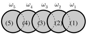
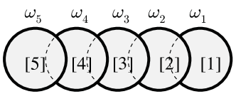
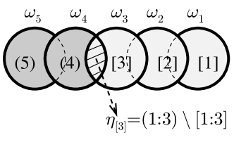
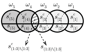
Figure 5.2.1: The topology of $n=5$ factor index sets $\omega_{1},\ldots,\omega_{n}$ in (5.1.5), together with the operator index set $\mathcal{S}\subseteq\Omega$ in (5.1.8)

5.2.1 Separated indices of factors

5.2.1.1 No-longer-needed (NLN) algorithm

In CI structure, the aim is to divide the universe $\Omega$ into $n$ partitions (or “bins”) of variables. From (5.1.5), we can define two ways to partition $\Omega$, one backward and one forward, as follows:

$$\Omega = \omega_{1}\cup\cdots\cup\omega_{n}$$

$$= \{\boldsymbol{(1)},\ldots,\boldsymbol{(n)}\}$$

$$= \{\boldsymbol{[1]},\ldots,\boldsymbol{[n]}\}$$

where the NLN index sets $\boldsymbol{[i]}$ (Definition 5.2.1) and the FA index set $\boldsymbol{(i)}$ (Definition 5.2.2) are (possibly empty) subsets of $\Omega$, $i=1,\ldots,n$.

Because $\omega_{i}$ might be overlapped with each other, let us denote:

$$\boldsymbol{\omega}_{i:j}\triangleq\omega_{i}\cup\cdots\cup\omega_{j},\ 1\leq i\leq j\leq n.$$

Then the task is to extract $\boldsymbol{(i)}$ and $\boldsymbol{[i]}$ from $\{\omega_{1},\ldots,\omega_{n}\}$, as follows:

Definition 5.2.1.

(No-longer-needed (NLN) indices)
Let us consider $n$ backward nested sets $\omega_{n}=\boldsymbol{\omega}{}_{n:n}\subseteq\boldsymbol{\omega}_{n-1:n}\subseteq\cdots\subseteq\boldsymbol{\omega}_{1:n}=\Omega$ and extract $n$ partitions of $\Omega$, as follows: $\boldsymbol{[i]}=\boldsymbol{\omega}_{i:n}\backslash\boldsymbol{\omega}_{i+1:n}$, $\forall i\in\{1,\ldots,n\}$ (upper-right schematic in Fig. 5.2.1). We call $\boldsymbol{[i]}$ a set of no-longer-needed indices for set $\omega_{i}$, $i=n,\ldots,1$, owing to the fact that $\boldsymbol{[i]}\subseteq\omega_{i}$ and $\boldsymbol{[i]}\not\subset\boldsymbol{\omega}_{i+1:n}$.

  

Definition 5.2.2.

(First-appearance (FA) indices)
Let us consider $n$ forward nested sets $\omega_{1}=\boldsymbol{\omega}_{1:1}\subseteq\cdots\subseteq\boldsymbol{\omega}_{1:n-1}\subseteq\boldsymbol{\omega}_{1:n}=\Omega$, we can also extract other $n$ partitions of $\Omega$, as follows: $\boldsymbol{(i)}=\boldsymbol{\omega}_{1:i+1}\backslash\boldsymbol{\omega}_{1:i}$, $\forall i\in\{1,\ldots,n\}$ (upper-left schematic in Fig. 5.2.1). We call $\boldsymbol{(i)}$ a set of first-appearance indices at point $i=1,\ldots,n$, owing to the fact that $\boldsymbol{(i)}\subseteq\omega_{i}$ and $\boldsymbol{(i)}\not\subset\boldsymbol{\omega}_{1:i-1}$.

For deriving a sequence of $\boldsymbol{[i]}$ and $\boldsymbol{(i)}$, induced by (5.2.1.1), we can directly apply the Definition 5.2.1, 5.2.2, respectively. However, an extraction algorithm can also be designed, as presented below.

Firstly, let us design an $m\times n$ occupancy matrix $\Omega_{m\times n}$ for the universe $\Omega=\omega_{1}\cup\cdots\cup\omega_{n}$, as follows:

$$\begin{array}[]{c}\begin{array}[]{c}(\Omega_{m\times n})\end{array}\\ \begin{array}[]{c}m\\ \vdots\\ 1\end{array}\end{array}\begin{array}[]{c}\begin{array}[]{ccc}\omega_{n}\ldots&\omega_{i}\ldots&\omega_{1}\end{array}\\ \left[\begin{array}[]{ccc}\delta_{m,n}&\delta_{m,i}&\delta_{m,1}\\ \vdots&\vdots&\vdots\\ \delta_{1,n}&\delta_{1,i}&\delta_{1,1}\end{array}\right]\end{array}$$ (5.2.2)

where:

- the whole matrix is, for convenience, labelled $(\Omega_{m\times n})$;

- $n$ columns, from the first to the last column, are labelled by $\omega_{n},\ldots,\omega_{1}$, respectively (i.e in the reverse order);

- $m$ rows, from the first to the last row, are labelled by variable indices $k=m,\ldots,1$, respectively (i.e in the reverse order) in the universe $\Omega$;

- $\delta_{k,i}$ denotes binary indicator (i.e. a Kronecker function): $\delta_{k,i}=1$ if $k\in\omega_{i}$, and $\delta_{k,i}=0$ otherwise, $1\leq k\leq m$, $1\leq i\leq n$.

The reason for the reverse order in labelling is to preserve the band-diagonal property for the case of the Markov chain, as illustrated in Example 5.2.5, what follows shortly.

From the occupancy matrix (5.2.2), we can see that the necessary and sufficient condition for $k\in\boldsymbol{[i]}=\boldsymbol{\omega}_{i:n}\backslash\boldsymbol{\omega}_{i+1:n}$, is that - in row $k$ - value $1$ appears at column $i$ and value $0$ appears at all columns $\{i+1,\ldots,n\}$ , i.e. $\delta_{k,i}=1$ and $\delta_{k,j}=0$, with $j=i+1,\ldots,n$ . Hence, the set $\boldsymbol{[i]}$, $i=1,\ldots,n$, consists of all those row indices containing value $1$ at column $\omega_{i}$.

Similarly, we can take the indices of rows for which the first-$1$ from the right occurs at column $i$, as constituting the $i$th first-appearance (FA) set, $\boldsymbol{(i)}$.

We can design an algorithm for construction of the $n$ no-longer-needed (NLN) sets, $\boldsymbol{[i]}$, as illustrated in Algorithm 5.1.

Initialization:

- Constructing occupancy matrix $\Omega_{m\times n}$ (5.2.2) for $\omega_{1},\ldots,\omega_{n}$.

- Initialize $\boldsymbol{[i]}=\emptyset$, $\forall i=1,2,\ldots,n$

- Initialize $n+1$ counter matrices, $C_{n+1}=\Omega_{m\times n}$ and $C_{i}=\emptyset$, $\forall i=1,2,\ldots,n$

Recursion:

For each $i=n,\ldots,1$ (i.e. from the first to the last column), do: { $C_{i}\leftarrow C_{i+1}$;

For each row $k$ at column $\omega_{i}$ in matrix $C_{i}$, do: {

if $\delta_{k,i}=1$, do: {

- add value $k$ to the set $\boldsymbol{[i]}$

- delete row $k$ from $C_{i}$

}} Stop if $C_{i}=\emptyset$ }

Return: the sets $\boldsymbol{[i]}$, $i=1,2,\ldots,n$

Complexity: $O(m)\leq O(m(n-i_{c}+1))\leq O(mn)$ of Boolean comparison $\delta_{k,i}$ for $m$ rows and $(n-i_{c}+1)$ columns, until stopping at column $\omega_{i_{c}}$, $1\leq i_{c}\leq n$.

Algorithm 5.1 No-longer-needed (NLN) algorithm

The NLN algorithm (Algorithm 5.1) for sets $\boldsymbol{(i)}$ are can be designed similarly, but taking the the values $i=1,\ldots,n$ (i.e. from the last to the first column).

Note that, the NLN algorithm (Algorithm 5.1) is merely a straightforward design from Definition 5.2.1, without considering any sorting technique. Hence, the computational complexity of the NLN algorithm is not optimized and ranges from lower bound $O(m)$ to upper bound $O(mn)$. If sorting techniques are also applied, we can conjecture that the expectation of NLN’s complexity will be close to $m$.

In the probability context, the output of NLN algorithm (Algorithm 5.1) exactly corresponds to a valid probability chain rule factorization for joint distribution, as explained in Section 5.5.3.

Remark 5.2.3.

The two-directional topological NLN partition $\boldsymbol{[i]}$ and FA partition $\boldsymbol{(i)}$ of the universe index set $\Omega$, defined in (5.2.1.1), are novel. Likewise, the NLN algorithm, whose purpose is to identify NLN and FA partitions of $\Omega$ induced by the factor index set algebra (5.1.5), has not been proposed elsewhere in the literature. These partitions will be important for our proposal to reduce computational load in evaluating objective functions, later in the thesis.

A related algorithm to the NLN algorithm is the topological sorting algorithm [Cormen et al. (2001)], which returns a topological ordering of a directed acyclic graph (DAG) (i.e. a valid probability chain rule order). The key difference is that, the topological sort permutes the order of factors $\omega_{\pi(1)},\ldots,\omega_{\pi(n)}$ until a valid chain rule order is achieved, while NLN algorithm maintains the same order of factors $\omega_{1},\ldots,\omega_{n}$, but identifies a new probability chain rule order via $\boldsymbol{[i]},\ i=1,2,\ldots,n$, extracted from $\omega_{1},\ldots,\omega_{n}$ (see Section 5.5.3)

Example 5.2.4.

Let us assume that $m=5$, $n=4$ and $\omega_{4}=\{5,3,1\}$, $\omega_{3}=\{4,3\}$, $\omega_{2}=\{3,2\}$, $\omega_{1}=\{2,1\}$. Then, we can write down the occupancy matrix, as follows:

$$\begin{array}[]{c}(\Omega_{5\times 4})\\ 5\\ 4\\ 3\\ 2\\ 1\end{array}\left[\begin{array}[]{cccc}\omega_{4}&\omega_{3}&\omega_{2}&\omega_{1}\\ ([1])&0&0&0\\ 0&([1])&0&0\\ {}[1]&1&(1)&0\\ 0&0&[1]&(1)\\ {}[1]&0&0&(1)\end{array}\right]$$ (5.2.3)

where $[\cdot]$, $(\cdot)$ and $([\cdot])$ indicating elements belonging to no-longer-needed (NLN) indices $\boldsymbol{[i]}$, first-appearance (FA) indices $\boldsymbol{(i)}$ and both of these sets, respectively.

For illustration, the counter matrices, $C_{i}$, for NLN algorithm sequentially are: $C_{5}=\Omega_{5\times 4}$ and:

$$\begin{array}[]{c}(C_{4})\\ -\\ 4\\ -\\ 2\\ -\end{array}\left[\begin{array}[]{cccc}\omega_{4}&\omega_{3}&\omega_{2}&\omega_{1}\\ -&-&-&-\\ 0&[1]&0&0\\ -&-&-&-\\ 0&0&1&1\\ -&-&-&-\end{array}\right],\ \begin{array}[]{c}(C_{3})\\ -\\ -\\ -\\ 2\\ -\end{array}\left[\begin{array}[]{cccc}\omega_{4}&\omega_{3}&\omega_{2}&\omega_{1}\\ -&-&-&-\\ -&-&-&-\\ -&-&-&-\\ 0&0&[1]&1\\ -&-&-&-\end{array}\right],\ \begin{array}[]{c}(C_{2})\\ -\\ -\\ -\\ -\\ -\end{array}\left[\begin{array}[]{cccc}\omega_{4}&\omega_{3}&\omega_{2}&\omega_{1}\\ -&-&-&-\\ -&-&-&-\\ -&-&-&-\\ -&-&-&-\\ -&-&-&-\end{array}\right]$$

Hence, the NLN algorithm stops at $C_{2}=\emptyset$ and returns the no-longer-needed (NLN) sets, as follows: $\boldsymbol{[4]}=\omega_{4}=\{5,3,1\}$, $\boldsymbol{[3]}=\{4\}$, $\boldsymbol{[2]}=\{2\}$ and $\boldsymbol{[1]}=\emptyset$.

  

Example 5.2.5.

For later use, let us consider a canonical (and simpler) example for a first-order Markov chain, with $m=5$, $n=4$, i.e. we have $\omega_{4}=\{5,4\}$, $\omega_{3}=\{4,3\}$, $\omega_{2}=\{3,2\}$, $\omega_{1}=\{2,1\}$. Then, similarly to Example 5.2.4, we can write down the occupancy matrix, as follows:

$$\begin{array}[]{c}(\Omega_{5\times 4})\\ 5\\ 4\\ 3\\ 2\\ 1\end{array}\left[\begin{array}[]{cccc}\omega_{4}&\omega_{3}&\omega_{2}&\omega_{1}\\ ([1])&0&0&0\\ {}[1]&(1)&0&0\\ 0&[1]&(1)&0\\ 0&0&[1]&(1)\\ 0&0&0&([1])\end{array}\right]$$ (5.2.4)

where $[\cdot]$, $(\cdot)$ and $([\cdot])$ indicating elements belonging to no-longer-needed (NLN) indices $\boldsymbol{[i]}$, first-appearance (FA) indices $\boldsymbol{(i)}$ and both of these sets, respectively.

For illustration, the counter matrices, $C_{i}$, for NLN algorithm sequentially are: $C_{5}=\Omega_{5\times 4}$ and:

$$\begin{array}[]{c}(C_{4})\\ -\\ -\\ 3\\ 2\\ 1\end{array}\left[\begin{array}[]{cccc}\omega_{4}&\omega_{3}&\omega_{2}&\omega_{1}\\ -&-&-&-\\ -&-&-&-\\ 0&[1]&1&0\\ 0&0&1&1\\ 0&0&0&1\end{array}\right],\ \begin{array}[]{c}(C_{3})\\ -\\ -\\ -\\ 2\\ 1\end{array}\left[\begin{array}[]{cccc}\omega_{4}&\omega_{3}&\omega_{2}&\omega_{1}\\ -&-&-&-\\ -&-&-&-\\ -&-&-&-\\ 0&0&[1]&1\\ 0&0&0&1\end{array}\right],\ \begin{array}[]{c}(C_{2})\\ -\\ -\\ -\\ -\\ 1\end{array}\left[\begin{array}[]{cccc}\omega_{4}&\omega_{3}&\omega_{2}&\omega_{1}\\ -&-&-&-\\ -&-&-&-\\ -&-&-&-\\ -&-&-&-\\ 0&0&0&[1]\end{array}\right]$$

Hence, the NLN algorithm stops at $C_{1}=\emptyset$ and returns the no-longer-needed (NLN) sets, as follows: $\boldsymbol{[4]}=\omega_{4}=\{5,4\}$, $\boldsymbol{[3]}=\{3\}$, $\boldsymbol{[2]}=\{2\}$ and $\boldsymbol{[1]}=\{1\}$.

5.2.1.2 Ternary partition and in-process factors

.Let us denote $\boldsymbol{[i:j]}=\{\boldsymbol{[i]},\ldots,\boldsymbol{[j]}\}$, $\boldsymbol{(i:j)}=\{\boldsymbol{(i)},\ldots,\boldsymbol{(j)}\}$, $1\leq i\leq j\leq n$. Then we have the following proposition:

Proposition 5.2.6.

(Ternary partition)
For any $i=1,\ldots,n$, we can divide $\Omega=\boldsymbol{\omega}_{i+1:n}\cup\boldsymbol{\omega}_{1:i}$ into ternary partitions:

$$\Omega=\{\boldsymbol{(i+1:n)},\eta_{[i]},\boldsymbol{[1:i]}\}$$ (5.2.5)

in which the (possibly empty) set $\eta_{[i]}$ is called the set of common indices (Fig. 5.2.1):

$$\eta_{[i]}\triangleq\boldsymbol{\omega}_{i+1:n}\cap\boldsymbol{\omega}_{1:i}=\boldsymbol{(1:i)}\backslash\boldsymbol{[1:i]}$$ (5.2.6)

Also, the left and right complement sets in (5.2.5), respectively, are:

$$\boldsymbol{(i+1:n)} = \boldsymbol{\omega}_{i+1:n}\backslash\eta_{[i]}$$ (5.2.7)

$$\boldsymbol{[1:i]} = \boldsymbol{\omega}_{1:i}\backslash\eta_{[i]}$$ (5.2.8)

Proof.

Firstly, let us recall the notation of the intersection part: $\eta_{[i]}\triangleq\boldsymbol{\omega}_{i+1:n}\cap\boldsymbol{\omega}_{i}$, $i=1,\ldots,n$. Then, the proof is carried out via following three steps:
Step 1: For proof of (5.2.8): by Definition 5.2.1 for NLN indices, we have $\boldsymbol{[j]}\triangleq\boldsymbol{\omega}_{j:n}\backslash\boldsymbol{\omega}_{j+1:n}$, hence:

$$\boldsymbol{[i+1:n]}=\cup_{j=i+1}^{n}\boldsymbol{[j]}=\cup_{j=i+1}^{n}\{\boldsymbol{\omega}_{j:n}\backslash\boldsymbol{\omega}_{j+1:n}\}=\boldsymbol{\omega}_{i+1:n}$$

where the last equality was derived via a sequence of merging, e.g. $\{\boldsymbol{\omega}_{1:n}\backslash\boldsymbol{\omega}_{2:n}\}\cup\{\boldsymbol{\omega}_{2:n}\backslash\boldsymbol{\omega}_{3:n}\}=\boldsymbol{\omega}_{1:n}$ . Then, since $\boldsymbol{[i+1:n]}=\boldsymbol{\omega}_{i+1:n}$, we also have:

$$\boldsymbol{[1:i]}=\Omega\backslash\boldsymbol{[i+1:n]}=\Omega\backslash\boldsymbol{\omega}_{i+1:n}=\boldsymbol{\omega}_{1:i}\backslash\eta_{[i]}$$

where the last equality is a consequence of two basic set operators, intersection and union, i.e.: $\eta_{[i]}\triangleq\boldsymbol{\omega}_{i+1:n}\cap\boldsymbol{\omega}_{1:i}$ and $\Omega=\boldsymbol{\omega}_{i+1:n}\cup\boldsymbol{\omega}_{1:i}$, respectively.
Step 2: Similarly, for the proof of (5.2.7): by Definition 5.2.2 of FA indices, we have:

$$\boldsymbol{(1:i)} = \cup_{j=1}^{i}\boldsymbol{(j)}=\cup_{j=1}^{i}\{\boldsymbol{\omega}_{1:j+1}\backslash\boldsymbol{\omega}_{1:j}\}=\boldsymbol{\omega}_{1:i}$$

$$\Rightarrow\boldsymbol{(i+1:n)} = \Omega\backslash\boldsymbol{(1:i)}=\Omega\backslash\boldsymbol{\omega}_{1:i}=\boldsymbol{\omega}_{i+1:n}\backslash\eta_{[i]}$$

Step 3: From above proofs of (5.2.7) and (5.2.8), the ternary partitions for $\Omega$ in (5.2.5) can be proved as follows:

$$\Omega=\boldsymbol{\omega}_{i+1:n}\cup\boldsymbol{\omega}_{1:i} = \{\boldsymbol{\omega}_{i+1:n}\backslash\eta_{[i]},\eta_{[i]},\boldsymbol{\omega}_{1:i}\backslash\eta_{[i]}\}$$

$$= \{\boldsymbol{(i+1:n)},\eta_{[i]},\boldsymbol{[1:i]}\},\ i=1,\ldots,n$$

∎

Proposition 5.2.6 also motivates a definition for in-process variable indices, as follows. These will be important in recursive computation later:

Proposition 5.2.7.

(In-process indices)
In-process indices are defined as tri-partitioned index-sets, $\mathcal{A}_{i}$, associated with the ternary partition $\Omega$ in (5.2.5), as follows:

$$\mathcal{A}_{i} \triangleq \{\boldsymbol{(i+1)},\eta_{[i]},\boldsymbol{[i]}\}$$

$$= \mbox{$\omega_{i+1}\cup\omega_{i}$},\ i=1,\ldots,n$$

Then, from (5.2.5) and (5.2.7), we have:

$$\Omega=\mathcal{A}_{1}\cup\cdots\cup\mathcal{A}_{n}$$ (5.2.10)

Proof.

From Definition 5.2.1, 5.2.2 and (5.2.6), we have:

$$\mathcal{A}_{i} \triangleq \{\boldsymbol{(i+1)},\eta_{[i]},\boldsymbol{[i]}\}$$

$$= \{\boldsymbol{\omega}_{1:i+1}\backslash\boldsymbol{\omega}_{1:i},\boldsymbol{\omega}_{i+1:n}\cap\boldsymbol{\omega}_{1:i},\boldsymbol{\omega}_{i:n}\backslash\boldsymbol{\omega}_{i+1:n}\}$$

$$= \mbox{$\omega_{i+1}\cup\omega_{i}$},\ i=1,\ldots,n$$

as illustrated in lower-left schematic in Fig. 5.2.1 for the case $i=3$. ∎

From (5.2.5), we can see that, in general, the in-process index sets $\mathcal{A}_{i}$ in (5.2.10) are not separated partitions of $\Omega$. Note that, since $\eta_{[i]}=\boldsymbol{\omega}_{i+1:n}\cap\boldsymbol{\omega}_{1:i}$, it might be empty (e.g. when $\omega_{1},\ldots,\omega_{n}$ are separated partitions of $\Omega=\{\omega_{1},\ldots,\omega_{n}\}$). In contrast, the set $\mathcal{A}_{i}$, defined by (5.2.7), cannot be empty, since $\omega_{i}\neq\emptyset$, $i=1,\ldots,n$, by definition (Section 5.1.1). Moreover, different from union of tri-partitioned sets $\mathcal{A}_{i}$ in (5.2.10), the union of common sets $\eta_{[1]}\cup\cdots\cup\eta_{[n]}$ is not necessary equal to $\Omega$.

For these reasons, we prefer to compute the operators in (5.1.10) via tri-partitioned sets $\mathcal{A}_{i}$ instead of common sets $\eta_{[i]}$.

5.2.2 Separated indices of operators

5.2.2.1 Binary partition

From (5.1.8) and (5.2.1.1), we can distribute the single operator index set $\mathcal{S}$ and objective index set $\mathcal{S}^{c}$ across two $n$ alternative partitions, as follows:

$$\mathcal{S} = \{s_{\boldsymbol{(1)}},\ldots,s_{\boldsymbol{(n)}}\}$$

$$= \{s_{\boldsymbol{[1]}},\ldots,s_{\boldsymbol{[n]}}\}$$

$$\mathcal{S}^{c} = \{s_{\boldsymbol{(1)}}^{c},\ldots,s_{\boldsymbol{(n)}}^{c}\}$$

$$= \{s_{\boldsymbol{[1]}}^{c},\ldots,s_{\boldsymbol{[n]}}^{c}\}$$

where, $i=1,\ldots,n$, and:

$$s_{\boldsymbol{(i)}} \triangleq \mathcal{S}\cap\boldsymbol{(i)}$$ (5.2.11)

$$s_{\boldsymbol{[i]}} \triangleq \mathcal{S}\cap\boldsymbol{[i]}$$

$$s_{\boldsymbol{(1)}}^{c} \triangleq \boldsymbol{(i)}\backslash s_{\boldsymbol{(i)}}$$

$$s_{\boldsymbol{[1]}}^{c} \triangleq \boldsymbol{[i]}\backslash s_{\boldsymbol{[i]}}$$

as illustrated in lower-right schematic in Fig. 5.2.1.

5.2.2.2 Ternary partition and in-process operators

Proceeding as in Section 5.2.1.2, then, from (5.1.8) and (5.2.5), the ternary partitions of $\mathcal{S}$ and $\mathcal{S}^{c}$ can be defined, respectively, as follows:

$$\mathcal{S} = \{s_{\boldsymbol{(i+1:n)}},s_{\eta_{[i]}},s_{\boldsymbol{[i]}}\}$$ (5.2.12)

$$\mathcal{S}^{c} = \{s_{\boldsymbol{(i+1:n)}}^{c},s_{\eta_{[i]}}^{c},s_{\boldsymbol{[i]}}^{c}\},$$

where, $i=1,\ldots,n$, and:

$$s_{\eta_{[i]}} \triangleq \mathcal{S}\cap\eta_{[i]}$$ (5.2.13)

$$s_{\eta_{[i]}}^{c} \triangleq \eta_{[i]}\backslash s_{\eta_{[i]}}$$

as illustrated in lower-right schematic in Fig. 5.2.1.

5.2.2.3 Non-overflowed (NOF) condition

For sequential objective functions (5.1.11), let us consider a sequence of subsets $\mathcal{S}_{j}$, such that $\mathcal{S}=\mathcal{S}_{1}\cup\cdots\cup\mathcal{S}_{\kappa},$ and $\mathcal{S}_{j}\subset\mathcal{S}\subseteq\Omega$, $j=1,\ldots,\kappa$. Denoting objective set $\bar{\mathcal{S}}_{j}\neq\emptyset$ as complement of $\mathcal{S}_{j}$ in $\mathcal{S}$, we will consider a special case of $\bar{\mathcal{S}}_{j}$, as follows:

Definition 5.2.8.

(Non-overflowed (NOF) set and NOF condition)
A set $\bar{\mathcal{S}}_{j}$, with $j\in\{1,\ldots,\kappa\}$, is called non-overflowed (NOF) set if the following NOF condition is satisfied:

$$\exists i\in\{1,\ldots,n\}:\ \bar{\mathcal{S}}_{j}\subseteq\mathcal{S}_{\mathcal{A}_{i}}\triangleq\{s_{\boldsymbol{(i+1)}},s_{\eta_{[i]}},s_{\boldsymbol{[i]}}\}\subseteq\mathcal{S},\ j\in\{1,\ldots,\kappa\}$$ (5.2.14)

Otherwise, $\bar{\mathcal{S}}_{j}$ is called an overflowed set.

The meaning of the name is as follows: given a tri-partitioned set $\mathcal{A}_{i}$ (5.2.7) being in process/memory at point $i\in\{1,\ldots,n\}$, the objective set $\bar{\mathcal{S}}_{j}\subseteq\mathcal{S}_{\mathcal{A}_{i}}$ can be extracted within current process/memory $\mathcal{A}_{i}$ and does not cause extra/overflowed work.

For later use, let us also define the complement of $\bar{\mathcal{S}}_{j}$ in $\mathcal{S}_{\mathcal{A}_{i}}$, as follows:

$$\mathcal{S}_{\mathcal{A}_{i}}^{\backslash j} \triangleq \mathcal{S}_{\mathcal{A}_{i}}\backslash\bar{\mathcal{S}}_{j}$$

$$= \mathcal{S}_{\mathcal{A}_{i}}\cap S_{j}$$

$$= \{s_{\boldsymbol{(i+1)}}^{\backslash j},s_{\eta_{[i]}}^{\backslash j},s_{\boldsymbol{[i]}}^{\backslash j}\}$$

in which the intersection is carried out element-wise. Finally, let us consider the most special case of non-overflowed set, which is scalar set, as follows:

Proposition 5.2.9.

(Objective scalar sets)
The singleton sets, $\bar{\mathcal{S}}_{j}=\{j\}\in\mathcal{S}=\Omega$, $j=1,\ldots,\kappa$, where $\kappa=m$, are non-overflowed sets.

Proof.

Firstly, by definition of $\omega_{i}$, there always exists $i\in\{1,\ldots,n\}$ such that:

$$\bar{\mathcal{S}}_{j}=\{j\}\in\omega_{i+1}\cup\omega_{i}=\mathcal{A}_{i},\ \exists i\in\{1,\ldots,n\},\forall j\in\{1,\ldots,\kappa\}$$ (5.2.16)

where the last equality is owing to (5.2.7).

Secondly, owing to the assumption $\kappa=m$, we have $\mathcal{S}=\cup_{j=1}^{m}\bar{\mathcal{S}}_{j}=\cup_{j=1}^{m}\{j\}=\Omega$.

Thirdly, by definitions in (5.2.7,5.2.14), we have:

$$\mathcal{A}_{i}=\{\boldsymbol{(i+1)},\eta_{[i]},\boldsymbol{[i]}\}=\{s_{\boldsymbol{(i+1)}},s_{\eta_{[i]}},s_{\boldsymbol{[i]}}\}=\mathcal{S}_{\mathcal{A}_{i}},\ \forall i\in\{1,\ldots,m\}$$ (5.2.17)

owing to $\mathcal{S}=\Omega$ above and (5.2.11-5.2.13).

Finally, from (5.2.16) and (5.2.17), we have $\bar{\mathcal{S}}_{j}\subseteq\mathcal{S}_{\mathcal{A}_{i}}\subseteq\mathcal{S}=\Omega,\ \exists i\in\{1,\ldots,n\},$ which satisfies the NOF condition (5.2.14), $\forall j\in\{1,\ldots,\kappa\}$ and $\kappa=m$. ∎

Note that, the assumption $\kappa=m$ is useful in Proposition 5.2.9, since it facilitate the verification of (5.2.17) in the proof. In Bayesian analysis, the assumption $\kappa=m$ is often valid when a sequence of all marginals needs to be computed (e.g for computing minimum risk estimator computation (4.3.8)). For the case $\kappa=\kappa_{0}<m$ but $\kappa_{0}$ is close enough to $m$, we may consider the augmented case $\kappa=m$, i.e. $S=\Omega$, like above, but only return the results corresponding to the NOF sets $\bar{\mathcal{S}}_{j}$, $j\in\Omega\backslash\{\kappa_{0}+1,\ldots,m\}$.

5.3 Generalized distributive law (GDL)

In this section, let us recall the abstract algebra and exploit the distributive law associated with ring theory. For clarity, let us firstly emphasize that ring theory can be applied feasibly to a set of either variables or functions, i.e.:

- In abstract algebra [Hazewinkel (1995)] and in graph theory [Aji and McEliece (2000)], the standard definitions of a group and a ring begin with a standard set $\mathcal{R}$, associated with binary operators.

- Because the point-wise value of any function $g:\mathcal{X}\rightarrow\mathcal{R}$ can be considered as a set $\mathcal{R}$, for each $x\in\mathcal{X}$, the above standard definition of group and ring can be applied to a set of function values $g(x)$ in the same way as standard set $\mathcal{R}$ [Gillman and Jerison (1960)]. Hence, the GDL in ring theory can be applied directly to all functions $g_{i}$ in (5.1.7) [Gondran and Minoux (2008)], without the need of re-definition.

Without loss of generality, let us avoid the former approach, which is used in [Aji and McEliece (2000)], and begin with latter approach, i.e. abstract algebra for a set of functions. As shown below, the latter is more general and actually an important step in algorithm design, because the set of functions will clarify the number of operators required in computing the objective functions (5.1.7).

5.3.1 Abstract algebra

Let us consider a set $\mathcal{R}^{\mathcal{X}_{\Omega}}$ of functions $g:\mathcal{X}_{\Omega}\rightarrow\mathcal{R}$. Then we have following definitions:

Definition 5.3.1.

(Commutative semigroup of functions)
A commutative semigroup $(\mathcal{R}^{\mathcal{X}_{\Omega}},\boxtimes)$ is a set $\mathcal{R}^{\mathcal{X}_{\Omega}}$ of $\mathcal{R}$-value functions on domain $\mathcal{X}_{\Omega}$, associated with closure binary operator $\boxtimes:\mathcal{R}^{\mathcal{X}_{\Omega}}\times\mathcal{R}^{\mathcal{X}_{\Omega}}\rightarrow\mathcal{R}^{\mathcal{X}_{\Omega}}:f(\mathbf{x})\boxtimes g(\mathbf{x})\rightarrow q(\mathbf{x})\triangleq(f\boxtimes g)(\mathbf{x})$, such that following two properties hold:
Associative Law: $f\boxtimes(g\boxtimes h)=(f\boxtimes g)\boxtimes h$
Commutative Law: $f\boxtimes g=g\boxtimes f$
for any $\mathbf{x}\in\mathcal{X}_{\Omega}$ and $f,g,h,q\in\mathcal{R}^{\mathcal{X}_{\Omega}}$.

  

Definition 5.3.2.

(Commutative pre-semiring of functions)
A commutative pre-semiring $(\mathcal{R}^{\mathcal{X}_{\Omega}},\boxplus,\odot)$ is a set $\mathcal{R}^{\mathcal{X}_{\Omega}}$ of $\mathcal{R}$-value functions on domain $\mathcal{X}_{\Omega}$, associated with two commutative semigroups $(\mathcal{R}^{\mathcal{X}_{\Omega}},\boxplus)$ and $(\mathcal{R}^{\mathcal{X}_{\Omega}},\odot)$, such that following two properties hold:
Priority order of operation: $f\odot g\boxplus h=(f\odot g)\boxplus h\neq f\odot(g\boxplus h)$
Distributive law: $f\odot(g\boxplus h)=(f\odot g)\boxplus(f\odot h)$
for $f,g,h\in\mathcal{R}^{\mathcal{X}_{\Omega}}$.

Note that, in abstract algebra, the above concept of pre-semiring (Definition 5.3.2) and traditional semiring, which additionally requires the existence of two identity elements (one for $\boxplus$ and one for $\odot$), are not equivalent [Hazewinkel (1995)]. In graph theory, the definition of semiring together with the identity elements is widely used in many papers [Fettweis and Meyr (1990); Aji and McEliece (2000); Ilic et al. (2011)]. Therefore, we use the name “pre-semiring”, as proposed in [Minoux (2001); Gondran and Minoux (2008)], and consider semiring as a special case of a pre-semiring. In contrast to a semiring structure, the pre-semiring is more relaxed and does not require the existence of the identity elements.

5.3.2 Ring-sum and ring-product

Let us denote $\mathcal{X}_{\omega}\subseteq\mathcal{X}_{\Omega}$ as a subspace of $\mathcal{X}_{\Omega}$, with $\omega\subseteq\Omega$, as in Section 5.1.1. By generalizing the range from the set of real number $\mathbb{R}$ to an arbitrary set $\mathcal{R}$, the functions in our model (5.1.7) become $g_{i}:\ \mathcal{X}_{\omega_{i}}\rightarrow\mathcal{R}$. Moreover, it is feasible to recognize that $g_{i}\in\mathcal{R}^{\mathcal{X}_{\Omega}}$, since $\mathcal{R}^{\mathcal{X}_{\omega_{i}}}\subseteq\mathcal{R}^{\mathcal{X}_{\Omega}}$. Consequently, we can apply the abstract algebra above in the pre-semiring $(\mathcal{R}^{\mathcal{X}_{\Omega}},\boxplus,\odot)$ to all functions, $g_{i}$. Note that, by the above definitions from ring theory, the closure property of any operators $\boxplus$, $\odot$ applied to $g_{i}$ is guaranteed within the space $\mathcal{R}^{\mathcal{X}_{\Omega}}$, but not guaranteed within its sub-space $\mathcal{R}^{\mathcal{X}_{\omega_{i}}}$.

For computation of our specific model (5.1.7), we need, however, to define some specific ring-sum and ring-product operators properly. These definitions also clarify the number of required operators in the sequel.

Definition 5.3.3.

(Ring-sum)
Let us consider $g\in\mathcal{R}^{\mathcal{X}_{\omega}}$. Given $i\in\omega\subseteq\Omega$ and $\mathcal{X}\triangleq\{\bar{x}_{1},\ldots,\bar{x}_{M}\}$, then the $i$th ring-sum is defined as:
$\underset{x_{i}}{\boxplus}g(\mathbf{x}_{\omega})=g_{\bar{x}_{1}}\boxplus g_{\bar{x}_{2}}\boxplus\cdots\boxplus g_{\bar{x}_{M}}$
where $g_{\bar{x}_{j}}\triangleq g(x_{i}=\bar{x}_{j},\mathbf{x}_{\omega\backslash i})$ with $x_{i}\in\mathcal{X}$, $j=1,\ldots,M$ and, as before, $M\triangleq|\mathcal{X}|$ (5.1.3)
In this way, we can define a projection function: $\underset{x_{S}}{\boxplus}:\ \mathcal{R}^{\mathcal{X}_{\omega}}\rightarrow\mathcal{R}^{\mathcal{X}_{\omega\backslash S}}$, $\forall\mathcal{S}=\{s_{1},\ldots,s_{|\mathcal{S}|}\}\subseteq\omega$, as follows:

$$\underset{\mathbf{x}_{\mathcal{S}}}{\boxplus}g(\mathbf{x}_{\omega})=\underset{x_{s_{|\mathcal{S}|}}}{\boxplus}\cdots\underset{x_{s_{1}}}{\boxplus}g(\mathbf{x}_{\omega})$$ (5.3.1)

  

Definition 5.3.4.

(Ring-product)
Ring-product is an augmented function: $\odot_{k=i}^{j}:\ \mathcal{R}^{\mathcal{X}_{\omega_{i}}}\times\cdots\times\mathcal{R}^{\mathcal{X}_{\omega_{j}}}\rightarrow\mathcal{R}^{\mathcal{X}_{\omega}}$, where $\omega=\omega_{i}\cup\cdots\cup\omega_{j}$, defined as follows:

$$\odot_{k=i}^{j}g_{k}=g_{j}\odot g_{j-1}\odot\cdots\odot g_{i}$$ (5.3.2)

.

From the definitions above, we will apply the distributive law assumption of pre-semiring in Definition 5.3.2 to our ring-operators, as follows:

Definition 5.3.5.

(Generalized Distributive Law)
By definition of distributive law of pre-semiring in Definition 5.3.2, the generalized distributive law (GDL) for elements can be defined as (from left to right):

$$g_{2}\odot(\underset{x_{S}}{\boxplus}g_{1})=\underset{x_{S}}{\boxplus}(g_{2}\odot g_{1}),\ \forall S\not\subset\omega_{2}$$ (5.3.3)

Then, the reverse flow (from right to left) of (5.3.3) is called the generalized distributive law (GDL) for operators, i.e.:

$$\underset{x_{S}}{\boxplus}(g_{2}\odot g_{1})=g_{2}\odot(\underset{x_{S}}{\boxplus}g_{1}),\ \forall S\not\subset\omega_{2}$$ (5.3.4)

Notice the interesting difference in notation between (5.3.3) and (5.3.4). In “GDL for elements” (5.3.3), it seems that the element $g_{2}$ is distributed across the operators $\boxplus$, while in “GDL for operators” (5.3.4), it looks like the operator $\underset{x_{\mathcal{S}}}{\boxplus}$ is actually the one being distributed.

The “GDL for elements” (5.3.3) - for example, $a_{3}(a_{1}+a_{2})=a_{3}a_{1}+a_{3}a_{2}$ - is more consistent with the traditional distributive law in mathematics textbooks. However, in practice, the “GDL for operators” (5.3.4) - for example, $\sum_{i=1}^{2}(a_{3}a_{i})=a_{3}\left(\sum_{i=1}^{2}a_{i}\right)$ - is more popular and constitutes the definition of the GDL form, e.g. in [Aji and McEliece (2000); Nielsen (2001)]).

In this thesis, the latter is preferred, i.e. “GDL for operators” (5.3.4) will be defined as GDL, although both terms “GDL for elements” and “GDL for operators” are obviously equivalent.

5.3.3 Computational reduction via the GDL

Let us investigate the computational load below by counting the number of operators $\boxplus$ and $\odot$ involved in the ring-sum (5.3.1), ring-product (5.3.2) and GDL (5.3.4).

Intuitively, the computational reduction, from left hand side to right hand side in GDL (5.3.4), comes from the order of the computation of projection (i.e. ring-sum), and augmentation (i.e. ring-product). On the left hand side of (5.3.4), the augmentation is implemented first, followed by projection, while the order is reversed on the right hand side of (5.3.4), i.e projection is implemented first, followed by augmentation. Therefore, the right hand side of (5.3.4) is more efficient because it rules out the nuisance variables $x_{S}$ upfront (i.e. immediately after recognizing that $x_{S}$ is no-longer-needed). In contrast, the left hand side of (5.3.4) is less efficient because the nuisance variables $x_{S}$ are dragged along in the augmentation operator, $g_{2}\odot g_{1}$, and increases the number of computations required for the final result.

In practice, however, this reduction does not always imply an actual reduction in computational load. For example, the quantities involved in the left hand side, $\underset{x_{\mathcal{S}}}{\boxplus}(g_{2}\odot g_{1})$ might be known beforehand and retrieved via table-lookup, while the right hand side quantities might be unknown and hence requires computation. Nevertheless, the general interest is to count the number of operators, because that number is typically assumed to be proportional to computational load in practice.

5.3.3.1 Computational load in ring-sum and ring-product

For convenience, let us denote ${\cal O}[\cdot]$ as a counting procedure returning the order of the number $O_{\boxtimes}$ of operators, $\boxtimes$, applied on function in brackets, $[\cdot]$.

Lemma 5.3.6.

(Computational load in ring-sum and ring-product)
a) The computational load of a ring-sum only depends on dimension $m$ of its function $g\in\mathcal{R}^{\mathcal{X}_{\omega}}$:

$${\cal O}[\underset{\mathbf{x}_{S}}{\boxplus}g(x_{\omega})]=O_{\boxplus}(M^{|\omega|}),\ \forall S\subseteq\omega$$

b) The computational load of ring-product depends on the combined dimension of its two functions:

$${\cal O}[g_{2}\odot g_{1}]=O_{\odot}(M^{|\omega_{1}\cup\omega_{2}|})$$

Proof.

a) For ring-sum, $\underset{x_{i}}{\boxplus}$, in Definition 5.3.3, we need $O_{\boxplus}(M^{|\omega|})$ of operator $\boxplus$. Hence, for $\underset{\mathbf{x}_{\mathcal{S}}}{\boxplus}$, we need $O_{\boxplus}(\sum_{i=|\omega\backslash\mathcal{S}|}^{|\omega|}M^{i})=O_{\boxplus}(M^{|\omega|})$ of operator $\boxplus$.

b) Because the result of binary ring-product $g_{1}(\mathbf{x}_{\omega_{1}})\odot g_{2}(\mathbf{x}_{\omega_{2}})$ is a function with union domains $g(\mathbf{x}_{\omega_{1}\cup\omega_{2}})$, it requires $O(M^{|\omega_{1}\cup\omega_{2}|})$ of operator $\odot$ for computing the $M^{|\omega_{1}\cup\omega_{2}|}$ values of $\mathbf{x}_{\omega_{1}\cup\omega_{2}}$. ∎

5.3.3.2 Computational load in GDL

From Lemma 5.3.6, we can prove the main theorem of this chapter, as follows:

Theorem 5.3.7.

The GDL for operators (5.3.4), if applicable, always reduces the number of operators; i.e.:

$${\cal O}[\underset{x_{S}}{\boxplus}(g_{2}\odot g_{1})]>{\cal O}[g_{2}\odot(\underset{x_{S}}{\boxplus}g_{1})],\ \forall S\not\subset\omega_{2}$$ (5.3.5)

Proof.

From (5.3.4) and Lemma 5.3.6, we have:

$${\cal O}[\underset{x_{\mathcal{S}}}{\boxplus}(g_{2}\odot g_{1})] = {\cal O}[\underset{x_{\mathcal{S}}}{\boxplus}\mathbf{g}_{1:2}]+{\cal O}[g_{2}\odot g_{1}]$$

$$= O_{\boxplus}(M^{|\omega_{1}\cup\omega_{2}|})+O_{\odot}(M^{|\omega_{1}\cup\omega_{2}|})$$

where $\mathbf{g}_{1:2}=g_{2}\odot g_{1}$ is regarded as a point-wise function $\mathbf{g}_{1:2}:\mathcal{X}_{\omega_{1}\cup\omega_{2}}\rightarrow\mathcal{R}$. Likewise, we have:

$${\cal O}[g_{2}\odot(\underset{x_{\mathcal{S}}}{\boxplus}g_{1})] = {\cal O}[\underset{x_{\mathcal{S}}}{\boxplus}g_{1}]+{\cal O}[g_{2}\odot g(\mathbf{x}_{\omega_{1}\backslash\mathcal{S}})]$$

$$= O_{\boxplus}(M^{|\omega_{1}|})+O_{\odot}(M^{|\{\omega_{1}\backslash\mathcal{S}\}\cup\omega_{2}|})$$

Since $|\omega_{1}\cup\omega_{2}|\geq|\omega_{1}|$ and $|\omega_{1}\cup\omega_{2}|\geq|\{\omega_{1}\backslash\mathcal{S}\}\cup\omega_{2}|$, the following non-strict inequality follows:

$${\cal O}[\underset{x_{\mathcal{S}}}{\boxplus}(g_{2}\odot g_{1})]\geq{\cal O}[g_{2}\odot(\underset{x_{\mathcal{S}}}{\boxplus}g_{1})]$$ (5.3.6)

Equality requires both $|\omega_{1}\cup\omega_{2}|=|\omega_{1}|$ and $|\omega_{1}\cup\omega_{2}|=|\{\omega_{1}\backslash\mathcal{S}\}\cup\omega_{2}|$, i.e. $\omega_{2}\subseteq\omega_{1}$ and $\mathcal{S}\subseteq\omega_{1}\cap\omega_{2}$, respectively. However, because the condition for GDL is $S\not\subset\omega_{2}$, or, equivalently $\mathcal{S}\subseteq\omega_{1}\backslash\{\omega_{1}\cap\omega_{2}\}$, the equality in (5.3.6) only happens if the GDL (5.3.4) is invalid. ∎

In Theorem 5.3.7, the GDL is recognized, for the first time, as always reducing the number of operators in any pre-semiring. In the literature, there is no result guaranteeing such a reduction in GDL for all cases in ring theoretic class. The GDL is only explicitly recognized to reduce the number of operators in the trivial cases, such as $a(b+c)=ab+ac$ in mathematical textbooks, and is instead applied to specific models in order to evaluate the reduction on a case-by-case basis [Aji and McEliece (2000); Moon (2005); Cortes et al. (2008); Ilic et al. (2011)].

Moreover, Lemma 5.3.6 provides an explicit formula for counting the number of operators in GDL (5.3.5) via set operators, rather than via a complicated graphical topology in [Aji and McEliece (2000); Moon (2005)].

5.4 GDL for objective functions

In this section, we will propose a novel recursive technique, called forward-backward (FB) recursion, for computing the objective functions in (5.1.9) and (5.1.10). We call this technique FB, owing to its similarity with well known FB algorithm for Hidden Markov Chain in the literature. This similarity will be clarified in Section 6.2.2 of this thesis.

5.4.1 FB recursion for single objective function

After setting up the pre-semiring, $(\mathcal{R}^{X_{m}},\boxplus,\odot)$, our aim is to compute the single objective function (5.1.9):

$$\underset{\mathbf{x}_{\mathcal{S}}}{\boxplus}\mathbf{g}_{1:n}=\underset{\mathbf{x}_{\mathcal{S}}}{\boxplus}(\odot_{i=1}^{n}g_{i})$$ (5.4.1)

with $\mathcal{S}\subseteq\Omega$. From Lemma 5.3.6, we can see that the cost of direct computation on the right hand side of (5.4.1) is exponentially increasing with $m$, i.e. $O(M^{m})$, which is impractical. Because the GDL (5.3.5) always reduces the cost, we will exploit the conditionally independent (CI) structure in (5.4.1) and apply the GDL, as shown below.

5.4.1.1 Binary tree factorization

The joint ring-products (5.1.7) can be written as:

$$\mathbf{g}_{1:n}=\mathbf{g}_{i+1:n}\odot\mathbf{g}_{1:i},\ \ \ i\in\{1,\ldots,n-1\}$$ (5.4.2)

where $\mathbf{g}_{1:i}\triangleq\odot_{j=1}^{i}g_{j}$ and $\mathbf{g}_{i:n}\triangleq\odot_{j=i}^{n}g_{j}$, together with forward and backward recursions:

$$\mathbf{g}_{1:j} = g_{j}\odot\mathbf{g}_{1:j-1},\ \ \ j=2,\ldots,i$$ (5.4.3)

$$\mathbf{g}_{j:n} = g_{j}\odot\mathbf{g}_{j+1:n},\ \ \ j=n-1,\ldots,i+1$$ (5.4.4)

The domains of the functions in (5.4.2-5.4.4) are, respectively:

$$dom(\mathbf{g}_{1:j}) = \{\mathrm{x}_{\eta_{[j]}},\mathbf{x}_{\boldsymbol{[1:j]}}\}$$ (5.4.5)

$$dom(\mathbf{g}_{j+1:n}) = \{\mathbf{x}_{\boldsymbol{(j+1:n)}},\mathrm{x}_{\eta_{[j]}}\}$$

$$dom(\mathbf{g}_{1:n})=\mathbf{x}_{\Omega} = \{\mathbf{x}_{\boldsymbol{(j+1:n)}},\mathrm{x}_{\eta_{[j]}},\mathbf{x}_{\boldsymbol{[1:j]}}\}$$

using the notation defined in Proposition 5.2.6. Then, we will see below that operators, $\boxplus$, upon the joint $\mathbf{g}_{1:n}$ can be distributed into the binary tree structure (5.4.2), owing to the GDL-for-operators form (5.3.4).

5.4.1.2 Derivation of the FB recursion

Let us denote $\widehat{\mathbf{g}}_{1:n}\triangleq\underset{\mathbf{x}_{\mathcal{S}}}{\boxplus}\mathbf{g}_{1:n}=g(\mathbf{x}_{S^{c}})$. Owing to the separable domains in (5.4.5), we can apply the GDL (5.3.4) to computation of operator $\underset{\mathbf{x}_{\mathcal{S}}}{\boxplus}$ on (5.4.2), as follows:

$$\widehat{\mathbf{g}}_{1:n}=\underset{\mathrm{x}_{s_{\eta_{[i]}}}}{\boxplus}(\widehat{\mathbf{g}}_{i+1:n}\odot\widehat{\mathbf{g}}_{1:i}),\ \ \ i\in\{1,\ldots,n-1\}$$ (5.4.6)

where $\mbox{$\widehat{\mathbf{g}}_{1:i}$}\triangleq\underset{\mathbf{x}_{s_{\boldsymbol{[1:i]}}}}{\boxplus}\mathbf{g}_{1:i}$ and $\widehat{\mathbf{g}}_{i:n}\triangleq\underset{\mathbf{x}_{s_{\boldsymbol{(i:n)}}}}{\boxplus}\mathbf{g}_{i:n}$ , together with forward and backward recursions:

$$\widehat{\mathbf{g}}_{1:j} =\underset{\mathrm{x}_{s_{\boldsymbol{[j]}}}}{\boxplus} (g_{j}\odot\widehat{\mathbf{g}}_{1:j-1}),\ \ \ j=2,\ldots,i$$ (5.4.7)

$$\widehat{\mathbf{g}}_{j:n} =\underset{\mathrm{x}_{s_{\boldsymbol{(j)}}}}{\boxplus} (g_{j}\odot\widehat{\mathbf{g}}_{j+1:n}),\ \ \ j=n-1,\ldots,i+1$$ (5.4.8)

The domain of functions in (5.4.6-5.4.8) are:

$$dom(\mbox{$\widehat{\mathbf{g}}_{1:j}$}) = \{\mathrm{x}_{\eta_{[j]}},\mathbf{x}_{s_{\boldsymbol{[1:j]}}^{C}}\}$$ (5.4.9)

$$dom(\widehat{\mathbf{g}}_{j+1:n}) = \{\mathbf{x}_{s_{\boldsymbol{(j+1:n)}}^{C}},\mathrm{x}_{\eta_{[j]}}\}$$

$$dom(\widehat{\mathbf{g}}_{1:n})=\mathbf{x}_{\mathcal{S}^{c}} = \{\mathbf{x}_{s_{\boldsymbol{(i+1:n)}}^{C}},\mathrm{x}_{s_{\eta_{[i]}}^{c}},\mathbf{x}_{s_{\boldsymbol{[1:i]}}^{C}}\}$$

Examining (5.4.5) with (5.4.9), we can see that the variable indices in these domains can be feasibly derived via the set algebras in (5.2.5) and (5.2.12), respectively. It is also important to emphasize that, for computing a single objective function, $\widehat{\mathbf{g}}_{1:n}$ in (5.4.6), the value $i\in\{1,\ldots,n-1\}$ can be chosen arbitrarily, since each yields the same result $\widehat{\mathbf{g}}_{1:n}$. These choices, however, may differ in computational load.

5.4.1.3 Intermediate steps

Note that, when computing FB recursion (5.4.6-5.4.8), we have already computed the following intermediate results:

$$\gamma_{i} = \widehat{\mathbf{g}}_{i+1:n}\odot\widehat{\mathbf{g}}_{i}$$ (5.4.10)

$$\overline{g}_{1:j} = g_{j}\odot\widehat{\mathbf{g}}_{1:j-1},\ \ \ \mbox{for}\ j=1,\ldots,i$$

$$\overline{g}_{j:n} = g_{j}\odot\widehat{\mathbf{g}}_{j+1:n},\ \ \ \mbox{for}\ j=n,\ldots,i+1$$

with respect to the chosen index, $i\in\{1\ldots,n\}$. The domains of the functions in (5.4.10) are, respectively:

$$dom(\gamma_{i}) = \{\mathbf{x}_{s_{\boldsymbol{(i+1:n)}}^{C}},\mathrm{x}_{\eta_{[i]}},\mathbf{x}_{s_{\boldsymbol{[1:i]}}^{C}}\}$$ (5.4.11)

$$dom(\overline{g}_{1:j}) = \{\mathrm{x}_{\eta_{[j]}},\mathrm{x}_{\boldsymbol{[j]}},\mathbf{x}_{s_{\boldsymbol{[1:j-1]}}^{C}}\}$$

$$dom(\overline{g}_{j+1:n}) = \{\mathbf{x}_{s_{\boldsymbol{(j+2:n)}}^{C}},\mathrm{x}_{\boldsymbol{(j+1)}},\mathrm{x}_{\eta_{[j]}}\}$$

which are set combinations of the two sets (5.4.5) and (5.4.9).

These intermediate results (5.4.10) will be useful for evaluating the computational load of FB recursion. They are also valuable resources for efficient computation in sequential objective functions, which we will consider in Section 5.4.2.

5.4.1.4 Computational load for a single objective function via FB

From (5.4.6-5.4.8), we can see that the computational load for a specific $i\in\{1,\ldots,n\}$ depends on three steps, one forward recursion (5.4.7), one backward recursion (5.4.8) and one combination of these (5.4.6). Then, the numbers of ring-sum $\boxplus$ and ring-product $\odot$ via the FB recursion (5.4.6-5.4.8) are both equal to ${\cal O}[\underset{\mathbf{x}_{S}}{\boxplus}\mathbf{g}_{1:n}]=\phi_{\mathcal{S}}(i)$, where $\phi_{\mathcal{S}}(i)$ is noted explicitly to be a function of $i\in\{1,\ldots,n\}$, as follows:

$$\phi_{\mathcal{S}}(i) = O(M^{W_{i}})+\sum_{j=i+1}^{n}O(M^{B_{j}})+\sum_{j=1}^{i}O(M^{F_{j}})$$ (5.4.12)

where $W_{i}$, $B_{j}$, $F_{j}$ denote the domain dimensions of functions $\gamma_{i}$, $\overline{g}_{j:n}$, $\overline{g}_{1:j}$, in (5.4.11), respectively, and, as before, $M\triangleq|\mathcal{X}|$ (5.1.3). Note that, in practice, we often have $W,B_{j},F_{j}\ll m$, $j=1,\ldots,n$, which yields a significant reduction in the total cost:

$$\phi_{\mathcal{S}}\ll O(M^{m})$$

Although we only need to pick up one value $i$ from $\{1,\ldots,n\}$ in order to compute $\widehat{\mathbf{g}}_{1:n}$, this choice of $i$ can greatly influence the computational load, $\phi_{S}(i)$, as noted above. For this general case, a criterion for optimal choice of $i$ has not yet been established in the literature. The discussion on this optimization issue will be given in Section 5.4.3.

5.4.2 FB recursion for sequential objective functions

Let us now study an efficient scheme for computing sequential objective functions in (5.1.10). Furthermore, for simplicity, let us confine ourselves to the case of non-overflowed (NOF) sets in Definition 5.2.8. The main advantage of NOF condition is that the result of any NOF objective function $g(\bar{\mathcal{S}}_{j})=\underset{\mathbf{x}_{\mathcal{S}_{j}}}{\boxplus}\mathbf{g}_{n}$ can be extracted from the FB recursion for evaluating the union objective function $g(S^{c})=\underset{\mathbf{x}_{\mathcal{S}}}{\boxplus}\mathbf{g}_{1:n}$, where $\mathcal{S}=\mathcal{S}_{1}\cup\cdots\cup\mathcal{S}_{\kappa}$ and $\Omega=\{S^{c},S\}$, $j\in\{1,\ldots,\kappa\}$.

Indeed, if NOF condition (Definition 5.2.8) is satisfied, $\mathbf{x}_{\bar{\mathcal{S}}_{j}}$ must belong to union domain of two recursive functions $\overline{g}_{1:i}$, $\overline{g}_{i:n}$ in (5.4.11), for a specific $i\in\{1,\ldots,n\}$, say $i=i_{j}$. Then, given that specific value $i_{j}$, the result $\underset{\mathbf{x}_{S_{j}}}{\boxplus}\mathbf{g}_{n}$ for any $j=1,\ldots,\kappa$, can be extracted from a single FB recursion $\underset{\mathbf{x}_{\mathcal{S}}}{\boxplus}\mathbf{g}_{n}$ over $\mathcal{S}$, without the need to recompute FB recursion $\underset{\mathbf{x}_{S_{j}}}{\boxplus}\mathbf{g}_{n}$ for each $S_{j}$. We will divide the computation into two stages, as presented below.

5.4.2.1 FB recursion stage for union objective function

In the first stage, defining the union set $\mathcal{S}$, where $\mathcal{S}=\mathcal{S}_{1}\cup\cdots\cup\mathcal{S}_{\kappa}$, we compute one complete forward recursion (5.4.7) and one complete backward recursion (5.4.8) for $\mathcal{S}$, i.e. until $i=n-1$ in forward recursion (5.4.7) and until $i=0$ for backward (5.4.8). After finishing this step, we have access to all forward and backward functions $\widehat{\mathbf{g}}_{1:i}$, $\widehat{\mathbf{g}}_{i:n}$, $\overline{g}_{1:i}$, $\overline{g}_{i:n}$, $\forall i=1,\ldots,n$, owing to equations (5.4.7-5.4.10). This is the end of first stage.

Note that, because there is no need to evaluate the combination step (5.4.6) in this stage, the values $\gamma_{i}$ in (5.4.10) are not computed either.

5.4.2.2 FB extraction stage for sequential objective functions

In the second stage, it is possible to extract two results, the union objective function $g(S^{c})=\underset{\mathbf{x}_{\mathcal{S}}}{\boxplus}\mathbf{g}_{1:n}$ and the sequence of NOF objective functions $g(\bar{\mathcal{S}}_{j})=\underset{\mathbf{x}_{\mathcal{S}_{j}}}{\boxplus}\mathbf{g}_{n}$, from memorized values $\overline{g}_{1:i},\overline{g}_{i:n},\forall i=1,\ldots,n,$ of the first stage. For clarity and completeness, let us consider the extraction steps for the union and sequential cases, respectively. The special case of non-overflowed (NOF) sets, namely scalar sets (Proposition 5.2.9), will also be discussed.

• For union set $\mathcal{S}$:

In order to compute the value $\widehat{\mathbf{g}}_{1:n}\triangleq\underset{\mathbf{x}_{\mathcal{S}}}{\boxplus}\mathbf{g}_{1:n}$, we can extract values $\overline{g}_{1:i},\overline{g}_{i+1:n}$ at any $i\in\{1,\ldots,n\}$ in current memory and compute:

$$\widehat{\mathbf{g}}_{1:n}\triangleq\underset{\mathbf{x}_{\mathcal{S}}}{\boxplus}\mathbf{g}_{1:n} = \underset{\mathbf{x}_{\mathcal{S}_{\mathcal{A}_{i}}}}{\boxplus}\overline{g}_{\mathcal{A}_{i}}$$ (5.4.13)

where $\mathcal{A}_{i}$ is an in-processing tri-partitioned set, defined in (5.2.7), $\mathcal{S}_{\mathcal{A}_{i}}$ are the associated in-process operator index set (5.2.14) and $\overline{g}_{\mathcal{A}_{i}}$ is a new object, defined as follows:

$$\overline{g}_{\mathcal{A}_{i}}\triangleq\overline{g}_{i+1:n}\odot\overline{g}_{1:i}$$

Applying the GDL (5.3.4) and substituting the three partitions of $\mathcal{A}_{i}$ in (5.2.7) into the right hand side of (5.4.13), we retrieve equation (5.4.6) for $\underset{\mathbf{x}_{S}}{\boxplus}\mathbf{g}_{1:n}.$ Hence, the step (5.4.13) can be considered as extraction step from FB recursions (5.4.7-5.4.8).

• For non-overflowed (NOF) sets $\bar{\mathcal{S}}_{j}$:

Given non-overflowed (NOF) sets $\{\bar{\mathcal{S}}_{1},\ldots,\bar{\mathcal{S}}_{\kappa}\}$, let us pick up the index $i$ satisfying condition $\bar{\mathcal{S}}_{j}\subseteq\mathcal{S}_{\mathcal{A}_{i}}$ in Definition 5.2.8 and retrieve that in-processing tri-partitioned set $\mathcal{A}_{i}$. For computing the sequence $\underset{\mathbf{x}_{\mathcal{S}_{j}}}{\boxplus}\mathbf{g}_{1:n}=\underset{\mathbf{x}_{\mathcal{S}\backslash\bar{\mathcal{S}}_{j}}}{\boxplus}\mathbf{g}_{1:n}$, the set $\mathcal{S}_{\mathcal{A}_{i}}$ in (5.4.13) can be replaced with $\mathcal{S}_{\mathcal{A}_{i}}^{\backslash j}$, defined in (5.2.2.3), as follows:

$$\underset{\mathbf{x}_{\mathcal{S}_{j}}}{\boxplus}\mathbf{g}_{1:n} = \underset{\mathbf{x}_{\mathcal{S}_{\mathcal{A}_{i}}\backslash\bar{\mathcal{S}}_{j}}}{\boxplus}\overline{g}_{\mathcal{A}_{i}}$$

$$= \underset{\mathbf{x}_{s_{\eta_{[i]}}^{\backslash j}}}{\boxplus}(\widehat{g}_{\mathcal{A}_{i}})$$

in which $j\in\{1,\ldots,\kappa\}$, and $\widehat{g}_{\mathcal{A}_{i}}$ is a new object, defined as follows:

$$\widehat{g}_{\mathcal{A}_{i}}\triangleq(\underset{\mathbf{x}_{s_{\boldsymbol{(i+1)}}^{\backslash j}}}{\boxplus}\overline{g}_{i+1:n})\odot(\underset{\mathbf{x}_{s_{\boldsymbol{[i]}}^{\backslash j}}}{\boxplus}\overline{g}_{1:i})$$ (5.4.15)

Hence, substituting the memorized values $\overline{g}_{1:i},\overline{g}_{i:n},\forall i=1,\ldots,n$ of the first stage into (5.4.15), it is straight-forward to compute (5.4.2.2) in one step (i.e. without recursion) for any $j\in\{1,\ldots,\kappa\}$.

• For a sequence of scalar sets $\bar{\mathcal{S}}_{j}=\{j\}\in S=\Omega$:

Let us recall, from Proposition 5.2.9, the scalar sets $\bar{\mathcal{S}}_{j}=\{j\}\in S=\Omega$ are indeed non-overflowed (NOF) sets. This special case is of particular interest in practice. For example, the task of computing all scalar functions $g(x_{j})=\underset{\mathbf{x}_{\backslash j}}{\boxplus}\mathbf{g}_{n}$, $j=1,\ldots,m$, is a major concern in applications of GDL [Aji and McEliece (2000)]. Because the number of variables $m$ is very high, $\kappa$ is also very high, since $\kappa=m$ in this case. Hence, the above scheme often significantly reduces the cost in this case of scalar NOF sets.

5.4.2.3 Computational load for sequential objective functions

The total computational load of FB recursion in this case can be evaluated as in (5.4.12), with $\kappa$ extraction steps (5.4.2.2) in the second stage and a single step of fully FB recursion in first stage, as follows:

$$\phi_{\mathcal{S}_{1:\kappa}}=\sum_{j=1}^{\kappa}O(M^{W_{j}})+\sum_{i=1}^{n}(O(M^{B_{i}})+O(M^{F_{i}}))$$ (5.4.16)

where $W_{j}$ is the dimension of domain of the $\widehat{g}_{\mathcal{A}_{i}}$ in (5.4.2.2). Comparing (5.4.2.2,5.4.16) with (5.4.6,5.4.12), respectively, we can see that $W_{i}-|\bar{\mathcal{S}}_{j}|\leq W_{j}\leq W_{i}$, with $i,j$ satisfying the NOF condition in (5.2.14).

In practice, the two-step FB recursive scheme of the first stage in (5.4.7-5.4.8) , i.e. with one full forward recursion and one full backward recursion, is roughly double the cost of the one-step FB recursion in (5.4.12). Also, the cost of the first stage in the two-step FB recursion often dominated the cost of the second stage (extraction stage), i.e. $W_{i},W_{j}\ll B_{j},F_{j}$ with $i,j$ satisfying the NOF condition in (5.2.14). In that case, we can expect that $\phi_{\mathcal{S}_{1:\kappa}}\approx 2\phi_{S}$, i.e. the total cost of computing the sequence $\underset{\mathbf{x}_{S_{j}}}{\boxplus}\mathbf{g}_{n}$, is only double the cost of the single task $\underset{\mathbf{x}_{S}}{\boxplus}\mathbf{g}_{n}$. Those costs are, therefore, of the same order.

5.4.3 Computational bounds and optimization for FB recursion

By Theorem 5.3.7, we know that GDL always reduces the total number of operators, and, hence, computational load in FB recursion. A well-posed question is to ask which choice of permutation order of factors $g_{i}$ in $\mathbf{g}_{1:n}$ minimizes the number of operators in FB recursion. This optimal choice is an open problem in the literature [Aji and McEliece (2000)]. What we can achieve here is specification of some computational bounds, and we will discuss some difficulties of this optimization. Several practical approaches will also be provided.

5.4.3.1 Bounds on computational complexity

Firstly, let us consider the upper and lower bounds of the number of operator in original model (5.1.7). The derivation of these bounds will illustrate the difficulties involved in finding an optimal GDL-based computational reduction later.

Proposition 5.4.1.

The lower and upper bound of operator’s number in original model $\mathbf{g}_{1:n}=\odot_{i=1}^{n}g_{i}$, as defined in (5.1.7), is:

$$O(M^{m})\leq O_{\odot}[\mathbf{g}_{1:n}]\leq O(nM^{m})$$ (5.4.17)

where $M\triangleq|\mathcal{X}|$, as defined in (5.1.3) and $O_{\odot}$ is defined as in Section 5.3.3.1.

Proof.

For a product $\mathbf{g}_{1:n}=\odot_{i=1}^{n}g_{i}$, we have many ways to compute $\mathbf{g}_{1:n}$ via parenthesization, owing to commutative property. For example, the following two forms may yield different costs:

$$\mathbf{g}_{1:n}=g_{\pi(1)}\odot(g_{\pi(2)}\odot(\cdots(g_{\pi(n)})))$$ (5.4.18)

$$\mathbf{g}_{1:n}=(g_{\pi(1)}\odot g_{\pi(2)})\odot\cdots\odot(g_{\pi(n-1)}\odot g_{\pi(n)})$$ (5.4.19)

where $\pi$, again, is a permutation of the set $\{1,\ldots,n\}$. From Lemma 5.3.6, the computational load for (5.4.18) is $O(\sum_{i=1}^{n}M^{|\boldsymbol{\omega}_{\pi(1):\pi(i)}|})$, with $\boldsymbol{\omega}_{\pi(i):\pi(j)}=\omega_{\pi(i)}\cup\cdots\cup\omega_{\pi(j)}$, while the cost for (5.4.19) is $O(\sum_{i=1}^{n-1}M^{|\omega_{\pi(i)}\cup\omega_{\pi(i+1)}|})$.

In general, we can construct a binary tree corresponding to this task of recursive parenthesization [Lam et al. (1997); Cormen et al. (2001)]. Because we have $n$ leaf nodes for this binary tree, corresponding to $n$ functions $g_{i}$, the total number of binarily combined nodes (internal nodes and root node) is $n$. At the root of the binary tree is an arbitrary binary partition of $\mathbf{g}_{1:n}$, i.e. $\phi_{Left}\triangleq\mathbf{g}_{\pi(1):\pi(i)}$ and $\phi_{Right}\triangleq\mathbf{g}_{\pi(i+1):\pi(n)}$, where $\mathbf{g}_{\pi(i):\pi(j)}=g_{\pi(i)}\odot\cdots\odot g_{\pi(j)}$. Since we always have $|\boldsymbol{\omega}_{\pi(1):\pi(i)}\cup\boldsymbol{\omega}_{\pi(i+1):\pi(n)}|=|\Omega|=m$, $\forall i\in\{1,\ldots,n\}$, the computation cost for (5.4.19) at the root is fixed:

$${\cal O}[\phi_{Left}\odot\phi_{Right}]=O(M^{m})$$ (5.4.20)

Because the computation of $\mathbf{g}_{\pi(1):\pi(i)}$ and $\mathbf{g}_{\pi(i+1):\pi(n)}$, in turn, can be recursively parenthesized into other binary sub-partitions, respectively, this scheme constructs a binary tree, in which each binarily combined node represents the result of ring-product $\phi_{Left}\odot\phi_{Right}$ of two multiplied functions coming up from the left and right of that combined node. In a bottom-up manner, the cost of any internal node is, therefore:

$$0\leq{\cal O}[\phi_{Left}\odot\phi_{Right}]=O(M^{|\boldsymbol{\omega}_{Left:}\cup\boldsymbol{\omega}_{Right}|})\leq O(M^{m})$$ (5.4.21)

where $\emptyset\subseteq\boldsymbol{\omega}_{Left:},\boldsymbol{\omega}_{Right:}\subseteq\Omega$. Because we have $n-1$ internal nodes with varied cost (5.4.21) and one root node with fixed cost (5.4.20), the number of ring-products $O_{\odot}[\mathbf{g}_{1:n}]$ is therefore bounded by (5.4.17). ∎

5.4.3.2 Minimizing computational load in FB recursion

As shown in the proof of Proposition 5.4.1 above, the total number of commutative ring-products in $\mathbf{g}_{1:n}=\odot_{i=1}^{n}g_{i}$ depends on two issues: (i) the $n!$ permutations and (ii) the choice of parenthesization between them. By investigating those two issues, the optimization scheme for $\underset{x_{S}}{\boxplus}\mathbf{g}_{1:n}$ was proven to be an NP-complete problem [Lam et al. (1997); Aji and McEliece (2000)]. Hence, a tractable technique for finding the optimum is not available. Nevertheless, we still have some other options to consider, as follows:

- The FB recursion for GDL was originally inspired by two topological sets, one forward (NLN) and one backward (FA), in Definition 5.2.1,5.2.2. For this reason, a reasonable solution is to extend the FB to multi-direction approach, instead of two directions, NLN and FA. Such a multi-direction scheme is actually a merit of graph theory, which facilitates the visual representation of the model. Nevertheless, a topological CI structure via set algebra in this chapter is still useful. Because the operators in pre-semiring $(\mathcal{R}^{\mathcal{X}_{\Omega}},\boxplus,\odot)$ are both binary, all combinatorial of operators must consist of binary relationship. Hence, in multi-direction scheme, the CI structure above may be still applicable to a general Bayesian networks, which concerns about chain rule order of factors in distribution.

- In the probability context, we can design the permutation $\pi$ in the joint distribution (5.5.9) such that $f(\mathbf{x}_{\Omega})$ is factorized into a chain rule order. Then, the product of $f_{\pi(i)}$ can be computed in a reverse order to the chain rule. In this way, the total number of product will be $O_{\odot}(\sum_{i=1}^{n}M^{i})=O(M^{n})$, where $\sum_{i=1}^{n}M^{i}=\frac{M^{n+1}-1}{M-1}-1$, i.e. it always reaches the lower bound in (5.4.17). Such a value of $\pi$ can always be found in linear time via topological sorting algorithm [Cormen et al. (2001)].

- In Bayesian inference, the permutation $\pi$ also has an important role. In Section 5.5.3, we will see that permutations of the full conditional distributions (5.5.2.4) yield different factorization forms for the GDL. Hence, although the form for re-factorized conditional distribution is not computed in FB recursion, the computation cost of FB recursion will vary, based on that implicit re-factorization form (5.5.18). In this sense, a re-factorization with the minimal number of neighbour variables might be preferred, in order to reduce the dimension of intermediate functions in FB recursion via the GDL. This scheme is consistent with the minimum message length problem in model representation.

5.5 GDL in the probability context

Note that, the first step in computing $\underset{\mathbf{x}_{S}}{\boxplus}\mathbf{g}_{1:n}$ is to identify three elements in the pre-semiring $(\mathcal{R}^{\mathcal{X}_{\Omega}},\boxplus,\odot)$, i.e. the functional set $\mathcal{R}^{\mathcal{X}_{\Omega}}$ and two binary operators $\boxplus,\odot$, which satisfy all properties in Definitions 5.3.1-5.3.2. This general framework is very flexible in practice. For example, [Aji and McEliece (2000); Moon (2005)] gives examples of semirings that are useful in graph theory and decoding context.

In this section, we present application of GDL in the probability context. For this purpose, we will define and apply some practical pre-semirings, which are summarized in Table 5.5.1.

$\mathcal{R}$	$g_{i}$	$\boxplus$	$\odot$	$\underset{\mathbf{x}_{\mathcal{S}}}{\boxplus}(\odot_{i=1}^{n}g_{i})$	short name	Purpose
$[0,1]$	$f_{i}$	+	$\times$	$\sum_{\mathbf{x}_{\mathcal{S}}}f(\mathbf{x}_{\Omega})$	sum-product	Marginalization
$[0,1]$	$f_{i}$	$\max$	$\times$	$\max_{\mathbf{x}_{\Omega}}f(\mathbf{x}_{\Omega})$	max-product	Joint mode
$(-\infty,1]$	$\log f_{i}$	$\max$	+	$\max_{\mathbf{x}_{\Omega}}(\log f(\mathbf{x}_{\Omega}))$	max-sum	Joint mode
$\mathbb{D}$	$f_{i}\angle\log q_{i}$	+	$\times$	$1\angle E_{f(\mathbf{x}_{\Omega})}\log q(\mathbf{x}_{\Omega})$	Dual number	Entropy

Table 5.5.1: Some commutative pre-semirings $(\mathcal{R}^{\mathcal{X}_{\Omega}},\boxplus,\odot)$ for the probability context, with. $f_{i}\triangleq f(x_{i}|\mathrm{x}_{\eta_{i}})$, $q_{i}\triangleq q(x_{i}|x_{\nu_{i}})$ and $\mathcal{S}\subseteq\Omega=\{1,\ldots n\}$

5.5.1 Joint distribution

Without loss of generality, let us assume that $m=n$, i.e. the number of factors and variables are the same in this section. Then, let us consider a joint distribution, $f(\mathbf{x}_{\Omega})$, of $n$ discrete random variables $\mathbf{x}_{\Omega}\in\mathcal{X}_{\Omega}=\mathcal{X}{}^{n}$, $\Omega=\{1,\ldots,n\}$. By the chain rule of probability, the distribution $f(\mathbf{x}_{\Omega})$ can be factorized into a chain rule order, as follows:

$$f(\mathbf{x}_{\Omega})=\prod_{i=1}^{n}f(x_{i}|x_{\eta_{i}})$$ (5.5.1)

where $f(x_{i}|\mathrm{x}_{\eta_{i}})=f(x_{i}|\mathbf{x}_{i-1})$ is conditional distribution of $x_{i}$ given its neighbor variables $\mathrm{x}_{\eta_{i}}$, $i=1,\ldots,n$. Similar to our universal model (5.1.6), we assume that the value of functions $f(x_{i}|\mathrm{x}_{\eta_{i}})$ and neighbour sets $\eta_{i}$ in (5.5.1) are known.

5.5.2 GDL for probability calculus

Given the joint distribution (5.5.1), we are interested in three kinds of inference: (i) the sequence of scalar marginals, (ii) joint mode and (iii) functional moments. We will explain briefly how to deploy GDL in each of these contexts, next.

5.5.2.1 Sequence of scalar marginals

Let us specify pre-semiring, $(\mathcal{R}^{\mathcal{X}_{\Omega}},\boxplus,\odot)$, as ,$([0,1]^{\mathcal{X}^{n}},+,\times)$, where $\mathcal{R}=[0,1]$ (the unit line segment in $\mathbb{R}$), and where $+,\times$ are traditional scalar addition and multiplication for real numbers. Because $g_{i}=f_{i}\triangleq f(x_{i}|\mathrm{x}_{\eta_{i}})\in[0,1]^{\mathcal{X}^{n}}$ is a distribution, we can compute a sequence of marginals $f(x_{i})=\sum_{\mathbf{x}_{\backslash i}}f(\mathbf{x}_{\Omega})$, where $\mathbf{x}_{\backslash i}$ is the complement of $x_{i}$ in $\mathbf{x}_{\Omega}$, as follows:

$$f(x_{i})=\sum_{\mathbf{x}_{\backslash i}}f(\mathbf{x}_{\Omega}) = \sum_{\mathbf{x}_{\backslash i}}(\prod_{i=1}^{n}g_{i}),\ \mbox{with}\ g_{i}=f_{i}$$ (5.5.2)

for $i=1,\ldots,n$. Then, the sequence of $n$ scalar sets in (5.5.2) can be computed feasibly via FB recursion for sequential objective functions, as in Section 5.4.2.

An application of (5.5.2) for HMC model, namely FB algorithm, will be presented in the Section 6.2.2.

5.5.2.2 Joint mode

The elements in joint mode $\widehat{\mathbf{x}}_{\Omega}=\{\widehat{x}_{1},\ldots,\widehat{x}_{n}\}$, defined as $\widehat{\mathbf{x}}_{\Omega}=\arg\max_{\mathbf{x}_{\Omega}}f(\mathbf{x}_{\Omega})$, can be found via either one of two forms, as follows:

$$\widehat{x}_{i} = \arg\max_{x_{i}}(\max_{\mathbf{x}_{\backslash i}}f(\mathbf{x}_{\Omega}))$$

$$= \arg\max_{x_{i}}(\max_{\mathbf{x}_{\backslash i}}(\log f(\mathbf{x}_{\Omega})))$$

for $i=1,\ldots,n$. Corresponding to two ways of computing $\widehat{x}_{i}$ (5.5.2.2), we have two ways to assign pre-semiring $(\mathcal{R}^{\mathcal{X}_{\Omega}},\boxplus,\odot)$, either with $([0,1]^{\mathcal{X}^{n}},\max,\times)$ or $([-\infty,0]^{\mathcal{X}^{n}},$ $\max,+)$, respectively, as follows:

$$\max_{\mathbf{x}_{\backslash i}}f(\mathbf{x}_{\Omega}) = \max_{\mathbf{x}_{\backslash i}}(\prod_{i=1}^{n}g_{i}),\ \mbox{with}\ g_{i}=f_{i}$$ (5.5.4)

$$\max_{\mathbf{x}_{\backslash i}}(\log f(\mathbf{x}_{\Omega})) = \max_{\mathbf{x}_{\backslash i}}(\sum_{i=1}^{n}g_{i}),\ \mbox{with}\ g_{i}=\log f_{i}$$

for $i=1,\ldots,n$. Once again, both sequences of $n$ scalar sets in (5.5.4) can be computed feasibly via FB recursion for sequential objective functions in Section 5.4.2. Substituting the results (5.5.4) into (5.5.2.2), we can retrieve the joint mode.

An application of (5.5.2.2-5.5.4) for HMC model, namely bi-directional Viterbi algorithm, will be presented in Section 6.3.3.1.

5.5.2.3 Entropy

Consider another joint reference distribution of $\mathbf{x}_{\Omega}\in\mathcal{X}{}^{n}$, i.e. $q(\mathbf{x}_{\Omega})=\prod_{i=1}^{n}q(x_{i}|x_{\nu_{i}})$, where $q_{i}\triangleq q(x_{i}|x_{\nu_{i}})$ is the associated full conditional distribution of $x_{i}$ given its neighbour variables $x_{\nu_{i}}$, $i=1,\ldots,n$. Consider the following functional moment:

$$E_{f(\mathbf{x}_{\Omega})}\log(q(\mathbf{x}_{\Omega}))=E_{f(\mathbf{x}_{\Omega})}(\sum_{i=1}^{n}\log q_{i})$$ (5.5.5)

Comparing (5.5.5) with our GDL model (5.4.1) , the task is to transform the sum $\sum_{i=1}^{n}$ in (5.5.5) into some form of real value products $\prod_{i=1}^{n}$, a special case of ring-product $\odot_{i=1}^{n}$, in order to achieve a computational load reduction via GDL. Such a transformation can be effected via the so-called dual number in matrix form [Cheng (1988)], as follows:

$$g_{i}=f_{i}\angle\log q_{i}\triangleq f_{i}\left[\begin{array}[]{cc}1&\log q_{i}\\ 0&1\end{array}\right]$$ (5.5.6)

for $i=1,\ldots,n$. The dual number, originally proposed in [Clifford (1873)], belongs to a ring $\mathbb{D}$, not a field like complex numbers $\mathbb{C}$ [Veldkamp (1975)]. However, it shares with complex numbers the property of magnitude $f_{i}$ and angle $\angle\log q_{i}$ (see Appendix A). Therefore, $g_{i}$ belongs to the ring $(\mathbb{D}^{\mathcal{X}^{n}},+,\cdot)$, a special case of pre-semiring $(\mathcal{R}^{\mathcal{X}_{\Omega}},\boxplus,\odot)$, where $+$ and $\cdot$ are the usual matrix summation and matrix multiplication. Note that, in the above special matrix form (5.5.6), it is feasible to verify that matrix multiplication is commutative.

Substituting (5.5.6) into (5.5.5), we have:

$$\underset{\mathbf{x}_{\Omega}}{\sum}\mathbf{g}_{1:n} = \sum_{\mathbf{x}_{\Omega}}\prod_{i=1}^{n}g_{i}$$

$$= E_{f(\mathbf{x}_{\Omega})}(1\angle\sum_{i=1}^{n}\log q_{i})$$

$$= 1\angle(E_{f(\mathbf{x}_{\Omega})}\sum_{i=1}^{n}\log q_{i})$$

For the purpose of reducing the number of traditional sum and product operators, we can apply the GDL to the right hand side of (5.5.2.3). Then, the value of the angle is extracted from the result of $\underset{\mathbf{x}_{\Omega}}{\sum}\mathbf{g}_{1:n}$ and reported as the value of $E_{f(\mathbf{x}_{\Omega})}\log(q(\mathbf{x}_{\Omega}))$ in (5.5.5).

In the literature, the above task of computing $E_{f(\mathbf{x}_{\Omega})}\log(q(\mathbf{x}_{\Omega}))$ (5.5.5) via GDL was specialized to the computation of entropy [Ilic et al. (2011)], Kullback-Leibler divergence (KLD) [Cortes et al. (2008)], and the Expectation-Maximization (EM) algorithm [Li and Eisner (2009)]. In each case, the derivation relied heavily on complicated operators in ring theory, rather than on the simple matrix operator in (5.5.6). Also, a unified recursion for implementing GDL—such as is achieved by the FB recursion above—is missing in those papers.

Another potential application of (5.5.2.3) is in the Iterative VB (IVB) algorithm, as presented in Section 4.5.2. Notice the similarity between the expectation for log functions in (5.5.2.3) above and in the IVB algorithm (4.5.6) .

5.5.2.4 Bayesian computation

Let the role of the joint distribution $f(\mathbf{x}_{\Omega})$ in (5.5.1) be a prior in Bayes’ rule, as follows:

$$f(\mathbf{x}_{\Omega}|\mathbf{y}_{\Omega}) \propto f(\mathbf{y}_{\Omega}|\mathbf{x}_{\Omega})f(\mathbf{x}_{\Omega})$$

$$= \prod_{i=1}^{n}f(y_{i}|\mathbf{x}_{\nu_{i}},y_{\xi_{i}})f(x_{i}|x_{\eta_{i}})$$

where $f(\mathbf{y}_{\Omega}|\mathbf{x}_{\Omega})=\prod_{i=1}^{n}f(y_{i}|\mathbf{x}_{\nu_{i}},y_{\xi_{i}})$ is a given observation distribution (model) with known (i.e. observed or realized) discrete values $\mathbf{y}_{\Omega}\in{\cal Y}^{n}$. Because the form (5.5.2.4) also belongs to our generic model structure (5.1.6), we can implement the above inference schemes for $2n$ factors (5.5.2.4) in the same way as for $n$ factors in the general distribution (5.5.1).

5.5.3 GDL for re-factorization

In this subsection, the role of the CI topology in Section 5.2 will be explained in the probability context. In this way, we will appreciate that GDL is, in essence, a tool for exploiting that topology.

For this purpose, let us re-consider the joint distribution $f(\mathbf{x}_{\Omega})$ in (5.5.1). Owing to commutativity of product, we have $n!$ ways to permute those $n$ factors, as follows:

$$f(\mathbf{x}_{\Omega})=\prod_{i=1}^{n}f(x_{\pi(i)}|\mathrm{x}_{\eta_{\pi(i)}})$$ (5.5.9)

where $\pi$ is a permutation over the set $\Omega$. Let us define the $n$ full conditionals $g_{i}=f_{\pi(i)}\triangleq f(x_{\pi(i)}|\mathrm{x}_{\eta_{\pi(i)}})$, together with the sets $\omega_{i}=\{\pi(i),\eta_{\pi(i)}\}$, $\forall i\in\Omega=\{1,\ldots,n\}$. Consider, further, the following binary parenthesization:

$$f(\mathbf{x}_{\Omega}) = (\prod_{j=i+1}^{n}f_{\pi(j)})(\prod_{j=1}^{i}f_{\pi(j)})$$

$$= \mathbf{g}_{i+1:n}\mathbf{g}_{1:i},\ i\in\{1,\ldots,n\}$$

Note that, because the permutation $\pi$ is arbitrary, $f(\mathbf{x}_{\Omega})$ in (5.5.9) - for a particular permutation - may not be in probability chain rule order. Consequently, the forward $\mathbf{g}_{1:i}=\prod_{j=1}^{i}f_{\pi(j)}$ and backward $\mathbf{g}_{i:n}=\prod_{j=i}^{n}f_{\pi(j)})$ products, with the same domains as in (5.4.5), are merely positive functions and may not be distributions in general. In practice, the model (5.5.9) happens very often, since the chain rule order is very often not available (e.g in [Aji and McEliece (2000)]).

5.5.3.1 Conditionally independent (CI) factorization

Given the index set $\omega_{i}=\{\pi(i),\eta_{\pi(i)}\}$ in (5.5.9), we will see below that there exists a close relationship between topology in Section 5.2 and re-factorization forms of (5.5.9).

Proposition 5.5.1.

The first-appearance (FA) $\boldsymbol{(i)}$ and no-longer-needed (NLN) $\boldsymbol{[i]}$ sets yield two choices of probabilistic chain rule order, one forward and one backward, respectively, for $f(\mathbf{x}_{\Omega})$ in (5.5.9), as follows:

$$f(\mathbf{x}_{\Omega})=\prod_{i=1}^{n}\mathbf{f}_{\boldsymbol{(i)}}=\prod_{i=1}^{n}\mathbf{f}_{\boldsymbol{[i]}}$$ (5.5.11)

where:

$$\mathbf{f}_{\boldsymbol{(i)}}\triangleq f(x_{\boldsymbol{(i)}}|x_{\eta_{[i-1]}}) = f(x_{\boldsymbol{(i)}}|\mathbf{x}_{\boldsymbol{(1:i-1)}}),\ \ \ i=1,\ldots,n$$ (5.5.12)

$$\mathbf{f}_{\boldsymbol{[i]}}\triangleq f(x_{\boldsymbol{[i]}}|x_{\eta_{[i]}}) = f(x_{\boldsymbol{[i]}}|x_{\boldsymbol{[i+1:n]}}),\ \ \ i=n,\ldots,1$$

Proof.

We only need to prove the case $\boldsymbol{(i)}$, because the case $\boldsymbol{[i]}$ follows the same logic. Then, the key solution is to prove the following relationship:

$$f(\mathbf{x}_{\boldsymbol{(i:n)}}|\mathbf{x}_{\boldsymbol{(1:i-1)}})=f(\mathbf{x}_{\boldsymbol{(i:n)}}|x_{\eta_{[i-1]}}),\ \forall i\in\{1,\ldots,n\}$$ (5.5.13)

because if (5.5.13) is valid for all $i$, equations (5.5.12) is valid by induction.
For proving (5.5.13), let us exploit the chain rule and the properties (5.2.1.1,5.2.7) of FA sets $\boldsymbol{(i)}$, as follows:

$$f(\mathbf{x}_{\Omega}) = f(\mathbf{x}_{\boldsymbol{(i:n)}}|\mathbf{x}_{\boldsymbol{(1:i-1)}})f(\mathbf{x}_{\boldsymbol{(1:i-1)}})$$ (5.5.14)

$$f(\mathbf{x}_{\boldsymbol{\omega}_{i:n}}) = f(\mathbf{x}_{\boldsymbol{(i:n)}}|x_{\eta_{[i-1]}})f(x_{\eta_{[i-1]}})$$

Then, from (5.5.3), we can compute the joint and marginal distributions in (5.5.14), as follows:

$$f(\mathbf{x}_{\Omega}) = \mathbf{g}_{i:n}\mathbf{g}_{1:i-1}$$ (5.5.15)

$$f(\mathbf{x}_{\boldsymbol{(1:i-1)}})=\sum_{\mathbf{x}_{\boldsymbol{(i:n)}}}f(\mathbf{x}_{\Omega}) = (\sum_{\mathbf{x}_{\boldsymbol{(i:n)}}}\mathbf{g}_{i:n})\mathbf{g}_{1:i-1}$$

$$f(\mathbf{x}_{\boldsymbol{\omega}_{i:n}})=\sum_{\mathbf{x}_{\boldsymbol{[1:i-1]}}}f(\mathbf{x}_{\Omega}) = \mathbf{g}_{i:n}(\sum_{\mathbf{x}_{\boldsymbol{[1:i-1]}}}\mathbf{g}_{1:i-1})$$

$$f(x_{\eta_{[i-1]}})=\sum_{\{\mathbf{x}_{\boldsymbol{(i:n)}},\mathbf{x}_{\boldsymbol{[1:i-1]}}\}}f(\mathbf{x}_{\Omega}) = (\sum_{\mathbf{x}_{\boldsymbol{(i:n)}}}\mathbf{g}_{i:n})(\sum_{\mathbf{x}_{\boldsymbol{[1:i-1]}}}\mathbf{g}_{1:i-1})$$

in which we have applied the distributive law in (5.5.15), owing to separable domains of the functions $\mathbf{g}$ (see equations (5.4.5)). Substitute (5.5.15) into (5.5.14), we can evaluate both conditional distributions in (5.5.14):

$$f(\mathbf{x}_{\boldsymbol{(i:n)}}|\mathbf{x}_{\boldsymbol{(1:i-1)}}) = \frac{f(\mathbf{x}_{\Omega})}{f(\mathbf{x}_{\boldsymbol{(1:i-1)}})}=\frac{\mathbf{g}_{i:n}}{\sum_{\mathbf{x}_{\boldsymbol{(i:n)}}}\mathbf{g}_{i:n}}$$ (5.5.16)

$$f(\mathbf{x}_{\boldsymbol{(i:n)}}|x_{\eta_{[i-1]}}) = \frac{f(\mathbf{x}_{\boldsymbol{\omega}_{i:n}})}{f(x_{\eta_{[i-1]}})}=\frac{\mathbf{g}_{i:n}}{\sum_{\mathbf{x}_{\boldsymbol{(i:n)}}}\mathbf{g}_{i:n}}$$ (5.5.17)

which yield (5.5.13). ∎

Note that, even though the function $f(\mathbf{x}_{\Omega})=\mathbf{g}_{1:n}=\prod_{i=1}^{n}g_{i}$ is a valid probability distribution, the product $\mathbf{g}_{i:n}=\prod_{j=i}^{n}g_{j}$, for arbitrary $i$, is not necessarily a valid distribution, if the functional factors $g_{i}$, $i=1,\ldots,n$, do not follow a probability chain rule order of $f(\mathbf{x}_{\Omega})$. In fact, the function $g_{i}$ may not be a valid probability distribution to begin with.

Even so, owing to GDL and CI structure in (5.5.15), the functions $\mathbf{g}_{i:n}$ and $\sum_{\mathbf{x}_{\boldsymbol{(i:n)}}}\mathbf{g}_{i:n}$ in (5.5.16-5.5.17) are not necessarily valid probability distributions in order for equality (5.5.13) to be valid. In order words, the CI structure has identified a chain rule order, and provided a practical method for factorizing arbitrary distribution.

This remark is important and interesting, particularly in probability context. Given an arbitrary non-negative function $\mathbf{g}_{1:n}\in[0,\mathbb{R}^{+})$, the issue of computing normalizing constant $\sum_{\mathbf{x}_{\Omega}}\mathbf{g}_{1:n}$ for $f(\mathbf{x}_{\Omega})=\frac{\mathbf{g}_{1:n}}{\sum_{\mathbf{x}_{\Omega}}\mathbf{g}_{1:n}}$, where $f(\mathbf{x}_{\Omega})\in[0,1]$, is typically prohibitive, because of the curse of dimensionality. In contrast, the recursive computation for normalizing constant of conditional distributions in (5.5.16-5.5.17) is typically efficient, since the number of operators falls exponentially with number of NLN variables. In other words, it is possible to recursively factorize $f(\mathbf{x}_{\Omega})$ and compute its conditional distributions form in polynomial time, owing to application of GDL in (5.5.16-5.5.17), without the need of computing the prohibitive normalizing constant $\sum_{\mathbf{x}_{\Omega}}\mathbf{g}_{1:n}$ over the whole set of $\mathbf{x}_{\Omega}$. Similarly, any moments of $f(\mathbf{x}_{\Omega})$ can be computed recursively, via that CI factorization form (5.5.11) of $f(\mathbf{x}_{\Omega})$, instead of being computed directly over $f(\mathbf{x}_{\Omega})$, which essentially requires computing normalizing constant $\sum_{\mathbf{x}_{\Omega}}\mathbf{g}_{1:n}$.

This interesting CI factorization form can be verified feasibly via the following Proposition:

Proposition 5.5.2.

The ternary partition of $\Omega$ in Proposition 5.2.6 yields a ternary factorization form for $f(\mathbf{x}_{\Omega})$, as follows:

$$f(\mathbf{x}_{\Omega})=f(\mathbf{x}_{\boldsymbol{(i+1:n)}}|\mathbf{x}_{\eta_{[i]}})f(\mathbf{x}_{\eta_{[i]}})f(\mathbf{x}_{\boldsymbol{[1:i]}}|\mathbf{x}_{\eta_{[i]}})$$ (5.5.18)

where $i\in\{1,\ldots,n\}$ and:

$$f(\mathbf{x}_{\boldsymbol{(i+1:n)}}|\mathbf{x}_{\eta_{[i]}}) = \prod_{j=i+1}^{n}\mathbf{f}_{\boldsymbol{(j)}}$$ (5.5.19)

$$f(\mathbf{x}_{\boldsymbol{[1:i]}}|\mathbf{x}_{\eta_{[i]}}) = \prod_{j=1}^{i}\mathbf{f}_{\boldsymbol{[j]}}$$

Proof.

Because the sequences $\mbox{$\mathbf{f}$}_{\boldsymbol{(i)}},\mbox{$\mathbf{f}$}_{\boldsymbol{[i]}}$ are each in chain rule order, in consequence of Proposition 5.5.1, both equations in (5.5.19) satisfy the chain rule. For (5.5.18), we can see that $\prod_{j=1}^{i}\mbox{$\mathbf{f}$}_{\boldsymbol{(i)}}=f(\mathbf{x}_{\boldsymbol{(1:i)}})=f(\mathbf{x}_{\eta_{[i]}})f(\mathbf{x}_{\boldsymbol{[1:i]}}|\mathbf{x}_{\eta_{[i]}})$ satisfies the chain rule, since $\boldsymbol{(1:i)}=\{\eta_{[i]},\boldsymbol{[1:i]}\}$. ∎

The re-factorized form (5.5.18) for a special case, namely HMC model, will be illustrated in Fig. 6.4.1 in Section 6.4.

5.5.3.2 CI topology versus CI factorization

Note that, the CI topological structure via FB recursion (5.4.6-5.4.8) is a computational technique, while the CI factorization via chain rule (5.5.18) is a probabilistic methodology. In order words, the former involves quantitative values and practical implementation, while the latter gives us insights about model characteristic. Nevertheless, both of them yields the same result under GDL, as shown next.

For illustration , let us consider the pre-semiring $([0,1]^{\mathcal{X}^{n}},\boxplus,\odot)$. Then, the inference tasks $\underset{\mathbf{x}_{\mathcal{S}}}{\boxplus}f(\mathbf{x}_{\Omega})=\underset{\mathbf{x}_{\mathcal{S}}}{\boxplus}\odot_{i=1}^{n}f_{\pi(i)}$, as summarized in Table 5.5.1, can be computed via two equivalent forms, the original form (5.5.3) and the ternary factorization (5.5.18). Applying GDL to these two forms, respectively, we have:

$$\underset{\mathbf{x}_{\mathcal{S}}}{\boxplus}f(\mathbf{x}_{\Omega}) = \underset{\mathbf{x}_{s_{\eta_{[i]}}}}{\boxplus}(\underset{\mathbf{x}_{s_{\boldsymbol{(i+1:n)}}}}{\boxplus}\mathbf{g}_{i+1:n}\odot\underset{\mathbf{x}_{s_{\boldsymbol{[1:i]}}}}{\boxplus}\mathbf{g}_{1:i})$$ (5.5.20)

and:

$$\underset{\mathbf{x}_{\mathcal{S}}}{\boxplus}f(\mathbf{x}_{\Omega})=\underset{\mathbf{x}_{s_{\eta_{[i]}}}}{\boxplus}(f(\widehat{\mathbf{x}}_{\boldsymbol{(i+1:n)}}|\mathbf{x}_{\eta_{[i]}})\odot f(\mathbf{x}_{\eta_{[i]}})\odot f(\widehat{\mathbf{x}}_{\boldsymbol{[1:i]}}|\mathbf{x}_{\eta_{[i]}}))$$ (5.5.21)

where $f(\widehat{\mathbf{x}}_{\boldsymbol{(i+1:n)}}|\mathbf{x}_{\eta_{[i]}})\triangleq\mbox{$\underset{\mathbf{x}_{s_{\boldsymbol{(i+1:n)}}}}{\boxplus}$}f(\mathbf{x}_{\boldsymbol{(i+1:n)}}|\mathbf{x}_{\eta_{[i]}})$ and $f(\widehat{\mathbf{x}}_{\boldsymbol{[1:i]}}|\mathbf{x}_{\eta_{[i]}})\triangleq\underset{\mathbf{x}_{s_{\boldsymbol{[1:i]}}}}{\boxplus}f(\mathbf{x}_{\boldsymbol{[1:i]}}|\mathbf{x}_{\eta_{[i]}})$.

Comparing (5.5.20) with (5.5.21), we can see that the result of GDL applied to the original form (5.5.3) is equivalent to the result of GDL applied to the re-factorization form (5.5.18), without the need to compute that re-factorization form (5.5.21). This equivalence is useful when computing sequential objective functions $\underset{\mathbf{x}_{\mathcal{S}_{j}}}{\boxplus}f(\mathbf{x}_{\Omega})$. For example, the $n$ scalar marginals can be computed directly via the original form (5.5.2), without the need to derive the re-factorization form (5.5.18).

5.6 Summary

In this chapter, the generalized distributive law (GDL) was revisited and new insights were gained from a topological perspective. Let us summarize here three main achievements of this new perspective:

Firstly, we have defined the GDL via an abstract algebra for functions, rather than the approach using variables in the literature. Hence, it was feasible to show that the GDL always reduces the total number of operators, when applicable.

Secondly, by separating the concept of operator indices from variable indices, we have applied set algebra and set up a conditionally independent (CI) structure for the original model. This topological CI structure was also shown to be equivalent to CI factorization in the probability context. Hence, the GDL is better understood as a tool exploiting original CI structures, rather than being a cause of that CI structure. Conversely, the design of CI structures, embedded in the original model, can be guided by the amount of reduction achieved when applying the GDL.

Thirdly, a new computational structure, namely FB recursion, for the GDL was also designed. When applied to Bayesian inference, the FB recursion is also a generalized form of well-known algorithms, such as the Forward-Backward (FB) algorithm and Viterbi algorithm (VA), both of which we will study in Chapter 6. Furthermore, a new interpretation of entropy computation via the GDL was also provided. This interpretation will be useful in understanding the relationship between the Viterbi algorithm (VA) and Variational Bayes (VB) approximation for the hidden Markov chain (HMC) in the next chapter.

Chapter 6 Variational Bayes variants of the Viterbi algorithm

6.1 Introduction

For state inference of a Hidden Markov Chain (HMC) with known parameters, we will study, in this chapter, four well known algorithms in the literature, corresponding to a trade-off between performance and computational load:

- Forward-Backward (FB) algorithm can compute the exact marginal posterior distributions recursively, yet the cost is typically prohibitive in practice.

- By confining the inference problem to certainty equivalent (CE) estimate (Section 4.5.1.1), the Viterbi algorithm (VA) is able to compute recursively the exact joint Maximum-a-posteriori (MAP) state trajectory estimate, with acceptable complexity.

- Further restricting CE estimate to a local joint MAP, the Iterated Conditional Modes (ICM) algorithm is even faster than VA, yet ICM’s reliability is undermined because of the dependence on initialization and a lack of understanding of the methodology currently.

- Maximum Likelihood (ML) is the fastest estimation method, but neglects the Markov structure of the hidden field and consequently has the worst performance.

In this chapter, we will re-interpret these methods within a fully Bayesian perspective:

- FB will be shown to be a consequence of FB factorization of the posterior distribution, which is an inhomogeneous HMC.

- VA actually returns shaping parameters of another HMC approximation, whose joint MAP estimate is equal to the exact joint MAP trajectory of posterior. This novel Bayesian interpretation of VA not only reveals the nature of VA, but also opens up an approximation framework for HMC.

- As a variant of VA, but further confined to the independent class of hidden field posterior, Variational Bayes (VB) approximation is a reasonable choice for the conditionally independent (CI) structure of HMC posterior. Owing to this CI structure, a novel speed-up scheme for iterative VB (IVB) algorithm in VB method will also be proposed in the chapter.

- Finally, ICM will be shown to be equivalent to the so-called functionally constrained VB (FCVB) approximation.

6.1.1 A brief literature review of the Hidden Markov Chain (HMC)

For many decades, the first-order Hidden Markov model (HMM) has been widely used as a stochastic model for the dependent (dynamic) sequential data. The fundamental problems of HMM are to infer both its parameters and the latent variables. For general treatment of all kind of HMM, we refer to the textbooks [Cappe et al. (2005); Fruhwirth-Schnatter (2006)], which have a thorough review of HMMs in the literature.

Throughout the chapter, we focus on the simplest case of HMM, namely finite state homogeneous HMC with known parameters. Despite simplicity, this model has been used successfully in various application domains, e.g. speech processing [Rabiner (1989)], digital communication [Bahl et al. (1974); Moon (2005)] and image analysis [Li et al. (2000)].

The label inference of Markov chain became recursively tractable owing to Forward-Backward (FB) algorithm, firstly proposed by Baum et al [Baum et al. (1970)]. In their Baum-Welch algorithm (currently known as the Expectation-Maximization (EM) algorithm for HMC with unknown transition matrix [Cappe et al. (2005)]), the FB algorithms is used as an Expectation step for label field. FB algorithm was also discovered in other fields under different names, such as BCJR algorithm [Bahl et al. (1974)] in channel decoders (as reviewed in Section 2.3.3.2), Kalman filtering and smoothing (two-filters formula) [Fraser and Potter (1969)] in Gaussian linear state space model and the sum-product algorithm [Pearl (1988)] in graphical learning.

For HMC, the recursive marginalization in FB, however, are slow and become a serious problem in applications requiring a fast estimation method. Hence, the point-estimate-based Viterbi algorithm (VA), firstly proposed in [Viterbi (1967)], was designed to recursively evaluate the true maximum-a-posteriori (MAP) of joint trajectory. By replacing marginalization with maximization, VA can be computed much more quickly than FB, which requires all marginal inference of each label. Owing to efficient recursive computation, the application of VA is vast (see for example the history of VA in [Viterbi (2006)]). VA is often presented via the so-called weighted length in trellis diagram, a concept in graphical learning, as firstly formalized in [Forney (1973)]. This approach does not explain its relationship with FB properly, and also lack important insight of its approximated property.

The fast Iterated Conditional Modes (ICM) algorithm, firstly proposed in [Besag (1986)], is widely used in two scenarios. The first one is Markov random fields [Winkler (1995); Dauwels (2005); Dogandzic and Zhang (2006)], in which ICM is applied to finding local joint MAP of the hidden label field with low computational load [Stark and Pernkopf (2010)]. The second scenario is Expectation Conditional Maximization (ECM) algorithm, in which ICM is used to replace the M-step in the Expectation Maximization (EM) algorithm [Zhao and Yu (2008)]. However, ECM has been deployed only for non-closed forms of M-step, with ICM used instead as a closed-form approximation. To the best of our knowledge, the material in this chapter is the first to study ICM as a closed-form approximation for the HMC with known parameters, and to characterize ICM as a VB variant.

6.1.2 The aims of this chapter

In this chapter, we will provide a deterministic Bayesian approximation framework for label inference in the HMC, and study the trade-off between performance and computational load.

Firstly, the FB algorithm will be presented as a factorization scheme for an inhomogeneous HMC posterior.

Then, we will show that VA is a sparse CE-based HMC approximation of original HMC, in which their joint MAPs are undisturbed. Because tracking the joint MAP in that sparse HMC is much faster than in the original HMC, this Bayesian perspective does not only reveal the core-trick of complexity reduction in VA, but also motivates another Bayesian approximation, namely a Variational Bayes (VB) approximation from mean field theory.

Fundamentally, VB seeks an approximating distribution within the independent functional class, such that its Kullback-Leibler divergence (KLD) to the original distribution is minimized. In the literature, VB methodology has been applied successfully to intractable inference of HMM with unknown parameters [Smidl and Quinn (2008); Mcgrory and Titterington (2009)]. Although the Markov chain with known parameters in this paper is completely tractable, we still use, for the first time, VB for HMC label inference as an attempt to further reduce the computational load.

Furthermore, a novel accelerated scheme will be proposed in order to reduce computational load of iterative VB algorithm significantly. In CI structures such as HMC, this accelerated scheme can reduce the total number of IVB cycles to a factor of $\log(n)$, with $n$ denoting the number of labels.

As a consequence, a functionally constrained VB (FCVB) approximation will be developed to produce a local joint MAP estimate for hidden label field, based on iterative CE propagation among all of VB marginal distributions. This FCVB scheme will be shown to be equivalent to ICM algorithm. The virtue of the FCVB optic will be helpful to understand the property of ICM. Moreover, it will allow us to inherit a novel accelerated scheme arising in the VB approximation for the HMC model. The accelerated FCVB constitutes a faster version of ICM.

In simulation, the performance of FCVB will be shown to be comparable to that of VA when the transition probabilities in HMC are not too correlated (i.e. when the correlation coefficient between any two simulated transition probabilities for the HMC is not too close to one in magnitude). Note that, FCVB is an iterative scheme, while VA is not. Notwithstanding this, the independent structure of FCVB makes its computation per iteration much lower than VA, yielding a much reduced net computational load.

Finally, we will briefly recall the Bayesian risk theory of Hamming distance criterion, which was also reviewed in [Winkler (1995); Lember (2011)]. This will allow us to explain the performance ranking we find under simulations in Chapter 8. From best to worst, they are FB, VA, VB and FCVB algorithms.

6.2 The Hidden Markov Chain (HMC)

Assume that we receive a sequence of data $\mathbf{x}_{n}\triangleq[x_{1},\dots,x_{n}]^{\prime}$ (the observed field), where $x_{i}\triangleq x[i]\in\mathbb{R}$ are samples at discrete time point $i\in\{1,\dots,n\}$. Let us consider two simple stochastic models for $\mathbf{x}_{n}$, as follows:

• The simplest model for $\mathbf{x}_{n}$ is independent identical distributed (iid) random variables. This model, however, is too strict and neglects the dependent structure of interest in data.

• The next relaxation for $\mathbf{x}_{n}$ is the non-identical one, i.e. the independently distributed (id) case, in which we assume $x_{i}$ is sampled from one of $M$ classes of known observation distributions $f_{k}(x_{i})$, $k\in\{1,\ldots,M\}$. At each time $i\in\{1,2,\ldots,n\}$, let us define a soft classification $M\times 1$ vector (an $M$-dimensional statistic), as follows:

  $$\psi(x_{i})\triangleq[f_{1}(x_{i}),\ldots,f_{M}(x_{i})]^{\prime}$$ (6.2.1)

  Furthermore, let us define the label vector $l_{i}\in\{\boldsymbol{\epsilon}(1),\ldots,\boldsymbol{\epsilon}(M)\}$ pointing to the state, $k$, of $x_{i}$, where $\boldsymbol{\epsilon}(k)$ is the $k$th elementary vector:

  $$\boldsymbol{\epsilon}(k)=\left[\delta[k-1],\dots,\delta[k-M]\right]^{\prime}$$

  and $\delta[\cdot]$ is Kronecker-$\delta$ function. Owing to the id structure, the observation model, given the matrix $L_{n}\triangleq[l_{1},\ldots,l_{n}]$, is

  $$f(\mathbf{x}_{n}|L_{n})=\prod_{i=1}^{n}f(x_{i}|l_{i})=\exp(\sum_{i=1}^{n}l_{i}^{\prime}\log\psi(x_{i}))$$ (6.2.2)

  where, akin to Matlab convention, operators such as exp and $\log$ are taken element-wise. Note that, we adopt the vector form in right hand side of (6.2.2) in order to emphasize its Exponential Family (EF) structure, as defined in (4.4.2).

Then, for the id case, the task of inferring the class of $x_{i}$ is equivalent to inference task of $l_{i}$ in (6.2.2). For this purpose, let us consider two simple prior models for label sequence:

• Once again, the simplest model for discrete $l_{i}$ is iid sampling of the multinomial distribution with known probabilities, $p\triangleq[p_{1},\ldots,p_{M}]^{\prime}$ in the probability simplex (i.e. the sum-to-one simplex), as follows:

  $$f(l_{i}|p)=Mu_{l_{i}}(p)=l_{i}^{\prime}p=\exp(l_{i}^{\prime}\log p)$$

  where the vector form is adopted in order to emphasize the CEF form, defined in (4.4.4). In this thesis, the notation $Mu_{l_{i}}(p)\equiv Mu_{l_{i}}(1,p)$ denotes multinomial distribution with one realization in total. Note that, in this case, the $i$th observation model $f(x_{i})$ is a mixture of $M$ known components:

  $$f(x_{i})=\sum_{l_{i}}f(x_{i}|l_{i})f(l_{i}|p)=p^{\prime}\psi(x_{i})$$

  Owing to id structure of $\mathbf{x}_{n}$ and conjugacy in EF, the posterior distribution of $l_{i}$ also belongs to id distribution class, as follows:

  $$f(l_{i}|\mathbf{x}_{n},p)=f(l_{i}|x_{i},p)=Mu_{l_{i}}(\gamma_{i})\propto f(x_{i}|l_{i})f(l_{i}|p)$$

  in which the length-$M$ vector $\gamma_{i}$ is the shaping parameter and $\gamma_{i}\propto\psi(x_{i})\circ p$, $i\in\{1,\ldots,n\}$. The normalization constant is derived by noting that $\sum_{k=1}^{M}\gamma_{k,i}=1$, notation $\propto$ denotes a sum-to-one operator and $\circ$ is the Hadamard product.

• However, the above independent mixture model is too strict in practice, since it neglects the temporal dependence. A widely adopted dependent model for $l_{i}$ is the homogeneous HMC:

  $$f(L_{n}|\mathbf{T},p)=\prod_{i=2}^{n}f(l{}_{i}|l_{i-1},\mathbf{T})f(l_{1}|p)$$ (6.2.3)

  in which the known parameters are $M\times M$ transition matrix $\mathbf{T}$ with sum-to-one columns (i.e. a left stochastic matrix) and initial probability vector $p$ in the probability simplex, as illustrated by the Directed Acyclic Graph (DAG) in Fig. 6.2.1. By definition of the HMC, we have:

$$f(l_{i}|l_{i-1},\mathbf{T}) = Mu_{l_{i}}(\mbox{$\mathbf{T}$}l_{i-1}),\ i\in\{2,\ldots n\}$$ (6.2.4)

$$f(l_{1}|p) = Mu_{l_{1}}(p)$$

Although the posterior probability $f(L_{n}|\mathbf{x}_{n})$ of individual joint trajectories $L_{n}$ in above HMC can be computed feasibly, the full inference of $L_{n}$ is intractable owing to the exponential increase in the number $M^{n}$ of joint trajectories with $n$, a problem referred to as the curse of dimensionality [Warwick and Karny (1997)]. This remark will be clarified in the sequel. The discovery of a tractable Bayesian methodology for this problem will be central to this chapter. Note that, the key idea behind computational reduction in this case is simply to confine our inference task to special cases, and to avoid computing all $M^{n}$ joint posterior probabilities $f(L_{n}|\mathbf{x}_{n})$. Those confined inferences can be marginal distributions, point estimates or distributional approximations.

Throughout the chapter, there will be some convenient conventions for shortening notations: $\{\mathbf{T},p\}$ will be omitted occasionally, e.g. $f(l_{i}|l_{i-1})\equiv f(l_{i}|l_{i-1},\mathbf{T}),$ when the context is clear. The $M\times 1$ zero and unity vectors are defined as $\boldsymbol{0}_{M\times 1}$ and $\boldsymbol{1}_{M\times 1}$, respectively. The range of the index will be denoted by subscripts, e.g.: $\mathbf{x}_{i+1:n}\equiv[x_{i+1},\ldots,x_{n}]^{\prime}$, $L_{i+1n}=[l_{i+1},\ldots,l_{n}]$. When $i\notin\{1,\dots n\}$, empty set convention will be applied, e.g. $L_{n+1:n}=\emptyset$, and $L_{0}=\emptyset$. The value of arbitrary distribution $f(\theta)$ at $\widehat{\theta}$ will be denoted as $f(\widehat{\theta})\equiv f(\theta=\widehat{\theta})$. For avoiding ambiguity, point estimates such as $\widehat{l_{i}}$ or $\widehat{L_{n}}$ will be re-defined as marginal MAP, joint MAP, etc. separately in each section. For computational load, let us denote exponential, multiplication, addition and maximization operators as $EXP$, $MUL$, $ADD$ and $MAX$, respectively.

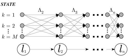
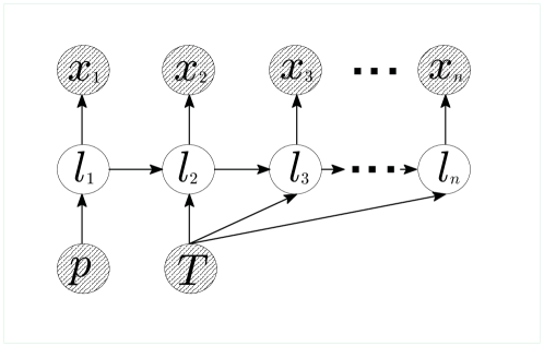
Figure 6.2.1: Trellis diagram (top) and DAG (bottom) for HMC. $\boldsymbol{\Lambda}_{i}$ are the transition metric lengths at time $i$.

6.2.1 Sequence of marginals for general label field

The purpose of this sub-section is to study the computational load when we confine the inference from the $M^{n}$-term joint $f(L_{n}|\mathbf{x}_{n})$ to just $n$ smoothing inference $f(l_{i}|\mathbf{x}_{n})=\sum_{L_{\backslash i}}f(L_{n}|\mathbf{x}_{n})$, where $L_{\backslash i}$ is the complement of $l_{i}$ in $L_{n}$, $i\in\{1,\ldots,n\}$. The general (not necessarily Markov-constrained) model $f(\mathbf{x}_{n},L_{n})$ for label field $L_{n}$ will be studied in this sub-section, while the HMC model will be studied in next sub-section.

6.2.1.1 Scalar factorization for label field

Firstly, let us investigate why direct marginalization over the joint $f(L_{n}|\mathbf{x}_{n})\propto f(\mathbf{x}_{n},L_{n})$ is intractable. By the general chain rule, any general model $f(\mathbf{x}_{n},L_{n})$ can be factorized into scalar factors, as follows:

$$f(\mathbf{x}_{n},L_{n})=\prod_{i=2}^{n}f(x_{i},l_{i}|\mathbf{x}_{i-1},L_{i-1})f(x_{1},l_{1})$$ (6.2.5)

Now, let us examine the cost of computing the sequence of posterior marginals: because there are $n$ multiplication factors in (6.2.5), the probability $f(\mathbf{x}_{n},L_{n})$ of each trajectory $L_{n}$, given $\mathbf{x}_{n}$, needs $O(n)$ of MUL operators. In order to marginalize out $L_{\backslash i}$, for each $f(l_{i}|\mathbf{x}_{n})$, we have to evaluate all probabilities of $M^{n-1}$ trajectories $L_{\backslash i}$, i.e. $M^{n-1}\times O(n)\approx O(nM^{n})$ of MULs in total. Finally, for $n$ smoothings $f(l_{i}|\mathbf{x}_{n})$, we would need $n\times O(nM^{n-1})\approx O(n^{2}M^{n})$ of MULs, which increases exponentially with $n$.

6.2.1.2 Binary partitions for label field

Apart from scalar factors, the general model (6.2.5) can also be factorized into two forward and backward sub-trajectories, $L_{i}$ and $L_{i+1:n}$, respectively:

$$f(\mathbf{x}_{n},L_{n})=f(\mathbf{x}_{i+1:n},L_{i+1:n}|\mathbf{x}_{i},L_{i})f(\mathbf{x}_{i},L_{i})$$ (6.2.6)

where $i\in\{1,\ldots,n\}$. Those two sub-trajectories, in turn, can be binarily factorized in the manner of a binary tree:

$$f(\mathbf{x}_{i},L_{i}) = f(x_{i},l_{i}|\mathbf{x}_{i-1},L_{i-1})f(\mathbf{x}_{i-1},L_{i-1})$$ (6.2.7)

$$f(\mathbf{x}_{i:n},L_{i:n}|\mathbf{x}_{i-1},L_{i-1}) = f(x_{i},l_{i}|\mathbf{x}_{i-1},L_{i-1})f(\mathbf{x}_{i+1:n},L_{i+1:n}|\mathbf{x}_{i},L_{i})$$

Note that, the cost of computing the sequence of posterior marginals via FB factorization (6.2.7) is at least the same as that cost in scalar factorization in (6.2.5), because there is no CI structure for $L_{n}$ in original $n$ factors (6.2.5). Nevertheless, when the general model (6.2.6) is specialized to the HMC model, the FB factorization (6.2.7) will lead to the tractable FB algorithm, as explained below.

6.2.2 Sequence of marginals for the HMC

By exploiting Markovianity in the HMC model, the FB algorithm, firstly proposed in [Baum et al. (1970)], computes all smoothings $f(l_{i}|\mathbf{x}_{n})$ in a recursive way, without the need to compute the $M^{n}$ values of $f(L_{n}|\mathbf{x}_{n})$ explicitly. In this sub-section, the traditional FB algorithm will be re-interpreted as a recursive update of Bayesian sufficient statistics. This fully Bayesian treatment will be helpful in understanding the underlying methodology, which we will later present in Section 6.3 on point estimation.

The recursive FB algorithm, as shown below, can divide the trajectory $L_{n}$ into sub-trajectories and reduce the complexity down from exponential form $O(n^{2}M^{n})$ in (6.2.5) down to linear form $\mathcal{O}(2nM^{2})$ of MUL. For this purpose, let us study the scalar factorization in our HMC model first.

6.2.2.1 Markovianity

Multiplying the id observation model (6.2.2) by the HMC prior (6.2.3), the joint distribution for the HMC context is:

$$f(\mathbf{x}_{n},L_{n}|\mathbf{T},p) = f(\mathbf{x}_{n}|L_{n})f(L_{n}|\mathbf{T},p)$$

$$= \prod_{i=2}^{n}f(x_{i},l_{i}|l_{i-1},\mathbf{T})f(x_{1},l_{1}|p)$$

in which we have exploited Markovianity of $L_{n}$. The augmented form for $x_{i}$ and $l_{i}$, $i\in\{1,\ldots,n\}$, is:

$$f(x_{1},l_{1}|p) = f(x_{1}|l_{1})f(l_{1}|p)$$ (6.2.9)

$$f(x_{i},l_{i}|l_{i-1},\mathbf{T}) = f(x_{i}|l_{i})f(l_{i}|l_{i-1},\mathbf{T})$$

By comparing the general model (6.2.5) with the HMC model (6.2.2.1), we can recognize the following Markov property, which will be exploited throughout the chapter:

$$f(x_{i},l_{i}|l_{i-1})=f(x_{i},l_{i}|\mathbf{x}_{i-1},L_{i-1})$$ (6.2.10)

6.2.2.2 FB recursion

Let us substitute Markov property (6.2.10) into (6.2.7) and marginalize the result in (6.2.6). In this way, we can evaluate the smoothing marginals $f(l_{i}|\mathbf{x}_{n})\propto\sum_{L_{\backslash i}}f(\mathbf{x}_{n},L_{n})$ via generalized distributive law (GDL) (Section 5.4), as follows:

$$f(l_{i}|\mathbf{x}_{n})\propto f(\mathbf{x}_{i+1:n}|l_{i})f(l_{i}|\mathbf{x}_{i})$$ (6.2.11)

in which the two marginalized sub-trajectories $f(l_{i}|\mathbf{x}_{i})\propto\sum_{L_{i-1}}f(\mathbf{x}_{i},L_{i})$ and $f(\mathbf{x}_{i+1:n}|l_{i})=\sum_{L_{i+1:n}}f(\mathbf{x}_{i+1:n},L_{i+1:n}|l_{i})$, in turn, can be computed recursively:

$$f(l_{i}|\mathbf{x}_{i}) \propto \sum_{l_{i-1}}f(x_{i},l_{i}|l_{i-1})f(l_{i-1}|\mathbf{x}_{i-1})$$ (6.2.12)

$$f(\mathbf{x}_{i:n}|l_{i-1}) = \sum_{l_{i}}f(x_{i},l_{i}|l_{i-1})f(\mathbf{x}_{i+1:n}|l_{i})$$

where $i\in\{1,\ldots,n\}$. By replacing direct marginalizations of $L_{i-1}$ and $L_{i+1:n}$ in (6.2.7) with the chain rule for marginalization (6.2.12), we have greatly reduced the total computational load of $O(M^{n-i})$ and $O(M^{i-1})$, for each time $i$, down to $O(M^{2})$ and $O(M^{2})$, respectively. Hence, the cost for all $n$ smoothings $f(l_{i}|\mathbf{x}_{n})$ is $O(2nM^{2})$.

Remark 6.2.1.

Note that, recognizing Markovianity (6.2.10) is the vital step for this scheme. Otherwise, the distributive law cannot be applied to general model (6.2.6) to yield (6.2.11). In this sense, the FB factorization (6.2.6-6.2.7) is a natural way to exploit the conditional independent (CI) structure in the HMC, thereby reducing the complexity via the generalized distributive law (GDL) (see Sections 5.4, 5.5.2.1).

6.2.2.3 FB algorithm

From (6.2.4), (6.2.9) and (6.2.12), the shaping parameters $\alpha_{i}$ for filtering marginals, $f(l_{i}|\mathbf{x}_{i})=Mu_{l_{i}}(\alpha_{i})$, as well as the un-normalized length-$M$ vector statistics $\beta_{i}\equiv\beta_{i}(\mathbf{x}_{i+1:n})$ governing the backward observations model $f(\mathbf{x}_{i+1:n}|l_{i})=l_{i}^{\prime}\beta_{i}$, $i=1,\ldots,n$, can be evaluated recursively and in parallel, as follows:

$$\alpha_{1} \propto \psi_{1}\circ p$$ (6.2.13)

$$\alpha_{i} \propto \psi_{i}\circ(\mathbf{T}\alpha_{i-1}),\ i=2,\ldots,n$$

where $\psi_{i}$ are the soft-classification vectors (6.2.1), and:

$$\beta_{n} = \boldsymbol{1}_{M\times 1}$$ (6.2.14)

$$\beta_{i} = \mathbf{T}^{\prime}(\psi_{i}\circ\beta_{i+1}),\ i=n-1,\dots,1$$

By substituting (6.2.13-6.2.14) into (6.2.11), the shaping parameters, $\gamma_{i}$, of the smoothing marginals, $f(l_{i}|\mathbf{x}_{n})=Mu_{l_{i}}(\gamma_{i})$, can be readily evaluated:

$$\gamma_{i}\propto\beta_{i}\circ\alpha_{i},\ i=\{1,\ldots,n\}$$ (6.2.15)

.

The FB algorithm, firstly proposed in [Baum et al. (1970)], consists of simultaneous forward (6.2.13) and backward (6.2.14) recursions for computing $\alpha_{i}$ and $\beta_{i}$, respectively. However, the $\beta_{i}$ evaluation (6.2.14) typically incurs a memory overflow. Stabilization is achieved via a normalization step, which was firstly proposed in [Rabiner (1989)], as shown in Algorithm 6.1.

Storage: $2n$ length-$M$ vectors $\alpha_{i}$, $\beta_{i}$ in (6.2.13-6.2.14)

Recursion: evaluate (6.2.13-6.2.14), and normalize $\beta_{i}:=\beta_{i}$ /$\sum_{k=1}^{M}\beta_{k,i}$

Termination: Evaluate $\gamma_{i}\propto\beta_{i}\circ\alpha_{i}$, $i\in\{1,\dots,n\}$.

Return $\widehat{l}_{i}=\arg\max_{l_{i}}(\gamma_{i}^{\prime}l_{i})$, $i=1,\dots,n$.

Algorithm 6.1 FB algorithm

6.3 Point estimation for HMC

In practice, it is often desired to compute point estimate $\widehat{L_{n}}=[\widehat{l_{1}},\ldots,\widehat{l_{n}}]$ for the hidden label field. For those discrete labels, the mode is a reasonable estimate. However, in general, the decision on what inference should be used leads to a trade-off between performance and computational load, as shown below.

6.3.1 HMC estimation via Maximum likelihood (ML)

If the HMC prior $f(L_{n}|\mathbf{T},p)$ is neglected, we can directly evaluate ML estimate $\widehat{L_{n}}=\arg\max_{L_{n}}f(\mathbf{x}_{n}|L_{n})=\arg\max_{L_{n}}\prod_{i=1}^{n}f(x_{i}|l_{i})$, as follows: $\widehat{l_{i}}=\arg\max_{l_{i}}\left(l_{i}^{\prime}\psi_{i}\right)$, where $i\in\{1,\ldots,n\}$. Because the maximization operator is very fast and straightforward, the computational complexity of ML estimator is very low and no memory is required.

6.3.2 HMC estimation via the MAP of marginals

The sequence of marginal MAP can be defined as $\widehat{l_{i}}=\arg\max_{l_{i}}f(l_{i}|\mathbf{x}_{n})$, $i\in\{1,\ldots,n\}$. The smoothing marginals, $f(l_{i}|\mathbf{x}_{n})$, are provided by the output of FB algorithm (6.2.15), i.e. $\widehat{l_{i}}=\arg\max_{l_{i}}(l_{i}^{\prime}\mbox{$\gamma_{i}$)}$.

Notice that the sequence of marginal MAP may be a zero-probability trajectory [Cappe et al. (2005); Fraser (2008)]. Hence, in many cases, the joint MAP of the length-$n$ trajectory, $L_{n}$, is preferred, since it is always a non-zero-probability trajectory. We address this task next.

6.3.3 HMC estimation via the MAP of trajectory

By Bayes’ rule, the MAP of trajectory is $\widehat{L}_{n}=\underset{L_{n}}{\arg\max}f(L_{n}|\mathbf{x}_{n})=\underset{L_{n}}{\arg\max}f(\mathbf{x}_{n},L_{n})$. Because maximizing $f(L_{n}|\mathbf{x}_{n})$ directly over $M^{n}$ trajectories is prohibitive, we will compute $\widehat{L}_{n}$ sequentially via $\widehat{l_{i}}\in\widehat{L_{n}}$, $i\in\{1,\ldots,n\}$. This can be achieved via two approaches: parallel memory-extraction (bi-directional VA) and recursive memory-extraction (VA). In order to understand the underlying methodology of the latter, we will present the former first.

6.3.3.1 Bi-directional VA

The computation of the MAP element $\widehat{l_{i}}\in\widehat{L_{n}}$, as defined above, will be tractable if we extract it, not from the joint inference, $f(L_{n}|\mathbf{x}_{n})$, but from $n$ profile smoothing inferences:

$$f_{p}(l_{i}|\mathbf{x}_{n})\triangleq f(l_{i}|\widehat{L}_{\backslash i},\mathbf{x}_{n})\propto\max_{L_{\backslash i}}f(\mathbf{x}_{n},L_{n})$$

where $i\in\{1,2,\ldots,n\}$. Then, we have:

$$\widehat{l_{i}}=\arg\max_{l_{i}}f_{p}(l_{i}|\mathbf{x}_{n}),\ i\in\{1,\ldots,n\}$$ (6.3.1)

In the same binary-tree approach of the FB algorithm (6.2.11), applying the Markov property (6.2.10) to the joint model (6.2.6) and maximizing the result, we have:

$$f_{p}(l_{i}|\mathbf{x}_{n})\propto f_{p}(\mathbf{x}_{i+1:n}|l_{i})f_{p}(l_{i}|\mathbf{x}_{i})$$ (6.3.2)

in which the profile filtering inferences $f_{p}(l_{i}|\mathbf{x}_{i})\equiv f(l_{i}|\widehat{L}_{i-1},\mathbf{x}_{i})\propto\max_{L_{i-1}}f(\mathbf{x}_{i},L_{i})$ and backward profile observations $f_{p}(\mathbf{x}_{i:n}|l_{i-1})\equiv f(\mathbf{x}_{i:n}|\widehat{L}_{i:n},l_{i-1})\propto\max_{L_{i:n}}f(\mathbf{x}_{i:n},L_{i:n}|l_{i-1})$, can be maximized recursively:

$$f_{p}(l_{i}|\mathbf{x}_{i}) \propto \max_{l_{i-1}}f(x_{i},l_{i}|l_{i-1})f_{p}(l_{i-1}|\mathbf{x}_{i-1})$$ (6.3.3)

$$f_{p}(\mathbf{x}_{i:n}|l_{i-1}) \propto \max_{l_{i}}f(x_{i},l_{i}|l_{i-1})f_{p}(\mathbf{x}_{i+1:n}|l_{i})$$ (6.3.4)

where $i\in\{1,\ldots,n\}$. By replacing the marginalizations (6.2.11) in the FB algorithm with maximizations, we can evaluate profile distributions in (6.3.2) in $\log$ domain, which reduces the computational load from $O(2nM^{2})$ multiplications for FB, down to $O(2nM^{2})$ additions, with the addition being much faster than multiplication in practice. This variant scheme is well known as bi-directional VA in the literature [Viterbi (1998)]. The bi-directional VA is also called soft-output variant of VA [Moon (2005)], because it produces both hard and soft information, i.e. both $\widehat{l_{i}}$ and $f_{p}(l_{i}|\mathbf{x}_{n})$, respectively.

6.3.3.2 The Viterbi Algorithm (VA)

In the second approach, which is the traditional VA, we will, once again, exploit Markovianity and further reduce computational load by establishing time-variant relations $h_{i}$: $\widehat{l_{i-1}}=h_{i}(\widehat{l_{i}})$, $i\in\{2,\ldots,n\}$, where $\widehat{l_{i}}\in\widehat{L_{n}}$, the joint MAP of trajectory, as before. Then, in the HMC, these $\widehat{l_{i}}$ can be computed recursively, without the need to evaluate the profile distributions $f_{p}(l_{i}|\mathbf{x}_{n})$, as in (6.3.1).

For motivation, let us evaluate the pair $\{\widehat{l_{i-1}},\widehat{l_{i}}\}$ via second-order of profile smoothing distributions $f_{p}(l_{i-1},l_{i}|\mathbf{x}_{n})\triangleq f(l_{i-1},l_{i}|\widehat{L}_{\backslash\{i-1,i\}},\mathbf{x}_{n})$, expanded from the first-order profiles (6.3.2), as follows:

$$f_{p}(l_{i-1},l_{i}|\mathbf{x}_{n})\propto f_{p}(\mathbf{x}_{i+1:n}|l_{i})f(x_{i},l_{i}|l_{i-1})f_{p}(l_{i-1}|\mathbf{x}_{i-1})$$ (6.3.5)

with $i\in\{2,\ldots,n\}$. Hence, the second way to find $\{\widehat{l_{i-1}},\widehat{l_{i}}\}$ is a stage wise maximization, in which we need to find one of them first, $\widehat{l_{i}}=\arg\max_{l_{i}}(\max_{l_{i-1}}f_{p}(l_{i-1},l_{i}|\mathbf{x}_{n}))$, and then substitute $l_{i}=\widehat{l_{i}}$ into (6.3.5), from which $\widehat{l_{i-1}}=h_{i}(l_{i}=\widehat{l_{i}})$, $i\in\{2,\ldots,n\}$, may be computed as follows:

$$\widehat{l_{i-1}} \triangleq\arg\max_{l_{i-1}}f_{p}(l_{i-1}|l_{i}=\widehat{l_{i}},\mathbf{x}_{n})$$

$$=\arg\max_{l_{i-1}}(f(x_{i},l_{i}=\widehat{l_{i}}|l_{i-1})f_{p}(l_{i-1}|\mathbf{x}_{i-1}))$$ (6.3.6)

$$\triangleq h_{i}(\widehat{l_{i}})$$

where (6.3.6) follows from (6.3.5) and the factor $f_{p}(\mathbf{x}_{i+1:n}|l_{i}=\widehat{l_{i}})$ was excluded in $\arg\max$ operator in (6.3.6). In this way, $h_{i}(l_{i})$ can be recognized as a conditional certainty equivalence (CE): $h_{i}(l_{i})=\widehat{l_{i-1}}(l_{i})\triangleq\arg\max_{l_{i-1}}f_{p}(l_{i-1}|l_{i},\mathbf{x}_{n})$. Moreover, comparing (6.3.6) with (6.3.3), we can see that $h_{i}(l_{i})$ are consequences of the forward step and, hence, its values can be stored in the memory in an online manner. Given $\widehat{l_{n}}$ at the end of the forward step, i.e. via (6.3.1), we can directly trace back all other labels $\widehat{l_{n-1}},\ldots,\widehat{l_{1}}$ via the stored values $\widehat{l_{i-1}}=h_{i}(\widehat{l_{i}})$, $i\in\{2,\ldots,n\}$, without the need to evaluate the backward step (6.3.4) and profile smoothing distributions (6.3.1-6.3.2). Hence, VA halves the computational load of bi-directional VA by requiring computation of the forward step (6.3.3) only.

Now, we can formalize VA via two steps, as detailed next.

Viterbi Forward step

By substituting (6.2.4) into (6.2.9), we can express $f(x_{i},l_{i}|l_{i-1})$ in (6.3.3) in exponential form, as follows:

$$f(x_{1},l_{1}|p) =\exp(-l_{1}^{\prime}\boldsymbol{\lambda}_{1})$$ (6.3.7)

$$f(x_{i},l_{i}|l_{i-1},\mathbf{T}) =\mbox{$\exp$}(-l_{i}^{\prime}\boldsymbol{\Lambda}_{i}l_{i-1}),\ i=2,\dots,n$$

in which the sufficient statistics $\boldsymbol{\lambda}_{i}$, collected into a sequence of $n$ length-$M$ vectors, and the information measures $\boldsymbol{\Lambda}_{i}\equiv\boldsymbol{\Lambda}_{i}(x_{i})$, being a sequence of $n-1$ $M\times M$ matrices, can be defined as follows:

$$\boldsymbol{\lambda}_{1} = -(\log(\psi_{i})+\log p)$$ (6.3.8)

$$\boldsymbol{\Lambda}_{i} = -(\log(\psi_{i}\mathbf{1}_{M\times 1}^{\prime})+\log\mathbf{T}),\ i=2,\dots,n$$ (6.3.9)

where $\psi_{i}$ are the soft-classification vectors (6.2.1).

Finally, substituting (6.3.7) back into (6.3.3), the shaping parameters $\overline{\alpha}_{i}$ of the profile filtering distributions $f_{p}(l_{i}|\mathbf{x}_{i})=Mu_{l_{i}}(\overline{\alpha}_{i})$ in (6.3.3), $i\in\{1,\ldots,n\}$, can be evaluated in log-domain as follows:

$$\overline{\alpha}_{i}\propto\exp(-\boldsymbol{\lambda}_{i})$$ (6.3.10)

$$\boldsymbol{\lambda}_{j,i} = \min_{k}(\boldsymbol{\Lambda}_{i}(j,k)+\boldsymbol{\lambda}_{k,i-1})$$ (6.3.11)

$$\kappa_{j,i} = \arg\min_{k}(\boldsymbol{\Lambda}_{i}(j,k)+\boldsymbol{\lambda}_{k,i-1})$$ (6.3.12)

where $\boldsymbol{\lambda}_{j,i}$ and $\kappa_{j,i}$, $j\in\{1,\ldots,M\}$, denote $j$th element of vectors $\boldsymbol{\lambda}_{i}$ and $\kappa_{i}$, respectively, and $\boldsymbol{\Lambda}_{i}(j,k)$ denotes element at $j$th row and $k$th column of matrix $\boldsymbol{\Lambda}_{i}$, $1\leq j,k\leq M$. Note that the conditional CEs $\widehat{l_{i-1}}(l_{i})$ in (6.3.6) can be found feasibly via (6.3.12): $h_{i}(l_{i})=\widehat{l_{i-1}}(l_{i})=\epsilon(l_{i}^{\prime}\kappa_{i})$, $i\in\{2,\ldots,n\}$, where $\epsilon(j)$ in general denotes the $j$th elementary vector in $\mathbb{R}^{M}$.

In the literature, $\boldsymbol{\lambda}_{i}$ and $\boldsymbol{\Lambda}_{i}$ are not given this novel Bayesian perspective. Indeed, the term “metric length” is often assigned to the elements $\boldsymbol{\Lambda}_{i}(j,k)$ [Forney (1973)], owing to their positive value and representation as an edge in trellis diagram (Fig. 6.2.1).

Moreover, the forward recursions of profile filterings $f_{p}(l_{i}|\mathbf{x}_{i})$ in (6.3.3) are often considered as maintaining $M$ “survival” maximal trajectories, reduced from the original $M^{i}$ trajectories in $f(L_{i}|\mathbf{x}_{i})$. The reason for this language is the fact that one of the $M$ length-$i$ trajectories in $f_{p}(l_{i}|\mathbf{x}_{i})$ is the prefix of the global MAP trajectory $\widehat{L}_{n}$. Hence, each element $\boldsymbol{\lambda}_{j,i}$ in (6.3.11) is often called the “weighted length” of the $j$th survival trajectory at time $i$, $j\in\{1,\ldots,M\}$ [Forney (1973)].

Viterbi back-tracking step

From (6.3.6), the joint MAP trajectory, $\widehat{L}_{n}$, can be evaluated via a fast backward recursion. The last label estimate is found first, i.e. we have $\widehat{l_{n}}=\underset{l_{n}}{\arg\max}f_{p}(l_{n}|\mathbf{x}_{n})=\boldsymbol{\epsilon}(\widehat{k}_{n})$, where:

$$\widehat{k}_{n}=\underset{j}{\arg\min}(\boldsymbol{\lambda}_{j,n})$$ (6.3.13)

Then, the previous labels $\widehat{l_{i-1}}=\widehat{l_{i-1}}(l_{i}=\widehat{l_{i}})=\boldsymbol{\epsilon}(\widehat{k}_{i-1})$, $i=2,\dots,n,$ leading to $\widehat{l_{n}}$, can be recursively traced back using the $\kappa_{i}$ vectors of Viterbi forward step (6.3.12), as follows:

$$\widehat{k}_{i-1}=\kappa_{j=\widehat{k}_{i},i}$$ (6.3.14)

Remark 6.3.1.

Notice that, Markovianity is the vital condition, exploited by the VA in computational reduction. Without it, the $\max$ operators cannot be distributed recursively in (6.3.2). Computation, both the recursive addition in (6.2.12) and maximization in (6.3.2) are special cases of the generalized distributive law (GDL) (see Sections 5.4, 5.5.2.2).

Viterbi algorithm

The VA, firstly presented in [Viterbi (1967)] for channel decoding context, was formalized via trellis diagram for the HMC in [Forney (1973)] (Fig. 6.2.1). Note that the MAP of trajectory may change entirely based on the last observation $x_{n}$, owing to (6.3.13). The VA (Algorithm 6.2) is, therefore, an offline (batch-based) algorithm.

Storage: Length-$M$ vectors $\kappa_{i}$, $i\in\{1,\ldots,n\}$, as in (6.3.12)

Initialization: evaluate (6.3.8)

Recursion: For $i\in\{1,\ldots,n\}$: evaluate (6.3.8-6.3.9) and (6.3.11-6.3.12)

Termination: evaluate (6.3.13- 6.3.14)

Return $\widehat{l}_{i}=\boldsymbol{\epsilon}(\widehat{k}_{i})$, $i=1,\dots,n$.

Algorithm 6.2 Viterbi Algorithm (with similar convention to [Forney (1973)])

6.4 Re-interpretation of FB and VA via CI factorization

In the Bayesian viewpoint, the Markov property (6.2.10) not only reduces the computational load for inference on the joint model (6.2.6), but fundamentally, also yields a CI factorization (6.2.2.1) for posterior distribution of label field. In this section, we will re-interpret the outputs of FB and VA, and show that they are merely a consequence of CI structure, i.e. FB returns the shaping parameters of HMC re-factorization, while VA returns the shaping parameters of a degenerated HMC.

6.4.1 Inhomogeneous HMC

In the literature, it has been shown that the posterior distribution of hidden label field, given id observations (6.2.2) and prior homogeneous HMC (6.2.3), is an inhomogeneous HMC [Cappe et al. (2005)]. In this sense, HMC prior (6.2.3) is a conjugate prior of id observation model (6.2.2), in the sense defined in Section 4.4.2.4. We will clarify this result via the following proposition:

Proposition 6.4.1.

The posterior distribution of the homogeneous HMC (6.2.3), given conditionally id observation (6.2.2), is an inhomogeneous HMC:

$$f(L_{n}|\mathbf{x}_{n}) = f(L_{i+1:n}|l_{i},\mathbf{x}_{n})f(l_{i}|\mathbf{x}_{n})f(L_{i-1}|L_{i:n},\mathbf{x}_{n})$$ (6.4.1)

in which $i\in\{1,\ldots,n\}$ and:

$$f(L_{i-1}|L_{i:n},\mathbf{x}_{n})=f(L_{i-1}|l_{i},\mathbf{x}_{i-1}) = \prod_{j=1}^{i-1}f(l_{j}|l_{j+1},\mathbf{x}_{j})$$ (6.4.2)

$$f(L_{i+1:n}|L_{i},\mathbf{x}_{n})=f(L_{i+1:n}|l_{i},\mathbf{x}_{i+1:n}) = \prod_{j=i+1}^{n}f(l_{j}|l_{j-1},\mathbf{x}_{j:n})$$

Proof.

Note that (6.4.1) simply follows the probability chain rule for any general distribution $f(L_{n}|\mathbf{x}_{n})$. For the proof of (6.4.2), substituting Markov property (6.2.10) into the joint inference (6.2.6), we have:

$$f(L_{i-1}|L_{i:n},\mathbf{x}_{n}) = \frac{f(\mathbf{x}_{n},L_{n})}{\sum_{L_{i-1}}f(\mathbf{x}_{n},L_{n})}=\frac{f(\mathbf{x}_{i-1},L_{i})}{\sum_{L_{i-1}}f(\mathbf{x}_{i-1},L_{i})}$$

$$= f(L_{i-1}|l_{i},\mathbf{x}_{i-1}),\ \forall i\in\{1,\ldots,n\}$$

$$f(L_{i:n}|L_{i-1},\mathbf{x}_{n}) = \frac{f(\mathbf{x}_{n},L_{n})}{\sum_{L_{i:n}}f(\mathbf{x}_{n},L_{n})}=\frac{f(\mathbf{x}_{i:n},L_{i:n}|l_{i-1})}{\sum_{L_{i:n}}f(\mathbf{x}_{i:n},L_{i:n}|l_{i-1})}$$

$$= f(L_{i:n}|l_{i-1},\mathbf{x}_{i:n}),\ \forall i\in\{1,\ldots,n\}$$

Because the above equations are valid for all $i\in\{1,\ldots,n\}$, we can derive the right hand side of (6.4.2) by induction. ∎

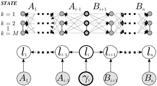
Figure 6.4.1: Posterior distribution of HMC in Fig. 6.2.1, via FB algorithm: trellis diagram (top) and DAG (bottom). Symbols are explained in the text.

Note that, the FB algorithm (Algorithm 6.1) is actually implied by the CI factorization in (6.4.1), as shown in Propositions 5.5.1,5.5.2. Then, the backward transitions probabilities:

$$f(l_{i-1}|l_{i},\mathbf{x}_{i})=\frac{f(x_{i},l_{i},l_{i-1}|\mathbf{x}_{i-1})}{\sum_{l_{i}}f(x_{i},l_{i},l_{i-1}|\mathbf{x}_{i-1})}$$

and forward transitions probabilities:

$$f(l_{i}|l_{i-1},\mathbf{x}_{i:n})=\frac{f(\mathbf{x}_{i:n},l_{i}|l_{i-1})}{\sum_{l_{i}}f(\mathbf{x}_{i:n},l_{i}|l_{i-1})}$$

in (6.4.2) can be computed via second-order filtering marginals:

$$f(x_{i},l_{i},l_{i-1}|\mathbf{x}_{i-1})=f(x_{i},l_{i}|l_{i-1})f(l_{i-1}|\mathbf{x}_{i-1})$$

and backward observation model:

$$f(\mathbf{x}_{i:n},l_{i:n}|l_{i-1})=f(x_{i},l_{i}|l_{i-1})f(\mathbf{x}_{i+1:n}|l_{i})$$

extracted from forward and backward recursions in (6.2.12), respectively. The following corollary will clarify this fact.

Corollary 6.4.2.

The posterior distributions in (6.4.2) can be evaluated via FB algorithm (Algorithm 6.1), as follows:

$$f(l_{i}|\mathbf{x}_{n}) = Mu_{l_{i}}(\gamma_{i}),\ i\in\{1,\ldots,n\}$$ (6.4.3)

$$f(l_{i}|l_{i+1},\mathbf{x}_{i}) = Mu_{l_{i}}(A_{i}^{\prime}l_{i+1}),\ i\in\{2,\ldots,n\}$$

$$f(l_{i+1}|l_{i},\mathbf{x}_{i+1:n}) = Mu_{l_{i+1}}(B_{i}l_{i}),\ i\in\{1,\ldots,n-1\}$$

where $A_{i}(k,:)\propto\mathbf{T}(k,:)\circ\alpha_{i}^{\prime}$ and $B_{i}(:,k)\propto\beta_{i+1}\circ\boldsymbol{\Lambda}_{i}(:,k)$ are right- and left-stochastic matrices of sufficient statistics, with $(k,:)$ and $(:,k)$ denoting $k$th row and $k$th column of a matrix, respectively, as illustrated in Fig 6.4.1.

Proof.

By the chain rule, we have:

$$f(l_{i}|l_{i+1},\mathbf{x}_{i}) = \frac{f(l_{i+1}|l_{i})f(l_{i}|\mathbf{x}_{i})}{\sum_{l_{i}}f(l_{i+1}|l_{i})f(l_{i}|\mathbf{x}_{i})}$$ (6.4.4)

$$f(l_{i+1}|l_{i},\mathbf{x}_{i+1:n}) = \frac{f(\mathbf{x}_{i+1:n}|l_{i+1})f(l_{i+1}|l_{i})}{\sum_{l_{i+1}}f(\mathbf{x}_{i+1:n}|l_{i+1})f(l_{i+1}|l_{i})}$$ (6.4.5)

Notice that all of the terms in right hand side (6.4.3-6.4.5) have been derived in (6.2.13-6.2.15). ∎

6.4.2 Profile-approximated HMC

In order to find the joint MAP of trajectory, $\widehat{L}_{n}$, the bi-directional VA computed a sequence of profile distributions $f_{p}(l_{i}|\mathbf{x}_{n})$ via bi-directional maximization (6.3.2-6.3.4) on joint model (6.2.2.1). Since joint model (6.2.2.1) can be re-factorized into CI structure (6.4.1), then, applying the same bi-directional maximization to (6.4.1), we can define $n$ approximated HMCs, corresponding to each choice of $i\in\{1,\ldots,n\}$ in (6.4.1), as follows:

$$\overline{f}_{i}(L_{n}|\mathbf{x}_{n})=\left(\prod_{j=i+1}^{n}f_{p}(l_{j}|l_{j-1},\mathbf{x}_{j:n})\right)f_{p}(l_{i}|\mathbf{x}_{n})\left(\prod_{j=1}^{i-1}f_{p}(l_{j}|l_{j+1},\mathbf{x}_{j})\right)$$ (6.4.6)

where $i\in\{1,\ldots,n\}$, and:

$$f(l_{i}|\mathbf{x}_{n}) \propto \max_{L_{\backslash i}}f(L_{i}|\mathbf{x}_{i})$$ (6.4.7)

$$f_{p}(l_{j}|l_{j+1},\mathbf{x}_{j}) \propto \max_{L_{j-1}}f(L_{j}|l_{j+1},\mathbf{x}_{j})$$

$$f_{p}(l_{j}|l_{j-1},\mathbf{x}_{j:n}) \propto \max_{L_{j+1:n}}f(L_{j:n}|l_{j-1},\mathbf{x}_{j:n})$$

In common with the FB algorithm, the backward and forward transition probabilities in (6.4.7) are, respectively:

$$f_{p}(l_{j}|l_{j+1},\mathbf{x}_{j}) = \frac{f_{p}(\mathbf{x}_{j},l_{j},l_{j+1})}{\sum_{l_{j}}f_{p}(\mathbf{x}_{j},l_{j},l_{j+1})}$$

$$f_{p}(l_{j}|l_{j-1},\mathbf{x}_{j:n}) = \frac{f(\mathbf{x}_{j:n},l_{j},l_{j-1})}{\sum_{l_{j}}f(\mathbf{x}_{j:n},l_{j},l_{j-1})}$$

which can be computed via second-order profile filterings and profile backward observation:

$$f_{p}(\mathbf{x}_{i},l_{i},l_{i+1}) = f(x_{i},l_{i}|l_{i-1})f_{p}(l_{i-1}|\mathbf{x}_{i-1})$$

$$f_{p}(\mathbf{x}_{i:n},l_{i},l_{i-1}) = f(x_{i},l_{i}|l_{i-1})f_{p}(\mathbf{x}_{i+1:n}|l_{i})$$

These, in turn, can be extracted from forward and backward recursions in (6.3.3-6.3.4), respectively.

Note that, because of normalization constants involved in (6.4.7), applying the bi-directional VA algorithm (6.3.2) to (6.4.6) will not recover the three $\max$ terms on the right hand side of (6.4.7). Hence, the joint MAP of $\overline{f}_{i}(L_{n}|\mathbf{x}_{n})$ is different from the original joint MAP of $f(L_{n}|\mathbf{x}_{n})$ in general. However, the sequence of modes of the $n$ marginals $f_{p}(l_{i}|\mathbf{x}_{n})$ in the $n$ approximations $\overline{f}_{i}(L_{n}|\mathbf{x}_{n})$ is actually the same as the original joint MAP $\widehat{L}_{n}$ of $f(L_{n}|\mathbf{x}_{n})$.

If we neglect the normalization in (6.4.7), we can find the joint MAP more quickly via VA, as explained below.

6.4.3 CE-based approximated HMC

VA avoids the normalizations (6.4.7) in bi-directional VA by keeping only their CE values in memory. This scheme yields another $n$ CE-based approximated HMCs, as follows:

$$\widehat{f}_{i}(L_{n}|\mathbf{x}_{n})=\left(\prod_{j=i+1}^{n}f_{\delta}(l_{j}|l_{j-1},\mathbf{x}_{j:n})\right)f_{p}(l_{i}|\mathbf{x}_{n})\left(\prod_{j=1}^{i-1}f_{\delta}(l_{j}|l_{j+1},\mathbf{x}_{j})\right)$$ (6.4.8)

for $i\in\{1,\ldots,n\}$ and:

$$f_{p}(l_{i}|\mathbf{x}_{n}) = Mu_{l_{i}}(\widehat{\gamma_{i}}),\ i\in\{1,\ldots,n\}$$ (6.4.9)

$$f_{\delta}(l_{j}|l_{j+1},\mathbf{x}_{j}) = \delta[l_{j}-\widehat{l}_{j}(l_{j+1})]=Mu_{l_{j}}(\widehat{A}_{j}^{\prime}l_{j})$$ (6.4.10)

$$f_{\delta}(l_{j}|l_{j-1},\mathbf{x}_{j:n}) = \delta[l_{j}-\widehat{l}_{j}(l_{j-1})]=Mu_{l_{j}}(\widehat{B}_{j}^{\prime}l_{j})$$

in which $\widehat{A}_{j}=[\widehat{l_{j}}(l_{j+1}=\boldsymbol{\epsilon}(1))^{\prime},\ldots,\widehat{l_{j}}(l_{j+1}=\boldsymbol{\epsilon}(M))^{\prime}]^{\prime}$ and $\widehat{B}_{j}=[\widehat{l_{j}}(l_{j-1}=\boldsymbol{\epsilon}(1)),\ldots,$ $\widehat{l_{j}}(l_{j-1}=\boldsymbol{\epsilon}(M))]$ are sparse left-stochastic matrices, with only one element at each column, as illustrated in Fig. 6.4.2. The conditional CEs in (6.4.9) are defined as follows:

$$\widehat{l}_{j}(l_{j+1}) =\arg\max_{l_{j}}f_{p}(l_{j}|l_{j+1},\mathbf{x}_{j})=\arg\max_{l_{j}}f_{p}(l_{j},l_{j+1}|\mathbf{x}_{n})$$

$$\widehat{l}_{j}(l_{j-1}) =\arg\max_{l_{j}}f_{p}(l_{j}|l_{j-1},\mathbf{x}_{j:n})=\arg\max_{l_{j}}f_{p}(l_{j},l_{j-1}|\mathbf{x}_{n})$$ (6.4.11)

in which the right hand side of (6.4.11) is implied by CI structure in (6.4.1).

As explained in Section 6.3.3.2, substituting $\widehat{l}_{j+1}$and $\widehat{l}_{j-1}$ of original joint MAP of $f(L_{n}|\mathbf{x}_{n})$ into (6.4.11), we can also extract $\widehat{l}_{j}(l_{j+1})$ and $\widehat{l}_{j}(l_{j-1})$ belonging to that joint MAP. Hence, given $\widehat{l}_{i}=\arg\max_{l_{i}}f_{p}(l_{i}|\mathbf{x}_{n})$ in $\widehat{f}_{i}(L_{n}|\mathbf{x}_{n})$ for any $i\in\{1,\ldots,n\}$, we can trace back the original MAP from stored conditional CEs in (6.4.11). Although this back-tracking scheme works for any $i\in\{1,\ldots,n\}$, in practice the traditional VA always assigns $i=n$ in $\widehat{f}_{i}(L_{n}|\mathbf{x}_{n})$ and maintains profile filtering distributions $f_{p}(l_{n}|\mathbf{x}_{n})$, in order to achieve an online forward scheme for new data at time $n+1$, as illustrated in Fig. 6.4.3.

It can be proved feasibly that the joint MAP of $\widehat{f}_{i}(L_{n}|\mathbf{x}_{n})$, for any $i\in\{1,\ldots,n\}$, are the same as joint MAP $f(L_{n}|\mathbf{x}_{n})$, since they have the same conditional CEs and the same elements $\widehat{l}_{i}$ of joint MAP. Also, because $\widehat{f}(L_{n}|\mathbf{x}_{n})$ only has $M$ non-zero-probability trajectories, finding the original joint MAP via $\widehat{f}(L_{n}|\mathbf{x}_{n})$ is easier than via the exact $f(L_{n}|\mathbf{x}_{n})$.

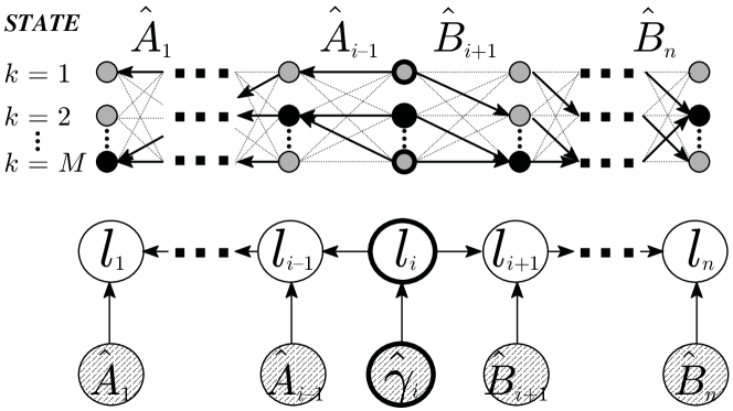
Figure 6.4.2: Bi-directional Viterbi algorithm (VA) for HMC posterior in Fig. 6.4.1: trellis diagram (top) and DAG (bottom). Dotted lines denote zero-probability transitions. Note that, black circles denote joint MAP of trajectory of $f(L_{n}|\mathbf{x}_{n})$ in (6.4.1), but a sequence of modes of $n$ marginals $f_{p}(l_{i}|\mathbf{x}_{n})$ for $\overline{f}_{i}(L_{n}|\mathbf{x}_{n})$ in (6.4.6), $i\in\{1,\ldots,n\}$.

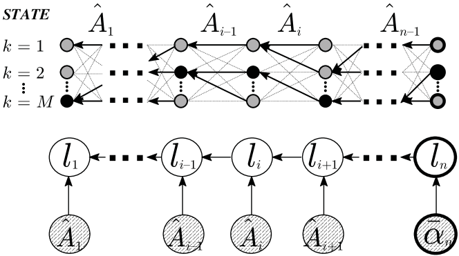
Figure 6.4.3: Viterbi algorithm (VA) for HMC posterior in Fig. 6.4.1: trellis diagram (top) and DAG (bottom), with the same convention as Fig 6.4.2. Note that, black circles denote the same joint MAP trajectory of both $f(L_{n}|\mathbf{x}_{n})$ in (6.4.1) and $\widehat{f}_{i}(L_{n}|\mathbf{x}_{n})$ in (6.4.8), for any $i\in\{1,\ldots,n\}$. These black circles and $\bar{\alpha}_{n}$ in this figure are exactly the same as the black circles and $\widehat{\gamma_{n}}$ in Fig 6.4.2, respectively, when $i=n$.

6.5 Variational Bayes (VB) approximation for CI structure

In the previous section, we have shown that VA involves a CE-based approximation of the smoothing marginals $f(l_{i}|\mathbf{x}_{n})$ in the FB algorithm. The VA reduces complexity significantly via two sequential steps:

• The first step is to constrain the inference problem, replacing the smoothing marginals, $f(l_{i}|\mathbf{x}_{n})$, with profile smoothing distributions, $f_{p}(l_{i}|\mathbf{x}_{n})$.

• The second step is further to constrain these profile smoothing distributions to point inferences and directly compute $\widehat{l_{i}}$ of the joint MAP within this CE-based distribution.

In a similar manner, we seek novel variants of VA via two sequential steps:

• The first step is to derive a distributional approximation of $f(L_{n}|\mathbf{x}_{n})$ from the class of independent distributions $\prod_{i=1}^{n}\widetilde{f}(l_{i}|\mathbf{x}_{n})$ via VB (Section 4.5.2).

• The second step is further to impose a CE-based constraint upon the VB marginals, via FCVB (Section 4.5.2.4), in order to reduce complexity significantly.

For this purpose, we will apply the VB and FCVB methodology to a general multivariate posterior distribution in this section, and then to the HMC in next section.

6.5.1 VB approximation via Kolmogorov-Smirnov (KS) distance

Let us consider a sequence of $n$ variables $\theta\triangleq\{\theta_{1},\ldots,\theta_{n}\}$, provided that there is an arbitrary choice in partition of $\theta$ into (non-empty) sub-vectors $\theta_{i}$. Then, given a joint posterior distribution $f(\theta|\mathbf{x})$, the VB method is to seek an approximated distribution, $\tilde{f}(\theta|\mathbf{x})$, in independent distribution class $\mathbb{F}_{c}$, $\breve{f}(\theta|\mathbf{x})=\prod_{i=1}^{n}\breve{f}(\theta_{i}|\mathbf{x})$, such that the Kullback-Leibler divergence:

$$KLD_{\widetilde{f}||f}\triangleq KLD(\tilde{f}(\theta|\mathbf{x})||f(\theta|\mathbf{x}))=E_{\tilde{f}(\theta|\mathbf{x})}\log\frac{\tilde{f}(\theta|\mathbf{x})}{f(\theta|\mathbf{x})}$$

is minimized, as explained in Section 4.5.2.

6.5.1.1 Iterative VB (IVB) algorithm

Given an arbitrary initial distribution $\widetilde{f}^{[0]}(\theta|\mathbf{x})=\prod_{i=1}^{n}\widetilde{f}^{[0]}(\theta_{i}|\mathbf{x})$, the aim of the IVB algorithm is to update the VB-marginals $\widetilde{f}^{[\nu]}(\theta_{i}|\mathbf{x})$ iteratively, $\nu=1,2,\ldots$, and cyclically with $\theta_{i}$, until a local minimum of $KLD_{\widetilde{f}||f}$ is reached. This is achieved as follows (Theorem 4.5.1):

$$\widetilde{f}^{[\nu]}(\theta_{i}|\mathbf{x}) \propto \exp\left(E_{\widetilde{f}^{[\nu]}(\theta_{\backslash i}|\mathbf{x})}\log f(\theta|\mathbf{x})\right),\ i\in\{1,\ldots,n\}$$ (6.5.1)

where we recall that $\theta_{\backslash i}$ denotes the complement of $\theta_{i}$ in $\theta$, and:

$$\widetilde{f}^{[\nu]}(\theta_{\backslash i}|\mathbf{x})=\prod_{j=i+1:n}\widetilde{f}^{[\nu-1]}(\theta_{j}|\mathbf{x})\prod_{j=1:i-1}.\widetilde{f}^{[\nu]}(\theta_{j}|\mathbf{x})$$

Note that, in practice, because the normalized form $f(\theta|\mathbf{x})$ is often unavailable (intractable), we can replace $f(\theta|\mathbf{x})$ with its unnormalized variant $f(\mathbf{x},\theta)$ in (6.5.1).

Also, in the IVB algorithm, we can freely permute the sequence $\{\theta_{\pi(1)},\ldots,\theta_{\pi(n)}\}$ for the update of VB-marginals (6.5.1) in any IVB cycle, where $\pi$ is a fixed permutation of the index set $\{1,\ldots,n\}$. Since we have not specified any particular order for the index set $\{1,\ldots,n\}$, let us denote, for convenience, that $\pi(i)=i$, $\forall i\in\{1,\ldots,n\}$.

6.5.1.2 Stopping rule for IVB algorithm

Because $KLD_{\widetilde{f}||f}$ in IVB algorithm is guaranteed to be non-increasing with $\nu$ in the IVB algorithm (6.5.1), and to converge to a local minimum [Smidl and Quinn (2006)], we can propose a stopping rule by choosing a small threshold $\xi_{c}$, such that $\nu_{c}\triangleq\min_{\nu}\left(KLD_{\widetilde{f}||f}^{[\nu]}\leq\xi_{c}\right)$, as in the definition of the converged cycle number, $\nu_{c}$. However, the IVB algorithm does not evaluate $KLD_{\widetilde{f}||f}^{[\nu]}$ itself and that evaluation is typically prohibitive.

Therefore, instead of using the joint $KLD_{\widetilde{f}||f}$, let us consider individual convergence of each VB-marginal via Kolmogorov-Smirnov (KS) distance [Rachev (1991)]:

$$KS_{i}^{[\nu]} \triangleq \max_{\theta_{i}}\left|\widetilde{F}^{[\nu]}(\theta_{i}|\mathbf{x})-\widetilde{F}^{[\nu-1]}(\theta_{i}|\mathbf{x})\right|$$ (6.5.2)

where $\widetilde{F}(\theta_{i}|\mathbf{x})$ denotes the cumulative distribution function (c.d.f) of $\widetilde{f}(\theta_{i}|\mathbf{x})$, $i\in\{1,\ldots,n\}$. Because verifying $KS_{i}^{[\nu]}$ requires only maximization and addition operations, this informal scheme for verifying convergence of the IVB algorithm is much faster than formal evaluation of $KLD_{\widetilde{f}||f}^{[\nu]}$ itself. Note that, IVB continues to iterate in order to decrease $KLD_{\widetilde{f}||f}$ and the KS is only proposed for the stopping rule.

Indeed, this stopping rule $KS_{i}$ for each VB-marginal is stricter than that of $KLD_{\widetilde{f}||f}$ and may lead to higher value of $\nu_{c}$. This strictness can be compensated by choosing a greater $\xi_{c}$. In this thesis, the IVB algorithm is considered to be converged at cycle $\nu_{c}$ if the following condition is satisfied:

$$KS_{i}^{[\nu_{c}]}\leq\xi=0.01,\ \forall i\in\{1,\ldots,n\}$$ (6.5.3)

In simulations, presented in Chapter 8, no gain in performance was achieved with threshold $\xi$ lower than $0.01$. Apart from the cost reduction, this KS-based stopping rule will also lead to a novel speed-up scheme for the IVB algorithm, as explained in Section 6.5.2.

For later use, let us indicate the status of $KS_{i}^{[\nu]}$, $i\in\{1,\ldots,n\}$, via a sequence of $n$ Boolean indicators $\varrho_{i}^{[\nu]}$, $i\in\{1,\ldots,n\}$, as follows:

$$\begin{cases}\varrho_{i}^{[\nu]}=0,&\mbox{if}\ KS_{i}^{[\nu]}\leq\xi\\ \varrho_{i}^{[\nu]}=1,&\mbox{if}\ KS_{i}^{[\nu]}>\xi\end{cases}\hskip 10.00002pti\in\{1,\ldots,n\},\ \nu=1,2,\ldots$$ (6.5.4)

Then, the KS-based condition (6.5.3) is equivalent to the following condition:

$$\sum_{i=1}^{n}\varrho_{i}^{[\nu_{c}]}=0,\ \mbox{or\ equivalently},\ \varrho_{i}^{[\nu_{c}]}=0,\forall i\in\{1,\ldots,n\}$$ (6.5.5)

The IVB algorithm in this case is presented in Algorithm 6.3.

Iteration:

For $\nu=1,2,\ldots$, do {

For $i=1,\ldots n$, do {

evaluate either (6.5.1) or (6.5.7)

if $KS_{i}^{[\nu]}\leq\xi$, { set $\varrho_{i}=0$ }

else: {set $\varrho_{i}=1$}}}}

Termination: stop if $\varrho_{i}=0$, $\forall i\in\{1,\ldots,n\}$

Algorithm 6.3 IVB algorithm using KS-distance stopping rule

6.5.2 Accelerated IVB approximation

In general, any joint distribution $f(\theta|\mathbf{x})$ can be binarily factorized in respect of each choice of $\theta_{i}$, $i\in\{1,\ldots,n\}$, thereby exploiting any CI structure that may be present in the joint model:

$$f(\theta|\mathbf{x})=f(\theta_{i}|\theta_{\eta_{i}},\mathbf{x})f(\theta_{\backslash i}|\mathbf{x}),\ i\in\{1,\ldots,n\}$$ (6.5.6)

where the neighbour set is $\theta_{\eta_{i}}\subseteq\theta_{\backslash i}$. Then, the key step in accelerating the IVB algorithm is to exploit the CI structure of the original distribution $f(\theta|\mathbf{x})$, as explained next.

6.5.2.1 IVB algorithm for CI structure

Owing to the CI structure (6.5.6), the IVB algorithm (6.5.1) only involves the neighbour set $\theta_{\eta_{i}}$, instead of the whole set $\theta_{\backslash i}$, as follows:

$$\widetilde{f}^{[\nu]}(\theta_{i}|\mathbf{x})\propto\exp\left(E_{\widetilde{f}^{[\nu]}(\theta_{\eta_{i}}|\mathbf{x})}\log f(\theta_{i},\theta_{\eta_{i}}|\mathbf{x})\right),\ i\in\{1,\ldots,n\}$$ (6.5.7)

where:

$$\widetilde{f}^{[\nu]}(\theta_{\eta_{i}}|\mathbf{x})=\prod_{j\in\eta_{i}^{BW}}.\widetilde{f}^{[\nu-1]}(\theta_{j}|\mathbf{x})\prod_{j\in\eta_{i}^{FW}}\widetilde{f}^{[\nu]}(\theta_{j}|\mathbf{x})$$ (6.5.8)

with $\eta_{i}^{FW}=\eta_{i}\cup\{1:i-1\}$, $\eta_{i}^{BW}=\eta_{i}\cup\{i+1:n\}$ denoting forward and backward neighbour index sets, respectively, and $\eta_{i}=\{\eta_{i}^{FW},\eta_{i}^{BW}\}$.

6.5.2.2 Accelerated IVB algorithm

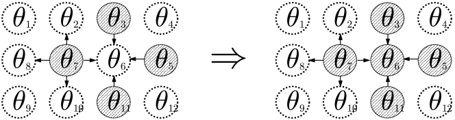
Figure 6.5.1: Many-to-one scheme. Left: VB-marginals $\widetilde{f}(\theta_{3})$, $\widetilde{f}(\theta_{5})$, $\widetilde{f}(\theta_{7})$ and $\widetilde{f}(\theta_{11})$ in current IVB cycle $\nu$ are converged (shaded nodes, i.e. $\tau^{[\nu]}=0$). Therefore, Right: $\widetilde{f}(\theta_{6})$ is set as converged ($\tau_{6}^{[\nu+1]}=0$) in next IVB cycle. White nodes denote unknown converged state of VB-marginals (unknown $\tau_{i}$).

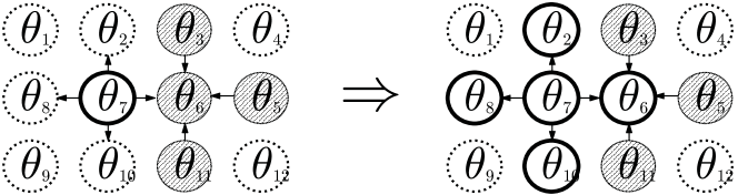
Figure 6.5.2: One-to-many scheme. Left: $\widetilde{f}(\theta_{7})$ is not converged in current IVB cycle $\nu$ (thick, black circle node $\tau_{7}^{[\nu]}=1$). Therefore, Right: $\widetilde{f}(\theta_{2})$, $\widetilde{f}(\theta_{6})$, $\widetilde{f}(\theta_{8})$ and $\widetilde{f}(\theta_{10})$ are set as not converged (i.e. $\tau^{[\nu+1]}=1)$ in the next IVB cycle. Shaded nodes denote converged VB-marginals ($\tau_{i}=0)$. Dotted circles denote unknown converged state (unknown $\tau_{i}$).

In IVB (6.5.7), we have to update all $n$ VB-marginals at any cycle $\nu$, since the KS-based conditions (6.5.4) needs to be checked all the time. Therefore, if we can quickly identify the converged VB-marginals at current IVB cycle and exclude them from next IVB cycle, the computational load will be reduced.

Hence, the central idea of the accelerated scheme is the concept of individual convergence. Nevertheless, although the convergence of $KLD_{\widetilde{f}||f}$ can be proved to be monotone [Smidl and Quinn (2006)], the individual convergence of $KS_{i}^{[\nu]}$ for each VB-marginal is not monotone in general and might vary around the threshold $\xi$. For resolving this problem, let us formulate two remarks about the CI structure (6.5.7):

• The first remark, called “many-to-one”, is that the VB-marginal, $\widetilde{f}^{[\nu]}(\theta_{i}|\mathbf{x})$, is regarded as converged and can be ignored at cycle $\nu$, if all of its neighbour VB-marginals $\widetilde{f}^{[\nu-1]}(\theta_{j}|\mathbf{x})$ in (6.5.8) already converged at cycle $\nu-1$.

• The second remark, called “one-to-many”, is that the VB-marginal, $\widetilde{f}^{[\nu]}(\theta_{i}|\mathbf{x})$, is not yet converged and needs to be updated at cycle $\nu$, if any of its neighbour VB-marginals $\widetilde{f}^{[\nu-1]}(\theta_{j}|\mathbf{x})$ in (6.5.8) is not yet converged at cycle $\nu-1$.

Even though both of those remarks yield, once again, informal convergence conditions for IVB (6.5.7), they are useful in an accelerated scheme. For this purpose, let us indicate which VB-marginal $\widetilde{f}^{[\nu]}(\theta_{i}|\mathbf{x})$ is converged at cycle $\nu$ and which is not, via the toggling values $\tau_{i}^{[\nu]}=0$ and $\tau_{i}^{[\nu]}=1$, respectively, in a sequence of $n$ Boolean indicators $\tau_{i}^{[\nu]}$, $i\in\{1,\ldots,n\}$. Initially, all the indicators are set to one, i.e. the initialization $\widetilde{f}^{[0]}(\theta|\mathbf{x})$ is regarded as not yet converged, as follows:

$$\tau_{i}^{[0]}=1,\ \forall i\in\{1,\ldots,n\}$$ (6.5.9)

By convention, the first remark yields the “many-to-one” scheme for indicator updates, i.e. each indicator is updated by its neighbour indicators, as follows:

$$\sum_{j\in\eta_{i}}\tau_{j}^{[\nu-1]}=0 \Rightarrow \tau_{i}^{[\nu]}=0$$ (6.5.10)

$$\sum_{j\in\eta_{i}}\tau_{j}^{[\nu-1]}>0 \Rightarrow \begin{cases}\tau_{i}^{[\nu]}=0,&if\ KS_{i}^{[\nu]}\leq\xi\\ \tau_{i}^{[\nu]}=1,&if\ KS_{i}^{[\nu]}>\xi\end{cases},\ i\in\{1,\ldots,n\}$$

as illustrated in Fig. 6.5.1.

Equivalently, the second remark yields the “one-to-many” scheme for indicator updates, i.e. each indicator updates its neighbour indicators, which involves two steps at each time $\nu$. In the first step, a temporary Boolean sequence is initially set $\varsigma_{i}=0$, $\forall i\in\{1,\ldots,n\}$, at each time $\nu$, then we update those $\varsigma_{i}$ by the following relationship:

$$\tau_{i}^{[\nu-1]}=1 \Rightarrow \varsigma_{j}=1,\ \forall j:\ \eta_{j}\ni i,\ \forall i\in\{1,\ldots,n\}$$ (6.5.11)

in which we do nothing with the case $\tau_{i}^{[\nu-1]}=0$. Then, the second step is to update the VB-marginal indicators (Fig. 6.5.2):

$$\sum_{j\in\eta_{i}}\tau_{j}^{[\nu-1]}=0\Leftrightarrow\varsigma_{i}=0 \Rightarrow \tau_{i}^{[\nu]}=0,$$ (6.5.12)

$$\sum_{j\in\eta_{i}}\tau_{j}^{[\nu-1]}=1\Leftrightarrow\varsigma_{i}=1 \Rightarrow \begin{cases}\tau_{i}^{[\nu]}=0,&if\ KS_{i}^{[\nu]}\leq\xi\\ \tau_{i}^{[\nu]}=1,&if\ KS_{i}^{[\nu]}>\xi\end{cases},\ i\in\{1,\ldots,n\}$$

in which the equivalences “$\Leftrightarrow$” in (6.5.12) are derived from the relationship (6.5.11). Comparing (6.5.10) with (6.5.12), we can see that the “one-to-many” scheme is equivalent to “many-to-one” scheme. The common convergence condition for both of “many-to-one” and “one-to-many” schemes is:

$$\sum_{i=1}^{n}\tau_{i}^{[\nu_{c}]}=0,\ \mbox{or\ equivalently,}\ \tau_{i}^{[\nu_{c}]}=0,\forall i\in\{1,\ldots,n\}$$ (6.5.13)

Of the two, the “one-to-many” scheme (6.5.11-6.5.12) is more useful, because we only need to update one Boolean indicator $\tau_{i}$ in order to indicate the convergence of neighbour VB-marginals $\widetilde{f}^{[\nu]}(\theta_{\eta_{i}}|\mathbf{x})$ at cycle $\nu$ (hence the name “one-to-many”), rather than verifying all the neighbour indicators (hence the name “many-to-one”) in the first remark. For simpler programming, in this thesis, the Accelerated IVB algorithm is designed via “one-to-many” scheme (6.5.12), as presented in Algorithm 6.4. Also, because the temporary Boolean $\varsigma_{i}$ are only introduced in order to clarify the idea of “one-to-many” scheme above, there is no need to evaluate those $\varsigma_{i}$ in Algorithm 6.4. To recover the conventional IVB algorithm (Algorithm 6.3), we only need to omit the indicator condition “if $\tau_{i}=1$” in the Accelerated IVB algorithm (Algorithm 6.4), i.e. we then update all $n$ VB-marginals in each IVB cycle $\nu$.

Initialization: set $\tau_{i}=1$, $\forall i\in\{1,\ldots,n\}$

Iteration:

For $\nu=1,2,\ldots$, do {

For $i=1,\ldots n$, do {

if $\tau_{i}=1$, {

evaluate (6.5.7)

if $KS_{i}^{[\nu]}\leq\xi$, { set $\tau_{i}=0$ }

else: {set $\tau_{j}=1$, $\forall j:\ \eta_{j}\ni i$ }}}}

Termination: stop if $\tau_{i}=0$, $\forall i\in\{1,\ldots,n\}$

Algorithm 6.4 Accelerated IVB via KS distance stopping rule

The accelerated scheme can be regarded as another convergence condition for $\widetilde{f}^{[\nu]}(\theta_{i}|\mathbf{x})$, $i\in\{1,\ldots,n\}$, i.e. if we set $\xi>0$, there might be some VB-marginal updates are excluded in an IVB cycle in Accelerated IVB, while those VB-marginal updates are always updated in conventional IVB algorithm. Nevertheless, if we set $\xi=0$, that excluding step does not yield any difference between Accelerated IVB’s and conventional IVB’s outputs, because the accelerated indicators (6.5.12) are equivalent to KS-based indicators (6.5.4), as shown in Lemma 6.5.1.

For $\xi>0$, which is a more reasonable and relaxed case in practice, such an equivalence is not true in general, as explained above, although it might be true if $\xi$ is small enough to ensure no change in the VB-marginal moments in two consecutive iterations.

Lemma 6.5.1.

(Accelerated IVB algorithm) If $\xi=0$, the Accelerated IVB algorithm (Algorithm 6.4) has exactly the same output $\widetilde{f}^{[\nu]}(\theta|\mathbf{x})$ as conventional IVB algorithm (Algorithm 6.3), i.e. we have $\varrho_{i}^{[\nu]}=\tau_{i}^{[\nu]}$, $\forall i\in\{1,\ldots,n\}$, at any IVB cycle $\nu=1,2,\ldots$,$\nu_{c}$, where $\nu_{c}$ is the same number of IVB cycles at convergence in both cases.

Proof.

If we have $\varrho_{i}^{[\nu]}=\tau_{i}^{[\nu]}$, $\forall i\in\{1,\ldots,n\}$, at any cycle $\nu$, the value $\nu_{c}$ at convergence is obviously the same for both stopping rules (6.5.5) and (6.5.13). By comparing (6.5.4) with (6.5.12), it is feasible to recognize that we only need to prove the following relationship:

$$\sum_{j\in\eta_{i}}\tau_{j}^{[\nu-1]}=0\Rightarrow KS_{i}^{[\nu]}=0,\ i\in\{1,\ldots,n\}$$ (6.5.14)

in order to prove that $\varrho_{i}^{[\nu]}=\tau_{i}^{[\nu]}$, $\forall i\in\{1,\ldots,n\}$, for the case $\xi=0$. The relationship (6.5.14) can be verified feasibly: Note that $\sum_{j\in\eta_{i}}\tau_{j}^{[\nu-1]}=0$ and $\xi=0$ mean $KS_{j\in\eta_{i}}^{[\nu-1]}=0$, i.e. $\widetilde{f}^{[\nu-2]}(\theta_{\eta_{i}}|\mathbf{x})=\widetilde{f}^{[\nu-1]}(\theta_{\eta_{i}}|\mathbf{x})$ (a.s.) in (6.5.8), which yields $\widetilde{f}^{[\nu-1]}(\theta_{i}|\mathbf{x})=\widetilde{f}^{[\nu]}(\theta_{i}|\mathbf{x})$ (a.s.), owing to (6.5.7), $i\in\{1,\ldots,n\}$. By definition (6.5.2), we then have $KS_{i}^{[\nu]}=0$, $i\in\{1,\ldots,n\}$. ∎

6.5.2.3 Computational load of Accelerated IVB

In the Accelerated IVB algorithm, either via “many-to-one” (6.5.10) or “one-to-many” schemes (6.5.12), we only need to update $\kappa^{[\nu]}\triangleq\sum_{i=1}^{n}\tau_{i}^{[\nu]}$ VB-marginals being those that are not yet converged at cycle $\nu$, and leave out $n-\kappa^{[\nu]}$ converged VB-marginals. Although the number $0\leq\kappa^{[\nu]}\leq n$ is varying at each cycle $\nu$, the total number of VB-marginal updates at convergence (i.e. after $\nu_{c}$ IVB cycles) is: $\sum_{\nu=1}^{\nu_{c}}$$\kappa^{[\nu]}\leq\nu_{c}n$. If we call $\nu_{e}\triangleq\frac{\sum_{\nu=1}^{\nu_{c}}\kappa^{[\nu]}}{n}$ the effective number of IVB cycles in accelerated scheme, $1\leq\nu_{e}\leq\nu_{c}$. Note that, in the first IVB cycle, we have to update all IVB-marginals from arbitrary initial VB-marginals, i.e. $1\leq\nu_{e}$, before being able to identify their convergence. The acceleration rate can be defined as $\frac{\nu_{c}}{\nu_{e}}$ and its bound is:

$$1\leq\frac{\nu_{c}}{\nu_{e}}\leq\nu_{c}$$ (6.5.15)

.

Because the indicator condition (6.5.12) is a relaxed version of KS-based condition (6.5.4), the total number of IVB cycles $\nu_{c}$ in Accelerated IVB and IVB may not be equal to each other when $\xi>0$, although they are the same when $\xi=0$, owing to Lemma 6.5.1. In any case, the computational load of Accelerated IVB depends on the effective number $\nu_{e}$, instead of $\nu_{c}$. Hence, if we denote $\nu_{c}$ the true number of IVB cycle for both accelerated and unaccelerated schemes, the value $\nu_{e}$ is more important than $\nu_{c}$ for evaluating the speed of Accelerated IVB algorithm. In simulations in Chapter 8, the value of $\nu_{e}$ will be shown to be close to one for the HMC model, on average.

6.5.3 Accelerated FCVB approximation

Let us recall that the Iterative FCVB approximation in Lemma 4.5.3 involves projecting all VB-marginals $\widetilde{f}(\theta_{i}|\mathbf{x})$ into their MAP values $\widetilde{f_{\delta}}(\theta_{i}|\mathbf{x})=\delta(\theta_{i}-\widehat{\theta_{i}})$, $i\in\{1,\ldots,n\}$, where $\delta(\cdot)$ denotes probability distributions singular at $\widehat{\theta_{i}}$. The IVB algorithm for CI structure (6.5.7) now becomes an Iterative FCVB algorithm, as follows.

6.5.3.1 Iterative FCVB algorithm for CI structure

Owing to the sifting property of $\delta(\cdot)$, the FCVB-marginals can be updated feasibly, as follows:

$$\widetilde{f_{\delta}}^{[\nu]}(\theta_{i}|\mathbf{x}) \propto f(\mathbf{x},\theta_{i},\theta_{\eta_{i}}=\widehat{\theta_{\eta_{i}}}^{[\nu]}),\ i\in\{1,\ldots,n\}$$ (6.5.16)

where $\widehat{\theta_{\eta_{i}}}^{[\nu]}=\{\widehat{\theta}_{\eta_{i}^{BW}}^{[\nu-1]},\widehat{\theta}_{\eta_{i}^{FW}}^{[\nu]}\}$, with the same notation as in (6.5.7). From (4.5.3) and (6.5.16), we only need to update $f_{\delta}^{[\nu]}(\theta|\mathbf{x})=\prod_{i=1}^{n}\delta(\theta_{i}-\widehat{\theta_{i}}^{[\nu]})$ via iterative maximization steps, as follows:

$$\widehat{\theta_{i}}^{[\nu]} = \arg\max_{\theta_{i}}\widetilde{f_{\delta}}^{[\nu]}(\theta_{i}|\mathbf{x})$$

$$= \arg\max_{\theta_{i}}f(\mathbf{x},\theta_{i},\theta_{\eta_{i}}=\widehat{\theta_{\eta_{i}}}^{[\nu]}),\ i\in\{1,\ldots,n\}$$

where $\widehat{\theta_{\eta_{i}}}^{[\nu]}=\{\widehat{\theta}_{\eta_{i}^{BW}}^{[\nu-1]},\widehat{\theta}_{\eta_{i}^{FW}}^{[\nu]}\}$.

6.5.3.2 Stopping rule for Iterative FCVB algorithm

In general, we can also choose KS distance between FCVB-marginals $\widetilde{f_{\delta}}$ in (6.5.16), as a convergence criterion for FCVB-marginals, as in IVB. However, in a special case of discrete $\theta_{i}$, the KS distances $KS_{\theta_{i}}$ will become zero if $\widehat{\theta_{i}}^{[\nu-1]}=\widehat{\theta_{i}}^{[\nu]},\ \forall i\in\{1,\ldots,n\}$. Hence, the latter form will be used as a stopping rule in this thesis. The convergence condition (6.5.3) in IVB now becomes the following convergence condition for Iterative FCVB algorithm (Algorithm 6.5):

$$\widehat{\theta_{i}}^{[\nu-1]}=\widehat{\theta_{i}}^{[\nu]},\ \forall i\in\{1,\ldots,n\}$$ (6.5.18)

Iteration:

For $\nu=1,2,\ldots$, do {

For $i=1,\ldots n$, do {

evaluate (6.5.3.1)

if $\widehat{\theta_{i}}^{[\nu-1]}=\widehat{\theta_{i}}^{[\nu]}$, { set $\varrho_{i}=0$ }

else: {set $\varrho_{i}=1$}}}}

Termination: stop if $\varrho_{i}=0$, $\forall i\in\{1,\ldots,n\}$

Algorithm 6.5 Iterative FCVB for discrete r.v. $\theta$

6.5.3.3 Accelerated FCVB algorithm

In common with the computational flow of the Accelerated IVB algorithm (Algorithm 6.4), we can design the Accelerated FCVB algorithm (Algorithm 6.6) by replacing the traditional IVB step (6.5.7) and the KS-based convergence condition (6.5.3) with traditional FCVB step (6.5.3.1) and the stopping rule (6.5.18), respectively.

Because the Lemma 6.5.1 is applicable to Accelerated VB scheme when converged KS distance is set zero, a similar Lemma can be proposed for Accelerated FCVB scheme, as follows:

Lemma 6.5.2.

(Accelerated FCVB algorithm) The Accelerated FCVB algorithm (Algorithm 6.6) has the same output $\widehat{\theta_{i}}^{[\nu]}$ as Iterative FCVB algorithm (Algorithm 6.5), i.e. we have $\varrho_{i}^{[\nu]}=\tau_{i}^{[\nu]}$, $\forall i\in\{1,\ldots,n\}$, at any IVB cycle $\nu=1,2,\ldots$

Proof.

The Lemma is a simple consequence of Lemma 6.5.1, because the stopping rule (6.5.18) is equivalent to the convergence condition $KS_{\theta_{i}}=0,$ $i\in\{1,\ldots,n\}$, where $KS_{\theta_{i}}$ in this case is the KS distance between $\widetilde{f_{\delta}}^{[\nu]}(\theta_{i}|\mathbf{x})$ and $\widetilde{f_{\delta}}^{[\nu-1]}(\theta_{i}|\mathbf{x})$ in (6.5.16-6.5.3.1). ∎

Initialization: set $\tau_{i}=1$, $\forall i\in\{1,\ldots,n\}$

Iteration:

For $\nu=1,2,\ldots$, do {

For $i=1,\ldots n$, do {

if $\tau_{i}=1$, {

evaluate (6.5.3.1)

if $\widehat{\theta_{i}}^{[\nu-1]}=\widehat{\theta_{i}}^{[\nu]}$, { set $\tau_{i}=0$ }

else: {set $\tau_{j}=1$, $\forall j:\ \eta_{j}\ni i$ }}}}

Termination: stop if $\tau_{i}=0$, $\forall i\in\{1,\ldots,n\}$

Algorithm 6.6 Accelerated FCVB for discrete r.v. $\theta$

6.6 VB-based inference for the HMC

To the best of our knowledge, the VB methodology for computation in HMC with known parameters (6.2.2,6.2.4) has not been reported in the literature. In this section, we elaborate the VB and FCVB approaches for this model, as well as the novel accelerated schemes, presented in Section 6.5.2.2 and 6.5.3.3. We emphasize the novel computation flows that result, comparing them to VA and confirming that the Accelerated FCVB solution is an improved version of ICM, but now furnished with a Bayesian justification and perspective.

6.6.1 IVB algorithms for the HMC

In common with the binary-tree approach in the FB and VA methods, the VB approximation also exploits the Markov property (6.2.10) and provides two approximations for computation on the forward and backward trajectories. The computational load of VB for the HMC is therefore $O(\nu_{c}nM^{2})$ MULs.

Let us define an independent class, $\mathcal{F}_{c}$, of $n$ variables for the label field: $\breve{f}(L_{n}|\mathbf{x}_{n})=\prod_{i=1}^{n}\breve{f}(l_{i}|\mathbf{x}_{n})$. By substituting the Markov property (6.2.10) into the general binary factorization (6.2.6) and then applying the IVB algorithm for CI structure (6.5.7), we can find the VB-smoothing marginals, $\widetilde{f}(l_{i}|\mathbf{x}_{n})$, feasibly:

$$\widetilde{f}^{[\nu]}(l{}_{i}|\mathbf{x}_{n}) \propto\widetilde{f}^{[\nu-1]}(\mathbf{x}_{i+1:n}|l_{i})\widetilde{f}^{[\nu]}(l_{i}|\mathbf{x}_{i}),\ i\in\{1,\ldots,n\}$$ (6.6.1)

where the VB-forward filtering distributions $\widetilde{f}(l_{i}|\mathbf{x}_{i})$ and VB-backward observation models $\widetilde{f}(\mathbf{x}_{i+1:n}|l_{i})$ can be defined as follows:

$$\widetilde{f}^{[\nu]}(l_{1}|\mathbf{x}_{1})\equiv\widetilde{f}^{[\nu]}(l_{1}|x_{1}) \propto f(x_{1}|l_{1})f(l_{1}|p)$$ (6.6.2)

$$\widetilde{f}^{[\nu]}(l_{i}|\mathbf{x}_{i}) \propto \exp(E_{\widetilde{f}^{[\nu]}(l_{i-1}|\mathbf{x}_{n})}\log f(x_{i},l_{i}|l_{i-1},\mathbf{T}))$$

$$\widetilde{f}^{[\nu-1]}(\mathbf{x}_{i+1:n}|l_{i}) \propto \exp(E_{\widetilde{f}^{[\nu-1]}(l_{i+1}|\mathbf{x}_{n})}\log f(l_{i+1}|l_{i},\mathbf{T}))$$

for $i\in\{2,\ldots,n\}$. Note that, although the expectations are taken over $\widetilde{f}^{[\nu]}(l_{i-1}|\mathbf{x}_{n})$ and $\widetilde{f}^{[\nu]}(l_{i+1}|\mathbf{x}_{n})$ in (6.6.2), the notation $\mathbf{x}_{i}$ and $\mathbf{x}_{i+1:n}$ in distributions $\widetilde{f}^{[\nu]}(l_{i}|\mathbf{x}_{i})$ and $\widetilde{f}^{[\nu-1]}(\mathbf{x}_{i+1:n}|l_{i})$ are preserved in order to emphasize their forward and backward meaning, respectively.

For the discrete label field, the VB-marginals are, of course, always of multinomial form, i.e. $\widetilde{f}^{[\nu]}(l{}_{i}|\mathbf{x}_{n})=Mu_{l_{i}}(p_{i}^{[\nu]})$, $i=1,\dots,n$. Moreover, substituting (6.2.2,6.2.4) to (6.6.1), via (6.6.2), the iterative updates for shaping parameters $p_{i}^{[\nu]}$ are revealed:

$$p_{1}^{[\nu]} \propto\exp(\log\psi_{1}+(\log\mathbf{T}^{\prime})p_{2}^{[\nu-1]}+p)$$ (6.6.3)

$$p_{i}^{[\nu]} \propto\exp(\log\psi_{i}+(\log\mathbf{T}^{\prime})p_{i+1}^{[\nu-1]}+(\log\mathbf{T})p_{i-1}^{[\nu]})$$

for $i\in\{2,\ldots,n\}$. At convergence $\nu=\nu_{c}$, the VB inference for HMC state is, from (6.6.1):

$$\widetilde{f}^{[\nu_{c}]}(L_{n}|\mathbf{x}_{n})=\prod_{i=1}^{n}\widetilde{f}^{[\nu_{c}]}(l_{i}|\mathbf{x}_{n})$$ (6.6.4)

The associate VB MAP estimate is, characteristically, the set of VB-marginal MAP estimates: $\widehat{l_{i}}=\arg\max_{l_{i}}\widetilde{f}(l_{i}|\mathbf{x}_{n})$, $i\in\{1,\ldots,n\}$, which will be used as state estimates of HMC.

6.6.1.1 IVB stopping rule for the HMC via KS distance

The recursive update of shaping parameters (6.6.3) per IVB cycle requires $O(2nM^{2})$ MULs, $O(nM)$ EXPs and $O(2nM^{2})$ ADDs. Because the cost of MULs dominates the others, the computational load of each IVB cycle is almost the same as that of FB (6.2.13-6.2.15). Nominally, then, for $\nu_{c}$ IVB cycles at convergence, the VB algorithm (Algorithm 6.7) is $\nu_{c}$ times slower than the FB algorithm. However, with the accelerated scheme of Section 6.5.2.2, the Accelerated IVB for the HMC (Algorithm 6.8) is only $\nu_{e}$ times slower than the FB algorithm, where $1\leq\nu_{e}\leq\nu_{c}$, as we will show in simulation (Chapter 8).

Initialization: initialize $p_{i}^{[0]}$, $\forall i\in\{1,\ldots,n\}$

Iteration:

For $\nu=1,2,\ldots$, do {

For $i=1,\ldots n$, do {

evaluate (6.6.3)

if $KS_{i}^{[\nu]}\leq\xi$, { set $\varrho_{i}=0$ }

else: {set $\varrho_{i}=1$}}}}

Termination: stop if $\varrho_{i}=0$, $\forall i\in\{1,\ldots,n\}$

Return $\widehat{l}_{i}=\boldsymbol{\epsilon}(k_{i})$, with $k_{i}=\arg\max_{k}(p_{k,i})$, $i=1,\dots,n$.

Algorithm 6.7 IVB algorithm for the HMC

  

Initialization: initialize $p_{i}^{[0]}$ and set $\tau_{i}=1$, $i\in\{1,\ldots,n\}$

Iteration:

For $\nu=1,2,\ldots$, do {

For $i=1,\ldots n$, do {

if $\tau_{i}=1$, {

evaluate (6.6.3)

if $KS_{i}^{[\nu]}\leq\xi$, { set $\tau_{i}=0$ }

else: {set $\tau_{j}=1$, $\forall j:\ \eta_{j}\ni i$ }}}}

Termination: stop if $\tau_{i}=0$, $\forall i\in\{1,\ldots,n\}$.

Return $\widehat{l}_{i}=\boldsymbol{\epsilon}(k_{i})$, with $k_{i}=\arg\max_{k}(p_{k,i})$, $i=1,\dots,n$.

Algorithm 6.8 Accelerated IVB algorithm for the HMC

6.6.1.2 IVB Stopping rule for the HMC via KLD

For comparison in simulations later, let us also consider the traditional stopping rule for the IVB algorithms (Algorithm 6.7-6.8) involving computation of the KLD. By the definition, the KLD for VB in the HMC case can be evaluated as:

$$KLD_{\widetilde{f}||f}=E_{\widetilde{f}(L_{n}|\mathbf{x}_{n})}\log\widetilde{f}(L_{n}|\mathbf{x}_{n})-E_{\widetilde{f}(L_{n}|\mathbf{x}_{n})}\log f(L_{n}|\mathbf{x}_{n})$$

where $\widetilde{f}(L_{n}|\mathbf{x}_{n})=\prod_{i=1}^{n}\widetilde{f}(l_{i}|\mathbf{x}_{n})$. From IVB algorithm (Section 6.6.1), the first term of $KLD_{\widetilde{f}||f}$ is equal to:

$$\sum_{i=1}^{n}E_{\widetilde{f}(l_{i}|\mathbf{x}_{n})}\log\widetilde{f}(l_{i}|\mathbf{x}_{n})=\sum_{i=1}^{n}p_{i}^{\prime}\log p_{i}$$

From forward factorization of the posterior HMC $f(L_{n}|\mathbf{x}_{n})$ (6.4.1), the second term of $KLD_{\widetilde{f}||f}$ is:

$$E_{\widetilde{f}(L_{n}|\mathbf{x}_{n})}\log f(L_{n}|\mathbf{x}_{n}) = \sum_{i=1}^{n-1}E_{\widetilde{f}(l_{i}|\mathbf{x}_{n})\widetilde{f}(l_{i+1}|\mathbf{x}_{n})}\log f(l_{i}|l_{i+1},\mathbf{x}_{i})+E_{\widetilde{f}(l_{n}|\mathbf{x}_{n})}\log f(l_{n}|x_{n})$$

$$= \sum_{i=1}^{n-1}p_{i}^{\prime}\left(\log A_{i}\right)p_{i+1}+p_{n}^{\prime}\log\alpha_{n}$$

where $A_{i}$ is computed via Corollary 6.4.2.

6.6.2 FCVB algorithms for the HMC

By definition, the FCVB-marginals $\widetilde{f_{\delta}}^{[\nu]}(l_{i}|\mathbf{x}_{n})=Mu_{l_{i}}(\widehat{p}_{i}^{[\nu]})$ are of the same multinomial form as the VB-marginals, but with different shaping parameters, $\widehat{p}_{i}^{[\nu]}$, as specified next.

6.6.2.1 Accelerated FCVB for the homogeneous HMC

Similarly to the IVB algorithm for HMC (6.6.1-6.6.2), the shaping parameters $\widehat{p}_{i}^{[\nu]}$ of FCVB-marginals (as illustrated in Fig 6.6.1) can be evaluated in a similar way of (6.6.3):

$$\log\widehat{p}_{1}^{[\nu]} = \log\psi_{1}+\log\mathbf{T}(\widehat{k}_{2}^{[\nu-1]},:)^{\prime}+\log p+const$$ (6.6.5)

$$\log\widehat{p}_{i}^{[\nu]} = \log\psi_{i}+\log\vartheta(:,\widehat{k}_{i+1}^{[\nu-1]},\widehat{k}_{i-1}^{[\nu]})+const$$

$$\log\widehat{p}_{n}^{[\nu]} = \log\psi_{n}+\log\mathbf{T}(:,\widehat{k}_{n-1}^{[\nu]})+const$$

where $\mathbf{T}(k,:)$ , $\mathbf{T}(:,k)$ are $k$th row, column of $\mathbf{T}$, respectively, and:

$$\widehat{k}_{i}^{[\nu]}=\arg\max_{k}(\log\widehat{p}_{k,i}^{[\nu]}),\ i=\{1,\ldots,n\}$$ (6.6.6)

The $M^{3}$ precomputed values of $\vartheta$ are defined as:

$$\log\vartheta(:,\widehat{k}_{i+1}^{[\nu-1]},\widehat{k}_{i-1}^{[\nu]})=\log\mathbf{T}(\widehat{k}_{i+1}^{[\nu-1]},:)^{\prime}+\log\mathbf{T}(:,\widehat{k}_{i-1}^{[\nu]})$$ (6.6.7)

For the homogeneous HMC, the purpose of extra precomputed step (6.6.7) is to reduce the complexity of FCVB by half of the additions. Although this method requires extra memory of $O(M^{3})$ for $\vartheta$, it is safe to assume that $O(M^{3})\leq O(n)$, where $O(n)$ is the memory requirement of the non-precomputed scheme.

Note that, in the traditional Iterative FCVB (Algorithm 6.9), the total computational load up for the $\nu_{c}$ cycles is $O(\nu_{c}nM)$. However, in accelerated scheme (Algorithm 6.10), we only need to update a subset, $\kappa^{[\nu]}$, of the $n$ labels in the $\nu$th cycle, where $0\leq\kappa^{[\nu]}=\sum_{i=1}^{n}\tau_{i}^{[\nu]}\leq n$. At convergence, the computation cost of accelerated FCVB is therefore $O(\nu_{e}nM)$, where $1\leq\nu_{e}\triangleq\frac{\sum_{\nu=1}^{\nu_{c}}\kappa^{[\nu]}}{n}\leq\nu_{c}$, as discussed in Section 6.5.2.3.

Initialization: initialize $k_{i}^{[0]}\in\{1,\dots,M\}$, evaluate (6.6.7), $\forall i\in\{1,\ldots,n\}$

Iteration:

For $\nu=1,2,\ldots$, do {

For $i=1,\ldots n$, do {

evaluate (6.6.5)

if $k_{i}^{[\nu-1]}=k_{i}^{[\nu]}$, { set $\varrho_{i}=0$ }

else: {set $\varrho_{i}=1$}}}}

Termination: stop if $\varrho_{i}=0$, $\forall i\in\{1,\ldots,n\}$

Return $\widehat{l}_{i}=\boldsymbol{\epsilon}(\widehat{k}_{i}^{[\nu_{c}]})$, $i=1,\dots,n$.

Algorithm 6.9 Iterative FCVB for the homogeneous HMC

Initialization: initialize $k_{i}^{[0]}\in\{1,\dots,M\}$, evaluate (6.6.7) and set $\tau_{i}=1$, $\forall i\in\{1,\ldots,n\}$

Iteration:

For $\nu=1,2,\ldots$, do {

For $i=1,\ldots n$, do {

if $\tau_{i}=1$, {

evaluate (6.6.5)

if $k_{i}^{[\nu-1]}=k_{i}^{[\nu]}$, { set $\tau_{i}=0$ }

else: {set $\tau_{j}=1$, $\forall j:\ \eta_{j}\ni i$ }}}}

Termination: stop if $\tau_{i}=0$, $\forall i\in\{1,\ldots,n\}$

Return $\widehat{l}_{i}=\boldsymbol{\epsilon}(\widehat{k}_{i}^{[\nu_{c}]})$, $i=1,\dots,n$.

Algorithm 6.10 Accelerated FCVB for the homogeneous HMC

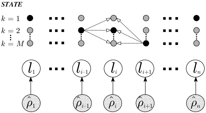
Figure 6.6.1: FCVB-marginals for HMC posterior (Fig. 6.4.1): trellis diagram (top) and DAG (bottom). Dotted arrows denote the CE substitutions in the Iterative FCVB algorithm. Black circles denote the mode of FCVB-marginal.

6.6.2.2 Further acceleration via a bubble-sort-like procedure

	ML	FCVB	VA	FB	VB
EXP	–	–	–	–	$O(nM\nu_{c})$
MUL	–	–	–	$O(2nM^{2})$	$O(2nM^{2}\nu_{c})$
ADD	–	$O(nM\nu_{c})$	$O(nM^{2})$	$O(2nM^{2})$	$O(2nM^{2}\nu_{c})$
MAX	$O(nM)$	$O(nM\nu_{c})$	$O(nM^{2})$	$O(nM)$	$O(nM)$
Memory	–	$O(n+M^{3})$	$O(nM)$	$O(2nM)$	$O(nM)$

Table 6.6.1: Computational and memory cost of algorithms for homogeneous HMC. $\nu_{c}$ is the number of IVB cycles at convergence (for accelerated scheme, $\nu_{c}$ is replaced by $\nu_{e}$). From the lowest to highest (typical) computational load: ML (Section 6.3.1), FCVB (Algorithm 6.9-6.10), VA (Algorithm 6.2), FB (Algorithm 6.1) and VB (Algorithm 6.7-6.8).

For comparing the computational complexity of above algorithms in the homogeneous HMC, a summary of their computational and memory cost is given in Table 6.6.1. Then, from Table 6.6.1, it looks like each FCVB cycle must be slower than ML, since each FCVB cycle seems to always require more operators than ML. In practice, however, each FCVB cycle can be implemented more quickly than ML. To achieve this, let us consider the computational load in hardware level.

The task of finding the maximum value of length-$M$ vector requires $M$ MAX operations, in which each MAX involves four steps (i-iv), as illustrated in Algorithm 6.11. Similarly, the task of finding the sum of a length-$M$ vector requires $M$ ADD operations, in which each ADD requires two steps (a-b), as illustrated in Algorithm 6.12. Hence, in practice, one MAX is often considered to be equivalent to $2$ ADDs [Wu (2001)]. In terms of computational load, if both maximum and sum are required, they can be computed more quickly via a Max-Sum combination, defined in Algorithm 6.14.

For further speed-up, notice that if the step (ii) in one MAX operation (Algorithm 6.11) does not detect any higher value than current maximum value, steps (iii) and (iv) will then not be implemented in that MAX operation. We can, therefore, design a pilot-based MAX scheme, which initializes the current maximum value with the pilot element in length-$M$ vector, as illustrated in Algorithm 6.13. The pilot element can be chosen as any of the $M$ vector elements. Therefore, in the ideal case where the pilot element is the true maximum, steps (iii)-(iv) can be avoided completely, i.e. the cost of pilot-based MAX (i.e. each iteration in Algorithm 6.15) can be as low as half of that of conventional MAX (i.e. each iteration in Algorithm 6.11). Likewise, in the ideal case, one pilot-MAX-ADD (i.e. each iteration in Algorithm 6.15) only needs three steps (i)-(ii)-(b), which means its cost is in the range $\eta\in\left[\frac{3}{4},\frac{5}{4}\right]$ of the cost of conventional MAX (in Algorithm 6.11).

Now, because each iterative FCVB cycle (6.6.5-6.6.6) involves Max-Sum scheme and ML requires traditional Max scheme, the considerations above can be applied to comparing the relative costs of FCVB and ML. Since the current FCVB cycle relies on the label estimates in the previous cycle, the latter can be used as pilot elements in current FCVB cycle. Therefore, the pilot-Max-Sum scheme (Algorithm 6.15) is applicable in FCVB cycles. In contrast, there is no scheme for picking pilot elements in ML, and therefore the ML has to rely on traditional Max scheme. For this reason, the cost of each pilot-based FCVB cycle is in the range $\eta\in\left[\frac{3}{4},\frac{5}{4}\right]$ of the cost of traditional ML, i.e. it is possible for each FCVB cycle to run faster than ML.

Notice that, the traditional MAX (Algorithm 6.11) is simply the first step in the bubble sort algorithm [Cormen et al. (2001)], in which the maximum value “floats” up progressively after each comparison step (ii). Then, the pilot-based MAX procedure above, which requires a priori knowledge on pilot element, can be loosely regarded as the first step of a pilot-based bubble sort, i.e. the maximum value will “float” up more quickly, given a good pilot element.

Obviously, we may have more than one way to make FCVB cycle run faster than ML. The above procedure is merely to illustrate such a possibility.

Initialization: set $k_{max}=1$, $k=1$ and $v_{max}=v_{1}$

Iteration:

(i) increase pointer by 1 (i.e. $k\leftarrow k+1$) and retrieve $v_{k}$

(ii) 1 binary comparison between $v_{max}$ and $v_{k}$

If $v_{\max}<v_{k}$ in (ii), do: {

(iii) 1 storage for new maximum value (i.e. $v_{max}\leftarrow v_{k}$)

(iv) 1 storage for position of new maximum value (i.e. $k_{max}\leftarrow k$) }

Termination: stop if $k=M$

Return: $v_{max}$ and $k_{max}$

Algorithm 6.11 Traditional Max for finding maximum $v_{max}$ of $v=[v_{1},\ldots,v_{M}]^{\prime}$

Initialization: set $v_{sum}=0$ and $k=1$

Iteration:

(a) increase pointer by 1 (i.e. $k\leftarrow k+1$) and retrieve $v_{k}$

(b) 1 binary addition $v_{sum}\leftarrow v_{sum}+v_{k}$

Termination: stop if $k=M$

Return: $v_{sum}$

Algorithm 6.12 Traditional Sum for finding sum $v_{sum}$ of $v=[v_{1},\ldots,v_{M}]^{\prime}$

Initialization: initialize $k_{pilot},$ set $k=1$, and $v_{max}=v_{k_{pilot}}$

Iteration:

Implement (i-iv) in Algorithm 6.11

Termination: stop if $k=M$

Return: $v_{max}$ and $k_{max}$

Algorithm 6.13 Pilot-based Max for finding maximum $v_{max}$ of $v=[v_{1},\ldots,v_{M}]^{\prime}$

Initialization: set $k_{max}=1$, $k=1$, $v_{max}=v_{1}$ and $v_{sum}=0$

Iteration:

Implement (i)-(ii)-(b)-(iii)-(iv) in Algorithm 6.11-6.12.

Termination: stop if $k=M$

Return: $v_{max}$, $k_{max}$ and $v_{sum}$

Algorithm 6.14 Max-Sum for finding maximum $v_{max}$ and sum $v_{sum}$ of $v=[v_{1},\ldots,v_{M}]^{\prime}$

Initialization: initialize $k_{pilot}$ and set $k=1$, $v_{max}=v_{k_{pilot}}$ and $v_{sum}=0$

Iteration:

Implement (i)-(ii)-(b)-(iii)-(iv) in Algorithm 6.11-6.12.

Termination: stop if $k=M$

Return: $v_{max}$, $k_{max}$ and $v_{sum}$

Algorithm 6.15 Pilot-based Max-Sum for finding maximum $v_{max}$ and sum $v_{sum}$ of $v=[v_{1},\ldots,v_{M}]^{\prime}$

6.7 Performance versus computational load

In this section, we will examine the trade-off between performance and computational costs for each of the algorithms above. For comparison of estimators performance, the bit-error-rate (BER) is widely adopted in practice [Haykin and Moher (2006)]. Since minimizing BER can also be interpreted as minimizing Hamming distance, the simulation results can be explained intuitively via the Bayesian risk perspective (Section 4.3.2).

6.7.1 Bayesian risk for HMC inference

Let us incorporate Hamming distance into a loss function $Q(\widehat{L_{n}},L_{n})$, that quantifies the cost of errors in the estimated HMC , $\widehat{l_{i}}\in\widehat{L_{n}}$, relative to the simulated field, $l_{i}\in L_{n}$, $i\in\{1,\ldots,n\}$, as follows:

$$Q(\widehat{L_{n}},L_{n})=1-\frac{1}{n}\sum_{i=1}^{n}\delta[\widehat{l_{i}}-l_{i}]$$

where $Q:\ M^{n}\times M^{n}\rightarrow[0,1]$ and $Q(\widehat{L_{n}},L_{n})=0\Leftrightarrow\widehat{L_{n}}=L_{n}$. As shown in Lemma 4.3.3, the estimate $\widehat{L_{n}*}$ minimizing expected loss - i.e. the minimum risk (MR) estimate - is:

$$\widehat{l_{i}^{*}}=\arg\max_{l_{i}}f(l_{i}|\mathbf{x}_{n})$$ (6.7.1)

where $\widehat{l_{i}^{*}}\in\widehat{L_{n}*}$, $i\in\{1,\ldots,n\}$. This MR risk provides insight into the observed trade-off in simulations (Chapter 8), as follows:

• FB can provide MR risk estimate $\widehat{L_{n}*}$ , being a sequence of marginal MAPs (6.7.1), where $f(l_{i}|\mathbf{x}_{n})$ are the smoothing marginals already computed in FB.

• The performance of VA is close to that of FB, with low computational load, for two reasons: VA replaces the marginal MAP of the smoothing marginals, $f(l_{i}|\mathbf{x}_{n})$, for FB with the MAP of the CE-based profile inferences, $f_{p}(l_{i}|\mathbf{x}_{n})$, with typically very little difference between these two estimates. However, the computational load of $f_{p}(l_{i}|\mathbf{x}_{n})$ is very low, compared to that of $f(l_{i}|\mathbf{x}_{n})$.

• ML yields the worst performance because it returns the estimates based on the local observation model, i.e. $\widehat{l_{i}}=\arg\max_{l_{i}}f(x_{i}|l_{i})$, without any prior regularization, i.e. $f(x_{i}|l_{i})$ is a bad approximation of $f(l_{i}|\mathbf{x}_{n})$ since it does not involve the HMC structure into account. However, the local observation structure makes ML work so fast.

An important role for the novel VB-approaches to HMC inference is in furnishing new trade-offs between computational load and accuracy, other than the extremes confined by ML on one hand, and FB and VA on the other. This flexibility is achieved via the following two design steps:

• In the first step, VB can return the MAP estimates of the respective VB-marginals, $\widehat{l_{i}}=\arg\max_{l_{i}}\widetilde{f}(l_{i}|\mathbf{x}_{n})$ (6.6.1). Since the VB-marginals are approximated via HMC-regularized model (6.2.2.1), this VB point estimate enjoys far better performance that that of ML.

• The second step is to reduce the complexity of VB via the CE approach in FCVB (6.6.5). Since the FCVB performance is slightly worse than VB, as illustrated in simulation (Chapter 8), its performance trade-off can be explained via VB’s structure.

6.7.2 Accelerated schemes

The number $\nu_{c}$ of IVB cycles in the HMC case will be shown, in simulations in Chapter 8, as a factor of logarithmic of either $n$, the number of data, or $M$, the number of state. We conjecture that this phenomenon is relevant to the exponential forgetting property of posterior marginals $f(l_{i}|\mathbf{x}_{n})$ (Corollary 2.1 in [Lember (2011)]):

$$||f(l_{i}|\mathbf{x}_{i-k:i+k})-f(l_{i}|\mathbf{x}_{-\infty:\infty})||\leq\frac{C}{\upsilon^{k-1}},\ k\geq 0$$ (6.7.2)

where $\upsilon$ is a constant, $\upsilon>1$, $C$ is a non-negative finite random variable, $\mathbf{x}_{-\infty:\infty}$ denotes an infinite number $n$ of data and $||\cdot||$ is the total variation distance (i.e. $\mathcal{L}_{1}$-norm). This property states that $f(l_{i}|\mathbf{x}_{n})$, with high enough $n$, only depends on a factor of $\log(n)$ data. Because each IVB-cycle updating in HMC (6.6.1) projects one more backward datum into the VB-marginals $\widetilde{f}(l_{i}|\mathbf{x}_{n})$, we conjecture that we only need a factor of $\log(n)$ IVB cycles in order for $\widetilde{f}(l_{i}|\mathbf{x}_{n})$ to converge, i.e. $\nu_{c}\approx O(\log(n))$.

For the accelerated schemes, $\nu_{c}$ is replaced by $\nu_{e}$, which we will find is almost a constant and close to $1$, on average, for any value of $n$ in simulations (Chapter 8). Hence, the accelerated scheme for FCVB and VB reduces significantly the computational load of traditional FCVB and VB for the HMC. Perhaps, this is because these schemes only update the non-converged VB-marginals, whose number decreases in a factor of $\log(n)$, owing to (6.7.2). This decrease is, therefore, likely to cancel out the $\nu_{c}\approx O(\log(n))$.

6.7.3 FCVB algorithm versus VA

By combining the CE approach with the independent class approximation, $f_{\delta}\in\mathcal{F}_{\delta}$, FCVB is faster than the non-iterative VA scheme, despite FCVB being an iterative scheme. From Table 6.6.1, we can see that FCVB reduces the computational load from $O(nM^{2})$ for VA down to $O(nM\nu_{c})$. Hence, the computational load of VA increases quadratically with $M$, while FCVB’s computational load increases only linearly with $M$. Moreover, from simulations (Chapter 8) for FCVB, it will be shown that $\nu_{e}\ll\nu_{c}\approx O(\log(M))$ when $M$ is large.

A key advantage of the FCVB scheme is applicability in many practical applications. Note that, VA is mostly applied to finite state HMC, because the conditional CE (6.3.6) is very hard to evaluate for continuous states, other than in the Gaussian context of the Kalman filter [Chigansky and Ritov (2011)]. In contrast, since Iterative FCVB algorithm is equivalent to the ICM algorithm [Besag (1986)], with application in the general Hidden Markov Model (HMM) context, the Accelerated FCVB - a faster version of ICM - can also be applied feasibly to the continuous state case.

Another application of VB and FCVB for the HMC is the online context. Because VB-marginals only depend on their first order neighbour in (6.6.3) and (6.6.5), the VB-marginal updates in IVB cycles can be run consecutively and in parallel, i.e. $\widetilde{f}^{[\nu]}(l_{i-1}|\mathbf{x}_{n})$ can be updated right after $\widetilde{f}^{[\nu-1]}(l_{i}|\mathbf{x}_{n})$ is updated, without the need to wait for the $(\nu-1)$th IVB cycle to be finished. If we design a lag-window of duration equal to $\nu_{c}$, the $\nu_{c}$ FCVB and VB cycles can be evaluated, consecutively and in parallel, as an online algorithm and return exactly the same results as the offline case.

6.8 Summary

In this chapter, fully Bayesian inference and its computation for the HMC has been developped, revealing a key insight into all of the state-of-the-art algorithms, namely FB, VA and ICM; i.e. the Markov property of the HMC has been shown to be a necessary foundation for their efficient recursive computational flow. In replacing the exact marginal computations in FB algorithm, the VA has been shown to produce CE-based approximate inferences, where CE substitution is used to reduce the computational load significantly. Importantly, the joint MAP estimate remains invariant under this CE substitution.

Inspired by this insight, FCVB, which is a CE-based variant of the independent-structure VB approximation, has been proposed as a VA variant to bridge the trade-off gap between VA and ML. Although FCVB has previously been reported as the ICM algorithm in the literature, this novel VB-based derivation and implementation yields insight into the regimes of operation where the algorithm is expected to perform well. Indeed, we will see in simulations in Chapter 8 that when correlation in the HMC is not too high, FCVB is an attractive algorithm, since its performance is then close to VA, with much lower computational load. Empirically, these simulations also show that the accelerated scheme, as designed in this chapter, reduces the number of IVB cycles to about one, on average.

Finally, the accelerated ICM/FCVB algorithm—proposed in this chapter—can work in both online and offline modes, with no difference at the final output, as noted in Section 6.7.3. In contrast, FB and VA are exclusively the offline schemes.

Chapter 7 The transformed Variational Bayes (TVB) approximation

7.1 Motivation

Although the VB approximation has been proposed as an efficient approximation for intractable distributions, there is still much room for improvement.

The VB approximation is, of course, a parametric distribution, $f_{\theta}\triangleq f(\theta|s)$, where $s$ denotes the parameter. For simplicity, let us consider a binary partition $\theta=\{\theta_{i},\theta_{\backslash i}\}$, where, again, $\theta_{\backslash i}$ is the complement set of $\theta_{i}$ in $\theta$, with neither $\theta_{\backslash i}$ nor $\theta_{i}$ is empty. As explained in Section 4.5.2, the VB approximation reaches a local minimum of Kullback-Leibler divergence $KLD(\tilde{f}_{\theta}||f_{\theta})=E_{\tilde{f}_{\theta}}\log(\tilde{f}_{\theta}/f_{\theta})$, for approximate distributions $\widetilde{f}_{\theta}\in\mathcal{F}_{c}$, the class of factored distributions (being those for which $\theta_{\backslash i}$ and $\theta_{i}$ are independent, given $s$).

The idea behind the transformed VB (TVB) approximation is illustrated in Fig. 7.1.1. The transformed distribution $f_{\phi}\triangleq f(\phi|s^{\prime})$, with parameter $s^{\prime}$ (a function of $s$), should be designed to minimize the $KLD$ of its VB approximation. Since $KLD(\tilde{f}_{\phi}||f_{\phi})<KLD(\tilde{f}_{\theta}||f_{\theta})$, it follows that $KLD(\tilde{f}_{\theta}^{TVB}||f_{\theta})<KLD(\tilde{f}_{\theta}||f_{\theta})$.

Obviously, VB yields an accurate representation, i.e. $KLD(\tilde{f}_{\theta}||f_{\theta})=0$, iff $\theta_{i}$, $\theta_{\backslash i}$ are already independent in $f_{\theta}$. An illustrative context is the multivariate normal distribution ${\cal N}_{\theta}(0,\Sigma)$. The $KLD$ of its VB approximation is strictly greater than zero when $\Sigma\neq D$ (diagonal). Let us consider a rotation operator via eigenvectors of the covariance matrix, i.e. $\phi=Q^{-1}\theta$, where $\Sigma^{-1}=Q\Lambda Q^{-1}$ and $\Lambda$ is the diagonal eigenvalue matrix. The distribution of transformed variables $\phi$ is the independent multivariate normal $N_{\phi}\left(0,\Lambda\right)$, and the VB approximation in this transformed metric has $KLD(\tilde{f}_{\phi}||f_{\phi})=0$.

Figure 7.1.1: Transformed VB (top) and VB (below) approximations. $T$ denotes a bijective transformation, $T:\theta\rightarrow T(\theta)=\phi$.

Transformed VB (top) with orthogonalization and VB (below) approximations for the multivariate normal distribution.

7.2 Transformed VB approximation

In the literature, Cox-Reid orthogonalization [Cox and Reid (1987)] has been applied broadly to parameter estimation to achieve robustness, yet very few paper consider this approach for Bayesian inference. Based on the Fisher information matrix, its approach is to decouple a joint distribution up to second order. A slightly more general transformation will be proposed in this section in order to increase the quality of the VB approximation.

7.2.1 Distributional transformation

Let us consider a distribution $f(\theta)$ of continuous r.v. $\theta$. Then, given a bijective mapping $\phi=g\left(\theta\right)$, we can derive the distribution $f(\phi)$ of continuous r.v. $\phi$, as follows [Freeman (1963); Arnold (2009)]:

$$f(\phi)=\left.\frac{f(\theta)}{J(\theta)}\right|_{\theta=g^{-1}(\phi)}$$

where $J(\theta)\triangleq\left|\det\left(\frac{d\phi}{d\theta}\right)\right|$ is the Jacobian determinant of the transformation, $\phi=g\left(\theta\right)$, and $\left|\cdot\right|$ denotes magnitude.

7.2.2 Locally diagonal Hessian

As presented in Section 4.4.3.4, let us consider the negative logarithm of the transformed distribution $L(\phi)\triangleq\log f(\phi)$, expanded up to the second order of the Taylor approximation at a point $\phi_{0}$ at which $L(\phi)$ is infinitely differentiable, as follows:

$$L(\phi)=L(\phi_{0})+(\phi-\phi_{0})^{\prime}\nabla L(\phi_{0})-\frac{1}{2}(\phi-\phi_{0})^{\prime}H(\phi_{0})(\phi-\phi_{0})+\ldots$$

where $\nabla L(\phi_{0})$ and $H(\phi_{0})\triangleq-\nabla^{2}L(\phi_{0})$ are gradient vector and Hessian matrix, respectively, evaluated at $\phi_{0}$. In contrast to the Fisher information matrix approach in [Cox and Reid (1987)], we propose to design the transformation, $g(\cdot)$, in order to diagonalize the Hessian matrix. Its insight is, actually, a quadratic decoupling up to second order, which yields the asymptotic independence (see Proposition 4.4.5).

Such a transformation can be designed via matrix decomposition. The transformed Hessian, $H(\phi)$, is desired to be diagonal locally at $\phi=\phi_{0}=g(\theta_{0})$, in which a specific value $\theta_{0}$ can be chosen freely, typically a certainty equivalent (CE) such as mean, mode, etc. For this purpose, a linear transformation matrix $A$ can be defined such that $g(\theta)=A\theta$, where $A$ is an invertible matrix. The Jacobian of matrix transformation is also feasible to compute in this case: $J(\theta)=\det(A)$, a constant. We consider two designs for $A$, as follows:

• Method$(I)$ - Eigen decomposition: Let $A=Q^{-1}$, where $H(\theta_{0})=Q\Lambda Q^{-1}$ in the original (untransformed) metric. Then, the Hessian in the transformed metric is $H(\phi_{0})=\Lambda$, $\forall\phi_{0}\in\Phi$, becomes diagonal at $\phi_{0}$ and $J(\theta)=\det(Q^{-1})=1$.

• Method$(II)$ - LDU decomposition: Let $A=U$, where $H(\theta_{0})=LDU$, and $L=U^{\prime}$ is a lower triangular matrix with unit diagonal. Then, transformed Hessian $H(\phi_{0})=D$ is diagonal by design, $\forall\phi_{0}\in\Phi$, and $J(\theta)=\det(U)=1$.

While the Eigen decomposition is easier to implement in practice, the LDU decomposition has one advantage: the variable corresponding to the last row of $A=U$ is kept unchanged.

7.3 Spherical distribution family

The spherical distribution refers to the family of distributions that are closed under any diagonalization transformation [Kelker (1970)]. Recently, in Bayesian analysis, it has been shown to be an observation model, whose conjugate prior is the so-called dispersion elliptical squared-radial (DESR) distribution - an extension of normal-gamma family [Arellano-Valle et al. (2006)]. The form of spherical distribution is defined as

$$f(\theta|\mu,\Sigma)\propto\left|\Sigma\right|^{-\frac{1}{2}}\psi(u(\theta))$$ (7.3.1)

where $\mu$ is the mean vector and $\Sigma$ is the covariance matrix for $\theta$, $\psi$ is a function satisfying the normalizing condition for $f(\theta|\mu,\Sigma)$ and

$$u(\theta)=(\theta-\mu)^{\prime}\Sigma^{-1}(\theta-\mu)$$ (7.3.2)

is the quadratic form implied by $\mu$ and $\Sigma$.

Let us, once again, denote $L(\theta)\triangleq-\log f(\theta)$. Then, by the chain rule for the composite functions, its Hessian matrix can be derived, as follows:

$$H(\theta)=-\nabla^{2}L(\theta) =-\frac{\partial^{2}L(\theta)}{\partial u^{2}}\nabla u(\theta)\nabla u\left(\theta\right)^{\prime}-\frac{\partial L(\theta)}{\partial u}\nabla^{2}u(\theta)$$

$$=-\frac{\partial^{2}L(\theta)}{\partial u^{2}}\Sigma^{-1}(\theta-\mu)(\theta-\mu)^{\prime}\Sigma^{-1}-\frac{\partial L(\theta)}{\partial u}\Sigma^{-1}$$ (7.3.3)

7.3.1 Multivariate Normal distribution

Since the first term in (7.3.3) is zero at the mean $\mu$, and $\Sigma^{-1}$ in the second term is diagonalizable, $H(\phi_{0})$ can be locally diagonalized at the mean $\theta_{0}=\mu$ for any spherical distribution via the local diagonalization methods (I) and (II). In particular, $H(\phi_{0})$ is globally diagonal in the multivariate normal distribution, since, for this choice of linear transformations, we have $\frac{\partial^{2}L(\theta)}{\partial u^{2}}=0$, $\forall\theta\in\Theta$. This corresponds to our setting in Section 7.1.

7.3.2 Bivariate power exponential (PE) distribution

Let us study another illustrative example for this spherical family (7.3.1), namely bivariate power exponential (PE) distribution, defined as follows [Gomez et al. (1998)]:

$$f(\theta|\mu,\Sigma) =\frac{\sqrt{2}}{\pi\sqrt{\pi}}\left|\Sigma\right|^{-\frac{1}{2}}\exp\left(-\frac{1}{2}u(\theta)^{2}\right)$$ (7.3.4)

where $\theta\in\mathbb{R}^{2}$ and $u(\theta)$ is given in (7.3.2). Because it is difficult to express two true marginals in closed form [Gomez et al. (2008)], let us study the VB approximation for bivariate PE distribution next.

7.3.2.1 VB approximation for bivariate PE

Without loss of generality, let us assume that $\mu=0$ in the sequel. Hence, we can write $f(\theta|\Sigma)\triangleq f(\theta|\mu=0,\Sigma)$, where $\Sigma\triangleq\left[\begin{array}[]{cc}\sigma_{1}^{2}&\rho\sigma_{1}\sigma_{2}\\ \rho\sigma_{1}\sigma_{2}&\sigma_{2}^{2}\end{array}\right]$ and $\rho$ is the correlation coefficient. At cycle $\nu$, the VB-marginals (Theorem 4.5.1) for (7.3.4) can be computed as follows:

$$\tilde{f}^{[\nu]}(\theta_{i}) \propto \exp\left(E_{\tilde{f}^{[\nu-1]}(\theta_{\backslash i})}\log f(\theta|\Sigma)\right),\hskip 10.00002pti\in\{1,2\}$$

$$\propto \exp\left(-\frac{1}{2}E_{\tilde{f}^{[\nu-1]}(\theta_{\backslash i})}\left(\theta^{\prime}\Sigma^{-1}\theta\right)^{2}\right)$$

$$\propto \exp\left(-\frac{1}{2\left(1-\rho^{2}\right)^{2}}\sum_{k=1}^{4}\alpha_{i,k}\theta_{i}^{k}\right)$$

where eight VB shaping parameters $\alpha_{i,k}$ are:

$$\begin{cases}\alpha_{i,4}&=\frac{1}{\sigma_{i}^{4}}\\ \alpha_{i,3}&=-\frac{4\rho}{\sigma_{i}^{3}\sigma_{\backslash i}}\left[\widehat{\theta_{\backslash i}}\right]\\ \alpha_{i,2}&=\frac{2(1-\rho^{2})}{\sigma_{i}^{2}\sigma_{\backslash i}^{2}}\left[\widehat{\theta_{\backslash i}^{2}}\right]\\ \alpha_{i,1}&=-\frac{4\rho}{\sigma_{i}\sigma_{\backslash i}^{3}}\left[\widehat{\theta_{\backslash i}^{3}}\right]\end{cases}$$

with $\widehat{\theta_{\backslash i}}$, $\widehat{\theta_{\backslash i}^{2}}$ and $\widehat{\theta_{\backslash i}^{3}}$ denoting first, second and third VB moments of $\theta_{\backslash i}$, i.e with respect to $\tilde{f}^{[\nu-1]}(\theta_{\backslash i})$.

7.3.2.2 TVB approximation for bivariate PE

The transformed distribution of $\phi=A\theta$ are designed as $A=Q^{-1}$ , where $\Sigma^{-1}=Q\Lambda Q^{-1}$ for (I) and $A=U$, where $\Sigma^{-1}=LDU$ for (II).

For conciseness, only the case (I) is presented below, with similar findings for the case (II). The transformed distribution of $\phi=A\theta$ under (I) is:

$$f(\phi|\Lambda) \propto \left|\Sigma\right|^{-\frac{1}{2}}\exp\left[-\frac{1}{2}\left(\phi^{\prime}\Lambda^{-1}\phi\right)^{2}\right]$$

The VB approximations are derived as follows:

$$\tilde{f}^{[\nu]}(\phi_{i}) \propto \exp\left(E_{\tilde{f}^{[\nu-1]}(\phi_{\backslash i})}\log f(\phi|\Lambda)\right),\ i\in\{1,2\}$$

$$\propto \exp\left(-\frac{1}{2}E_{\tilde{f}^{[\nu-1]}(\theta_{\backslash i})}\left(\phi^{\prime}\Lambda\phi\right)^{2}\right)$$

$$\propto \exp\left(-\frac{1}{2}\left(\lambda_{i}\phi_{i}^{2}+\lambda_{\backslash i}\left[\widehat{\phi_{\backslash i}^{2}}\right]\right)^{2}\right)$$

where $\lambda_{i}$,$\lambda_{\backslash i}$ are the two eigenvalues of $\Sigma^{-1}$ (i.e. the diagonal elements of $\Lambda$) and $\widehat{\phi_{\backslash i}^{2}}$ is the second moment of $\phi$ with respect to $\tilde{f}^{[\nu-1]}(\phi_{\backslash i})$. At convergence, the VB approximation for the transformed $f(\phi|\Lambda)$ distribution are:

$$\widetilde{f}(\phi|\Lambda) = \widetilde{f}(\phi_{1}|\Lambda)\widetilde{f}(\phi_{2}|\Lambda)$$

$$\propto \exp\left(-\frac{1}{2}\left[\left(\lambda_{1}\phi_{1}^{2}+\lambda_{2}\left[\widehat{\phi_{2}^{2}}\right]\right)^{2}+\left(\lambda_{2}\phi_{2}^{2}+\lambda_{1}\left[\widehat{\phi_{1}^{2}}\right]\right)^{2}\right]\right)$$

Substituting $\phi=Q^{-1}\theta$ into $\widetilde{f}(\phi|\Lambda)$, we will retrieve the TVB approximation of $f(\theta|\Sigma)$, i.e. $\tilde{f}_{TVB}(\theta|\Sigma)$: Also, the normalizing constant can be evaluated numerically.

7.3.2.3 Contour plot

The results for $\mu=[2.5,1]^{T}$, $\sigma_{1}=0.5$, $\sigma_{2}=1.5$ and various correlation coefficients, $\rho\in(0,1)$, are shown in Fig. 7.3.1 and Fig. 7.3.2. In Fig. 7.3.2, we can see that the $KLD$ of TVB approximation is equal to its minimum value of original VB and becomes invariant with $\rho$ owing to diagonalization methods. Although the relationship between (I) and (II) is not expressed explicitly, the coincide $KLD$ values show that they seem to be equivalent to each other.

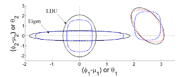
Figure 7.3.1: Bivariate PE distribution and its approximations ($\rho=-0.5$). On the right: $f_{\theta},$ $\tilde{f}_{\theta}^{VB}$, $\tilde{f}_{\theta}^{TVB}$ are denoted by $(-,\ -.\ ,\ :\ )$ respectively; on the left: $f_{\phi}$ and $\tilde{f}_{\phi}$ are denoted by $(-,\ -.\ )$ respectively. For clarity, the VB and TVB approximations are shifted to the origin in that figure.

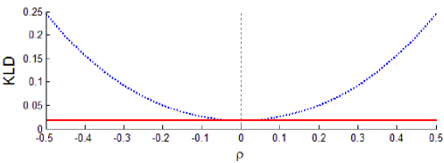
Figure 7.3.2: KLD of VB (above, dotted line) and TVB for bivariate PE distribution

7.4 Frequency inference in the single-tone sinusoidal model in AWGN

In this section, the Bayesian inference for single-tone frequency will be illustrated. Despite being simple, this canonical model in digital receivers is non-linear with frequency and, hence, intractable for frequency’s posterior computation. The performance of two posterior’s approximations, VB and TVB, will also be compared and illustrated.

Based on receiver’s model in equation (3.2), let us consider a received sinusoidal sequence $\mathbf{x}_{n}\triangleq[x_{1},\ldots,x_{n}]^{\prime}$ over the AWGN channel:

$$x_{i}=a\sin(\Omega i)+z_{i},\ i\in\{1,\ldots,n\}$$ (7.4.1)

where $z_{i}\overset{i.i.d}{\sim}\mathcal{N}(0,r_{e})$. The observed sequence (7.4.1) can be written in vector form, as follows:

$$\mathbf{x}_{n}=a\mathbf{g}_{n}+\mathbf{z}_{n},\ i\in\{1,\ldots,n\}$$ (7.4.2)

where $\mathbf{z}_{n}\triangleq[z_{1},\ldots,z_{n}]^{\prime}$ is the vector of noise samples, and $\mathbf{g}_{n}\triangleq[\sin(\Omega 1),\ldots,\sin(\Omega n)]^{\prime}$ is the vector of regression function. The implied observation distribution is:

$$f(\mathbf{x}_{n}|a,\Omega) = \prod_{i=1}^{n}\mathcal{N}_{x_{i}}\left(a\sin(\Omega i),r_{e}\right)$$

$$= \mathcal{N}_{\mathbf{x}_{n}}\left(a\mathbf{g}_{n},r_{e}\mathbf{I}\right)$$

where $\mathbf{I}$ is the identity matrix. For prior knowledge, $\Omega$ is chosen as uniform over $[0,\pi)$ (rad/sample) a priori. For amplitude $a$, the conjugate prior in this sinusoidal model is $f(a)=\mathcal{N}_{a}\left(\mu_{a},r_{a}\right)$. This conjugacy was noted in [Bromberg and Progri (2005)] and elsewhere.

7.4.1 Joint posterior distribution

The joint posterior for $\{a,\Omega\}$ can be derived as follows:

$$f(a,\Omega|\mathbf{x}_{n}) \propto \prod_{i=1}^{n}\mathcal{N}_{x_{i}}\left(a\sin(\Omega i),r_{e}\right)\mathcal{N}_{a}\left(\mu_{a},r_{a}\right)$$ (7.4.3)

$$\propto \exp\left(-\frac{a^{2}\left(\frac{1}{r(\Omega)}\right)-2\mu\left(\Omega\right)\frac{1}{r(\Omega)}a}{2}\right)$$

$$\propto \mathcal{N}_{a}\left(\mu\left(\Omega\right),r(\Omega)\right)\exp\left(\frac{\mu\left(\Omega\right)^{2}}{2r(\Omega)}\right)\sqrt{2\pi r(\Omega)}$$ (7.4.4)

in which:

$$\frac{1}{r(\Omega)} \triangleq \frac{\sum_{i=1}^{N}\sin^{2}(\Omega i)}{r_{e}}+\frac{1}{r_{a}}$$

$$= \frac{\left\|\mathbf{g}_{n}\right\|^{2}}{r_{e}}+\frac{1}{r_{a}}$$

$$\mu\left(\Omega\right) \triangleq r(\Omega)\left(\frac{\sum_{i=1}^{N}x_{i}\sin(\Omega i)}{r_{e}}+\frac{\mu_{a}}{r_{a}}\right)$$ (7.4.6)

$$= \frac{\frac{X_{I}(e^{j\Omega})}{r_{e}}+\frac{\mu_{a}}{r_{a}}}{\frac{\left\|\mathbf{g}_{n}\right\|^{2}}{r_{e}}+\frac{1}{r_{a}}}$$

expressed in term of $X_{I}(e^{j\Omega})\triangleq Im\{X(e^{j\Omega})\}=\mathbf{x}_{n}^{\prime}\mathbf{g}_{n}$ and in term of $\left\|\mathbf{g}_{n}\right\|=\mathbf{g}_{n}^{\prime}\mathbf{g}_{n}$ .

From (7.4.4), we can see that Gaussian form is preserved for $f(a|\Omega,\mathbf{x}_{n})=\mathcal{N}_{a}(\mu\left(\Omega\right),$ $r(\Omega))$, owing to the conjugate prior $f(a)=\mathcal{N}_{a}\left(\mu_{a},r_{a}\right)$ defined above, and the marginal distribution for $\Omega$ can be expressed in closed form as:

$$f(\Omega|\mathbf{x}_{n})\propto\exp\left(\frac{\mu\left(\Omega\right)^{2}}{2r(\Omega)}\right)\sqrt{r(\Omega)}$$ (7.4.7)

However, the distribution (7.4.7) is non-standard and intractable in $\Omega$, owing to the nonlinear dependence on $\Omega$, a result that is widely known [Rife and Boorstyn (1974); Quinn (1992)]. This sinusoidal model is therefore a canonical candidate for distributional approximation.

For later use, let us compute joint MAP estimate $\{\widehat{a},\widehat{\Omega}\}$. From (7.4.4), we can see feasibly that $\widehat{a}=\mu\left(\widehat{\Omega}\right)$ and, by substituting that $\widehat{a}$ to $\mathcal{N}_{a}\left(\mu\left(\Omega\right),r(\Omega)\right)$in (7.4.4), we have:

$$\widehat{\Omega} = \arg\max_{\Omega}\exp\left(\frac{\mu\left(\Omega\right)^{2}}{2r(\Omega)}\right)$$

$$= \arg\max_{\Omega}\frac{\left(\frac{X_{I}(e^{j\Omega})}{r_{e}}+\frac{\mu_{a}}{r_{a}}\right)^{2}}{2\left(\frac{\left\|\mathbf{g}_{n}\right\|^{2}}{r_{e}}+\frac{1}{r_{a}}\right)}$$

7.4.2 VB approximation

From (7.4.3), the VB approximation (Theorem 4.5.1) for $f(a,\Omega|\mathbf{x}_{n})$ is (Fig. 7.1.1):

$$\widetilde{f}_{VB}(a,\Omega|\mathbf{x}_{n}) = \widetilde{f}_{VB}(a|\mathbf{x}_{n})\widetilde{f}_{VB}(\Omega|\mathbf{x}_{n})$$

$$\propto \mathcal{N}_{a}\left(\mu_{1},\sigma_{1}^{2}\right)\exp\left(\frac{\alpha_{1}\mu\left(\Omega\right)+\alpha_{2}}{2r(\Omega)}\right)$$

in which the iterative VB’s shaping parameters are:

$$\mu_{1} = E_{\widetilde{f}_{VB}(\Omega|\mathbf{x}_{n})}\left[\mu\left(\Omega\right)\right]$$ (7.4.9)

$$\sigma_{1}^{2} = E_{\widetilde{f}_{VB}(\Omega|\mathbf{x}_{n})}\left[r(\Omega)\right]$$

$$\alpha_{1} = E_{\widetilde{f}_{VB}(a|\mathbf{x}_{n})}\left[2a\right]=2\mu_{1}$$

$$\alpha_{2} = E_{\widetilde{f}_{VB}(a|\mathbf{x}_{n})}\left[-a^{2}\right]=-(\mu_{1}^{2}+\sigma_{1}^{2})$$

with $\widetilde{f}_{VB}(\Omega|\mathbf{x}_{n})\propto\exp\left(\frac{\alpha_{1}\mu\left(\Omega\right)+\alpha_{2}}{2r(\Omega)}\right)$ and $\widetilde{f}_{VB}(a|\mathbf{x}_{n})=\mathcal{N}_{a}\left(\mu_{1},\sigma_{1}^{2}\right)$.

7.4.3 TVB approximation

The TVB approximation via LDU diagonalization (i.e. Method (II) in Section 7.2.2) will be considered next.

Because the Hessian matrix in this case is a symmetric $2\times 2$ matrix, the upper off-diagonal element $u_{12}$ in matrix $U$ of LDU decomposition for Hessian matrix is $u_{12}=H_{12}/H_{11}=r(\Omega)\left(\sum_{i=1}^{n}\frac{2i\cos(\Omega i)\left(x_{i}-2a\sin(\Omega i)\right)}{r_{e}}\right)$, where $H_{11}\triangleq-\frac{\partial^{2}\log f(a,\Omega|\mathbf{x}_{n})}{\partial a^{2}}$ and $H_{12}\triangleq-\frac{\partial^{2}\log f(a,\Omega|\mathbf{x}_{n})}{\partial a\partial\Omega}$. The transformed variable $[\lambda,\Omega]^{\prime}=U[a,\Omega]^{\prime}$ in this case is:

$$\lambda=a+\widehat{u}_{12}\Omega$$ (7.4.10)

where $\widehat{u}_{12}$ denotes $u_{12}$ evaluated at joint MAP estimate $\{\widehat{a},\widehat{\Omega}\}$.

Note that, the Jacobian in the LDU transformation is always unity, i.e. $\det(U)=1$, as explained in Section 7.2.2. Then, by changing $a$ to $\lambda$, the transformed distribution is $f(\lambda,\Omega|\mathbf{x}_{n})=\left.f(a,\Omega|\mathbf{x}_{n})\right|_{a=\lambda-\widehat{u}_{12}\Omega}$ and the VB approximation (Theorem 4.5.1) for $f(\lambda,\Omega|\mathbf{x}_{n})$ is (Fig. 7.1.1):

$$\widetilde{f}(\lambda,\Omega|\mathbf{x}_{n}) = \widetilde{f}(\lambda|\mathbf{x}_{n})\widetilde{f}(\Omega|\mathbf{x}_{n})$$

$$\propto \mathcal{N}_{\lambda}\left(\mu_{2},\sigma_{2}^{2}\right)\exp\left(\frac{\beta_{1}\mu_{0}\left(\Omega\right)+\beta_{2}}{2r(\Omega)}\right)\exp\left(\frac{\mu^{2}\left(\Omega\right)-\mu_{0}^{2}\left(\Omega\right)}{2r(\Omega)}\right)$$

in which:

$$\mu_{0}\left(\Omega\right)\triangleq\mu\left(\Omega\right)+u_{12}\Omega$$

and the iterative VB’s shaping parameters are:

$$\mu_{2} = E_{\widetilde{f}(\Omega|\mathbf{x}_{n})}\left[\mu\left(\Omega\right)\right]$$ (7.4.12)

$$\sigma_{2}^{2} = E_{\widetilde{f}(\Omega|\mathbf{x}_{n})}\left[r(\Omega)\right]$$

$$\beta_{1} = E_{\widetilde{f}(\lambda|\mathbf{x}_{n})}\left[2\lambda\right]=2\mu_{2}$$

$$\beta_{2} = E_{\widetilde{f}(\lambda|\mathbf{x}_{n})}\left[-\lambda^{2}\right]=-(\mu_{2}^{2}+\sigma_{2}^{2})$$

with $\widetilde{f}(\Omega|\mathbf{x}_{n})\propto\exp\left(\frac{\beta_{1}+\beta_{2}\mu_{0}\left(\Omega\right)}{2r(\Omega)}+\frac{\mu^{2}\left(\Omega\right)-\mu_{0}^{2}\left(\Omega\right)}{2r(\Omega)}\right)$ and $\widetilde{f}(\lambda|\mathbf{x}_{n})=\mathcal{N}_{\lambda}\left(\mu_{2},\sigma_{2}^{2}\right)$.

Note that, the Jacobian in inverse LDU transformation is, once again, unity. By applying the inverse transformation, i.e. $a=\lambda-\widehat{u}_{12}\Omega$ (from (7.4.10)), the TVB approximation for $f(a,\Omega|\mathbf{x}_{n})$ is $\left.\widetilde{f}(\lambda,\Omega|\mathbf{x}_{n})\right|_{\lambda=a+\widehat{u}_{12}\Omega}$, i.e. (Fig. 7.1.1):

$$\widetilde{f}_{TVB}(a,\Omega|\mathbf{x}_{n}) = \widetilde{f}_{TVB}(a|\Omega,\mathbf{x}_{n})\widetilde{f}_{TVB}(\Omega|\mathbf{x}_{n})$$

$$= \mathcal{N}_{a}\left(\mu_{2}-\widehat{u}_{12}\Omega,\sigma_{2}^{2}\right)\widetilde{f}(\Omega|\mathbf{x}_{n})$$

where $\widetilde{f}_{TVB}(\Omega|\mathbf{x}_{n})=\widetilde{f}(\Omega|\mathbf{x}_{n})$, defined in (7.4.3).

Comparing TVB approximations (7.4.3) with VB (7.4.2) , we can see that the two factors in TVB are not independent anymore like those in VB, owing to linearization (7.4.10) at specific point $\{a,\Omega\}$ in coefficient $u_{12}$. This result shows that TVB is, in this case, a non-naive mean field approximation.

Remark 7.4.1.

Note the similarity between $\widetilde{f}_{VB}(\Omega|\mathbf{x}_{n})$ in (7.4.2) and $\widetilde{f}_{TVB}(\Omega|\mathbf{x}_{n})=\widetilde{f}(\Omega|\mathbf{x}_{n})$ in (7.4.3,7.4.3), whose key difference is the extra factor $\exp\left(\frac{\mu^{2}\left(\Omega\right)-\mu_{0}^{2}\left(\Omega\right)}{2r(\Omega)}\right)$. Because this extra factor involves the second order $\mu^{2}\left(\Omega\right)$ like the true marginal $f(\Omega|\mathbf{x}_{n})$ in (7.4.4), the frequency estimation of TVB is expected to be better than that of VB, which only takes into account the first order $\mu\left(\Omega\right)$.

7.4.4 Simulation

All iterative shaping parameters, $\mu$, $\sigma$, $\alpha$, $\beta$ in (7.4.9, 7.4.12) are evaluated numerically at DFT-bins of $\Omega$. The performance of $\Omega$ estimators for various schemes is shown in Fig. 7.4.1. Here, $n=1024$ and $\Omega=1.1$ DFT-bins, i.e. $\Omega=1.1\frac{2\pi}{n}$ rad/sample. The value 1.1 was chosen so that the true digital frequency $\Omega$ is always off-bin, no matter how high the resolution of the DFT-bin quantization is. Also, the fact that $\Omega$ is close to one represents a stressful regime for the $\Omega$ estimator [Rife and Boorstyn (1974); Quinn (1992)]. The SNR is $SNR=\frac{\mu_{a}^{2}+r_{a}}{2r_{e}}$, where the prior parameters were chosen as $\mu_{a}=1$ and $r_{a}=0.1$, representing small variance of normalized attenuation. The number of Monte Carlo runs is $10^{6}$.

7.4.4.1 Performance of frequency estimates

Because the loss function is the root mean square (RMS) error, the posterior mean $\widehat{\Omega}_{MEAN}$ is the minimum-risk estimator (4.3.6), as verified in Fig. 7.4.1. Owing to prior information, the joint MAP $\widehat{\Omega}_{MAP}$ estimator is slightly better than joint ML $\widehat{\Omega}_{ML}$ . However, because both of them can only detect the frequency at DFT-bins, they are much worse than $\widehat{\Omega}_{MEAN}$ in this off-bin case.

For illustration of the VB schemes. both VB $\widehat{\Omega}_{VB}$ and TVB $\widehat{\Omega}_{TVB}$ estimators are chosen as the mean of $\widetilde{f}_{VB}(\Omega|\mathbf{x}_{n})$ and $\widetilde{f}_{TVB}(\Omega|\mathbf{x}_{n})$, respectively. Because the joint distribution of $\Omega$ concentrates around single point at high SNR, the performance of a naive mean field approximation like VB does increase but is still not good in this case. In contrast, the performance of the TVB estimator is much higher and close to joint MAP performance, owing to its linearization around $\widehat{\Omega}_{MAP}$.

7.4.4.2 Evaluation of computational load via FFT

Since FFT algorithm was applied to all schemes, their computational load was of the same efficient order $O(n\log n)$. Note that, owing to the asymptotic nature of $O(\cdot)$, we do not consider the difference of a factor $O(1)$ in the computational load of the schemes above. In practice, iterative schemes such as VB and TVB may be $\nu$-times slower than a standard FFT-based scheme such as ML, where $\nu$ is the number of iterations at convergence. The number of iteration $\nu$ for VB and TVB was fixed at $5$, since no increase in performance was visible for higher $\nu$.

Owing to FFT, the Bayesian posterior inference $\widehat{\Omega}_{MEAN}$ yields a good trade-off scheme, i.e. small loss in speed but high gain in performance, compared to ML estimator via periodogram. However, the iterative VB and TVB methods, although being $\nu$ times slower than Bayesian scheme, do not yield better performance than $\widehat{\Omega}_{ML}.$ or $\widehat{\Omega}_{MAP}.$ Hence, although they cannot be recommended for this single-tone problem, the simulation has verified the superiority of TVB to VB method, which is the main motivation of designing TVB.

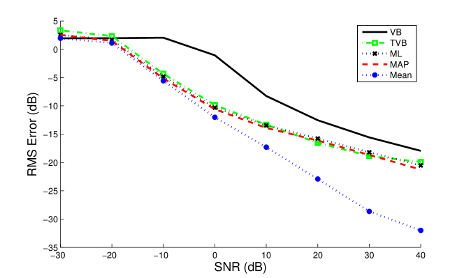
Figure 7.4.1: Root mean square (RMS) error in estimation of $\Omega=1.1$ DFT-bins for the single-tone sinusoidal AWGN, via conventional methods and via VB variants

7.5 Summary

This chapter began with an illustrative example, which showed that rotation can render independent (i.e.  decouple) bivariate Gaussian random variables and, hence, reduce the Kullback-Leibler divergence (KLD) in the VB approximation to zero. This idea encouraged us to design the rotation via the transformed Hessian matrix in any posterior distribution at a desired CE point, with the VB approximation then being performed in the transformed metric. This novel scheme was defined as transformed VB (TVB) approximation. Thanks to the asymptotic independence property of the transformed posterior distribution, as previously reviewed in Section 4.4.3.4, this rotation scheme achieved a local decoupling (independence), and, hence, the anticipated reduction in KLD via TVB. The spherical distribution family, which is a generalized form of Gaussian distribution, is closed under rotation and, hence, was used as an illustrative example for TVB scheme.

Finally, TVB was applied to the frequency carrier offset estimation problem, a simplified context for frequency synchronization in the AWGN channel, as explained in Chapter 3. As expected, the accuracy of TVB was shown to be much better than that of VB in simulation. This improvement will motivate further research, which will be discussed in Chapter 9.

Chapter 8 Performance evaluation of VB variants for digital detection

In Section 7.4, we have considered one of three basic digital receivers of Chapter 3, namely pilot-based unsynchronized frequency receiver. In this chapter, we will consider the other two receivers, namely digital detections in AWGN and quantized Rayleigh fading channels.

Firstly, a toy problem will be investigated. In the communication context, we consider a Markov source transmitted over an AWGN channel, with known parameters. The performance will be studied in two scenarios: a fixed number, $M$, of state and fixed number, $n$, of computational time-resource.

Secondly, an appropriate model for practical Rayleigh fading channel will be studied. Since the bivariate Rayleigh distribution is a complicated function, it is often quantized to yield a closed-form Markov channel [Sadeghi et al. (2008)]. By way of correlation coefficient in the bivariate Rayleigh distribution, we can investigate the influence of correlation via transition matrix of Markov channel over the performance of inference methods.

In this chapter, we will apply the FB, VA, VB and FCVB algorithms in Chapter 6 to those two Markovian digital detection scenarios. The simulation evidence will be provided and illustrate the trade-offs between performance and computational load. Also, in order to avoid the ambiguity, $\log(0)=-\infty$, and to protect the convention $0\log 0=0$, we assign $\log(0)=-10^{10}$ in the simulations.

8.1 Markov source transmitted over AWGN channel

Using the receiver model in equation (3.1.3), let us consider an AWGN channel with the classical Wold decomposition:

$$x_{i}=s_{i}+e_{i},\ i=1,\ldots n$$

where $x_{i}$ are the complex, observed noisy signal (data) samples; $e_{i}$ is a realization of complex AWGN with variance per dimension $N_{0}/2$ (Watts), and $N_{0}$ (Watts per radian/samples) is the power spectral density (PSD). The source symbol $s_{i}$ is $i$th realization of an $M$ states homogeneous Markov chain. Each state is then mapped to a constellation point in a rectangular Gray-code $M$-QAM.

Because the observation model (3.1.4) in this case corresponds to the i.d. observation model in (6.2.2) and the distribution for HMC sequence $s_{i}$ corresponds to HMC prior model in (6.2.3), this toy model is recognized as a time-homogeneous HMC (6.2.2.1) with $M$ known Gaussian components.

In simulation, each element of $M\times M$ transition matrix $\mathbf{T}$ for the source was generated as an iid realization from uniform distributions $U(0,1)$, and then, the columns are normalized to satisfy the stochastic matrix constraint. The length-$M$ vector with uniform elements, $1/M$, was chosen as the initial probability vector $p$ of the HMC. For the channel, $M$-QAM constellation point represents a block of $\log_{2}M$ source bits. Therefore, although our label estimates return a symbol-error-rate (SER), which is a Hamming distance on the sequence of symbols, SER is often converted to bit-error-rate (BER) in the literature [Richardson and Urbanke (2008)]. In this section, BER is confined to a range much lower than $10^{-1}$, reflecting the requirement in practice [Haykin and Moher (2006)]. The amplitudes, $a_{i}$, of the constellation points are also normalized, such that the average Energy per bit ($E_{b}$) is unity, i.e. $E_{b}=\frac{\sum_{i=1}^{M}a_{i}^{2}/M}{\log_{2}M}=1$, c.f. [Moon (2005)]. By this way, we can regard the average SNR per bit, $SNR_{b}\triangleq E_{b}/N_{0}$, as an interpretation of signal-to-noise ($SNR$) ratio.

8.1.1 Initialization for VB and FCVB

For initialization purposes, the initial shaping parameters $p_{k,i}^{[0]}$ (6.6.3) and $\widehat{p}_{k,i}^{[0]}$ (6.6.5) of multinomial distribution for VB and FCVB can be chosen either uniform, with $p_{k,i}^{[0]}=\widehat{p}_{k,i}^{[0]}=1/M$, $k=1,\ldots,M$, $\forall i=\{1,\ldots,n\}$ or ML-based scheme with $p_{i}^{[0]}=\widehat{p}_{i}^{[0]}\propto\psi_{i}$, $i=\{1,\ldots,n\}$, where $\psi_{i}$ is defined in (6.2.1). Since the ML estimate is fast, this initialization scheme does not greatly affect the overall complexity of VB and FCVB, as summarized in Table 6.6.1.

In all simulations, the converged performance of these two initializations are similar. However, the ML-based initialization often reduces the total number of IVB cycles, $\nu_{c}$, by $1$, i.e. one cycle of IVB (for VB and FCVB) with uniform initialization has the effect of ML-based initialization (for VB and FCVB). This means that the ML-based initialization scheme is slightly faster in the simulations. Hence, for clarity, only the curves of ML-based initialization are shown in the figures.

For convention, the terms $tradVB_{(ML)}$, $tradFCVB_{(ML)}$ and $VB_{(ML)}$, $FCVB_{(ML)}$ denote traditional and accelerated VB and FCVB, respectively, with ML-based initialization. Since, in the first IVB cycle, the traditional and accelerated methods are identical, let us call them $VB_{(ML)}^{1st}$ and $FCVB_{(ML)}^{1st}$, respectively.

8.1.2 Performance of HMC source estimates

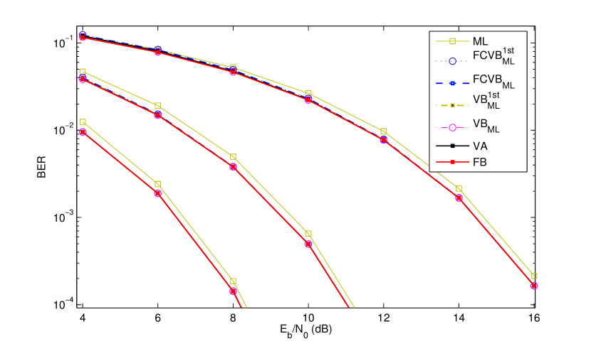
Figure 8.1.1: BER versus SNR per bit, $E_{b}/N_{0}$ (dB), for $2,8,64$-QAM (left,middle,right), with $10^{5}$ Monte Carlo runs.

In Fig. 8.1.1, the BER performance is plotted versus $E_{b}/N_{0}$, for the competing schemes in Chapter 6. In all cases of $M\in\{2,8,64\}$, ML is the worst estimator, as anticipated in Section 6.7.1, while the performances of all other algorithms are identical. Intuitively, this is an expected result for VB approximation and its variant, FCVB, all of which seek an approximating distribution in the class $\mathcal{F}_{c}$ and $\mathcal{F}_{\delta}$, respectively, of independent distributions. The reason is that the correlation coefficient, $\rho$, implied by a transition matrix with uniform elements, is low.

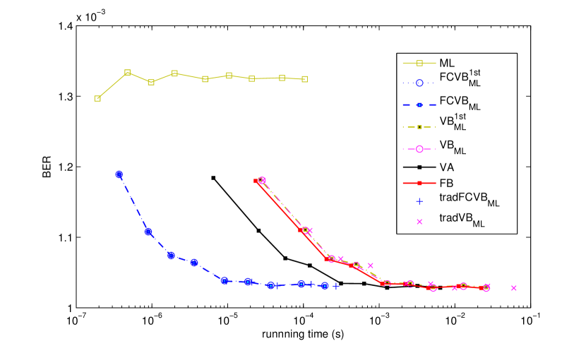
Figure 8.1.2: BER versus running-time for 64-QAM, with $10^{5}$ Monte Carlo runs. From left to right: $n=\{2,5,10,20,50,100,200,500,1000\}$. The running-time is measured by C++ implementation and 3 GHz Core2Duo Intel processor.

The effect on performance of a constrained running-time is illustrated in Fig. 8.1.2, in which we set $M=64$ , $E_{b}/N_{0}=14.5$ (dB), and we varied the number of data $n$ such that BER performance of all methods are convergent to $10^{-3}$. In this scenario of high SNR, the algorithms have almost identical performance, but with different running-times. Hence, all curves in Fig. 8.1.2 appear as x-shifted variants of each other.

The results show that, given a fixed-time resource, we can run the low complexity FCVB with more data than is possible for other algorithms. The maximum gain in FCVB’s performance over VA’s is about $12$%, with a fixed time resource around $10$ microseconds. The simulation results in Fig. 8.1.2, for the case $n=50$, are also extracted in Fig. 8.1.3 in order to illustrate the superiority of the Accelerated $FCVB_{(ML)}$ to VA and FB methods.

As explained in Section 6.7.1, the FB algorithm is the most accurate method, since it returns the sequence of marginal MAP estimates of the HMC labels, i.e. the exact minimum risk (MR) estimate in this case (4.3.8). The VA and $FCVB_{(ML)}$, despite of not being MR risk estimators, return the exact global and local MAP trajectory estimate for the HMC, respectively. For the weakly correlated HMC model in Fig. 8.1.3, we can see that these two methods are very close, to the extent that they are visually identical to FB in performance.

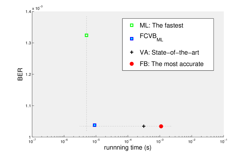
Figure 8.1.3: BER versus running-time for 64-QAM (extracted from Fig. 8.1.2, with the case $n=50$).

8.1.3 Computational load of HMC source estimates

For brevity, we only consider the accelerated scheme for VB-based inference here. The comparison between traditional and accelerated schemes will be studied in Section 8.1.4.

From Table 6.6.1, we can roughly estimate the cost of each algorithm via the number of equivalent operators. by normalizing the cost of $ML$ as $O(1)$, as follows (from the lowest to highest anticipated cost):

• For FCVB: By normalizing the cost of $ML$ as $O(1)$, the cost of each FCVB cycle and VA should be $O(1)$ and $O(M)$, respectively. Because $FCVB_{(ML)}$ requires at least one IVB cycle $O(\eta\nu_{e})$ and $O(1)$ $ML$-based initialization, in respect to ML’s cost, the total cost of $FCVB_{(ML)}$ should be at least $O(\eta\nu_{e}+1)\geq O(1.75)$, where $\nu_{e}\geq 1$ and $\eta\in\left[0.75,1.25\right]$, as explained in Section 6.6.2.2.

• For VA: the cost should be $O(M)$.

• For FB: because the cost of MUL is not deterministic, we consider FB to be at least three times slower than VA, as is often noted in the literature [Wu (2000)].

• For VB: Each VB cycle is slightly slower than FB, hence the total cost of $VB_{(ML)}$ is at least $\nu_{e}$-fold slower than FB.

In summary, we can predict the running time of $FCVB_{(ML)}$, $VA$, $FB$ and $VB_{(ML)}$ versus $ML$’s to be $O(\eta\nu_{e}+1)\geq O(1.75)$, $O(M)$, $O(3M)$ and $O(3M\nu_{e})$, respectively.

Let us verify above computational prediction via the simulation results in Fig. 8.1.2, $M=64$. the average ratios of running time of $FCVB_{(ML)}$, $VA$, $FB$ and $VB_{(ML)}$ versus $ML$’s were found to be $1.83$, $57.1$, $200.3$ and $233.9$, respectively. These results are consistent with our estimates of the ratios in the last paragraph.

Also, from Fig. 8.1.2, we can see that FCVB is completely superior to VA in this case, since they achieve similar performance, given the same number $n$ of data, but FCVB runs much faster. The average gain in FCVB’s speed over VA’s is about $57.1/1.83=31.2$ times, i.e. around half of $M=64$. This gain in simulation is also consitent with the theoretical gain $M/(\eta\nu_{e}+1)\leq 36.6$ in computational load, with $M=64$, $\nu_{e}\geq 1$ and $\eta\in\left[0.75,1.25\right]$, as explained above.

In the same simulation of Fig. 8.1.2, we also found that the average $\bar{\nu_{e}}$ for $FCVB_{(ML)}$ is $\bar{\nu_{e}}=1.01$, i.e. $FCVB_{(ML)}$ almost converged right after the first IVB cycle. Then, we can deduct the average value $\bar{\eta}$ to be $\bar{\eta}=\frac{(1.83-1)}{\bar{\nu_{e}}}=0.82$. This value $\bar{\eta}=0.82$ belongs to the theoretical range $\left[0.75,1.25\right]$.

Remark 8.1.1.

Note that, if we exclude the relative cost $O(1)$ of ML’s initialization step in the $FCVB_{(ML)}$’s relative cost $O(\eta\nu_{e}+1)$, the average computational load $\overline{\eta\nu_{e}}$ of Accelerated FCVB algorithm in this case is only $\overline{\eta\nu_{e}}=1.83-1=0.83$ times of $ML$’s cost, i.e., in this case, the Accelerated FCVB is faster than the currently-supposed fastest algorithm, ML, for HMC estimate.

8.1.4 Evaluation of VB-based acceleration rate

From two Lemmas 6.5.1-6.5.2, the BER performance for accelerated scheme is expected to be the same as traditional scheme for VB-based (VB and FCVB) inference, which is indeed the case in simulations in this chapter. For comparison purpose, the gain factor in this case is the acceleration rate $\frac{\nu_{c}}{\nu_{e}}$ in speed, as defined in (6.5.15), between the effective number $\nu_{e}$ and total number $\nu_{c}$ of IVB cycles.

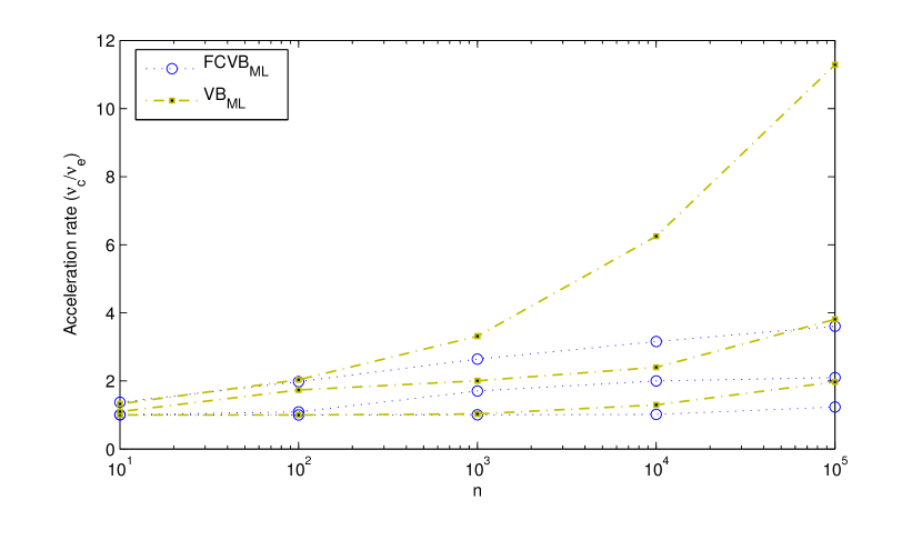
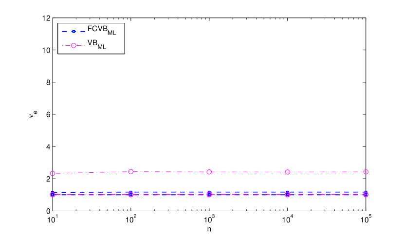
Figure 8.1.4: Acceleration rate $\nu_{c}/\nu_{e}$ (above) and effective number $\nu_{e}$ of IVB cycles (below) versus number of data $n$, with $10^{3}$ Monte Carlo runs.. Three curves for each algorithm, from bottom to top, correspond to number of states: $M=\{2,8,64\}$. Note that, some curves are almost identical to each other.

In Fig. 8.1.1, the overall average values of $\nu_{c}$ for $tradVB_{(ML)}$ and $tradFCVB_{(ML)}$ and those of $\nu_{e}$ for $VB_{(ML)}$, $FCVB_{(ML)}$ are $2.6\pm 0.7$, $1.5\pm 0.3$ and $1.6\pm 0.6$, $1.1\pm 0.1$ over $10^{5}$ Monte Carlo runs, respectively. Hence the acceleration rate $\nu_{c}/\nu_{e}$ in this context is about $1.5$ for these VB and FCVB schemes.

In Fig. 8.1.4-8.1.5 (lower panels), we can see that $\nu_{e}$ for both $VB_{(ML)}$ and $FCVB_{(ML)}$ are very small, $O(1)$, and independent of $n$, even at $n=10^{5}$. At high values of $M$ ($32$ and $64$), $\nu_{e}$ for $VB_{(ML)}$ increases considerably, while $\nu_{e}$ for $FCVB_{(ML)}$ increases only slightly.

Compared with $tradVB_{(ML)}$ and $tradFCVB_{(ML)}$, we can see that the acceleration rate of $FCVB_{(ML)}$ is approximately linear in the $\log$ of $n$ or $M$, i.e. $O\left(\frac{\nu_{c}}{\nu_{e}}\right)=O(\log M)$ and $O\left(\frac{\nu_{c}}{\nu_{e}}\right)=O(\log n)$, with fixed $n$ and fixed $M$, respectively. The acceleration rate of $VB_{(ML)}$ is super-linear against a $\log$ scale, when $n$ and $M$ are high. Hence, for $VB_{(ML)}$, we have $O\left(\frac{\nu_{c}}{\nu_{e}}\right)\geq O(\log M)$ and $O\left(\frac{\nu_{c}}{\nu_{e}}\right)\geq O(\log n)$, with fixed $n$ and fixed $M$, respectively. As a consequence, from simulation results of $\nu_{e}$ and acceleration rate $\frac{\nu_{c}}{\nu_{e}}$, we can deduct that the converged IVB cycles, $\nu_{c}$, of $tradVB_{(ML)}$ and $tradFCVB_{(ML)}$ are also logarithmically scale against both $n$ and $M$.

Overall, this $\log$scale phenomenon may be relevant to exponential forgetting property of HMC, as explained in Section 6.7.2. The simulations also show that VB requires slightly more number of IVB cycles than FCVB, possibly because FCVB circulates hard-information, which is likely to converge faster than soft-information used in VB.

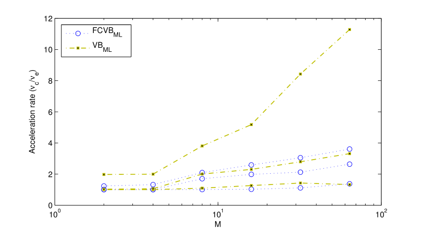
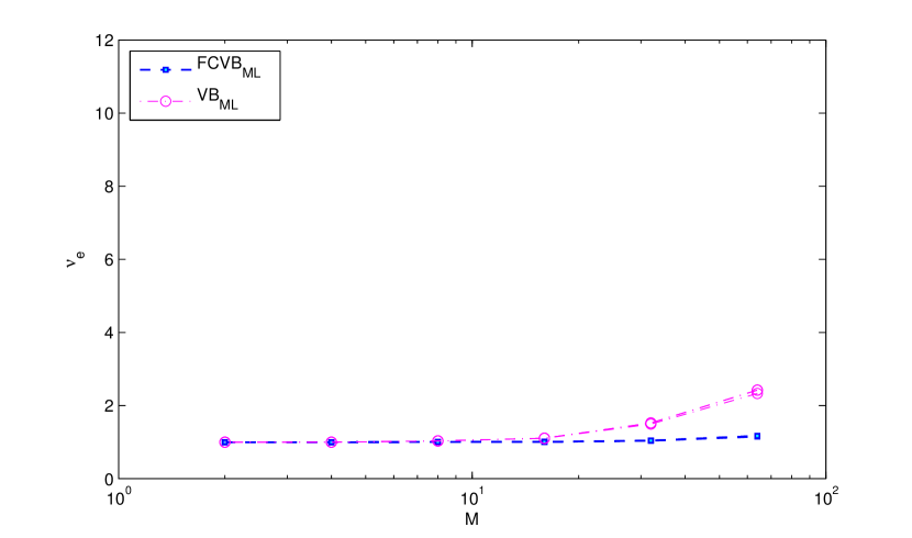
Figure 8.1.5: Acceleration rate $\nu_{c}/\nu_{e}$ (above) and effective number $\nu_{e}$ of IVB cycles (below) versus number of states $M$, with $10^{3}$ Monte Carlo runs.. Three curves for each algorithm, from bottom to top, correspond to number of data: $n=\{10^{1},10^{3},10^{5}\}$. Note that, some curves are almost identical to each other.

8.2 Rayleigh fading channel

Although the Rayleigh fading channel was thoroughly reviewed in Section 3.3, some key points for simulation will be summarized here for clarity.

Let us recall that, in practice, the receiver may be moving with velocity $v$. Because of the Doppler effect, this movement causes a fading rate $g_{i}\triangleq\left\|h_{i}\right\|$ (3.3.4) for the amplitude’s average of scattering received signals, as illustrated in Fig. 3.3.1. A statistical model for $|h_{i}|$, firstly proposed in [Clarke (1968)], is an envelope of a stationary complex Gaussian process, whose autocorrelation function (ACF) is given by (3.3.7):

$$\rho(T_{s})=\sigma^{2}J_{0}(2\pi f_{D}T_{s})$$ (8.2.1)

where $\sigma^{2}$ is the variance of the complex Gaussian process per dimension, $f_{D}=v/\lambda$ (Hz) is the maximum Doppler frequency, $\lambda$ (m) is the transmitted carrier wavelength, $J_{0}(\cdot)$ is the zero-order Bessel function of the first kind and $T_{s}$ is the sampling period. Note that, at any sampling time $i=\{1,\ldots,n\}$, the marginal distributions of $\bar{g}_{i}$ and $\bar{g}_{i}^{2}$ for this Gaussian process are Rayleigh [Tan and Beaulieu (2000); Wang and Chang (1996)] and $\chi^{2}(2)$ [Cavers (2000)] distribution, respectively, as shown in equations (3.3.10-3.3.11). Hence, this model is called a Rayleigh fading channel. Because it is prohibitive to evaluate $\bar{g}_{i}$ via ARMA process, a quantized HMC model [Sadeghi et al. (2008)] for $\bar{g}_{i}$ is currently a popular choice for the decoder over fading channel. In our simulation, all values of $\bar{g}_{i}$ are generated from the quantized HMC, as defined below.

8.2.1 Markov source with HMC fading channel

From receiver’s model in equation (3.3.5), let us consider a fading channel model, with the same Markov source $s_{i}$ and notations in previous section:

$$x_{i}=\bar{g}_{i}s_{i}+e_{i},\ i=\{1,\ldots,n\}$$ (8.2.2)

where $\bar{g}_{i}$ is one of quantized $K$-levels of Rayleigh distribution $f(g_{i})$. The transition matrix, $\mathbf{T}_{c}$, of fading HMC is a quantized version of the conditional distribution: $f(g_{i}|g_{i-1})=f(g_{i},g_{i-1})/f(g_{i})$, where $f(g_{i},g_{i-1})$ is a time-invariant bi-variate Rayleigh distribution (see Appendix. B for details). Then, the model (8.2.2) can be augmented to be an HMC with $MK$ states. Let us then define $MK\times MK$ transition matrix as $\mathbf{T}_{cs}=\mathbf{T}_{c}\bigotimes\mathbf{T}_{s}$, where $\bigotimes$ denotes Kronecker product for matrix. Because $K=8$ channel quantization levels are found to be accurate enough for $f_{D}T_{s}\leq 0.01$ [Sadeghi and Rapajic (2005)]. Then, in the sequel, let us consider an $M=16$-QAM signal transmitted over a Rayleigh channel, which yields an augmented source-channel HMC of $MK=128$ states. The algorithms for HMC in Chapter 6 will infer the $MK$-state label of the augmented HMC, $\bar{g}_{i}s_{i}$, in (8.2.2). We can then marginalize out the $K$ channel levels to compute the $M$-state Markovian source. Hence, the BER in our simulations took only the source state estimates into account.

For parameter settings, since $g_{i}$ and $s_{i}$ are assumed independent, the fading power $E(g_{i}^{2})=2\sigma^{2}$ is normalized to unity in this section, i.e. $\sigma^{2}=0.5$, so that the average SNR per bit $SNR_{b}$ is still the same as average energy per bit of the source, i.e. $SNR_{b}=E_{b}/N_{0}$ (Section 8.1). Also, as shown in (8.2.1), the correlation coefficient, $\rho\triangleq\rho(T_{s})$, of the time-invariant $f(g_{i},g_{i-1})$ is a function of the normalized Doppler frequency $f_{D}T_{s}$, whose meaning is explained in Section 2.3.5.3. This relationship is illustrated in in Fig. 8.2.1. Then, we can vary $\rho$ via three practical regimes of fading channel, i.e. slow, intermediate and fast fading regimes, corresponding to $f_{D}T_{s}\lesssim 0.01$, $0.01\lesssim f_{D}T_{s}\lesssim 0.4$, and $f_{D}T_{s}\gtrsim 0.4$, respectively [Sadeghi et al. (2008)]. Because the exact thresholds for those three regimes are not clearly defined in the literature, let us re-define the range $f_{D}T_{s}\leq 0.01$, $0.01<f_{D}T_{s}\leq 0.1$, and $f_{D}T_{s}>0.1$ for those three regimes, respectively, in this thesis.

Note that, the correlation in $\mathbf{T}_{c}$ is implied by value of $\rho$ in (8.2.1). Because the correlation in our uniform samples-based $\mathbf{T}_{s}$ is low, the correlation in $\mathbf{T}_{cs}$ mostly depends on $\rho$. Hence, by varying $\rho$, we are actually varying the correlation in the augmented HMC model (8.2.2).

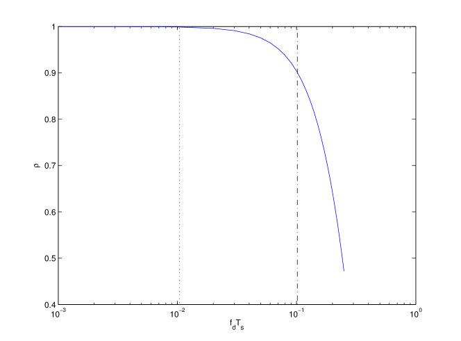
Figure 8.2.1: Correlation coefficient $\rho=J_{0}(2\pi f_{D}T_{s})$ versus normalized Doppler frequency $f_{D}T_{s}$. From left to right: three fading regimes are slow, intermediate, and fast fading regimes, corresponding to $f_{D}T_{s}\leq 0.01$, $0.01<f_{D}T_{s}\leq 0.1$, and $f_{D}T_{s}>0.1$, respectively.

8.2.2 Performance of source estimates in HMC channel

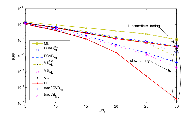
Figure 8.2.2: BER versus SNR per bit, $E_{b}/N_{0}$(dB), for HMC source ($M=16$-QAM)) over HMC fading channel ($K=8$ levels), with $10^{5}$ Monte Carlo runs.

For evaluating performance, the simulation against variable SNR per bit, $E_{b}/N_{0}$, is displayed in Fig. 8.2.2. Two values $f_{D}T_{s}=0.01$ and $f_{D}T_{s}=0.1$ are considered as slow and intermediate fading regimes, respectively, in this figure.

We can see that, in the fast fading regime, the correlation coefficient $\rho$ is not too high (less than $0.9$), all the algorithms (except ML) have the same performance and similar to those for the toy HMC example in Fig. 8.1.1. This result is expected, because when the fast fading channel becomes dominant, the samples between two time point becomes more independent. In the slow fading regime, which is more popular in practice [Sadeghi and Rapajic (2005)], the performances of both FB and VA are almost coincide with each other and better than those in the fast fading regime. However, VB’s and FCVB’s performance become closer to ML than to FB or VA in high SNR per bit. This fact implies that VB and FCVB approximations become less and less accurate. In order to corroborate this finding, two plots of BER and $KLD_{\widetilde{f}||f}$ versus $\rho$ are displayed in Fig. 8.2.3 and Fig. 8.2.4, respectively (for the computation of $KLD_{\widetilde{f}||f}$, see Section 6.6.1.2).

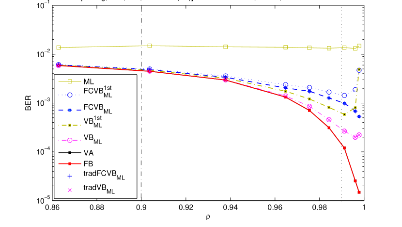
Figure 8.2.3: BER versus correlation coefficient $\rho$ of Rayleigh channel, at $E_{b}/N_{0}=30$ dB, for three fading regimes in Fig. 8.2.1, with $10^{5}$ Monte Carlo runs.

In Fig. 8.2.3, we focus on the case $E_{b}/N_{0}=30$ dB in Fig. 8.2.2. By varying the fading channel from slow to fast regimes, i.e. from $f_{D}T_{s}\leq 0.01$ up to $f_{D}T_{s}\geq 0.1$, we can investigate many cases, $\rho\geq 0.99$ down to $\rho\leq 0.9$, respectively. In all cases, ML’s performance does not change and remains with the worst performance. For the fast regime ($\rho\leq 0.9$), all algorithms (except ML) have virtually the same performance. For the intermediate regime, $0.9\leq\rho\leq 0.99$, there is a trade-off in performance between two groups of exact and approximate estimates, i.e. between FB (and VA) and VB (and FCVB). For the slow regime ($\rho\geq 0.99$), although VB and FCVB’s estimates are still better than ML’s, their performance deteriorates compared to FB and VA.

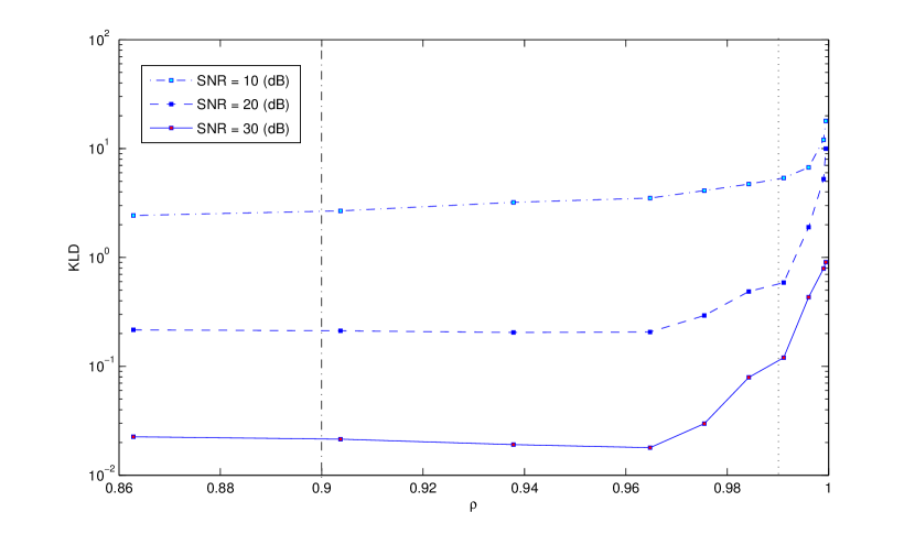
Figure 8.2.4: $KLD_{\widetilde{f}||f}$, for the VB approximation of source-channel HMC, versus $\rho$, for the slow fading regime in Fig. 8.2.2, with $10^{4}$ Monte Carlo runs.

The dependence of VB’s accuracy of approximation on $\rho$ is shown clearly in Fig. 8.2.4. For fast and intermediate regimes ($\rho\leq 0.99$), $KLD_{\widetilde{f}||f}$ is small, implying that VB yields a good approximation. For the slow regime ($\rho\geq 0.99$), the $KLD_{\widetilde{f}||f}$ increases sharply with $\rho$, and, hence, VB for the HMC is not a good approximation under this fading conditions. Since FCVB is a CE-based version of VB, the trend of $KLD_{\widetilde{f}||f}$ in Fig. 8.2.4 explains the diminished performance of VB and FCVB compared to FB and VA, observed in Fig. 8.2.3. We also see that this phenomenon is repeated for many values of SNR per bit $E_{b}/N_{0}$, although $KLD_{\widetilde{f}||f}$ becomes smaller (i.e. VB yields a better approximation) in higher SNR regimes, as expected.

The empirical results on relationship between digital detection accuracy and correlation coefficient $\rho$ also proposes a trade-off situation in practice:

• By increasing $\rho$, the performance of Markov-based algorithms (i.e. FB and VA), is likely to be increased, but the approximations in class of independent distributions (i.e. VB and FCVB) is decreased. The higher $\rho$ is, the more significant this phenomenon becomes. This fact is actually reasonable, since the original model become more correlated in this case.

• In simulations, it is shown that there are three working regimes for FCVB algorithm. If correlation in transition matrix of HMC is not high ($\rho\leq 0.9$), FCVB can achieve the same performance as VA and FB. When the correlation is high ($0.9\leq\rho\leq 0.99$), FCVB yields a trade-off between performance and computational load. And finally, if the correlation is too high ($\rho\geq 0.99$), FCVB is not an attractive algorithm, since approximations in independent class for HMC are not suitable.

8.2.3 Computational load of source estimates in HMC channel

The average running time (over all tested $\rho$) of all algorithms in Fig. 8.2.3 are displayed in Fig. 8.2.5. This result shows that FCVB is an attractive algorithm, with much lower complexity than VA. The ratios of averaged running-time of $FCVB_{(ML)}$, $VA$, $FB$ and $VB_{(ML)}$ versus $ML$’s are $2.03$, $139.7$, $399.7$ and $575.4$, respectively. For the number of IVB cycles, we have $\nu_{e}=1.04\pm 0.04$, $\nu_{c}=1.79\pm 0.54$ and $\nu_{e}=1.24\pm 0.10$, $\nu_{c}=2.28\pm 0.64$ for $FCVB_{(ML)}$, $tradFCVB_{(ML)}$ and $VB_{(ML)}$, $tradVB_{(ML)}$, respectively. Hence, the acceleration rate is about $1.25$ for both FCVB and VB schemes in this augmented HMC context. These results are all consistent with Table 6.6.1, and with the explanation in sections 8.1.3-8.1.4.

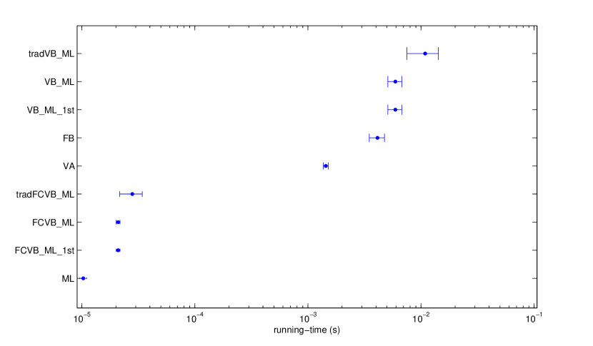
Figure 8.2.5: Running-time averaged over all tested $\rho$ in Fig. 8.2.3, with $10^{5}$ Monte Carlo runs. The running-time is measured by C++ implementation and 3 GHz Core2Duo Intel processor.

8.3 Summary

This chapter presents simulation results in the context of two digital receiver models, developed in Chapter 3. The first assumes a Markov source, whose transition matrix was generated uniformly and simulated as input to a synchronized AWGN channel. In the simulations, the accuracy of all state-of-the-art algorithms FB, VA and ICM (i.e. FCVB) was shown to be the same, but the accelerated ICM/FCVB algorithm reduced the effective number of iteration cycles to about one, on average.

Secondly, the same Markov source was used as an input to a synchronized finite state Markov fading channel, with number of data, $n$, and number of states, $M$. In this case, although the computational load $O(nM)$ of the accelerated FCVB scheme was still much smaller than $O(nM^{2})$ of VA, its accuracy was only comparable to VA’s when the correlation coefficient of Rayleigh fading process was not too high. This trade-off facility can be applied in other contexts, as discussed in the next chapter.

Chapter 9 Contributions of the thesis and future work

The pathway established in Chapter 2 has ended. It started by reviewing the telecommunications literature for the purpose of identifying the main challenges that we wanted to address using Bayesian methodology. The interior chapters have provided progress with this aim. In this closing chapter, we will summarize the contributions of the thesis and offer suggestions for future work, before closing the thesis with concluding remarks.

9.1 Progress achieved by the thesis

In this section, the strengths and weaknesses of the thesis will be reflected by considering the major contributions and suggesting future work. In turn, these can be divided into four principal themes, corresponding to four key tasks in Chapter 1. For each theme, the discussion will be presented in three steps: key achievements in this thesis, the generalization, and proposals for future work.

9.1.1 Optimizing computational flow via ring theory

For this theme, the thesis’ purpose is to reduce the computational load involving the evaluation of objective functions arising in inference problems relevant to telecommunication.

• Main contributions:

The thesis’ original idea is to separate computational flow into two domains: operators and variables (Section 5.2). Respectively, two key contributions are: in the former domain, a novel theorem (Theorem 5.3.7) on the computational perspective of the generalized distributive law (GDL) in ring theory, and in the latter domain, no-longer-needed (NLN) algorithm (Algorithm 5.1). The theorem guarantees computational reduction for any valid application of GDL upon operators, while the NLN algorithm exploits the conditionally independent (CI) topology of variables. Together, they open up two other contributions. The first one is the efficient Forward-Backward (FB) computational flow (Section 5.4) for distributing the operators over variables when needed, while the second one is the discovery of explicit formulae for counting the number of operators, ring-sum and ring-products (Section 5.3.3), in that FB flow.

In general probability context, there is an increase exponentially of number of operators with the number of data in computation of the joint distribution, because the number of state increases exponentially (the curse of dimensionality). However, the number of operators falls exponentially with the number of NLN variables. In hidden Markov chain context, the FB algorithm and VA, two special cases of FB recursion, exploit the latter in combating the former. Hence, the FB recursion and GDL helps interpret the linear dependence on data in the complexity of FB and VA, as a consequence of numerical cancellation over the number of operators.

• Generalization:

In principle, the recursive FB flow is applicable to objective functions to which GDL is valid. For example, it is applicable to computation of the message-passing algorithm in graphical learning [Aji and McEliece (2000); Moon (2005)] and Markov random field [Geman and Geman (1984)], computation of marginalization, maximization, entropy in Bayesian learning, evaluation of Iterative VB algorithm [Smidl and Quinn (2006); Wainwright and Jordan (2008)].

• Future work:

Based on the above generalization, future work can be designed in two directions: optimizing the FB flow and finding more applications.

- For the former: the objective is to find the CI topology that minimizes the computational reduction achieved via FB recursion. Although the global minimization is an NP-complete problem, as discussed in Section 5.4.3, a local solution can be found by extending the computational flow from two-directions in FB recursion to multi-directions in a topological graph. Another potential solution is to apply topological sorting algorithms to the CI topology before implementing the FB recursion, owing to the explicit formulae for determining computational complexity in this case.

- For the latter: the objective is to verify whether GDL is valid for a particular objective function. One key property is Markovianity, owing to its natural CI topology. Because Markovianity is assumed in many efficient algorithms in telecommunications system, as reviewed in Section 2.3, the FB recursion can be applied to studying the computational reduction in these algorithms, e.g. in forward-backward lattice filters and in other scenarios in telecommunications. Another interesting issue is to explore the relationship between recursion (Section 6.4) and iteration (Section 6.6) in Markovian objective functions. If the recursion is carried out via GDL, it is likely that the computational load can be further reduced in two cases: recursion embedded in iteration, and iteration embedded in recursion. The first case was considered in Accelerated FCVB algorithm in this thesis (Section 6.6.2), while the second case can be explored in future online variance of VB scheme.

9.1.2 Variational Bayes (VB) inference

For this theme, the thesis’ purpose is to extend the VB methodology in order to achieve more accurate deterministic distributional approximation. Our aim was not to reduce computational load, per se.

• Main contributions

The thesis’ original idea is to weaken the coupling between parameters in the transformed metric by diagonalizing the Hessian matrix at a specific point. The VB approximation is then applied to the transformed posterior distribution. The technique is referred to as the transformed VB (TVB) approximation (Section 7.2). Compared with VB, the TVB scheme was shown to yield significant improvement in accuracy when the Hessian of the transformed distribution is designed to be diagonal at its MAP point. Intuitively, this improvement is achieved because the transformed variables are asymptotically independent, in which case the VB approximation is exact. Note that, the TVB approximation has a fundamental output as an approximate distribution in the original metric (Fig. 7.1.1), a novel contribution, when compared to classical orthogonalization approaches, whose purpose is to produce estimates of transformed variables.

• Generalization:

In principle, the TVB approximation is applicable to any multivariate posterior distribution, whose desired marginalization is intractable. In practice, for tractability of Iterative VB algorithm, the transformed distribution should be separable-in-parameters (Definition 4.5.2), i.e its logarithm can be factorized into product of functions for each parameter separately.

• Future work:

Based on the above generalization, future work can be designed in two directions: optimizing computational load and designing new transformations, such that the transformed distribution is separable-in-parameter (Definition 4.5.2).

- For the former: the current TVB approximation may involve computational intensive IVB cycles. A potential solution is to replace the involved expectation with maximization via the FCVB scheme (Lemma 4.5.3). However, this scheme reduces to a point estimation and neglects all the moments, which, in turn, may significantly reduce the quality of distributional approximation (Fig. 8.2.3).

- For the latter: Two potential transformations are global diagonalization of transformed Hessian matrix and frequentist’s transformation techniques [Box and Cox (1964); Sakia (1992); Koekemoer and Swanepoel (2008)]. The task is, however, not trivial, because of difficulty with each of transformation design. Global diagonalization of the Hessian matrix is only feasible for bivariate distribution [Cox and Reid (1987)]. Furthermore, in frequentist’s transformation, the inverse transformation can be applied in the point estimate. In contrast, the inverted distribution, i.e. the TVB approximation, may be highly complicated and, in particular, its marginalization is not available.

These difficulties show that further work are required for TVB. Even in the current form, TVB needs to be applied on a case-by-case basis, since the certainty equivalent (CE) points, like the MAP point, may not be available at the beginning. Nevertheless, the TVB shows the potential for relaxing VB methodology to achieve more accurate distributional approximation.

9.1.3 Inference for the Hidden Markov Chain

The previous two themes focus exclusively on computational reduction and enhancing accuracy, respectively, but not on both together. The third main theme of this thesis is to provide new algorithms which achieves better trade-offs between performance and speed for label’s inference in the HMC.

• Main contributions:

The thesis’ idea is to replace the VA with the ICM algorithm for better trade-off. Two contributions, one for performance and one for speed, were achieved using this approach.

- For performance, a Bayesian interpretation was given for both the ICM (Section 4.5.2.4) and the VA algorithm (Section 6.4.3). We show that the criteria are to preserve the global MAP trajectory and the local MAP trajectory at any recursive and iterative step, respectively. This interpretation also explained why the accuracy of VA and ICM are comparable when correlation in the HMC is not too high.

- For speed, an accelerated scheme was designed for the VB scheme, in which any VB marginals that have converged are flagged and are not updated in the next IVB iteration. We shows that this accelerate scheme provides the same output as original scheme (Lemma 6.5.1,6.5.2). Since ICM can be re-interpreted as the functionally constrained VB (FCVB) approximation, the computational load of Accelerated ICM/FCVB was reduced, in simulation, from $O(\nu nM)$ down to nearly $O(nM)$, where $\nu$, $n$ and $M$ are number of ICM iterations, number of time points and number of states in HMC, respectively.

• Generalization:

In principle, the accelerated scheme for Iterative VB and ICM algorithm can be applied to any inference problem involving hidden field of CI variables, notably the Markov random field, when correlation is not too strong.

• Future work:

Based on the above principle, we may investigate further the computational reduction achieved by the accelerated scheme. The simulation in the thesis showed that, in the HMC, the number of iteration for traditional VB and ICM/FCVB is almost linear to the logarithm of both $n$ and $M$ (Section 8.1.4). Also, the effective number of IVB cycle for accelerated VB and ICM/FCVB scheme was close to one and stayed nearly constant with $n$ and $M$ (Section 8.1.4). This reduction in log-scale suggests HMC’s exponentially-forgetting property, whose influence on the number of IVB cycle should be investigated.

9.1.4 Inference in digital receivers

For this theme, the thesis’ purpose is to apply the three themes above to practical concern in the digital demodulation in digital receivers.

• Main contributions:

The thesis’ idea was to apply the Accelerated ICM/FCVB algorithm and TVB approximation to demodulation in digital receivers. Two main contributions, one for Markovian digital detector and one for frequency synchronization, were given in the thesis.

For Markovian digital detector (Chapter 8), the Accelerated ICM/FCVB algorithm was applied to detecting modulated bit stream transmitted over a quantized Rayleigh fading channel. When the fading is not too slow, i.e. correlation between samples is not too high, the performance of Accelerated ICM/FCVB is comparable to the state-of-the-art VA, but with a greatly reduction of computational load (Section 8.1.3,8.2.3).

For frequency synchronization, the full Bayesian inference was studied for a toy problem, namely frequency inference for the single-tone sinusoidal model in AWGN channel (Section 7.4). Note that, when the frequency is off-bin, the posterior mean yields far more accurate (Fig. 7.4.1) than periodogram-based ML estimate, since posterior mean is continuous value while the DFT-based periodogram is not (Section 7.4.4.1). The accuracy of the TVB approximation was also found significantly better than that of the VB approximation (Fig. 7.4.1) from the point of view of posterior mean (Remark 7.4.1). It is important to remember that all of these techniques - VB, TVB, and exact posterior mean, as well as ML - are all computed via the DFT (and implemented via FFT), and therefore have similar computational load.

• Generalization:

In principle, the Accelerated ICM/FCVB can be successfully applied to the finite-state Markov channel (FSMC) [Sadeghi et al. (2008)] when correlation is not too high. Also, the TVB method is attractive for maintaining accuracy in nonlinear synchronization problem [Quinn et al. (2011)].

• Future work:

Based on the above principle, future work can be proposed in two directions: Markovian digital decoder and carrier synchronization.

- For Markovian digital decoder (Chapter 8), perhaps the most obvious proposal is to replace the VA with the Accelerated ICM/FCVB. The evidence supporting proposal was provided in (Fig. 8.1.2,8.1.3,8.2.5), showing great increase in speed without much loss of accuracy. Note that, the Accelerated ICM/FCVB is more broadly applicable than the Markovian context of VA. Furthermore, the Accelerated ICM/FCVB can be implemented in both online and offline scenarios, yield the same output in these cases, while VA is the offline algorithm.

- For carrier synchronization, the Bayesian inference is mostly preferred when the accuracy is a premium. For example, the accuracy in frequency and phase synchronization is critical in OFDM scheme for 4G system (Section 2.3.4.1), and in joint decoding and synchronization [Herzet et al. (2007)]. In the future, the challenge will to elaborate VB and TVB solution for these problems.

9.2 Conclusion

The thesis has considered both the computational side of VB-based inference methodology and its application in digital receivers.

For the inference tasks we considered, the mathematical tools were Bayesian methodology and ring theory, whose purpose is to update the belief on unknown quantities and to generalize the operators for computing these beliefs, respectively. The required computations were efficiently implemented via two approaches, namely recursive flow via the generalized distributive law (GDL) from ring theory, and iterative deterministic approximation via the Variational Bayes (VB) approximation in mean field theory. Two key contributions were given for each of the two approaches. For GDL, the first contribution was a novel theorem on GDL, guaranteeing the reduction in the number of operators and providing the formula for quantifying this reduction. Secondly, a novel Forward-Backward (FB) recursion for achieving this reduction was derived. Meanwhile, for VB, the first contribution was the Transformed VB (TVB) scheme for asymptotically decoupling the transformed distribution to which VB is applied. Secondly, we develop a novel accelerated scheme for VB, reducing the effective number of iterative VB cycles to about one in the case of hidden Markov chain (HMC) inference.

For digital receivers, the four achievements in inference methodology above were then applied to digital demodulation, which consists of synchronization and digital detection. Respectively, a TVB-based frequency synchronizer and a fast digital detector for the quantized Rayleigh fading channel were derived in the thesis. Each performs well in specific operating conditions, specified in Section 7.4 and Section 8.2, respectively. However, further work is needed to formalize these operating conditions and to achieve a robust extension of the algorithms. Nevertheless, these two applications illustrate the applicability to telecommunications systems of the novel inference methodologies, described in the previous paragraph. Undoubtedly, these approaches can address the technical demands of digital decoders in 4G mobile systems, as reviewed in Section 2.1.2.2.

As an outcome of this thesis, two related journal papers, based on Chapter 5 and Chapter 6 respectively, are about to be submitted to the IEEE Transactions on Information Theory. The novel algorithms derived from the generalized distributive law (GDL) in Chapter 5, which will be reported in the first of these papers, should have impact in the future design of optimal computational flows for arbitrary networks, particularly Bayesian networks. The novel Variational Bayes (VB) variants of the Viterbi algorithm, developed in Chapter 6 of this thesis, will be published in the second of these forthcoming journal papers, and were partly published in [Tran and Quinn (2011b)]. As explained in Chapter 6, these methods lead to better trade-offs between computational load and accuracy than the state-of-the-art Viterbi algorithm, and should yield more efficient decoders for hidden Markov chains. Note that preliminary work on Bayesian inference of hidden discrete fields was published in [Tran and Quinn (2010)]. Finally, Chapter 7 of this thesis, which proposes a novel inference scheme for frequency inference, was partly published in [Tran and Quinn (2011a)]. A fuller account of the TVB methodology in signal processing will be submitted to the IEEE Transactions on Signal Processing at the end of this year.

Appendix A Dual number

A dual number $d\in\mathbb{D}\subset\mathbb{R}^{2\times 2}$ [Yaglom (1968); Veldkamp (1975)] may be defined in two ways, as either (i) $d=a\mathbf{I}_{2}+b\boldsymbol{\epsilon}=\left[\begin{array}[]{cc}a&b\\ 0&a\end{array}\right]$, $a\in\mathbb{R}$ is called the real part and $b\in\mathbb{R}$ is called the dual part, or (ii) $d=\{Re(d),Im(d)\}$, i.e. :

$$Re(d) \triangleq a\mathbf{I}_{2}=a\left[\begin{array}[]{cc}1&0\\ 0&1\end{array}\right]$$

$$Im(d) \triangleq b\boldsymbol{\epsilon}=b\left[\begin{array}[]{cc}0&1\\ 0&0\end{array}\right]$$

where the latter is a Catersian form representation of $d$ alternatively, writing $d=a(\mathbf{I}_{2}+\frac{b}{a}\boldsymbol{\epsilon})$, and $\mathbf{I}_{2}\triangleq\left[\begin{array}[]{cc}1&0\\ 0&1\end{array}\right]$ , $\boldsymbol{\epsilon}\triangleq\left[\begin{array}[]{cc}0&1\\ 0&0\end{array}\right]$. We can propose a polar-form, representation of $d$, as follows:

$$d=a\angle\tan\theta$$

with the argument $\tan\theta\triangleq b/a$ and $a\neq 0$. Then, with the sum and product in $\mathbb{D}$ defined as usual matrix sum and product, it is easy to verify that:

$$d_{1}+d_{2} = (a_{1}+a_{2})+\epsilon(b_{1}+b_{2})$$

$$d_{1}d_{2} = (a_{1}a_{2})\angle(\tan\theta_{1}+\tan\theta_{2})$$

where $\epsilon$ is called the dual unit, and $\epsilon^{2}=0$, corresponding to the matrix form:

$$\boldsymbol{\epsilon}\boldsymbol{\epsilon}=\mathbf{0}\triangleq\left[\begin{array}[]{cc}0&0\\ 0&0\end{array}\right]$$

Appendix B Quantization for the fading channel

Our aim is to derive the probability mass function (pmf) induced by quantization of the amplitude paramater of the Rayleigh fading channel. In common with the literature [Tan and Beaulieu (2000); Kong and Shwedyk (1999); Sadeghi and Rapajic (2005)], we design the quantization thresholds such that each quantized state, $\overline{g}_{k,i}$ of $g_{i},$ is equi-probable.

At each time $i$, the first-order Rayleigh distribution is quantized to $K$-levels, as follows:

$$f(g_{i})=\begin{cases}\frac{g_{i}}{\sigma^{2}}\exp\left(-\frac{g_{i}^{2}}{2\sigma^{2}}\right)&,\ g_{i}\geq 0\\ 0&,\ \mbox{otherwise}\end{cases}$$ (B.0.1)

where $E(g_{i}^{2})=2\sigma^{2}$ is called the fading energy and $\sigma^{2}$ is called the variance of underlying complex Gaussian process per dimension [Sadeghi et al. (2008)] (see Section 3.3.2 for details). Note that, the fading energy $E(g_{i}^{2})=2\sigma^{2}$ can also be found via distribution $f(g_{i}^{2})$, which is the $\chi^{2}$ distribution with two degree of freedoms in this case [Cavers (2000)]:

$$f(g_{i}^{2})=\chi_{g_{i}^{2}}^{2}(2)=\frac{1}{2\sigma^{2}}\exp\left(-\frac{g_{i}^{2}}{2\sigma^{2}}\right)$$

whose the mean is $E(g_{i}^{2})=2\sigma^{2}$.

For quantization, an equiprobable partitioning approach similar to [Tan and Beaulieu (2000); Kong and Shwedyk (1999)] will be applied. Let us consider the continuous distribution function (c.d.f) of Rayleigh distribution (B.0.1), as follows:

$$F(g_{i})=\begin{cases}1-\exp\left(-\frac{g_{i}^{2}}{2\sigma^{2}}\right)&,\ g_{i}\geq 0\\ 0&,\ \mbox{otherwise}\end{cases}$$ (B.0.2)

Now we can find $K$ thresholds $\zeta_{1},\ldots,\zeta_{K}$ of $K$ equiprobable intervals, i.e. $F(\zeta_{k})-F(\zeta_{k-1})=\frac{1}{K}$, with $\zeta_{0}=0$, which yields:

$$F(\zeta_{k})=k/K,\ k=1,\ldots,K$$ (B.0.3)

From (B.0.2), these $\zeta_{k}$ can be expressed in closed form, as follows:

$$\zeta_{k}=\sqrt{-2\sigma^{2}\log(1-\frac{k}{K})},\ k=1,\ldots K-1$$

where, for truncation at $k=K$, we set $\zeta_{K}=5$, since $F(\zeta_{K}=5)\approx 1-10^{-11}$, if $E(g_{i}^{2})=2\sigma^{2}=1$. Then, the state of quantized fading channel are defined as the continuous mean $\overline{g}_{k,i}$ of each interval:

$$\overline{g}_{k,i}=K\int_{\zeta_{k-1}}^{\zeta_{k}}g_{i}f(g_{i})dg_{i},\ k=1,\ldots,K$$

which can be computed numerically [Kong and Shwedyk (1999)]. Under this $K$-state quantization procedure, we can define the bivariate (second-order) pmf of the $K^{2}$-state samples. The bivariate Rayleigh probability for a pair $g_{i}$, $g_{j}$ is also quantized into $K\times K$ intervals, as follows:

$$\Pr[\overline{g}_{m,i},\overline{g}_{k,j}]=\int_{g_{i}=\zeta_{m-1}}^{g_{i}=\zeta_{m}}\int_{g_{j}=\zeta_{k-1}}^{g_{j}=\zeta_{k}}f(g_{i},g_{j})dg_{i}dg_{j}$$ (B.0.4)

where the integral of the bivariate distribution, $f(g_{i},g_{j})$, can be computed numerically via the following form of bivariate Rayleigh distribution $f(g_{i},g_{j})$ [Sadeghi and Rapajic (2005)]:

$$f(g_{i},g_{j}) = \frac{g_{i}g_{j}}{\sigma^{4}(1-\rho^{2})}\exp\left(-\frac{(g_{i}^{2}+g_{j}^{2})}{2\sigma^{2}(1-\rho^{2})}\right)I_{0}\left(\frac{g_{i}g_{j}}{\sigma^{2}}\frac{\rho}{(1-\rho^{2})}\right)$$ (B.0.5)

in which $I_{0}$ denotes zero-order modified Bessel function of the first kind and $\rho$ is the correlation coefficient between $g_{i}$ and $g_{j}$. Note that, when $\rho$ is very close to $1$, then the argument of $I_{0}(\cdot)$ in (B.0.5) is large. For computation in that case, we can replace the above $I_{0}(\cdot)$ with its approximation $I_{0}(x)\approx\exp(x)/\sqrt{2\pi x}$, for large $x$ [Bowman (1958)].

From (B.0.1) and (B.0.4), the conditional pmf of the quantized Rayleigh fading amplitude can be defined as $f(l_{i}|l_{i-1})=Mu_{l_{i}}(\mathbf{T}_{K}l_{i-1})$, where $l_{i}\in\{\boldsymbol{\epsilon}(1),\ldots,\boldsymbol{\epsilon}(K)\}$ is label variable pointing to $K$ quantized levels $\overline{g}_{i}=[\overline{g}_{1,i},\ldots,\overline{g}_{K,i}]^{\prime}$ at time $i$ and $\mathbf{T}_{K}$ is positive $K\times K$ transition probability matrix of an homogeneous Markov chain, with elements: $t_{k,m}=\frac{\Pr[\overline{g}_{k,i},\overline{g}_{m,i-1}]}{\Pr[\overline{g}_{m,i-1}]}=\Pr[\overline{g}_{k,i},\overline{g}_{m,i-1}]\times K$, $1\leq k,m\leq K$. The columns of $\mathbf{T}_{K}$ are then normalized to 1, by definition, in order to avoid any numerical computation’s error. Finally, note that all initial probabilities of this Markov chain in this equi-probable scheme are equal to $1/K$, from (B.0.3).

References

- 3GPP (2005) 3GPP: 2005, ‘Technical specification group radio access network; Requirements for "Evolved UTRA (E-UTRA)" and "Evolved UTRAN (E-UTRAN)" (Release 7)’. Technical report, 3GPP TR 25.913.
- Ahmed (1991) Ahmed, N.: 1991, ‘How I came up with the discrete cosine transform’. Digital Signal Processing 1(1), 4–9.
- Ahmed et al. (1974) Ahmed, N., T. Natarajan, and K. R. Rao: 1974, ‘Discrete Cosine Transform’. IEEE Transactions on Computers C-23(1), 90–93.
- Aitchison and Dunsmore (1980) Aitchison, J. and I. R. Dunsmore: 1980, Statistical Prediction Analysis. CUP Archive.
- Aji and McEliece (2000) Aji, S. M. and R. J. McEliece: 2000, ‘The generalized distributive law’. IEEE Transactions on Information Theory 46(2), 325–343.
- Akaike (1974) Akaike, H.: 1974, ‘A new look at the statistical model identification’. IEEE Transactions on Automatic Control 19(6), 716–723.
- Aldrich (1997) Aldrich, J.: 1997, ‘R. A. Fisher and the Making of Maximum Likelihood 1912-1922’. Statistical Science 12(3), 162–176.
- Andersen (1970) Andersen, E. B.: 1970, ‘Sufficiency and Exponential Families for Discrete Sample Spaces’. Journal of the American Statistical Association 65(331), 1248–1255.
- Anderson and Svensson (2003) Anderson, J. B. and A. Svensson: 2003, Coded Modulation Systems. Springer.
- Arellano-Valle et al. (2006) Arellano-Valle, R. B., G. del Pino, and P. Iglesias: 2006, ‘Bayesian inference in spherical linear models: robustness and conjugate analysis’. J. Multivar. Anal. 97, 179–197.
- Armstrong (1933) Armstrong, E. H.: 1933, ‘Radio signaling system’.
- Arnold (2009) Arnold, B. C.: 2009, Advances in Mathematical and Statistical Modeling. Springer.
- Attias (1999) Attias, H.: 1999, ‘Inferring parameters and structure of latent variable models by Variational Bayes’. Electronic Proceedings of the Fifteenth Annual Conference on Uncertainty in Artificial Intelligence.
- Baddour and Beaulieu (2005) Baddour, K. and N. Beaulieu: 2005, ‘Autoregressive modeling for fading channel simulation’. IEEE Transactions on Wireless Communications 4(4), 1650–1662.
- Bahl et al. (1974) Bahl, L., J. Cocke, F. Jelinek, and J. Raviv: 1974, ‘Optimal decoding of linear codes for minimizing symbol error rate’. IEEE Trans. Inform. Theory 20, 284–287.
- Bard (1974) Bard, Y.: 1974, Nonlinear Parameter Estimation. Academic Press, New York.
- Bartlett (1948) Bartlett, M. S.: 1948, ‘Smoothing Periodograms from Time-Series with Continuous Spectra’. Nature (London) 161, 686–687.
- Baum et al. (1970) Baum, L. E., T. Petrie, G. Soules, and N. Weiss: 1970, ‘A Maximization Technique Occurring in the Statistical Analysis of Probabilistic Functions of Markov Chains’. The Annals of Mathematical Statistics 41(1), 164–171.
- Bayes (1763) Bayes, T.: 1763, ‘An Essay towards solving a Problem in the Doctrine of Chances’. Philosophical Transactions of the Royal Society of London 53, 370–418.
- Beal (2003) Beal, M.: 2003, ‘Variational Algorithms for Approximate Bayesian Inference’. Ph.D. thesis, University College London.
- Berger and Bernardo (1992) Berger, J. and J. Bernardo: 1992, ‘On the development of reference priors’. Bayesian Statistics 4, 35–60.
- Berger (1985) Berger, J. O.: 1985, Statistical Decision Theory and Bayesian Analysis. Springer.
- Bergmans (1995) Bergmans, J.: 1995, ‘Efficiency of data-aided timing recovery techniques’. IEEE Transactions on Information Theory 41(5), 1397–1408.
- Berlekamp (1968) Berlekamp, E. R.: 1968, Algebraic Coding Theory. New York: McGraw-Hill.
- Bernardo (1979) Bernardo, J.: 1979, ‘Reference posterior distributions for Bayesian inference (with discussion)’. J. Roy. Statist. Soc., Ser. B 41, 113Ð147.
- Bernardo and Smith (1994) Bernardo, J. M. and A. F. M. Smith: 1994, Bayesian Theory. John Wiley & Sons.
- Bernoulli (1713) Bernoulli, J.: 1713, Ars conjectandi, opus posthumum. Accedit Tractatus de seriebus infinitis, et epistola gallice scripta de ludo pilae reticularis. (English translation: The Art of Conjecturing, together with Letter to a Friend on Sets in Court Tennis (2005), Johns Hopkins Univ Press). Thurneysen Brothers.
- Berrou (2011) Berrou, C. (ed.): 2011, Codes and turbo codes. Springer.
- Berrou et al. (1993) Berrou, C., A. Glavieux, and P. Thitimajshima: 1993, ‘Near Shannon limit error-correcting coding and decoding’. pp. 1064–1070.
- Besag (1986) Besag, J.: 1986, ‘On the statistical analysis of dirty pictures’. Journal of the Royal Statistical Society B-48, 259–302.
- Bierens (2004) Bierens, H. J.: 2004, Introduction to the Mathematical and Statistical Foundations of Econometrics. Cambridge University Press.
- Bierens (2012) Bierens, H. J.: 2012, ‘The Wold Decomposition’.
- Bierman (1977) Bierman, G.: 1977, Factorization Methods for Discrete Sequential Estimation. Academic Press, New York.
- Blackman and Tukey (1958) Blackman, R. and J. Tukey: 1958, The Measurement of Power Spectra. Dover, New York.
- Blackwell (1947) Blackwell, D.: 1947, ‘Conditional expectation and unbiased sequential estimation’. Annals of Mathematical Statistics 18(1), 105–110.
- Bose and Ray-Chaudhuri (1960) Bose, R. and D. Ray-Chaudhuri: 1960, ‘On a Class of Error-Correcting Binary Codes’. Inf. and Control 3, 68–79.
- Bowman (1958) Bowman, F.: 1958, Introduction to Bessel functions. Courier Dover Publications.
- Box (1979a) Box, G. E. P.: 1979a, Robustness in the Strategy of Scientific Model Building. Defense Technical Information Center.
- Box (1979b) Box, G. E. P.: 1979b, ‘Some Problems of Statistics and Everyday Life’. Journal of the American Statistical Association 74(365), 1–4.
- Box and Cox (1964) Box, G. E. P. and D. R. Cox: 1964, ‘An analysis of transformations’. Journal of the Royal Statistical Society. Series B 26(2), 211–252.
- Bregni (2002) Bregni, S.: 2002, Synchronization of Digital Telecommunications Networks. Wiley.
- Bromberg and Progri (2005) Bromberg, M. and I. Progri: 2005, ‘Bayesian parameter estimation for time and frequency synchronization’. Wireless Telecommunications Symposium, 2005 pp. 126–130.
- Brown (1986) Brown, L. D.: 1986, ‘Fundamentals of Statistical Exponential Families with Applications in Statistical Decision Theory’. Lecture Notes-Institute of Mathematical Statistics 9, 1–279.
- Brown and Wang (2002) Brown, T. and M. Wang: 2002, ‘An iterative algorithm for single-frequency estimation’. IEEE Transactions on Signal Processing 50(11), 2671–2682.
- Callen (1985) Callen, H. B.: 1985, Thermodynamics and an Introduction to Thermostatistics. Wiley, 2 edition.
- Capon (1969) Capon, J.: 1969, ‘High-resolution frequency-wavenumber spectrum analysis’. Proceedings of the IEEE 57(8), 1408–1418.
- Cappe et al. (2005) Cappe, O., E. Moulines, and T. Ryden: 2005, Inference in Hidden Markov Models. Springer-Verlag.
- Carayannis et al. (1983) Carayannis, G., D. Manolakis, and N. Kalouptsidis: 1983, ‘A fast sequential algorithm for least-squares filtering and prediction’. IEEE Transactions on Acoustics, Speech and Signal Processing 31(6), 1394–1402.
- Casella and Berger (2002) Casella, G. and R. L. Berger: 2002, Statistical inference. Thomson Learning.
- Cavers (2000) Cavers, J. K.: 2000, Mobile Channel Characteristics. Kluwer Academic Pub.
- Chaitin (1969) Chaitin, G.: 1969, ‘On the length of programs for computing finite binary sequences: Statistical considerations’. Journal of the ACM 16, 145–159.
- Chang (1966) Chang, R. W.: 1966, ‘Synthesis of Band-Limited Orthogonal Signals for Multichannel Data Transmission’. Bell Systems Technical Journal 45, 1775–1796.
- Chen et al. (2004) Chen, L., J. Xu, I. Djurdjevic, and S. Lin: 2004, ‘Near-Shannon-Limit Quasi-Cyclic Low-Density Parity-Check Codes’. IEEE Trans. on Communications 52(7), 1038–1042.
- Chen et al. (2003) Chen, R.-R., R. Koetter, U. Madhow, and D. Agrawal: 2003, ‘Joint noncoherent demodulation and decoding for the block fading channel: a practical framework for approaching Shannon capacity’. IEEE Transactions on Communications (Volume:51 , Issue: 10 ) 51(10), 1676–1689.
- Chen and Pratt (1984) Chen, W.-H. and W. Pratt: 1984, ‘Scene Adaptive Coder’. IEEE Transactions on Communications COM-32, 225–232.
- Cheng (1988) Cheng, S.-K.: 1988, ‘Symbolic Computation of the Jacobian of Manipulators Using Dual Number Transformations’. Industrial Electronics Society, IECON 1988. 1, 176–181.
- Chigansky and Ritov (2011) Chigansky, P. and Y. Ritov: 2011, ‘On the Viterbi process with continuous state space’. Bernoulli 17(2), 609–627.
- Choudrey (2002) Choudrey, R. A.: 2002, ‘Variational Methods for Bayesian Independent Component Analysis’. Ph.D. thesis, University of Oxford.
- Chow et al. (2012) Chow, C. W., C. H. Yeh, Y. Liu, and Y. F. Liu: 2012, ‘Digital signal processing for light emitting diode based visible light communication (Invited paper)’. Proc. IEEE Photon. Soc. Newslett., Res. Highlights Oct, 9–13.
- Cimini (1985) Cimini, L.: 1985, ‘Analysis and Simulation of a Digital Mobile Channel Using Orthogonal Frequency Division Multiplexing’. IEEE Transactions on Communications 33(7), 665–675.
- Clarke (1968) Clarke, R. H.: 1968, ‘A statistical theory of mobile radio reception’. Bell Systems Technical Journal 47, 957–1000.
- Clifford (1873) Clifford, W. K.: 1873, ‘Preliminary sketch of bi-quaternions’. Proceedings of the London Mathematical Society 4, 381–395.
- Cormen et al. (2001) Cormen, T. H., C. E. Leiserson, R. L. Rivest, and C. Stein: 2001, Introduction To Algorithms. MIT Press, 2 edition.
- Cortes et al. (2008) Cortes, C., M. Mohri, A. Rastogi, and M. Riley: 2008, ‘On the Computation of the Relative Entropy of Probabilistic Automata’. Int. J. Found. Comput. Sci. 19, 219–242.
- Costello and Forney (2007) Costello, D. and G. Forney: 2007, ‘Channel Coding: The Road to Channel Capacity’. Proceedings of the IEEE 95(6), 1150–1177.
- Cover and Thomas (2006) Cover, T. M. and J. A. Thomas: 2006, Elements of Information Theory. John Wiley & Sons.
- Cox (2012) Cox, C.: 2012, An Introduction to LTE: LTE, LTE-Advanced, SAE and 4G Mobile Communications. John Wiley & Sons.
- Cox and Reid (1987) Cox, D. and N. Reid: 1987, ‘Parameter orthogonality and approximate conditional inference’. J. R. Statist, Soc. B 49, 1–39.
- Cox (2006) Cox, D. R.: 2006, Principles of Statistical Inference. Cambridge University Press.
- Cramer (1946) Cramer, H.: 1946, Mathematical Methods of Statistics. Princeton Univ. Press.
- Dahlman et al. (2011) Dahlman, E., S. Parkvall, and J. Skold: 2011, 4G- LTE/LTE-Advanced for Mobile Broadband. Academic Press.
- Darmois (1935) Darmois, G.: 1935, ‘Sur les lois de probabilites a estimation exhaustive’. C.R. Acad. Sci. Paris 200, 1265Ð1266.
- Dauwels (2005) Dauwels, J.: 2005, ‘On Graphical Models for Communications and Machine Learning: Algorithms, Bounds, and Analog Implementation’. Ph.D. thesis, ETH Zurich.
- de Moivre (1738) de Moivre, A.: 1738, The Doctrine of Chances. Woodfall, 2 edition.
- Djordjevic and Vasic (2006) Djordjevic, I. and B. Vasic: 2006, ‘Multilevel coding in M-ary DPSK/differential QAM high-speed optical transmission with direct detection’. IEEE Journal of Lightwave Technology 24(1), 420–428.
- Dogandzic and Zhang (2006) Dogandzic, A. and B. Zhang: 2006, ‘Distributed Estimation and Detection for Sensor Networks Using Hidden Markov Random Field Models’. IEEE Trans. Signal Processing 54(8), 3200–3215.
- Donoho (2006) Donoho, D.: 2006, ‘Compressed sensing’. IEEE Trans. Info. Theory 52(4), 1289–1306.
- Du and Swamy (2010) Du, K.-L. and M. N. S. Swamy: 2010, Wireless Communication Systems: From RF Subsystems to 4G Enabling Technologies. Cambridge University Press.
- Dudley (1958) Dudley, H.: 1958, ‘Phonetic pattern recognition vocoder for narrow-band speech transmission’. J. Acoust. SOC. Amer. 30(8), 733–739.
- Duhamel and Kieffer (2009) Duhamel, P. and M. Kieffer: 2009, Joint Source-Channel Decoding: A Cross-Layer Perspective with Applications in Video Broadcasting. Academic Press.
- Durbin (1960) Durbin, J.: 1960, ‘The fitting of time series models’. Rev. Inst. Int. Stat. 28, 233–243.
- Elias (1955) Elias, P.: 1955, ‘Coding for Noisy Channels’. IRE Conv. Record pp. 37–47.
- Ericsson (2011) Ericsson: 2011, ‘Traffic and Market Data Report’. Technical report.
- EU (2013) EU: 2013, ‘Mobile communications: Fresh Û50 million EU research grants in 2013 to develop 5G technology’. http://europa.eu/rapid/press-release_IP-13-159_en.htm. Accessed: 2013-09-26.
- Falconer and Ljung (1978) Falconer, D. and L. Ljung: 1978, ‘Application of Fast Kalman Estimation to Adaptive Equalization’. IEEE Transactions on Communications 26(10), 1439–1446.
- Falconer and Salz (1977) Falconer, D. and J. Salz: 1977, ‘Optimal reception of digital data over the Gaussian channel with unknown delay and phase jitter’. IEEE Transactions on Information Theory 23(1), 117–126.
- Farhang-Boroujeny (1999) Farhang-Boroujeny, B.: 1999, Adaptive Filters - Theory and Applications. Wiley.
- Fazel and Kaiser (2003) Fazel, K. and S. Kaiser: 2003, Multi-Carrier and Spread Spectrum Systems. Wiley.
- Fettweis and Meyr (1990) Fettweis, G. and H. Meyr: 1990, ‘High rate Viterbi processor: A systolic array solution’. IEEE Journal on Selected Areas in Communications 8(8), 1520–1534.
- Fisher (1922) Fisher, R. A.: 1922, ‘On the Mathematical Foundations of Theoretical Statistics’. Philosophical Transactions of the Royal Society of London. Series A 222, 309–368.
- Fitz (1994) Fitz, M.: 1994, ‘Further results in the fast estimation of a single frequency’. IEEE Transactions on Communications (Volume:42 , Issue: 234 ) 42(234), 862–864.
- Forney and Ungerboeck (1998) Forney, G. D. and G. Ungerboeck: 1998, ‘Modulation and Coding for Linear Gaussian Channels’. IEEE Trans. Info. Theory 44(6), 2384–2415.
- Forney (1973) Forney, G.D., J.: 1973, ‘The viterbi algorithm’. Proceedings of the IEEE 61(3), 268–278.
- Fraser (2008) Fraser, A. M.: 2008, Hidden Markov Models and Dynamical Systems. SIAM.
- Fraser and Potter (1969) Fraser, D. C. and J. E. Potter: 1969, ‘The optimum linear smoother as a combination of two optimum linear filters’. IEEE Trans. Automat. Control AC-7(8), 387–390.
- Frechet (1948) Frechet, M.: 1948, ‘Les elementsn aleatoires de nature quelconque dans un espace distancie’. Annales de l’Institut Henri Poincare 10(4), 215–310.
- Freeman (1963) Freeman, H.: 1963, An Introduction to Statistical Inference. Addison-Wesley, Reading, MA.
- Fruhwirth-Schnatter (2006) Fruhwirth-Schnatter, S.: 2006, Finite mixture and Markov switching models. Springer.
- Gallager (1962) Gallager, R. G.: 1962, ‘Low-Density Parity-Check Codes’. IRE Trans. on Info. Theory IT-8, 21–28.
- Gauss (1821) Gauss, C. F.: 1821, Theoria combinationis obsercationunt erronbus minimis obnoxiae. An English translation can be found in GaussÕs work (1803-1826) on the Theory of Least Squares. Trans. H. F. Trotter. Statist. Techniques Res. Group. Tech. Rep. No. 5. Princeton University.
- Gelman et al. (2003) Gelman, A., J. B. Carlin, H. S. Stern, and D. B. Rubin: 2003, Bayesian Data Analysis, Second Edition. Taylor & Francis.
- Gelman et al. (1996) Gelman, A., X. L. Meng, and H. S. Stern: 1996, ‘Posterior predictive assessment of model fitness via realized discrepancies (with discussion)’. Statistica Sinica 6, 733–807.
- Geman and Geman (1984) Geman, S. and D. Geman: 1984, ‘Stochastic Relaxation, Gibbs Distributions, and the Bayesian Restoration of Images’. IEEE Transactions on Pattern Analysis and Machine Intelligence 6(6), 721–741.
- Gersho and Gray (1992) Gersho, A. and R. M. Gray: 1992, Vector Quantization and Signal Compression. Springer.
- Ghahramani (2005) Ghahramani, S.: 2005, Fundamentals of Probability: With Stochastic Processes. Pearson/Prentice Hall, 3 edition.
- Ghirmai (2013) Ghirmai, T.: 2013, ‘Data detection using particle filtering in relay-based communication system with Laplace AR channel model’. IEEE International Conference on Acoustics, Speech and Signal Processing (ICASSP), 2013 pp. 6303–6307.
- Gillman and Jerison (1960) Gillman, L. and M. Jerison: 1960, Rings of continuous functions. Van Nostrand.
- Glazek (2002) Glazek, K.: 2002, A Guide to the Literature on Semirings and their Applications in Mathematics and Information Sciences: With Complete Bibliography. Springer.
- Gohberg (1986) Gohberg, I.: 1986, Schur methods in operator theory and signal processing. Birkhauser Verlag, Stuttgart.
- Gomez et al. (1998) Gomez, E., M. Gomez-Viilegasa, and J. Marina: 1998, ‘A multivariate generalization of the power exponential family of distributions’. Communications in Statistics - Theory and Methods 27(3), 589–600.
- Gomez et al. (2008) Gomez, E., M. A. Gomez-Villegasa, and J. M. Marinb: 2008, ‘Multivariate Exponential Power Distributions as Mixtures of Normal Distributions with Bayesian Applications’. Communications in Statistics - Theory and Methods 37(6), 972–985.
- Gondran and Minoux (2008) Gondran, M. and M. Minoux: 2008, Graphs, Dioids and Semirings: New Models and Algorithms. Springer.
- Goyal et al. (2008) Goyal, V., A. Fletcher, and S. Rangan: 2008, ‘Compressive Sampling and Lossy Compression’. IEEE Signal Processing Magazine 25(2), 48–56.
- Graell i Amat et al. (2009) Graell i Amat, A., C. Nour, and C. Douillard: 2009, ‘Serially concatenated continuous phase modulation for satellite communications’. IEEE Transactions on Wireless Communications 8(6), 3260–3269.
- Green and Silverman (1994) Green, P. J. and B. W. Silverman: 1994, Nonparametric Regression and Generalized Linear Models: A Roughness Penalty Approach. Chapman & Hall.
- Grunwald et al. (2005) Grunwald, P. D., I. J. Myung, and M. A. Pitt (eds.): 2005, Advances in Minimum Description Length: Theory and Applications. MIT Press.
- Ha (2010) Ha, T. T.: 2010, Theory and Design of Digital Communication Systems. Cambridge University Press.
- Hamming (1950) Hamming, R.: 1950, ‘Error detecting and error correcting codes’. Bell Syst. Tech. Journal 29, 41–56.
- Hanzo (2003) Hanzo, L.: 2003, OFDM and MC-CDMA for Broadband Multi-User Communications, WLANs and Broadcasting. Wiley.
- Hardouin et al. (2010) Hardouin, L., C. A. Maia, B. Cottenceau, and M. Lhommeau: 2010, ‘Observer Design for (max , +) Linear Systems.’. IEEE Trans. Automat. Contr. 55(2), 538–543.
- Hartley (1928) Hartley, R. V.: 1928, ‘Transmission of Information’. Bell Syst. Tech. J. p. 535.
- Haupt et al. (2008) Haupt, J., W. Bajwa, M. Rabbat, and R. Nowak.: 2008, ‘Compressed sensing for networked data. , 25(2):92Ð101, 2008.’. IEEE Signal Processing Mag. 25(2), 92–101.
- Hayes (1996) Hayes, M. H.: 1996, Statistical digital signal processing and modeling. John Wiley & Sons.
- Haykin and Moher (2006) Haykin, S. S. and M. Moher: 2006, Introduction to analog and digital communications. Wiley, 2 edition.
- Hazewinkel (1995) Hazewinkel, M.: 1995, Handbook of Algebra, Vol. 1. Elsevier.
- Herzet et al. (2007) Herzet, C., N. Noels, V. Lottici, H. Wymeersch, M. Luise, M. Moeneclaey, and L. Vandendorpe: 2007, ‘Code-Aided Turbo Synchronization’. Proceedings of the IEEE 95(6), 1255–1271.
- Hocquengbem (1959) Hocquengbem, A.: 1959, ‘Codes Correcteurs D’ erreurs’. Chiffres 2, 147–156.
- Hotelling (1933) Hotelling, H.: 1933, ‘Analysis of a complex of statistical variables into principal components’. Journal of Educational Psychology 24.
- Hsu (1982) Hsu, F. M.: 1982, ‘Square root Kalman filtering for high-speed data received over fading dispersive HF channels’. IEEE Transactions on Information Theory IT-28, 753–763.
- Huang and Schultheiss (1963) Huang, J. and P. Schultheiss: 1963, ‘Block Quantization of Correlated Gaussian Random Variables’. IEEE Transactions on Communications Systems 11(3), 289–296.
- Huffman (1952) Huffman, D. A.: 1952, ‘A Method for the Construction of Minimum-Redundancy Codes’. Proceedings of the Institute of Radio Engineers 40(9), 1098–1101.
- Hughes (1899) Hughes, D. E.: 1899, ‘Research in Wireless Telegraphy’. The Electrician 43, 40–41.
- IEEE (2014) IEEE: 2014, ‘IEEE Signal Processing Magazine, Special Issue on Signal Processing for the 5G Revolution’. http://www.signalprocessingsociety.org/uploads/special_issues_deadlines/5G_revolution.pdf.
- Ilic et al. (2011) Ilic, V. M., M. S. Stankovic, and B. Todorovic: 2011, ‘Entropy Message Passing’. IEEE Transactions on Information Theory 57(1), 375–380.
- Iniewski (2011) Iniewski, K.: 2011, Convergence of Mobile and Stationary Next-Generation Networks. John Wiley & Sons.
- Jaakkola and Jordan (2000) Jaakkola, T. and M. Jordan: 2000, ‘Bayesian parameter estimation via variational methods’. Statistics and Computing 10, 25–37.
- Jaynes (1980) Jaynes, E.: 1980, ‘Marginalization and prior probabilities’. In: A. Zellner (ed.): Bayesian Analysis in Econometrics and Statistics. North-Holland, Amsterdam.
- Jaynes (1983) Jaynes, E.: 1983, Papers on Probability, Statistics and Statistical Physics. Reidel, Dordrecht.
- Jaynes (2003) Jaynes, E. T.: 2003, Probability Theory: The Logic of Science. Cambridge University Press.
- Jeffreys (1946) Jeffreys, H.: 1946, ‘An Invariant Form for the Prior Probability in Estimation Problems’. Proceedings of the Royal Society of London. Series A 186(1007), 453–461.
- Jegou et al. (2011) Jegou, H., M. Douze, and C. Schmid: 2011, ‘Product Quantization for Nearest Neighbor Search’. IEEE Transactions on Pattern Analysis and Machine Intelligence 33(1), 117–128.
- J.Max (1960) J.Max: 1960, ‘Quantizing for Minimum Distortion’. IRE Transactions on Information Theory IT-6, 7–12.
- Karhunen (1947) Karhunen, H.: 1947, ‘Uber Lineare Methoden in der Wahrscheinlich-Keitsrechunung’. Annales Academiae Fennicae, Series A.
- Kass and Wasserman (1996) Kass, R. E. and L. Wasserman: 1996, ‘The Selection of Prior Distributions by Formal Rules’. Journal of the American Statistical Association 91(435), 1343Ð1370.
- Kay (1989) Kay, S.: 1989, ‘A fast and accurate single frequency estimator’. IEEE Transactions on Acoustics, Speech and Signal Processing 37(12), 1987–1990.
- Kay (1998) Kay, S. M.: 1998, Fundamentals of Statistical Signal Processing: Estimation Theory, Vol. 1. Prentice-Hall PTR.
- Kelker (1970) Kelker, D.: 1970, ‘Distribution theory of spherical distributions and a location-scale parameter generalization’. Indian Journal of Statistics, Series A 32(4), 419–430.
- Klein (2006) Klein, J.: 2006, ‘Fast algorithms for single frequency estimation’. IEEE Trans. on Signal Processing 54(5), 1762–1770.
- Klein and Press (1992) Klein, R. and S. J. Press: 1992, ‘Adaptive Bayesian classification of spatial data’. J. Amer. Stattst. Assoc. 87, 844–851.
- Koekemoer and Swanepoel (2008) Koekemoer, G. and J. W. H. Swanepoel: 2008, ‘A semi-parametric method for transforming data to normality’. Statistics and Computing 18(3), 241–257.
- Kolmogorov (1950) Kolmogorov, A.: 1950, ‘Unbiased estimates’. Izv. Akad. Nauk SSSR Ser. Mat. 14(4), 303–326.
- Kolmogorov (1965) Kolmogorov, A.: 1965, ‘Three approaches to the quantitative definition of information.’. Problems of Information Transmission 1(1), 1–7.
- Kolmogorov (1933) Kolmogorov, A. N.: 1933, Grundbegriffe der Wahrscheinlichkeitsrechnung (English translation (1950): Foundations of the theory of probability. Chelsea, New York). Springer, Berlin.
- Kong and Shwedyk (1999) Kong, H. and E. Shwedyk: 1999, ‘Sequence detection and channel state estimation over finite state Markov channels’. IEEE Trans. Veh. Technol. 48(3), 833–839.
- Koopman (1936) Koopman, B.: 1936, ‘On distribution admitting a sufficient statistic’. Transactions of the American Mathematical Society 39(3), 399Ð409.
- Kotz et al. (1997) Kotz, S., N. Balakrishnan, and N. L. Johnson: 1997, Discrete Multivariate Distributions. John Wiley & Sons.
- Kotz et al. (2004a) Kotz, S., N. Balakrishnan, and N. L. Johnson: 2004a, Continuous Multivariate Distributions, Models and Applications. John Wiley & Sons.
- Kotz et al. (2004b) Kotz, S., N. Balakrishnan, and N. L. Johnson: 2004b, Continuous Univariate Distributions, Volumes 1-2. John Wiley & Sons.
- Kotz et al. (2005) Kotz, S., N. Balakrishnan, and N. L. Johnson: 2005, Univariate Discrete Distributions. John Wiley & Sons.
- Kramer and Mathews (1956) Kramer, H. P. and M. V. Mathews: 1956, ‘A linear coding for transmitting a set of correlated signals’. IRE Transactions on Information Theory IT-23, 41–46.
- Kschischang et al. (2001) Kschischang, F., S. Member, B. J. Frey, and H. andrea Loeliger: 2001, ‘Factor Graphs and the Sum-Product Algorithm’. IEEE Transactions on Information Theory 47, 498–519.
- Lam et al. (1997) Lam, C.-C., P. Sadayappan, and R. Wenger: 1997, ‘On Optimizing A Class Of Multi-Dimensional Loops With Reductions For Parallel Execution’. Parallel Processing Letters 7, 157–168.
- Landau (1967) Landau, H.: 1967, ‘Necessary density conditions for sampling and interpolation of certain entire functions’. Acta Mathematica 117(1), 37–52.
- Laplace (1774) Laplace, P.-S.: 1774, ‘Memoire sur la probabilite des causes par les evenements’. presented at l’Academie des Sciences vi, 621.
- Laplace (1781) Laplace, P.-S.: 1781, ‘Memoire sur les probabilites’. Memoires de l’Academie royale des sciences de Paris pp. 383–485.
- Laplace (1810) Laplace, P. S.: 1810, ‘Memoire sur les formules qui sont fonctions de tres grands nombres et sur leurs applications aux probabilites’. Memoires de l’Academie des Sciences de Paris.
- Laplace (1814) Laplace, P. S.: 1814, Essai philosophique sur les probabilites. Mme. Ve. Courcier.
- Lavine and West (1992) Lavine, M. and M. West: 1992, ‘A Bayesian method for classification and discrimination’. Canadian J. Statist. 20, 451–461.
- Le Cam (1953) Le Cam, L.: 1953, ‘On some asymptotic properties of maximum likelihood estimates and related Bayes estimates’. University of California Publications in Statistics 1(11), 277–330.
- Lehmann and Casella (1998) Lehmann, E. and G. Casella: 1998, Theory of Point Estimation. Springer.
- Lember (2011) Lember, J.: 2011, ‘On approximation of smoothing probabilities for hidden Markov models’. Statistics Probability Letters 81(9), 310–316.
- Levinson (1947) Levinson, N.: 1947, ‘The Wiener RMS error criterion in filter design and prediction’. J. Math. Phys. 25, 261–278.
- Li et al. (2000) Li, J., R. Gray, and R. Olshen: 2000, ‘Multiresolution image classification by hierarchical modeling with two dimensional hidden Markov models’. IEEE Trans. Inform. Theory 46(5), 1826–1841.
- Li and Eisner (2009) Li, Z. and J. Eisner: 2009, ‘First- and Second-Order Expectation Semirings with Applications to Minimum-Risk Training on Translation Forests’. In: Proceedings of the Conference on Empirical Methods in Natural Language Processing (EMNLP). Singapore, pp. 40–51.
- Linde et al. (1980) Linde, Y., A. Buzo, and R. Gray: 1980, ‘An algorithm for vector quantization design’. IEEE Transactions on Communications 28, 84–95.
- Lindley (2000) Lindley, D. V.: 2000, ‘The Philosophy of Statistics’. Journal of the Royal Statistical Society: Series D 49(3), 293–337.
- Lindsey (1972) Lindsey, W. C.: 1972, Synchronization Systems in Communication and Control. Pearson Education.
- Liseo (1993) Liseo, B.: 1993, ‘Elimination of nuisance parameters with Reference Priors’. Biometrika 80(2), 295–304.
- Liseo (2006) Liseo, B.: 2006, ‘The elimination of nuisance parameters’. Handbook of Statistics 25, 193–219.
- Lloyd (1982) Lloyd, S.: 1982, ‘Least Squares Quantization in PCM’. IEEE Transactions on Information Theory IT-28, 127–135.
- Loeve (1948) Loeve, M.: 1948, ‘Fonctions Aleatoires de Seconde Ordre’. In: P. Levy (ed.): Processus Stochastiques et Mouvement Brownien. Hermann.
- Lookabaugh and Gray (1989) Lookabaugh, T. D. and R. M. Gray: 1989, ‘High-resolution quantization theory and the vector quantizer advantage’. IEEE Trans. Inform. Theory 35, 1020–1033.
- Luise and Reggiannini (1995) Luise, M. and R. Reggiannini: 1995, ‘Carrier frequency recovery in all-digital modems for burst-mode transmissions’. IEEE Transactions on Communications 43(2,3,4), 1169–1178.
- Lyapunov (1900) Lyapunov, A. M.: 1900, ‘Sur une proposition de la theorie des probabilites’. Bulletin de lÕAcademie Imperiale des Sciences de St. Petersbourg 5(13), 359–386.
- MacDonald (1979) MacDonald, V. H.: 1979, ‘The cellular concept’. Bell Sys. Tech. J. 58(1), 15–41.
- MacKay (1999) MacKay, D.: 1999, ‘Good error-correcting codes based on very sparse matrices’. IEEE Trans. Info. Theory 45(2), 399–431.
- MacKay (1995) MacKay, D. J.: 1995, ‘Developments in Probabilistic Modelling with Neural Networks - Ensemble Learning’. Proceedings of the third Annual Symposium on Neural Networks, Nijmegen, The Netherlands, Springer p. 191Ð198.
- MacKay and Neal (1995) MacKay, D. J. and R. M. Neal: 1995, ‘Good Codes Based on Very Sparse Matrices’. Cryptography and Coding 5th IMA Conference 1025, 100–111.
- MacQueen (1967) MacQueen, J.: 1967, ‘Some methods for classification and analysis of multivariate observations’. Proc. of the Fifth Berkeley Symposium on Math. Stat. and Prob. 1, 281–296.
- Madhow (2008) Madhow, U.: 2008, Fundamentals of Digital Communication. Cambridge University Press.
- Marcellin and Fischer (1990) Marcellin, M. and T. Fischer: 1990, ‘Trellis coded quantization of memoryless and Gauss-Markov sources’. IEEE Transactions on Communications 38, 82–93.
- Marcellina et al. (2002) Marcellina, M. W., M. A. Lepleyb, A. Bilgina, T. J. Flohrc, T. T. Chinend, and J. H. Kasnere: 2002, ‘An overview of quantization in JPEG 2000’. Signal Processing: Image Communication 17(1), 73–84.
- Maxwell (1873) Maxwell, J. C.: 1873, A Treatise on Electricity and Magnetism. Oxford: Clarendon Press, (new york: dover, 1954) edition.
- Mayer (1875) Mayer, A. M.: 1875, ‘Researches in acoustics’. Phil. Mag. 49, 352–365.
- McEliece (1996) McEliece, R. J.: 1996, ‘On the BCJR trellis for linear block codes’. IEEE Trans. Inform. Theory 42(4), 1072–1091.
- Mcgrory and Titterington (2009) Mcgrory, C. A. and D. M. Titterington: 2009, ‘Variational bayesian analysis for hidden markov models’. Aust. N. Z. J. Stat 51, 227–244.
- Mengali and D’Andrea (1997) Mengali, U. and A. N. D’Andrea: 1997, Synchronization Techniques for Digital Receivers. Springer.
- Mengali and Morelli (1997) Mengali, U. and M. Morelli: 1997, ‘Data-aided frequency estimation for burst digital transmission’. IEEE Transactions on Communications 45(1), 23–25.
- Metropolis et al. (1953) Metropolis, N., A. W. Rosenbluth, M. N. Rosenbluth, A. H. Teller, and E. Teller: 1953, ‘Equation of State Calculations by Fast Computing Machines’. The Journal of Chemical Physics 21(6), 1087–1092.
- Meyr et al. (1997) Meyr, H., M. Moeneclaey, and S. A. Fechtel: 1997, Digital Communication Receivers, Synchronization, Channel Estimation, and Signal Processing. Wiley.
- Minoux (2001) Minoux, M.: 2001, ‘Extension of MacMahonś Master Theorem to pre-semi-ring’. Linear Algebra Appl. 338, 19–26.
- Mishali and Eldar (2009) Mishali, M. and Y. Eldar: 2009, ‘Blind Multiband Signal Reconstruction - Compressed Sensing for Analog Signals’. IEEE Transactions on Signal Processing 57(3), 993–1009.
- Mishra (2004) Mishra, A. R.: 2004, Fundamentals of Cellular Network Planning and Optimisation: 2G/2.5G/3G Evolution to 4G. Wiley.
- Moon (2005) Moon, T. K.: 2005, Error Correction Coding: Mathematical Methods and Algorithms. Wiley.
- Morelli and Lin (2013) Morelli, M. and H. Lin: 2013, ‘ESPRIT-Based Carrier Frequency Offset Estimation for OFDM Direct-Conversion Receivers’. IEEE Communications Letters 17(8), 1513–1516.
- Muller (1954) Muller, D.: 1954, ‘Application of Boolean Switching Algebra to Switching Cicuit Design’. IEEE Trans. on Computers 3, 6–12.
- Neyman (1935) Neyman, J.: 1935, ‘Sur un teorema concerte le cosidette statistiche sufficenti’. Giom. 1st. Ital. 6, 320–334.
- Nielsen and Garcia (2009) Nielsen, F. and V. Garcia: 2009, ‘Statistical exponential families: A digest with flash cards’. Technical report, CoRR.
- Nielsen (2001) Nielsen, T. D.: 2001, ‘Graphical Models for Partially Sequential Decision problems’. Ph.D. thesis, Department of Computer Science, Aalborg University.
- Nyquist (1924) Nyquist, H.: 1924, ‘Certain Factors Affecting Telegraph Speed’. Bell Syst. Tech. J. 3, 324.
- Nyquist (1928) Nyquist, H.: 1928, ‘Certain Topics in Telegraph Transmission Theory’. Transactions of the American Institute of Electrical Engineers 47(2), 617–644.
- Pakzad and Anantharam (2004) Pakzad, P. and V. Anantharam: 2004, ‘A new look at the generalized distributive law’. IEEE Transaction Information Theory 50(6), 1132–1155.
- Palmer (2009) Palmer, J. M.: 2009, ‘Real-Time Carrier Frequency Estimation Using Disjoint Pilot Symbol Blocks’. Ph.D. thesis, Brigham Young University.
- Panchanathan and Goldberg (1991) Panchanathan, S. and M. Goldberg: 1991, ‘Adaptive Algorithm for Image Coding Using Vector Quantization’. Signal Processing: Image Communication 4, 81–92.
- Parmigiani and Inoue (2009) Parmigiani, G. and L. Inoue: 2009, Decision Theory: Principles and Approaches. John Wiley & Sons.
- Pearl (1988) Pearl, J.: 1988, Probabilistic Reasoning in Intelligent Systems: Networks of Plausible Inference. Morgan Kaufmann.
- Peterson and Anderson (1987) Peterson, C. and J. Anderson: 1987, ‘A mean field theory learning algorithm for neural networks’. Complex Systems 1, 995–1019.
- Peterson and E. J. Weldon (1972) Peterson, W. W. and J. E. J. Weldon: 1972, Error-Correcting Codes. Cambridge, MA: MIT Press.
- Pitman and Wishart (1936) Pitman, E. and J. Wishart: 1936, ‘Sufficient statistics and intrinsic accuracy’. Mathematical Proceedings of the Cambridge Philosophical Society 32(4), 567–579.
- Prange (1957) Prange, E.: 1957, Cyclic error-correcting codes in two symbols. Air Force Cambridge Res. Center, Cambridge, MA. Tech. Note AFCRC-TN-57-103.
- Proakis (2007) Proakis, J. G.: 2007, Digital Communications. McGraw-Hill, 4 edition.
- Proakis and Manolakis (2006) Proakis, J. G. and D. G. Manolakis: 2006, Digital signal processing. Prentice Hall, 4 edition.
- Progri (2011) Progri, I.: 2011, Geolocation of RF Signals: Principles and Simulations. Springer.
- Quinn (1992) Quinn, A.: 1992, ‘Bayesian Point Inference in Signal Processing’. Ph.D. thesis, University of Cambridge.
- Quinn et al. (2011) Quinn, A., J.-P. Barbot, and P. Larzabal: 2011, ‘The Bayesian inference of phase’. IEEE International Conference on Acoustics, Speech and Signal Processing (ICASSP), 2011 pp. 4276–4279.
- Rabiner (1989) Rabiner, L. R.: 1989, ‘A tutorial on hidden markov models and selected applications in speech recognition’. Proceedings of the IEEE 77(2), 257–286.
- Rachev (1991) Rachev, S. T.: 1991, Probability Metrics and Stability of Stochastic Models. John Wiley & Sons.
- Raftery et al. (1995) Raftery, A., D. Madigan, and C. T. Volinsky: 1995, ‘Accounting for Model Uncertainty in Survival Analysis Improves Predictive Performance’. In: In Bayesian Statistics 5. pp. 323–349, University Press.
- Ramsay and Silverman (2005) Ramsay, J. O. and B. W. Silverman: 2005, Functional Data Analysis. Springer.
- Rao (1945) Rao, C. R.: 1945, ‘Information and the accuracy attainable in the estimation of statistical parameters’. Bulletin of the Calcutta Mathematical Society 37, 81–89.
- Rao (1965) Rao, C. R.: 1965, Linear Statistical Inference and Its Applications. John Wiley and Sons.
- Reed (1954) Reed, I.: 1954, ‘A Class of Multiple-Error-Correcting Codes and a Decoding Scheme’. IEEE Trans. Information Theory 4, 38–49.
- Reed and Solomon (1960) Reed, I. and G. Solomon: 1960, ‘Polynomial Codes over Certain Finite Fields’. J. SOC. Indust. Appl. Math 8, 300–304.
- Richardson and Urbanke (2008) Richardson, T. and R. Urbanke: 2008, Modern Coding Theory. Cambridge University Press.
- Richardson and Urbanke (2001) Richardson, T. J. and R. L. Urbanke: 2001, ‘Efficient encoding of low-density parity-check codes’. IEEE Trans. Info. Theory 47(2), 638–656.
- Rife and Boorstyn (1974) Rife, D. and R. Boorstyn: 1974, ‘Single tone parameter estimation from discrete-time observations’. IEEE Transactions on Information Theory 20(5), 591–598.
- Rimoldi (1988) Rimoldi, B.: 1988, ‘A decomposition approach to CPM’. IEEE Transactions on Information Theory 34(2), 260–270.
- Rissanen (1978) Rissanen, J.: 1978, ‘Modeling by the shortest data description.’. Automatica 14, 465–471.
- Rissanen and Langdon (1979) Rissanen, J. and G. Langdon: 1979, ‘Arithmetic coding’. IBM Journal of Research and Development 23(2), 149–162.
- Robert (2007) Robert, C.: 2007, The Bayesian Choice: From Decision-Theoretic Foundations to Computational Implementation. Springer.
- Ross (1970) Ross, S. M.: 1970, Applied Probability Models with Optimization Applications. Dover Publications.
- Roy et al. (1986) Roy, R., A. Paulraj, and T. Kailath: 1986, ‘ESPRIT - A subspace rotation approach to estimation of parameters of cisoids in noise’. IEEE Transactions on Acoustics, Speech and Signal Processing 34(5), 1340–1342.
- Ryan and Lin (2009) Ryan, W. and S. Lin: 2009, Channel Codes: Classical and Modern. Cambridge University Press.
- Sadeghi et al. (2008) Sadeghi, P., R. Kennedy, P. Rapajic, and R. Shams: 2008, ‘Finite-state Markov modeling of fading channels - a survey of principles and applications’. IEEE Signal Processing Magazine 25(5), 57–80.
- Sadeghi and Rapajic (2005) Sadeghi, P. and P. Rapajic: 2005, ‘Capacity analysis for finite-state Markov mapping of flat-fading channels’. IEEE Transactions on Communications 53(5), 833–840.
- Sakia (1992) Sakia, R. M.: 1992, ‘The Box-Cox Transformation Technique: A Review’. Journal of the Royal Statistical Society. Series D (The Statistician) 41(2), 169–178.
- Saltzberg (1967) Saltzberg, B.: 1967, ‘Performance of an Efficient Parallel Data Transmission System’. IEEE Transactions on Communication Technology 15(6), 805–811.
- Sauter (2012) Sauter, M.: 2012, 3G, 4G and Beyond: Bringing Networks, Devices and the Web Together. John Wiley & Sons.
- Sayed et al. (2005) Sayed, A., A. Tarighat, and N. Khajehnouri: 2005, ‘Network-based wireless location: challenges faced in developing techniques for accurate wireless location information’. IEEE Signal Processing Magazine 22(4), 24–40.
- Sayood (2006) Sayood, K.: 2006, Introduction to Data Compression. Elsevier.
- Schervish (1995) Schervish, M. J.: 1995, Theory of Statistics. Springer.
- Schmidt (1986) Schmidt, R.: 1986, ‘Multiple emitter location and signal parameter estimation’. IEEE Transactions on Antennas and Propagation 34(3), 276–280.
- Schulze and Lueders (2005) Schulze, H. and C. Lueders: 2005, Theory and Applications of OFDM and CDMA: Wideband Wireless Communications. John Wiley & Sons.
- Schur (1917) Schur, I.: 1917, ‘On power series which are bounded in the interior of the unit circle’. J. Reine Angew. Math. 147, 205–232.
- Shannon (1959) Shannon, C.: 1959, ‘Coding Theorems for a Discrete Source with a Fidelity Criterion’. IRE International Convention Records 7, 142–163.
- Shannon (1948) Shannon, C. E.: 1948, ‘A Mathematical Theory of Communication’. The Bell System Technical Journal 27, 379–423, 623–656.
- Shannon (1949) Shannon, C. E.: 1949, ‘Communication in the Presence of Noise’. Proceedings of the IRE 37(1), 10–21.
- Simpson (1755) Simpson, T.: 1755, ‘A Letter to the Right Honourable George Earl of Macclesfield, President of the Royal Society, on the Advantage of Taking the Mean of a Number of Observations, in Practical Astronomy’. Phil. Trans. 49, 82–93.
- Smidl and Quinn (2006) Smidl, V. and A. Quinn: 2006, The Variational Bayes Method in Signal Processing. Springer.
- Smidl and Quinn (2008) Smidl, V. and A. Quinn: 2008, ‘Variational Bayesian Filtering’. IEEE trans. on signal processing 56(10), 5020–5030.
- Solomonoff (1964) Solomonoff, R.: 1964, ‘A formal theory of inductive inference, part 1 and part 2’. Information and Control 7(2), 224–254.
- Stark and Pernkopf (2010) Stark, M. and F. Pernkopf: 2010, ‘On optimizing the computational complexity for VQ-based single channel source separation.’. In: ICASSP. pp. 237–240.
- Stephenson and Radmore (1990) Stephenson, G. and P. M. Radmore: 1990, Advanced Mathematical Methods for Engineering and Science Students. Cambridge University Press.
- Stigler (1986) Stigler, S. M.: 1986, The History of Statistics: The Measurement of Uncertainty Before 1900. Harvard University Press.
- Stirling (1730) Stirling, J.: 1730, Methodus Differentialis, sive tractatus de summation et interpolation serierum infinitarium. (English translation (1749): The Differential Method: A Treatise of the Summation and Interpolation of Infinite Series). London.
- Stuber (2011) Stuber, G. L.: 2011, Principles of Mobile Communication. Springer, 3 edition.
- Tan and Beaulieu (2000) Tan, C. C. and N. C. Beaulieu: 2000, ‘On first-order Markov modeling for the Rayleigh fading channel’. IEEE Transactions on Communications 48(12), 2032–2040.
- Terry and Heiskala (2002) Terry, J. and J. Heiskala: 2002, OFDM Wireless LANs: A Theoretical and Practical Guide. Sams Publishing.
- Thompson et al. (2014a) Thompson, J., X. Ge, H.-C. Wu, R. Irmer, H. Jiang, G. Fettweis, and S. Alamouti: 2014a, ‘5G wireless communication systems: prospects and challenges [Guest Editorial]’. IEEE Communications Magazine 52(2), 62–64.
- Thompson et al. (2014b) Thompson, J., X. Ge, H.-C. Wu, R. Irmer, H. Jiang, G. Fettweis, and S. Alamouti: 2014b, ‘5G wireless communication systems: prospects and challenges part 2 [Guest Editorial]’. IEEE Communications Magazine 52(5), 24–26.
- Tong and Lam (1996) Tong, C. W. and K. P. Lam: 1996, ‘Closed semiring optimization circuits using a connectionist approach’. IEEE Transactions on Circuits and Systems I: Fundamental Theory and Applications 43(6), 478–482.
- Tran and Quinn (2010) Tran, V. H. and A. Quinn: 2010, ‘Online Bayesian inference for mixture of known components’. IEEE ISSC conference.
- Tran and Quinn (2011a) Tran, V. H. and A. Quinn: 2011a, ‘The transformed Variational Bayes approximation’. ICASSP conference pp. 4236–4239.
- Tran and Quinn (2011b) Tran, V. H. and A. Quinn: 2011b, ‘Variational Bayes Variants of the Viterbi Algorithm’. IEEE ISSC conference.
- Tretter (1985) Tretter, S.: 1985, ‘Estimating the frequency of a noisy sinusoid by linear regression’. IEEE Transactions on Information Theory 31(6), 832–835.
- Tropp et al. (2010) Tropp, J. A., J. N. Laska, M. F. Duarte, J. K. Romberg, and R. G. Baraniuk: 2010, ‘Beyond Nyquist, Efficient Sampling of Sparse Bandlimited Signals’. IEEE Trans. Info. Theory 56(1), 520–544.
- Tsai (2009) Tsai, Y.-R.: 2009, ‘M-ary spreading-code-phase-shift-keying modulation for DSSS multiple access systems’. IEEE Transactions on Communications 57(11), 3220–3224.
- Tucker (1971) Tucker, D.: 1971, ‘The early history of amplitude modulation, sidebands and frequency-division-multiplex’. Radio and Electronic Engineer 41(1), 43–47.
- UK (2012) UK: 2012, ‘University of Surrey secures £35m for new 5G research centre’. http://www2.surrey.ac.uk/mediacentre/press/2012/90791_the_university_of_surrey_secures_35m_for_new_5g_research_centre.htm. Accessed: 2013-09-26.
- Ungerboeck (1982) Ungerboeck, G.: 1982, ‘Channel coding with multilevel/phase signals’. IEEE Transactions on Information Theory 28(1), 56–67.
- Vasanawala et al. (2010) Vasanawala, S. S., M. T. Alley, B. A. Hargreaves, R. A. Barth, J. M. Pauly, and M. Lustig: 2010, ‘Improved Pediatric MR Imaging with Compressed Sensing’. Radiology 256(2), 607–616.
- Veldkamp (1975) Veldkamp, G. R.: 1975, ‘On the Use of Dual Numbers, Vectors and Matrices in Instantaneous Spatial Kinematics’. Mechanism and Machine Theory 11(2), 141–156.
- Viterbi (1967) Viterbi, A.: 1967, ‘Error bounds for convolutional codes and an asymptotically optimum decoding algorithm’. IEEE Transactions on Information Theory 13(2), 260–269.
- Viterbi (1998) Viterbi, A. J.: 1998, ‘An intuitive justification and a simplified implementation of the MAP decoder for convolutional codes’. Selected Areas in Communications, IEEE Journal on 16, 260–264.
- Viterbi (2006) Viterbi, A. J.: 2006, ‘A personal history of the Viterbi algorithm’. IEEE Signal Processing Magazine 23(4), 120–142.
- von Neumann and Morgenstern (1944) von Neumann, J. and O. Morgenstern: 1944, Theory of Games and Economic Behavior. John Wiley & Sons, Inc., New York.
- Wainwright and Jordan (2008) Wainwright, M. J. and M. I. Jordan: 2008, ‘Graphical models, exponential families, and variational inference’. Foundations and Trends in Machine Learning 1(1-2), 1–305.
- Wald (1949) Wald, A.: 1949, ‘Statistical decision functions’. Annals of Mathematical Statistics 20, 165–205.
- Walker (1931) Walker, G.: 1931, ‘On Periodicity in Series of Related Terms’. Proceedings of the Royal Society of London, Ser. A 131, 518–532.
- Wang et al. (2009) Wang, H., L. Kondi, A. Luthra, and S. Ci: 2009, 4G Wireless Video Communications. John Wiley & Sons.
- Wang and Chang (1996) Wang, H. S. and P.-C. Chang: 1996, ‘On verifying the first-order Markovian assumption for a Rayleigh fading channel model’. Vehicular Technology, IEEE Transactions on 45(2), 353–357.
- Wang and Moayeri (1995) Wang, H. S. and N. Moayeri: 1995, ‘Finite-state Markov channel - a useful model for radio communication channels’. IEEE Transactions on Vehicular Technology 44(1), 163–171.
- Warwick and Karny (1997) Warwick, K. and M. Karny: 1997, Computer Intensive Methods in Control and Signal Processing: The Curse of Dimensionality. Springer.
- Welch (1967) Welch, P. D.: 1967, ‘The use of fast Fourier transform for the estimation of power spectra - A method based on time averaging over short, modified periodograms’. IEEE Transactions on Audio and Electroacoustics 15(2), 70–73.
- Welch (1984) Welch, T.: 1984, ‘A technique for high-performance data compression’. IEEE Computer 17(6), 8–19.
- Wiberg (1996) Wiberg, N.: 1996, ‘Codes and Decoding on General Graphs’. Ph.D. thesis, Department of Electrical Engineering, Linkoping University, Sweden.
- Widrow and Hoff (1960) Widrow, B. and M. E. Hoff: 1960, ‘Adaptive switching circuits’. IRE WESCON Conv.Rec. 4, 96–104.
- Wiener (1949) Wiener, N.: 1949, Extrapolation, Interpolation, and Smoothing of Stationary Time Series. Wiley, New York.
- Winkler (1995) Winkler, G.: 1995, Image Analysis, Random Fields and Markov Chain Monte Carlo Methods. Springer.
- Wold (1954) Wold, H. O. A.: 1954, ‘A study in the analysis of stationary time series’. Ph.D. thesis, University of Michigan.
- Wolpert (2004) Wolpert, R. L.: 2004, ‘A Conversation with James O. Berger’. Statist. Sci. 19(1), 205–218.
- Wong and Hajek (1985) Wong, E. and B. Hajek: 1985, Stochastic processes in engineering systems. Springer.
- Wu (2001) Wu, P.: 2001, ‘On the complexity of turbo decoding algorithms’. Vehicular Technology Conference 2, 1439–1443.
- Wu (2000) Wu, Z.: 2000, Coding and Iterative Detection for Magnetic Recording Channels. Springer.
- Wyner and Ziv (1994) Wyner, A. D. and J. Ziv: 1994, ‘The sliding window LempelÐZiv algorithm is asymptotically optimal’. Proc. IEEE 82(6), 872–877.
- Xiao et al. (2006) Xiao, C., Y. Zheng, and N. Beaulieu: 2006, ‘Novel Sum-of-Sinusoids Simulation Models for Rayleigh and Rician Fading Channels’. IEEE Transactions on Wireless Communications 5(12), 3667–3679.
- Yaglom (1968) Yaglom, I.: 1968, Complex Numbers in Geometry. Academic Press.
- Yua and Zhengb (2011) Yua, Y. and X. Zhengb: 2011, ‘Particle filter with ant colony optimization for frequency offset estimation in OFDM systems with unknown noise distribution’. Signal Processing, Elsevier 91(5), 1339Ð1342.
- Yule (1927) Yule, G. U.: 1927, ‘On a Method of Investigating Periodicities in Disturbed Series, with Special Reference to Wolfer’s Sunspot Numbers’. Philosophical Transactions of the Royal Society of London, Ser. A 226, 267–298.
- Zador (1963) Zador, P. L.: 1963, ‘Development and evaluation of procedures for quantizing multivariate distributions’. Ph.D. thesis, Stanford University.
- Zhao and Yu (2008) Zhao, J.-H. and P. L. H. Yu: 2008, ‘Fast ML Estimation for the Mixture of Factor Analyzers via an ECM Algorithm’. IEEE trans. on neural networks 19(11), 1956–1957.
- Ziv and Lempel (1977) Ziv, J. and A. Lempel: 1977, ‘A universal algorithm for data compression’. IEEE Transactions on Information Theory IT-23(3), 337–343.
- Ziv and Lempel (1978) Ziv, J. and A. Lempel: 1978, ‘Compression of individual sequences via variable-rate coding’. IEEE Transactions on Information Theory IT-24(5), 530–536.