The core of the massive cluster merger MACS J0417.5-1154 as seen by VLT/MUSE

Abstract

We present a multi-wavelength analysis of the core of the massive galaxy cluster MACS J0417.5-1154 ($z=0.441$). Our analysis takes advantage of VLT/MUSE observations which allow the spectroscopic confirmation of three strongly-lensed systems. System #1, nick-named The Doughnut, consists of three images of a complex ring galaxy at $z=0.8718$ and a fourth, partial and radial image close to the Brightest Cluster Galaxy (BCG) only discernible thanks to its strong [OII] line emission. The best-fit mass model (rms of 0.38″) yields a two-dimensional enclosed mass of $M({\rm R<200\,kpc})=(1.77\pm 0.03)\times 10^{14}\,{\rm M}_{\sun}$ and almost perfect alignment between the peaks of the BCG light and the dark matter of ($0.5\pm 0.5$)″. We observe a significant misalignment when system #1 radial image is omitted. The result serves as an important caveat for studies of BCG-dark matter offsets in galaxy clusters. Using Chandra to map the intra-cluster gas, we observe an offset between gas and dark-matter of ($1.7\pm 0.5$)″, and excellent alignment of the X-ray peak with the location of optical emission line associated with the BCG. We interpret all observational evidences in the framework of on-going cluster merger activity, noting specifically that the coincidence between the gas and optical line peaks may be evidence of dense, cold gas cooled directly from the intra-cluster gas. Finally we measure the surface area, $\sigma_{\mu}$, above a given magnification factor $\mu$, a metric to estimate the lensing power of a lens, $\sigma(\mu>3)=0.22$ arcmin², which confirms MACS J0417 as an efficient gravitational lens.

1 Introduction

Galaxy clusters are the most massive gravitationally bound objects in the observable Universe and are connected to each other on large scales via a web of filaments of matter, commonly referred to as the cosmic web (e.g. Bond et al., 1996). The location of galaxy clusters in this web makes them undergo constant growth through mergers with smaller clusters and groups of galaxies and surrounding material (Springel et al., 2005; Schaye et al., 2015; Colless et al., 2001). This non-equilibrium state allows us to witness evolution and formation processes (Dietrich et al., 2012; Jauzac et al., 2012, 2016b, 2018b) that are not readily observable in other laboratories. Among the many aspects of modern astrophysics and cosmology addressed by cluster studies are the nature of dark matter and its physical properties, galaxy evolution in dense environments, and the influence of active galactic nuclei (AGN) on their host galaxy and local environment, all of which yield observables that play an important role in the calibration of the next generation of cosmological hydrodynamical simulations such as Eagle and Illustris (Schaye et al., 2015; Vogelsberger et al., 2014).

Due to their high mass, clusters of galaxies also act as gravitational telescopes. They deflect light emitted by galaxies behind them, creating magnified and distorted images. This gravitational lensing effect is the most powerful tool known to map the total matter in clusters (both dark and luminous), as it is purely geometrical and independent of the dynamical status of the cluster lens (for reviews see e.g. Schneider et al., 1992; Massey et al., 2010; Kneib & Natarajan, 2011; Hoekstra et al., 2013). Gravitational lensing by clusters has become a widely used tool in the course of the past decade. In addition to revealing fundamental properties of dark matter, lensing magnifies the light emitted by background galaxies, and thus can extend telescope’s observational reach by up to six magnitudes compared to the (unlensed) fields and thus enables study of the high-redshift Universe (as an example among others, see Atek et al., 2015, 2018; Bouwens et al., 2017a, b; Ishigaki et al., 2015, 2018; Kawamata et al., 2018; Livermore et al., 2017; Kawamata et al., 2018). For a review on galaxy evolution, we refer the reader to Dayal & Ferrara (2018). A significant amount of observing time with the Hubble Space Telescope (HST) had been invested in observations of galaxy cluster lenses, e.g., the MAssive Cluster Survey SNAPshot programs (MACS, PI: Ebeling, Ebeling et al., 2001); the Cluster Lenses And Supernovae with Hubble Treasury programme (CLASH, PI: Postman, Postman et al., 2012); the SDSS Giant Arcs Survey (SGAS, PI: Gladders, Sharon et al. in prep.); the Grism Lens-Amplified Survey from Space (GLASS, PI: Treu, Schmidt et al., 2014); the Hubble Frontier Fields (HFF, PI: Lotz, Lotz et al., 2017) which collected the deepest data ever on six galaxy clusters; the REionization LensIng Cluster Survey (RELICS, PI: Coe, Salmon et al., 2017); and since July 2018 the Beyond the Ultra-deep Frontier Fields And Legacy Observation programme (BUFFALO, PIs: Steinhardt & Jauzac, Steinhardt et al. in prep.) which will observe the outskirts of the HFF clusters.

Observations of, in particular, cluster cores have also greatly benefited from the Multi-Unit Spectroscopic Explorer (MUSE, Bacon et al., 2010) on the Very Large Telescope (VLT). MUSE is an optical IFU with a field of view of $1\times 1$ arcmin², well matched to the size of the high-magnification region in cluster cores (i.e., clusters featuring Einstein radii of 15-30″). MUSE observations provide information on the cluster galaxy population, as well as on foreground galaxies and lensed background populations (e.g. Richard et al., 2015; Grillo et al., 2015; Karman et al., 2015; Jauzac et al., 2016a; Treu et al., 2016; Caminha et al., 2017a, b; Annunziatella et al., 2017; Monna et al., 2017; Bonamigo et al., 2018; Chirivì et al., 2018).

We here present a multiwavelegth analysis of the core of MACS J0417.5-1154 (hereafter MACS J0417), a very X-ray luminous cluster at $z=0.441$ discovered in the course of the MACS survey (Ebeling et al., 2001; Ebeling et al., 2010). MACS J0417 is the second most luminous X-ray cluster in the MACS sample at $0.3<z<0.5$, and is classified as a binary, head-on cluster merger proceeding along an axis misaligned with our line of sight (Ebeling et al., 2010; Mann & Ebeling, 2012). The X-ray properties of the cluster and its dynamical status were also studied recently by Botteon et al. (2018) using the available Chandra data. The Brightest Cluster Galaxy (BCG) of MACS J0417 shows strong optical emission lines and atypical photometric colours, consistent with a classification of ‘active’ in the framework advanced by Green et al. (2016), reinforcing the status of MACS J0417 as a dynamically evolving galaxy cluster. At radio wavelengths, MACS J0417 was found to host a peculiar radio halo first discussed in Dwarakanath et al. (2011), and more recently in Parekh et al. (2017) and Sandhu et al. (2018). The radio diffuse emission is extended along the North-West direction, sign of a high velocity merger. The weak-lensing properties of MACS J0417 were first studied as part of the Weight the Giants project (WtG, von der Linden et al., 2014). Applegate et al. (2014), who also describe the WtG weak-lensing mass measurement technique, cite a mass for MACS J0417 of $M(R<1.5\,{\rm Mpc})=1.9\times 10^{15}{\rm M}_{\sun}$, making MACS J0417 the fourth most massive cluster of their sample of 51 clusters. Recently, Pandge et al. (2018) presented a multi-wavelength anaylisis of the cluster combining X-ray observations from Chandra, radio data from the Giant Metrewave Radio Telescope (GMRT) and Bolocam, and optical imaging from both Subaru and HST. They confirm the merging status of MACS J0417, and provide a weak-lensing mass of the cluster, $M(R<1.9\,{\rm Mpc}=(1.4\pm 0.3)\times 10^{15}\,{\rm M}_{\sun}$. This estimate is slightly lower than what was measured by WtG, however remains of the same order of magnitude.

We here present a fresh view of MACS J0417’s central strong-lensing region based on a VLT/MUSE observation obtained as part of a larger survey of massive cluster cores. To aid the interpretation of the MUSE results, we complement our analysis with HST, Chandra and VLT/SINFONI data. As MACS J0417 was also selected as one of the targets of the HST RELICS survey, an independent analysis of the system’s core based on the RELICS data, and focusing on lensed, high-redshift galaxies, is presented in a companion paper by Mahler et al. (2018a).

The paper is organized as follows: Sect. 2 describes the observations used in this work, Sect. 3 presents our strong-lensing mass model of the cluster, Sect. 4 discusses implications of our findings for the dark-matter distribution of the cluster compared to the distribution of light and gas, the impact of assumptions regarding the redshift of the lensed galaxies, and differences between our model and the one presented in the companion paper by Mahler et al. (2018a). We offer conclusions in Sect. 5.

Throughout this paper, we adopt the cold dark matter concordance cosmology, $\Lambda$CDM, with $\Omega_{m}=0.3$, $\Omega_{\Lambda}=0.7$, and a Hubble constant $H_{0}=70$ km.s^-1 Mpc^-1. All magnitudes are quoted in the AB system. At the redshift of MACS J0417, an angular separation of 1″ corresponds to 5.708 kpc.

Table 1: Catalogue of foreground objects detected in the VLT/MUSE data.

ID	R.A.	Dec.	$z_{\rm spec}$
	($deg$)	($deg$)
F1	64.3895834	-11.9112644	0.3471
F2	64.3900500	-11.9118044	0.2307

Table 2: Catalogue of cluster members detected in the VLT/MUSE data.

ID	R.A.	Dec.	$z_{\rm spec}$
	($deg$)	($deg$)
BCG	64.39456700	-11.90893200	0.4408
G1	64.38716272	-11.90694454	0.4510
G2	64.38780147	-11.91254854	0.4485
G3	64.38914780	-11.90911027	0.4485
G4	64.39357446	-11.90701162	0.4407
G5	64.39381502	-11.91471127	0.4375
G6	64.39430461	-11.91000339	0.4380
G7	64.39571928	-11.90020200	0.4452
G8	64.39676898	-11.91493756	0.4385
G9	64.39902786	-11.90705624	0.4420
G10	64.39932440	-11.90180948	0.4180
G11	64.39991770	-11.90453332	0.4340
G12	64.40110432	-11.90984703	0.4354
G13	64.40185734	-11.91090753	0.4490
G14	64.40274724	-11.91098565	0.4470

2 Observations

2.1 VLT/MUSE

Table 3: Catalogue of singly imaged background galaxies detected in the VLT/MUSE data.

ID	R.A.	Dec.	$z_{\rm spec}$
	($deg$)	($deg$)
B1	64.40005721	-11.90873165	0.5635
B2	64.39423617	-11.90178719	0.5820
B3	64.39079058	-11.91616551	1.0560
B4	64.38910205	-11.91475891	0.8089
B5	64.39975818	-11.91643341	1.0457
B6	64.39521935	-11.90464675	0.5026
B7	64.40075417	-11.90402222	3.7450
B8	64.39584583	-11.91195889	0.5023

The integral field spectrograph MUSE (Bacon et al., 2010) observed the core of MACS J0417 as part of a larger survey of MACS clusters with MUSE using poorer weather conditions (ESO project 0100.A-0792(A), PI: Edge). The observation was taken on 2017 December 12 in clear conditions but with strongly varying seeing between 1.3″and 1.9″. The exposure was split in 3$\times$970 s, resulting in 2.91 ks in total.

The MUSE data were reduced with the ESO pipeline (Weilbacher, 2015, v2.4) and then reprocessed to improve flat-fielding and sky subtraction using a dedicated pipeline together with mpdaf tools (Bacon et al., 2016), following a methodology similar to the one described in Fumagalli et al. (2016); Fumagalli et al. (2017). We refer the reader to these papers for more details and only give a brief summary of the post-processing steps here: (1) a resampling of the individual exposures is performed to a common astrometric grid defined by the final ESO reduction; (2) a correction of imperfections in the flat-fields is applied using the mpdaf self-calibration method as described in Bacon et al. (2017), and sky subtraction is performed with the zap tool which uses principal-component analysis (Soto et al., 2016); (3) individual exposure are combined to obtain a single data cube using an average 3$\sigma$ clipping algorithm.

The detailed analysis of the final data cube allowed us to extract spectra of 36 sources that we classified into foreground objects, cluster members, singly imaged background objects, and multiply imaged objects. Tables 1, 2 and 3 list foreground, cluster, and singly imaged background objects respectively. The multiple images used in this work are listed in Table 5, and the redshift of the ones that have been spectroscopically confirmed are given in the $z$ column without error bars. The multiple image set used in this work is discussed in more detail in Sect. 3.1.

Other serendipitous discoveries are presented in the Appendix of this paper. These include a galaxy triplet in the background of the cluster at $z=1.046$ (Appendix B) and an extremely dense starburst at $z=0.56$ (Appendix C).

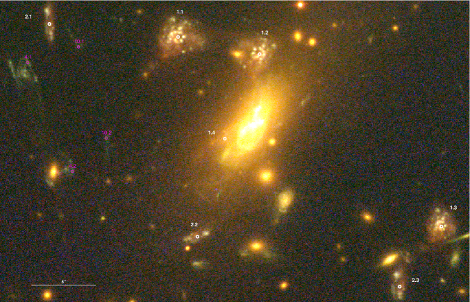
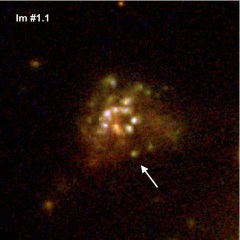
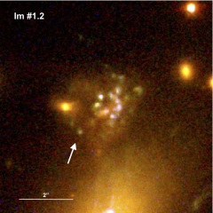
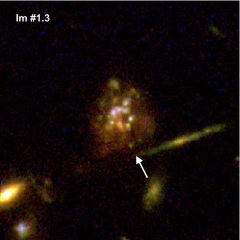
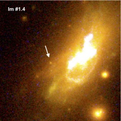
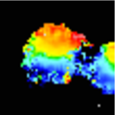
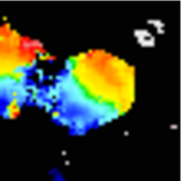
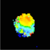
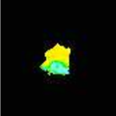
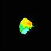
Figure 1: Top panel: Zoom into the core of MACS J0417. We here show a colour composite image from HST/ACS and WFC3/UVIS images. The white circles highlight the multiple images of systems #1 and #2 spectroscopically confirmed by our VLT/MUSE observations. North is up, East if left, and magenta circles show the other multiply-imaged systems visible in this field of view. Second panel: HST colour composite stamps of all four images of system #1, also nicknamed The Doughnut. We highlight with an arrow the part of The Doughnut that is quadruply-imaged. Third panel: MUSE low-resolution [OII] velocity maps of the four images of system #1. The stamps are the same size as the HST ones and cover a velocity range of -1500 to +1500 km.s^-1 and are fit above a threshold of 6$\sigma$ in bins averaged over 0.6″in size. Note the line emission of other images appear in the margin of each image apart from #1.3 which is the most isolated. Bottom panel: The velocity maps extracted from fitting the SINFONI spectra on the spaxel scale. The range in velocity is consistent with that recovered in the SINFONI observation when the poorer surface brightness sensitivity in the NIR is considered. The scale given on the HST stamp of image #1.2 is applicable to all other HST, MUSE, and SINFONI stamps.

2.2 Hubble Space Telescope

MACS J0417 was first observed with HST using the Wide-Field Planetary Camera 2 (WFPC2) in 2008 as part of the MACS SNAPshot programme G0-11103 (PI: Ebeling) in the F814W and F606W passbands . It was then observed with the Advanced Camera for Survey (ACS) in the F814W passband, and with the Wide Field Camera 3 (WFC3) through its UVIS channels in the F606W passband in 2010 (PI: von der Linden, G0-12009). It was subsequently observed in 2015 with ACS in the F435W passband, and with WFC3 in the F105W, F125W, 140W and F160W passbands as part of the RELICS programme (PI: Coe, GO-14096). Table 4 gives a summary of the HST observations available for MACS J0417.

For the analysis presented here, we make use of the publicly available RELICS data products. Observations with ACS and WFC3 were aligned and combined following the procedure described by Cerny et al. (2018); we used both 0.03″and 0.06″pixel-size images. The top panel of Fig. 1 shows a zoomed view of the central region of MACS J0417 as observed by HST; highlighted in white are two lensed systems spectroscopically confirmed by VLT/MUSE as listed in Table 5.

Table 4: Overview of the different HST observations of MACS J0417 as described in Sect. 2.2 including exposure time and date of observations for each filter and observing programme.

Camera/Filter	Exp. Time	Date	Prog. ID
	($s$)
WFPC2/F814W	1200	2007-11-21	11103
WFPC2/F606W	1200	2007-11-21	11103
ACS/F814W	1910	2010-12-10	12009
WFC3-UVIS/F606W	5364	2011-01-20	12009
WFC3-UVIS/F606W	1788	2011-02-28	12009
ACS/F435W	2000	2016-11-30	14096
WFC3/F105W	356	2016-02-11	14096
WFC3/F105W	756	2017-02-10	14096
WFC3/F125W	381	2016-12-30	14096
WFC3/F125W	356	2017-02-11	14096
WFC3/F140W	381	2016-12-30	14096
WFC3/F140W	356	2017-02-10	14096
WFC3/F160W	1006	2016-12-30	14096
WFC3/F160W	1006	2017-02-11	14096

2.3 Chandra X-ray Observatory

MACS J0417 was observed by the Chandra X-ray Observatory on three occasions (OBSID 3270, 11759, and 12010), for a total exposure time of 81.5 ks. All observations were performed with ACIS-I. We retrieved the data directly from the Chandra archive, as reduced with the ciao v4.10 pipeline. We did not reprocess the data and used the full-band images with no energy filter applied.

2.4 VLT/SINFONI

An archival VLT/SINFONI observation that covers two of the multiple images of system #1 (1.1 and 1.2 as listed in Table 5) was obtained as part of a survey of six lensed $0.7<z<1.1$ galaxies (087.A-0700(A), PI Limousin) on 2011 September 10 with the $J$-band grating and largest field mode of 8.0″$\times$ 8.0″. The spectral resolution in the $J$-band band is $\lambda/\Delta\lambda\sim$4500. Each observing block (OB) was taken in an ABBA observing pattern (A=Object frame, B=Sky frame) with chops to sky to allow improved sky subtraction. The target was observed for a total of 2.7 ks comprising nine individual exposures of 300 s in $\sim$0.6″seeing and photometric conditions. The observations were dithered and nodded to a sky position. The data were reduced using the ESORex pipeline to extract, wavelength calibrate, and flat field each spectrum and form a data cube. The final cube was generated by aligning the individual observations and then median combining them; 3$\sigma$ clipping was applied to reject cosmic rays. The seeing during these observations was insufficient to resolve the individual knots in system #1 but the overall velocity structure is well sampled.

The lower panel of Fig. 1 shows the velocity maps extracted from fitting these spectra on the spaxel scale. The H$\alpha$ and [NII] line complex is clearly detected; we measure a velocity gradient of -50 to +90 km s^-1 is recovered.

3 Strong-Lensing Mass Model

Table 5: Multiply imaged systems considered in this work, i.e. the (gold + sylver) set from Mahler et al. (2018a). The different star formation knots used as constraints for system #1 and system #2 are also highlighted on HST colour composite stamps in Fig. 5. The flux magnification factors come from our best-fit mass model, with errors derived from MCMC sampling. Redshifts with error bars correspond to values estimated by our model, errors come from MCMC sampling.

ID	R.A.	Dec	$z$	$\mu$
	($deg$)	($deg$)
1a.1	64.39615785	-11.90676027	0.8718	$5.4\pm 1.8$
1a.2	64.39431017	-11.90713584	0.8718	$3.9\pm 1.5$
1a.3	64.39034846	-11.91086438	0.8718	$2.5\pm 1.0$
1b.1	64.3960815	-11.90725472	0.8718	$7.1\pm 2.1$
1b.2	64.39472869	-11.9075832	0.8718	$4.0\pm 1.5$
1b.3	64.39029891	-11.91127399	0.8718	$2.3\pm 0.9$
1b.4	64.3949866	-11.90892984	0.8718	–
1c.1	64.39636429	-11.90698317	0.8718	$5.2\pm 1.8$
1c.2	64.39437083	-11.9074093	0.8718	$4.0\pm 1.5$
1c.3	64.39048794	-11.911052	0.8718	$2.5\pm 0.9$
1m.1	64.39616667	-11.90692935	0.8718	$5.7\pm 1.9$
1m.2	64.39443065	-11.90727847	0.8718	$4.9\pm 1.7$
1m.3	64.3903625	-11.91101333	0.8718	$2.4\pm 0.9$
2a.1	64.39909584	-11.90636889	1.0460	$2.6\pm 1.0$
2a.2	64.39556667	-11.91118194	1.0460	$2.5\pm 1.0$
2a.3	64.39137084	-11.91207389	1.0460	$3.1\pm 1.2$
2b.1	64.39899999	-11.9066325	1.0460	$2.7\pm 1.1$
2b.2	64.39582084	-11.91122639	1.0460	$2.5\pm 1.0$
2b.3	64.3912625	-11.91232361	1.0460	$2.9\pm 1.2$
2c.1	64.39900417	-11.90685487	1.0460	$2.8\pm 1.1$
2c.2	64.39595416	-11.91129862	1.0460	$2.5\pm 1.0$
2c.3	64.39129999	-11.91249333	1.0460	$2.8\pm 1.1$
3.1	64.39318	-11.901537	1.0460	$6.0\pm 1.9$
3.2	64.390026	-11.903434	1.0460	$10.4\pm 2.5$
3.3	64.388304	-11.905013	1.0460	$7.6\pm 2.2$
4.1	64.39952083	-11.90747917	$2.7\pm 0.2$	$6.5\pm 2.0$
4.2	64.39852916	-11.90983889	–	$2.5\pm 1.0$
4.3	64.38609459	-11.9153594	–	$2.1\pm 0.8$
5.1	64.379941	-11.897906	$2.0\pm 0.2$	$5.2\pm 1.8$
5.2	64.38237	-11.896413	–	$7.6\pm 2.2$
5.3	64.388438	-11.89163	–	$3.7\pm 1.4$
6.1	64.379991	-11.897349	$2.0\pm 0.2$	$6.5\pm 2.0$
6.2	64.381808	-11.89639	–	$3.2\pm 1.3$
6.3	64.388558	-11.89117	–	$3.4\pm 1.3$
8.1	64.388372	-11.894492	$2.3\pm 0.4$	$14.7\pm 2.9$
8.2	64.386885	-11.895489	–	$18.8\pm 3.2$
9.1	64.382068	-11.899994	$7.6\pm 0.5$	–
9.2	64.382338	-11.899779	–	$>20$
10.1	64.39839707	-11.9071427	$2.4\pm 0.4$	$8.4\pm 2.3$
10.2	64.39778511	-11.90911404	–	$5.3\pm 1.8$
11.1	64.40154413	-11.91891178	$5.3\pm 0.7$	$>20$
11.2	64.39970821	-11.92009933	–	$>20$
12.1	64.396902	-11.897085	$3.4\pm 0.5$	$2.4\pm 0.9$
12.2	64.38864	-11.9013	–	$2.6\pm 1.0$
12.3	64.383172	-11.906519	–	$2.9\pm 1.1$
13.1	64.397312	-11.897068	$3.6\pm 0.5$	$2.3\pm 0.9$
13.2	64.38842	-11.901684	–	$2.6\pm 1.0$
13.3	64.38349928	-11.9064465	–	$3.1\pm 1.2$
15.1	64.378193	-11.89451	$1.8\pm 0.2$	$5.4\pm 1.8$
15.2	64.38189	-11.892331	–	$7.8\pm 2.2$
15.3	64.385361	-11.890071	–	$5.6\pm 1.9$
16.1	64.385599	-11.886984	$3.2\pm 0.8$	$3.3\pm 1.3$
16.2	64.380143	-11.888425	–	$1.5\pm 0.5$
16.3	64.376525	-11.89254	–	$5.4\pm 1.8$
17.1	64.388212	-11.895269	$2.2\pm 0.4$	$>20$
17.2	64.387833	-11.895536	–	$>20$

3.1 Multiple images

Mahler et al. (2018a) identified 57 multiple images (in 17 families) in the cluster core. They classified each image as gold, silver or bronze following a similar process as for the Hubble Frontier Fields (HFF, Lotz et al., 2017): (i) gold images have spectroscopic redshifts, (ii) silver images are securely identified through their geometry, colour, and morphology, and (iii) bronze images are tentative identifications, some of which are based solely on predictions from the mass model. In this analysis, we restrict ourselves to the (gold + silver) set, which consists of 15 systems comprising 41 individual images. We refer to this mulitple image set as silver for the rest of the paper. IDs, coordinates, and redshifts for these multiple images are listed in Table 5. Note that, for systems #1 and #2, images are decomposed into several star-formation knots as shown in Appendix A (Fig. 5). As a result, we are using a total of 56 strong-lensing constraints.

Redshift constraints –

From the MUSE observations we obtain a spectroscopic redshift confirmation for 3 systems (systems #1, #2, and #3). All four multiple images of system #1, nicknamed The Doghnut, are spectroscopically confirmed at $z=0.8718$. The spectra of the three most prominent images of system #1 all show strong [OII], H$\beta$, H$\gamma$, H$\epsilon$ and H$\delta$ emission lines and MgII and Fe absorption lines in the UV. HST and MUSE stamps are shown in the middle panel of Fig. 1. The MUSE spectroscopic measurement is in good agreement with the Mahler et al. (2018a) LDSS3 spectroscopic redshift obtained at the Magellan Clay telescope (PI: Sharon) of $z=0.871$ for image 1.3 but with substantially better spectral resolution. The third row of Fig. 1 shows the MUSE velocity maps for all four images of system #1 extracted by fitting the [OII] doublet directly, which can be compared to the high resolution SINFONI velocity maps calculated from fits to the [NII] and H$\alpha$ complex shown in the bottom row of Fig. 1. The orientation of the observed rotation in the MUSE and SINFONI velocity maps is perpendicular to the critical line so the velocity maps appear to be very similar but one should note the low resolution MUSE velocity map of the third image (third stamp on third row of Fig. 1) shows a different axis of rotation as expected from the lensing configuration.

System #2 is composed of three multiple images, all spectroscopically confirmed at $z=1.046$ with strong [OII] and weak stellar absorption lines of the galaxy. All three images of system #3 are also spectroscopically confirmed by MUSE at $z=1.046$ but due to the faint nature of this arc only [OII] is detected. As one can notice systems #2 and #3 are both at the same redshift. We discuss this in more details in Appendix B. Finally we could not measure a secure redshift for system #4, either $z=2.7$ or $z=3.1$ depending on the spectral feature associated with the deepest absorption line at 5720Å. We discuss the case of system #4 in more detial in Sect. 4.3. Top panel of Fig. 1 shows a zoom into the core of MACS J0417, highlighting the geometrical configuration of system #1 and system #2 around the BCG.

The fourth image of The Doghnut –

MUSE observations also reveal a fourth image for system #1 which stands behind the brightest cluster galaxy (BCG), and thus is difficult to identify on the HST imaging as shown in the second row of Fig. 1. However, this image is partial, meaning only a part of The Doghnut is being quadruply-imaged by the cluster. We include this fourth component of system #1 in our mass model, and discuss its implications on the best-fit mass model in Sect. 4.2.

Table 6: PIEMD best-fit parameters for all three models that we run: the Fiducial Model, the Variation 1 Model and the Variation 2 Model. $DM1$ refers to the main cluster halo, and $DM2$ and $DM3$ to the North and North West group-scale halos respectively. We refer to the BCG of the main cluster halo as $BCG1$, and to the massive ellipticals at the center of the North and North West group-scale halos as $BCG2$ and $BCG3$ respectively. For the scaling relation, the reference magnitude is $mag_{\rm F814W}=19.45$. ^a Coordinates are given in arcseconds relative to the reference coordinate point: ($\alpha=64.394552$, $\delta=-11.908871$). ^b As explained in Sect. 3.3, ellipticity ($e$) is defined to be $(a^{2}-b^{2})/(a^{2}+b^{2})$, where $a$ and $b$ are the semi-major and semi-minor axes of the ellipse. ^c The position angle $\theta$ is given in degrees and is defined as the direction of the semi-major axis of the iso-potential, counted counterclockwise from the horizontal axis (being the R.A. axis).

Model name	Component	$\Delta$x${}^{\rm~{}a}$	$\Delta$y${}^{\rm~{}a}$	$e^{\rm~{}b}$	$\theta^{\rm c}$	$\sigma$	rcut	rcore
(Fit statistics)	–	(″)	(″)		($\deg$)	(km.s-1)	(kpc)	(kpc)
Fiducial Model	DM #1	0.7${}^{+0.4}_{-0.4}$	0.4${}^{+0.8}_{-0.6}$	0.72$\pm$0.03	55.2${}^{+0.5}_{-0.6}$	1033${}^{+27}_{-22}$	[1000.0]	14.9${}^{+0.7}_{-0.8}$
	DM #2	44.4${}^{+0.9}_{-2.0}$	71.8${}^{+1.0}_{-1.6}$	0.67$\pm$0.05	44.2${}^{+8.3}_{-5.5}$	499${}^{+121}_{-28}$	[1000.0]	11.0${}^{+6.4}_{-1.5}$
	DM #3	47.1${}^{+2.6}_{-0.1}$	46.8${}^{+0.8}_{-0.9}$	0.53$\pm$0.09	33.9${}^{+14.4}_{-14.6}$	426${}^{+33}_{-55}$	[1000.0]	12.5${}^{+2.0}_{-3.8}$
	BCG #1	[0.0]	[0.1]	[0.64]	[60.5]	418${}^{+19}_{-13}$	31.1${}^{+14.5}_{-9.1}$	[0.5]
	BCG #2	[47.8]	[69.6]	[0.35]	[74.1]	311${}^{+26}_{-39}$	102.3${}^{+5.0}_{-20.5}$	[0.3]
	BCG #3	[46.9]	[48.4]	[0.16]	[50.6]	269${}^{+41}_{-15}$	66.8${}^{+10.4}_{-13.2}$	[0.0]
	$L^{*}$ Galaxy	–	–	–	–	209${}^{+45}_{-27}$	15.5${}^{+24.7}_{-3.3}$	–
Variation 1 Model	DM #1	1.3${}^{+0.3}_{-0.5}$	1.3${}^{+0.5}_{-0.7}$	0.73$\pm$0.03	54.7${}^{+0.7}_{-0.5}$	1001${}^{+15}_{-19}$	[1000.0]	17.2${}^{+0.4}_{-2.1}$
	DM #2	47.1${}^{+0.9}_{-0.7}$	74.6${}^{+2.0}_{-1.0}$	0.64$\pm$0.11	45.7${}^{+4.9}_{-7.3}$	561${}^{+58}_{-60}$	[1000.0]	16.5${}^{+0.7}_{-1.8}$
	DM #3	46.2${}^{+2.9}_{-1.6}$	44.8${}^{+2.0}_{-1.7}$	0.42$\pm$0.08	34.5${}^{+17.2}_{-11.8}$	439${}^{+50}_{-41}$	[1000.0]	12.7${}^{+1.7}_{-2.4}$
	BCG #1	[0.0]	[0.1]	[0.64]	[60.5]	473${}^{+13}_{-37}$	67.6${}^{+2.8}_{-16.1}$	[0.5]
	BCG #2	[47.8]	[69.6]	[0.35]	[74.1]	305${}^{+21}_{-50}$	64.1${}^{+8.7}_{-27.8}$	[0.3]
	BCG #3	[46.9]	[48.4]	[0.16]	[50.6]	247${}^{+34}_{-12}$	17.2${}^{+13.9}_{-9.9}$	[0.0]
	$L^{*}$ Galaxy	–	–	–	–	209${}^{+39}_{-34}$	12.3${}^{+14.1}_{-12.6}$	–
Variation 2 Model	DM #1	0.1${}^{+0.4}_{-0.5}$	-0.2${}^{+0.5}_{-0.5}$	0.69$\pm$0.03	54.2${}^{+0.5}_{-0.4}$	981${}^{+16}_{-28}$	[1000.0]	14.4${}^{+1.0}_{-1.5}$
	DM #2	44.7${}^{+2.2}_{-1.1}$	69.4${}^{+1.9}_{-0.9}$	0.75$\pm$0.09	45.0${}^{+4.0}_{-13.4}$	570${}^{+51}_{-101}$	[1000.0]	17.3${}^{+0.1}_{-1.7}$
	DM #3	46.3${}^{+0.9}_{-1.2}$	53.5${}^{+1.2}_{-2.4}$	0.74$\pm$0.13	53.7${}^{+4.9}_{-7.0}$	397${}^{+113}_{-33}$	[1000.0]	13.9${}^{+4.3}_{-2.0}$
	BCG #1	[0.0]	[0.1]	[0.64]	[60.5]	417${}^{+21}_{-16}$	85.2${}^{+2.9}_{-13.5}$	[0.5]
	BCG #2	[47.8]	[69.6]	[0.35]	[74.1]	375${}^{+32}_{-21}$	98.2${}^{+10.4}_{-31.7}$	[0.3]
	BCG #3	[46.9]	[48.4]	[0.16]	[50.6]	276${}^{+16}_{-22}$	25.3${}^{+18.5}_{-12.4}$	[0.0]
	$L^{*}$ Galaxy	–	–	–	–	88${}^{+28}_{-27}$	89.2${}^{+9.9}_{-56.7}$	–

Table 7: Figures of merit for each model considered in Sect. 4.2. Columns show the Bayesian evidence ($\log{E}$) and likelihood ($\log{\mathcal{L}}$), the rms deviation of predicted multiple-image positions from their observed positions in the image plane, $rms$, the reduced $\chi^{2}$, $\chi_{red}^{2}$, the Bayesian Information Criterion, BIC, the Akaike Information Criterion, AIC, and the corrected AIC, AICc. We also quote the improvement on several parameters compare to the fiducial model: on the the BIC, $\delta_{\rm BIC}$, and the AICc, $\delta_{\rm AICc}$. A value of $\delta_{\rm BIC}$ and $\delta_{\rm AICc}$ greater than 10 reflects a significant improvement/degradation of the model compare to the fiducial one.

Model	$\log{E}$	$\log{\mathcal{L}}$	$rms$	$\chi^{2}_{\rm red}$	BIC	AIC	AICc	$\delta_{\rm BIC}$	$\delta_{\rm AICc}$
Fiducial Model	-104	-41	0.38″	0.9	262	158	198	–	–
Variation 1 Model	-110	-38	0.34″	0.8	254	151	192	8	6
Variation 2 Model	-117	-48	0.45″	1.3	271	171	209	-9	-11

3.2 Methodology

To model the mass distribution of MACS J0417 we use the lenstool software (Jullo et al., 2007). Our method closely follows the method used in previous works (Jauzac et al., 2014, 2015, 2016a) so we here only give a brief summary of the different steps in the build-up of the mass model. We refer the reader to Kneib et al. (1996), Smith et al. (2005), and Richard et al. (2011); Richard et al. (2014) for more details.

Our mass model combines large-scale dark matter halos to model the cluster components, and small-scale dark matter halos to model the cluster galaxies, typically large ellipticals (like the BCG) and galaxies in the proximity of multiple-images. All mass components are modelled as Pseudo Isothermal Elliptical Mass Distribution (PIEMD, Limousin et al., 2005; Elíasdóttir et al., 2007), parametrized by a position ($x$,$y$), an ellipticity ($e$), a position angle ($\theta$), a velocity dispersion ($\sigma$), a core radius ($r_{\rm core}$), and a cut radius ($r_{cut}$). For the PIEMDs used to model small-scale mass perturbers, cluster galaxies, we fix the parameters ($x$,$y$), $e$, and $\theta$, at the values measured from their light distribution (Kneib et al., 1996; Limousin et al., 2007b; Richard et al., 2014) and assume a Faber-Jackson empirical scaling relation (Faber & Jackson, 1976) to relate their velocity dispersion and cut radius to their observed luminosity (Jauzac et al., 2016a). We optimize the velocity dispersion and the cut radius for an $L^{\ast}$ galaxy only with $mag_{0}=19.45$ in the ACS/F814W passband. The velocity dispersion is allowed to vary between 20 and 220 km.s^-1, and the cut radius between 1 and 100 kpc. The r_cut upper limit is there to account for tidal stripping of galactic dark matter halos (Limousin et al., 2007a; Limousin et al., 2009; Natarajan et al., 2009; Wetzel & White, 2010). With such a parametric approach, dark matter halos are not allowed to contain zero mass, and hence we measure the goodness of our model to meet the observational constraints with the $\chi^{2}$ and rms statistics. The rms is measured as the difference between the observed position of the multiple images and the predicted position from the model. In principle, a low rms would indicate a better model (see Sect. 4.3).

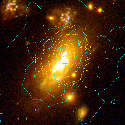
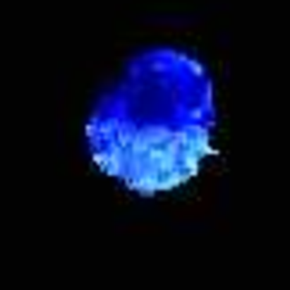
Figure 2: Left panel: HST colour composite stamp centered on the BCG. Cyan contours show the X-ray gas distribution from Chandra. Yellow contours show the [OII] emission of the BCG. The cyan and red crosses highlight the gas peak from the X-ray and the dark matter peak from the lensing analysis respectively. One will note the [OII] emission peak is consistent with the gas peak from the X-ray. The stamp is 15″$\times$15″. Right panel: MUSE low-resolution [OII] velocity map of the BCG. The stamp size is the same as the left panel and covers a velocity range of -450 to +450 km.s^-1. There is a significant blueshift to the optical line emission with gas velocities ranging from -50 to -450 km.s^-1, and a prominent velocity gradient across the system along the major axis of the BCG.

3.3 Results

Our final mass model includes three cluster-scale halos. MACS J0417 is a dynamically active cluster, which can be separated into three main components: the main halo located around the BCG ($\alpha=64.394552$, $\delta=-11.908871$), and two other group-scale halos located North ($\alpha=64.380985$, $\delta=-11.889541$, and North West ($\alpha=64.381231$, $\delta=-11.895417$) of the main cluster. Both group-scale halos have an over-density of cluster members located in their surroundings with a bright elliptical galaxy at their centre. For all three large-scale halos, we allow their positions to vary within 10″of their associated light peak, and their core radius between 1 and 20″. The velocity dispersion of the main halo can vary between 500 and 2 000 km.s^-1, and the velocity dispersion of the group-scale halos between 200 and 1 000 km.s^-1. The ellipticity, defined as $e=(a^{2}-b^{2})/(a^{2}+b^{2})$, and position angle of all three are also free parameters during the optimization process. The cut radius for all three is fixed to 1 000 kpc as strong-lensing constraints alone cannot probe the outer regions of the dark matter potential. Additionally, we include 177 mass perturbations induced by cluster galaxies by assigning to them a galaxy-scale halo following the method presented in Sect. 3.2 (Richard et al., 2014). Finally, we add three galaxy-scale halos to model the BCG and the two ellipticals at the centre of the main, North and North-West large-scale halos respectively for which we optimize both their cut radius and velocity dispersion. Using the 56 multiple images presented in Sect 3.1 and listed in Table 5, we optimize the above-mentioned free parameters of our mass model using lenstool. The redshift parameter of each multiply-imaged system without a spectroscopic measurement was set as a free parameter, and allowed to vary between 0.6 and 9.

The best-fit mass model optimized in the image plane gives us a rms of 0.38″and a reduced $\chi^{2}$ of 0.9. The best-fit redshifts for the multiple images and their estimated magnifications are given in Table 5. Our rms of 0.38″is similar to that obtained by Mahler et al. (2018a), 0.37″. This excellent agreement in terms of rms is encouraging as both teams have modeled the mass differently, i.e. using a different prior mass distribution with two more group-scale halo components to model the North and North West clumps, and adding the fourth partial image of The Doughnut on our side. The comparison between these two models is discussed in Sect. 4.4.

The best-fit parameters of our mass model are given in Table 6 under Fiducial Model. One will note that while all three dark matter large-scale halos are allowed to move around their light peak, both the main and the North West halos are well-aligned with their respective BCG as can be seen in Fig. 3 (dark matter peaks are highlighted with red crosses). However such good alignement between dark matter and light is not observed for the North halo. This could be due to several factors, such as the dynamical status of the cluster for example which is further discussed in Sect. 4.2. However even if we include the North and the North West components in our model, none of the multiply-imaged systems in their vicinities are spectroscopically confirmed. This implies the model in this region is degenerated and therefore any conclusion should be discussed with care concerning the dark matter centering of the North and North West clumps.

In order to provide a two-dimensional (cylindrical) mass of MACS J0417, we integrate the mass map within annuli centered on the main BCG. We measure a mass within 200 kpc of $M({\rm R<200\,kpc})=1.77\pm 0.03\,10^{14}\,{\rm M}_{\sun}$. The mass distribution obtained with this model is shown in Fig. 3 as white contours.

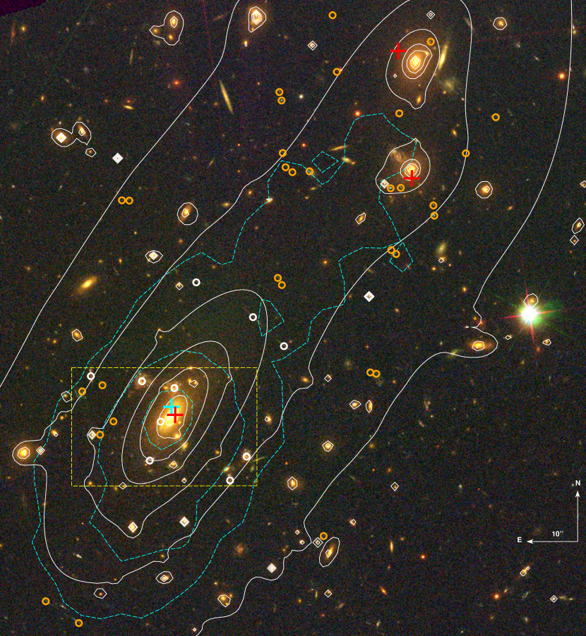
Figure 3: Colour composite image created from HST/ACS and WFC3/UVIS images in the F814W, F606W, and F435W passbands. Orange circles mark the positions of multiple images as listed in Table 5. White circles highlight multiple images spectroscopically confirmed in VLT/MUSE observations. Red crosses show the positions of the dark-matter clumps of the Fiducial Model, and the cyan cross is placed at the position of the X-ray peak. White and the dashed cyan contours show the distribution of mass reconstructed from our lensing mass model and gas from Chandra observations, respectively. The yellow box highlights the region visible in the top panel of Fig. 1. We find the main dark-matter halo to be well aligned with the light peak of the BCG, but offset with respect to both the peak of the X-ray surface brightness and the peak of the optical line emission from the BCG.

4 Discussion

4.1 The Brightest Cluster Galaxy

The most striking feature in MACS J0417 from the MUSE data is the disturbed BCG in the core of this cluster. It shows strong line emission (yellow contours in the left panel of Fig. 2) and significant H$\delta$ absorption consistent with the active star-formation first noted by Green et al. (2016). We see a significant spatial offset in the optical line emission from the stellar component of the BCG, $1.7\pm 0.5$″or 9.8$\pm 2.9$ kpc, that is consistent with the peak in the X-ray emission observed by Chandra. There is a significant blueshift to the optical line emission with gas velocities ranging from -50 to -450 km s^-1 and a prominent velocity gradient across the system along the major axis of the BCG that can be seen in the right panel of Fig. 2. Similar spatial and dynamical offsets in optical line emission have been seen in a number of other clusters (Hamer et al., 2012) that exhibit ‘sloshing’ activity, and the one observed here in MACS J0417 is the most distant example of this phenomenon. The direction of the ‘sloshing’ of the intra-cluster gas is consistent with the axis defined by the three mass components found in our lensing analysis and the more extended morphology of the cluster in the X-ray. Figure 3 shows the overall X-ray emission of the cluster as cyan contours, with the X-ray peak highlighted with a cyan cross. The dark matter peaks are shown as red crosses.

The fact that this offset gas cooling from the intra-cluster medium is coincident with the ionised cool gas points to direct deposition of cold molecular gas from the intra-cluster medium that is unrelated to the stellar population of the BCG. Therefore, in the cases where the X-ray peak is coincident with the BCG it is the cooling from the intra-cluster medium, and not stellar mass loss, that dictates the cold gas reservoir built up in the cluster core.

4.2 Dynamical History of MACS J0417

We aim at measuring precisely the dark matter peak location in the cluster core, compare it with its light and gas counterparts, confirm the dynamical history of the cluster core, and possibly put constraints on dark matter particle’s nature. We first estimate the improvement of our mass model when including the fourth partial multiple image of The Doghnut, and what it suggests about the dark matter centering in the main cluster halo. Adding to our Fiducial Model, we run a second mass model which does not include this partial fourth image of system #1, Variation 1 Model, but remains identical in terms of prior mass distribution: three large-scale dark matter halos, all three respective BCGs as well as 177 cluster galaxies. The best-fit parameters are given in Table 6.

Following the comparison method used by Acebron et al. (2017), Lagattuta et al. (2017), Mahler et al. (2018b), and Jauzac et al. (2018a), we measure three different Bayesian estimates to compare our two models, adding to the standard rms and reduced $\chi^{2}$: the Bayesian Information Criterion (BIC), the Akaike Information Criterion (AIC), and the Akaike Information Criterion corrected (AICc). The BIC is given by:

$${\rm BIC}=-2\log(\mathcal{L})+k\log(N)\ ,$$ (1)

where $N$ is the number of constraints and $k$ is the number of free parameters.

The Akaike Information Criterion can be calculated as:

$${\rm AIC}=-2\log(\mathcal{L})+2\ k\ ,$$ (2)

which is a more robust estimate of overfitting.

And finally the Akaike Information Criterion corrected is the AIC corrected for a finite number of free parameters:

$${\rm AICc}={\rm AIC}+\frac{2\ k\ (k+1)}{(N-k-1)}\ ,$$ (3)

For the BIC, the AIC, and the AICc, a penalty term for models with too many free parameters that overfit noise rather than capture additional information is included, which is larger with BIC and AICc than with AIC. Note that BIC, AIC and AICc were all developed for estimating the goodness of fits to models with linear parameters. As they provide us with an estimate, strong gravitational lensing is highly non-linear, thus these values should be interpreted with caution. For all these figures of merit, including the $\chi^{2}$ and the rms, lower values should be preferred. An improvement of less than 10 on the AICc should not be considered as statistically significant (Jauzac et al., 2018a). They are given for each model in Table 7. Improvement on all figures of merit between the Fiducial Model and Variation 1 Model are observed, however the improvement on the most reliable Bayesian estimator, the AICc, is less than 10, and is therefore considered as not statistically significant. However, the inclusion of this fourth image has a noticeable impact on the position on the dark matter peak.

The central region of the cluster core, where the BCG resides, is dominated by the stellar distribution, therefore constraining the exact location of the dark matter peak is extremely difficult and the error bars are usually large (can reach up to a few arcseconds) if we cannot add strong-lensing constraints in this region of the cluster or measure the stellar velocity dispersion of the BCG with high resolution as was done by Newman et al. (2011, 2013b); Newman et al. (2013a) and Monna et al. (2015, 2017). The geometry of system #1 is relatively common when looking at massive lenses, i.e. with a fourth radial image predicted in the central region (e.g. Sand et al., 2004; Sand et al., 2008). However due to the BCG being located in this region, it is difficult with usual optical data (HST in most cases) to identify this counterpart and locate it exactly, even with BCG subtraction methods as those usually leave residuals. Therefore, the centre of the dark matter halo is subject to large uncertainties.

In the case of MACS J0417, the MUSE data offer an opportunity to better constrain our mass model and precisely locate the main dark matter clump (DM #1 in Table 6) due to the identification of the fourth radial image of system #1. Our Fiducial Model predicts an alignment of $\pm$0.5″between the light peak (traced by the BCG) and the dark matter peak as shown in Fig. 3 (dark matter peaks are shown with red crosses). Such alignment is in good agreement with a cold dark matter (CDM; Peebles, 1984; Blumenthal et al., 1984) scenario where the dark matter potential is predicted to be cuspy, and light and dark matter are expected to ‘stick’ together. In a scenario where self-interacting dark matter were to be involved (SIDM; Spergel & Steinhardt, 2000), the dark matter potential is predicted to have a core, allowing the BCG to ‘slosh’ around, and therefore dark matter and light are not expected to ‘stick’ together anymore. Kim et al. (2017) demonstrated with SIDM simulations that offsets between light and dark matter peaks could reach up to a few hundred kpc. This was then observationally confirmed by Harvey et al. (2017). Therefore, measuring precisely the center of the dark matter potential and its offset with the light peak is one of the powerful tests that can be conducted in cluster cores to study the nature of dark matter (for more tests and investigations see Robertson et al., 2018). Our model without the fourth image (Variation 1 Model) predicts an offset between light and dark matter in the main potential (DM #1) of $1.3\pm 0.5$″, equivalent to an offset of $7.4\pm 2.9$ kpc, which could be interpreted as being in favour of a SIDM scenario (Massey et al., 2015, 2018). On the other side, our Fiducial Model predicts an offset of $0.5\pm 0.5$″, consistent with a perfect alignment, and thus in favour of a CDM scenario.

In order to push our investigation further, we look at all three main components of the cluster: dark matter, light and gas. The X-ray analysis with Chandra by Mann & Ebeling (2012) suggests that MACS J0417 has an ongoing merger event, its gas peak being misaligned with the light (Mann & Ebeling, 2012), with a gas plume in the direction of the NW halo as shown in Fig. 3 with the cyan contours, tracing a former interaction between the main and the North-West halos. The different components of MACS J0417 exhibit a familiar scenario observed in several other merging clusters such as the Bullet, the baby-bullet or Abell 2744 and MACS J0717 (Clowe et al., 2004; Bradač et al., 2006, 2008; Owers et al., 2011; Jauzac et al., 2016b; Ma et al., 2009; Jauzac et al., 2018b): dark matter and stars being aligned with the gas lagging behind. Such a situation represents another way to put constraints on dark matter’s nature. Merging clusters and in-falling substructures have often been used as ways to probe the nature of dark matter through its self-interaction cross-section (Kahlhoefer et al., 2014; Harvey et al., 2013). As these in-falling halos pass through the dense environment of another galaxy cluster the three components (gas, dark matter and galaxies) experience differential forces causing the dynamical behaviour of each component to change. The gas for example feels a large drag force as it interacts with the gaseous intra-cluster medium, the galaxies feel only the dynamical gravitational friction of the lumpy medium and the dark matter will behave according to its nature. Should dark matter have a significant self-interaction cross-section the halo will drag similarly to that of the gas, temporarily separating from the galaxies (Harvey et al., 2014; Robertson et al., 2017). Our analysis of MACS J0417 shows an offset between light and dark matter of the main cluster halo (DM#1) of $0.5\pm 0.5\arcsec$ and a gas offset of $1.7\pm 0.5\arcsec$. Adopting the method used in Harvey et al. (2015) and calibrated to simulations (Robertson et al., 2018, Harvey et al. in prep.) we can interpret this offset as caused by the particle properties of dark matter due to the former interaction between the main halo and the North-West halo of MACS J0417. After mass matching the simulations we find that the observed separation implies a cross-section upper-limit $\sigma_{\rm DM}/m<3$ cm².g^-1 consistent with other observations (e.g. Bradač et al., 2008; Dawson et al., 2012).

However, if we consider the significant offset in the optical emission line associated with the star-forming BCG in this cluster, and discussed in Sect. 4.1, we conclude that the observed offset between the gas and light/dark matter peaks in the main halo of MACS J0417 can be explained without including another possible dark matter candidate such as SIDM, which is in good agreement with the constraints we put on its self-interaction cross-section.

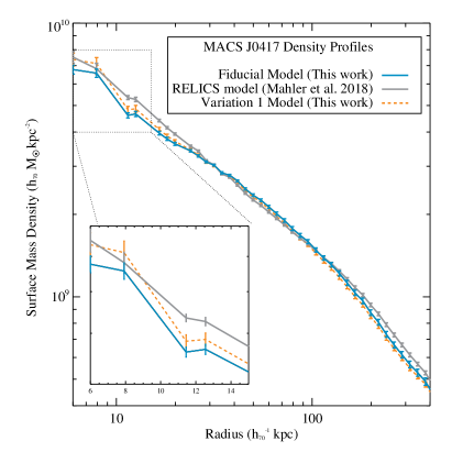
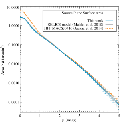
Figure 4: Left panel: 2D-density profiles obtained from our Fiducial Model in cyan, from the RELICS analysis from Mahler et al. (2018a) in grey, and from our Variation 1 Model in orange. One can see a really good agreement between all three models. The slight differences in the core is attributed to the presence of the fourth partial image of system #1 on our side, better constraining the inner most $\sim$10 kpc of the dark matter density profile. The inset plot zooms onto the 6-15 kpc region of the density profiles. Right panel: Surface area in the source plane covered by the overlap between ACS and WFC3 at a magnification above a given threshold $\mu$ for the present model in cyan, and the RELICS model presented in our companion paper by Mahler et al. (2018a) in grey. When put in perspective of MACS J0416 (orange dotted line), one of the HFF clusters, one can see that MACS J0417 has a high lensing power.

4.3 The impact of the redshift of system #4

Our Fiducial Model does not include the redshift of system #4 as its measurement from the MUSE data cube is uncertain as discussed in Sect. 3.1. As explained in Sect. 3.2, multiply-imaged systems without a spectroscopic confirmation have their redshift being optimized. The best-fit redshifts are given in Table 5. We do not use any photometric redshift prior, and for all systems without a spectroscopic redshift we let the redshift vary between 1 and 9 during the lenstool optimization. In the case of system #4, one can see that our Fiducial Model favors the 2.7 spectroscopic measurement, with a best-fit redshift of $2.7\pm 0.2$ (also in agreement with Variation 1 Model which gives an optimized redshift of $2.8\pm 0.2$).

As a matter of check, we run another model which now includes a redshift of 2.7 for system #4. The best-fit parameters of the model are given in Table 6, and its figures of merit in Table 7 under Variation 2 model. This model is identical to our Fiducial Model, except we have now fixed the redshift of system #4 to 2.7. The model is actually degraded compared to our Fiducial Model: an increase of the rms of 0.08″, and an increase of the AICc of 11. The value of the $\delta_{\rm AICc}$ between our Fiducial Model and the Variation 2 Model is greater than 10 and is thus considered here as significant. Adding the redshift of system #4 means we remove a free parameter from the model, therefore lower its flexibility.

Johnson & Sharon (2016) studied the impact of the redshift information for multiple images on the resulting mass model. They showed that less flexible models (such as Variation 2 Model in this work) due to more constraints (the redshift of system #4 in our case) produce higher rms, and higher figures of merit in general as shown in Table 7, which indicates a degraded model fit compare to the Fiducial Model. However, the investigation from Johnson & Sharon (2016) shows that such models are usually better at predicting the locations of images across the whole image plane. The comparison between our Fiducial Model and Variation 2 Model agrees with the conclusions from Johnson & Sharon (2016) and highlights the fact that standard/linear bayesian estimators of fit goodness should be taken with caution when it comes to comparing strong-lensing mass models, in particular if they use different number of constraints..

4.4 Comparison with the Mahler et al. (2018a) mass model

We compare our aperture mass measured within 200 kpc to the one obtained by the RELICS team and presented in Mahler et al. (2018a). In this Section, we refer to the Fiducial Model as our model, and for the Mahler et al. (2018a) model we refer to their Silver Model. They measure a two dimensional integrated mass of $M({\rm R<200\,kpc})=1.78\pm 0.02\times 10^{14}\,{\rm M}_{\sun}$ which is in excellent agreement with our measurement of $M({\rm R<200\,kpc})=1.77\pm 0.03\times 10^{14}\,{\rm M}_{\sun}$.

The left panel of Fig. 4 shows the two dimensional density profiles obtained by our Fiducial Model in cyan, and by the Mahler et al. (2018a) model in grey. One can see that the two profiles exhibit a similar trend, with our model predicting a lower density in the core. The only difference between the two models in this region of the cluster is the inclusion of the fourth image of system #1, which is not included in the RELICS model. While the Mahler et al. (2018a) model predicts a fourth image for this system, its position cannot be unambiguously identified in the HST data alone.The fourth multiple image of The Doghnut is a radial pair merging on the critical curve, therefore it brings strong constraints on the inner density profile of the cluster potential ($<10$ kpc) as discussed in Sect. 4.2. In Fig. 4, we also plot the density profile we obtain with our Variation 1 Model in orange, which is identical to the Fiducial Model apart from the inclusion of the fourth image of system #1. One can see that the inner ($R>10$ kpc) density profile in this case is similar to the one obtained by Mahler et al. (2018a). We thus conclude that this additional constraint is responsible for the difference in shape of the inner density profile of MACS J0417.

The right panel of Fig. 4 shows the surface area in the source plane, $\sigma_{\mu}$, above a given magnification factor, $\mu$, for our Fiducial Model (cyan) and the RELICS model (grey) presented in our companion paper (Mahler et al., 2018a). This metric is a good estimator of the efficiency of the lensing configuration to magnify high-redshift galaxies as suggested initially by Wong et al. (2012), as $\sigma_{\mu}$ is directly proportional to the unlensed comoving volume covered at this magnification. We compute $\sigma_{\mu}$ for a source at $z=9$. It is calculated from the multiple image with the highest magnification at each source position. Mahler et al. (2018a) centered their analysis on a comparison of photometric and model-fitted redshifts as well as on the lensed high-redshift candidates for future follow-up with the James Web Space Telescope (JWST). We use this Section to demonstrate that even if our models are slightly different, the outputs are in extremely good agreement. Following our work on the Hubble Frontier Fields, we estimate the area above $\mu=3$ as our metric. We measure $\sigma(\mu>3)=0.22$ arcmin² and $\sigma(\mu>3)=0.23$ arcmin² for our Fiducial Model and the RELICS model respectively. These two values are in excellent agreement. Our measurement of $\sigma(\mu>3)$ can be put in perspective with the values obtained for some of the HFF clusters, i.e. 0.44 arcmin² for Abell 2744 (Jauzac et al., 2015), 0.26 arcmin² for MACS J0416.1-2403 (Jauzac et al., 2014). We show in the right panel of Fig. 4 the same relation but for MACS J0416 in orange. This strengthens the fact that MACS J0417 has a relatively high lensing power, and thus should be an interesting cluster to probe the high-redshift universe as stressed by Mahler et al. (2018a).

5 Conclusion

We present MUSE observations of the massive galaxy cluster MACS J0417.5-1154 at $z=0.441$, discovered in the MAssive Cluster Survey (MACS, Ebeling et al., 2001; Mann & Ebeling, 2012). The high mass and disturbed morphology of MACS J0417 make it a powerful gravitational lens. VLT/MUSE observations provide spectroscopic confirmation of three of the four high-confidence multiple-image families in the MUSE field of view: system #1 at $z=0.8718$, systems #2 and #3 at $z=1.046$, and system #4 at either $z=2.7$ or $z=3.1$, where the MUSE spectral range contains few strong lines. System #1 is of particular interest, as the MUSE observations provide us with the detection of a fourth radial image located behind the BCG, which would have been difficult to locate from imaging data alone (even at HST resolution), as the BCG’s high star-formation rate contaminates the bluer bands where the fourth image of system #1 is visible.

Based on the multiple images identified in our companion paper (Mahler et al., 2018a), we build a strong-lensing mass model including the MUSE redshifts and the fourth image of system #1, referred to as the Fiducial Model. Our best-fit mass model recovers the multiple-image positions with an rms of 0.38″and yields a two-dimensional enclosed mass of $M({\rm R<200\,kpc})=1.77\pm 0.03\times 10^{14}\,{\rm M}_{\sun}$. We then run a test model, called the Variation 1 Model, which does not include the central image of system #1. Unlike the Fiducial Model, the Variation 1 Model does not predict almost perfect alignment between the light peak of the BCG and the dark-matter peak. This difference highlights the impact and thus the importance of strong-lensing radial constraints for precise measurements of the location of the dark-matter peak in cluster cores. The good alignment of $(0.5\pm 0.5)$″ found by the Fiducial Model is consistent with a cold dark-matter scenario. The identification of this faint radial image also demonstrates the power of IFU instruments for such work, especially of MUSE which combines a large redshift range with a large field of view and a high spatial resolution.

Regarding gas distribution in MACS J0417, we use Chandra observations of our target to identify an offset with respect to the light/dark-matter peak of $1.7\pm 0.5$″. Following the method developed by Harvey et al. (in prep.) we derive from this offset an upper limit to the self-interaction cross-section of dark matter of $\sigma_{\rm DM}/m<3$ cm².g^-1, in good agreement with previous measurements. However, we note that the X-ray peak coincides with the optical emission-line peak of the BCG initially observed by Green et al. (2016), and confirmed by our MUSE observations. Using this information, we estimate that the gas-dark matter-light offset can be explained by the on-going merger event in this actively evolving system (Mann & Ebeling, 2012): during the collision with the North-Western subcluster, the gaseous intra-cluster medium was held back while the effectively non-collisional dark matter and main stellar components continued unimpeded on their trajectory, and it is the local concentration of cold gas that led to direct star formation at a location offset from the light peak of the BCG.

We also compares our mass model with the one from Mahler et al. (2018a) and find excellent agreement in terms of rms (they obtain an rms of 0.37″) and total mass ($M({\rm R<200\,kpc})=(1.78\pm 0.02)\times 10^{14}\,{\rm M}_{\sun}$). Since the two mass models were created independently, we investigate the differences between them in more detail by considering two different model outputs: (1) the two-dimensional density profile, and (2) the surface area in the source plane, $\sigma_{\mu}$, above a certain magnification $\mu$, which is a good estimator of the lensing power of a cluster. The two density profiles show a slight discrepancy in the inner region, $R<10$ kpc, which we attribute to the inclusion of the fourth image of system #1 in our model. The lensing power of MACS J0417 predicted by both our Fiducial Model and the model derived by Mahler et al. (2018a) is very similar; specifically, the two studies find $\sigma(\mu>3)=0.22$ arcmin² and $\sigma(\mu>3)=0.23$ arcmin², respectively. We note that these values are comparable to those previously measured by us for the HFF target MACS J0416.1-2403 ($\sigma(\mu>3)=0.26$ arcmin²; Jauzac et al., 2014), underlining that MACS J0417 is indeed a powerful lens and well suited to probe the high-redshift universe (see Mahler et al., 2018a, for more details).

The scientific efficiency of MUSE observations of massive clusters is especially high, as they allow the spectroscopic identification and charaterization of both numerous cluster members and strongly lensed background galaxies, soon resulting in a sample of dozens of spectroscopically selected lensed galaxies for the community to follow up with new facilities such as ALMA, JWST and SKA.

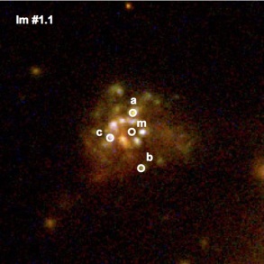
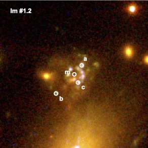
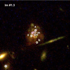
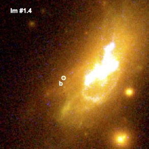
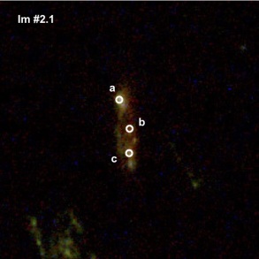
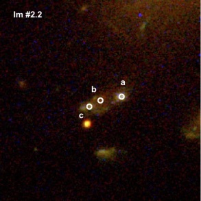
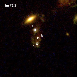
Figure 5: HST colour composite stamps of the four multiple images of system #1 (Top panel), and the three multiple images of system #2 (Bottom panel). White circles highlight the position of the star formations knots used in the mass modeling, as listed in Table 5. The size of the stamps is the same as in Fig. 1.

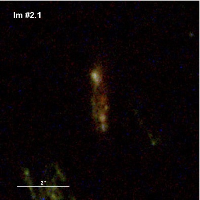
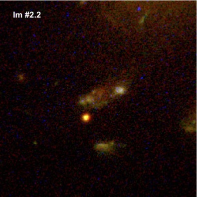
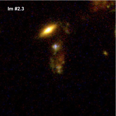
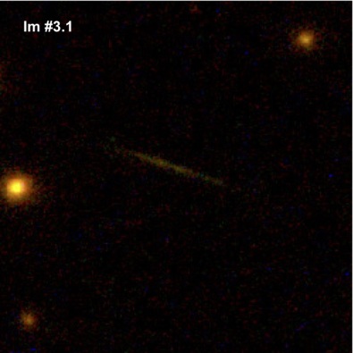
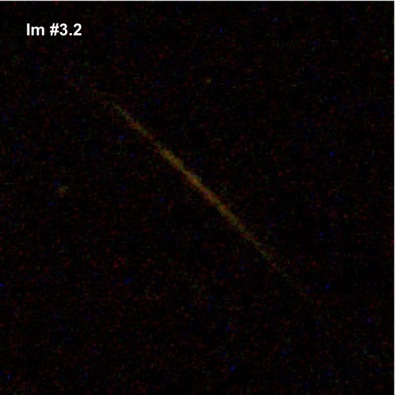
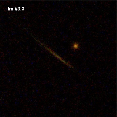
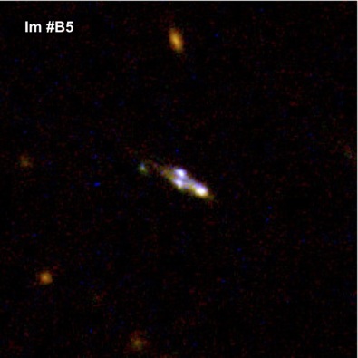
Figure 6: Galaxy triplet at $z=1.046$. The three stamps of the first and second raws show the three lensed images of system #2 and system #3 respectively from the HST colour composite image. The third row shows the third galaxy at $=1.046$ identified in the MUSE data cube, which is strongly lensed but not multiply-imaged as it appears in the HST colour composite image, the second stamp shows the source reconstruction. Source #2 and #3 are separated by 130.4 kpc, source #2 and source #B5 are separated by 154.1 kpc, and source #3 and source #B5 are separated by 284.3 kpc. Such separations imply this galaxy triplet is not interacting.

Appendix A Multiple images of systems #1 & #2

Figure 5 shows the different components in each multiple images of system #1 and system #2 used as constraints in our mass model presented in Table 5.

Appendix B A galaxy triplet at $z=1.046$

MUSE observations allowed us to measure the spectroscopic redshift of three multiply-imaged systems, two of which, system #1 and system #2, are at $z=1.046$. Adding to that, a third galaxy at $z=1.046$ is detected. This one is located outside the multiple image region, it is still relatively highly magnified, $\mu=6.2\pm 2.0$, but not multiply imaged. As our mass model allows us to retrace back into the source plane, we can thus investigate this coincidence of three galaxies at the same redshift, and for example identify any possible interactions. Fig. 6 shows the HST stamps of the three images of systems #2 and system #3, as well as of galaxy #B5.

From the lens model we can measure the position of all three galaxies in the source plane at $z=1.046$, and thus measure the distance between them. We give those distances both in arcseconds and kpc in Table 8. The multiply-imaged galaxies, galaxies #2 and #3 in Table 8, are separated by 130.4 kpc, while galaxy #2 is located at 154.1 kpc from galaxy #B5. Such large distances imply those three galaxies are not interacting at the moment, however they could be part of a background group or cluster at $z=1.046$. Their large separation does not imply they did not interact in the past.

In Table 8 we also give the distances measured by Mahler et al. (2018) in kpc for comparison. Both our models predict distances that are in excellent agreement. This independent result reinforces the discussion in Sect. 4.4 which concludes both models are giving extremely similar results.

Table 8: Distances between each galaxies part of the galaxy triplet detected in MUSE at $z=1.046$. At such redhsift, $1\arcsec=8.09$ kpc.

	$D_{\rm\#2-\#3}$	$D_{\rm\#2-\#B5}$	$D_{\rm\#3-\#B5}$
Fiducial Model	16.1″	19.1″	35.1″
	130.4 kpc	154.1 kpc	284.3 kpc
Mahler et al. 2018	131 kpc	157 kpc	288.6 kpc

Appendix C A dense starburst at $z=0.56$

One object detected in the MUSE field that stood out was object #B1 at $z=0.5635$ in Table 3 that is dominated by narrow [OIII] 4959 Å and 5007 Å with no detectable [OII] and H$\beta$ emission. The very high equivalent width of this source of $>150$ implies that it is an extreme starburst in the “Green Pea” class (Cardamone et al., 2009). These galaxies are rare as only two [OIII]-only emission galaxies were found in the first MUSE survey field in the HUDF out of 1338 sources (Inami et al., 2017). The HST imaging shows a compact but extended object with an AB magnitude of around 25.8 mag in the F814W filter so considering the likely line contamination in the band the stellar mass of the galaxy is likely to be below $10^{9}\,{\rm M}_{\sun}$. There is no significant X-ray emission from the source in the Chandra observation so the X-ray luminosity of the galaxy is $<2\times$10⁴² erg s^-1. It is also undetected in SPIRE at 250 $\mu$m from the Herschel Lensing Survey-snapshot project (Egami et al., 2010) giving an upper limit on star formation of $\sim 10\,{\rm M}_{\sun}$ yr^-1 so consistent with the observed specific star formation rates measured for these remarkable galaxies.

The implied amplification from our Fiducial Model for this galaxy, $\mu=1.4\pm 0.4$, is relatively low but the short lens to object distance is the dominant factor in this.

Determining the wider spectral properties of this intriguing source in the UV and NIR would be straightforward given the nature of the line emission and our larger MUSE survey and all other high Galactic latitude observations will reveal how unusual this class of emission line galaxy is.

References

- Acebron et al. (2017) Acebron A., Jullo E., Limousin M., Tilquin A., Giocoli C., Jauzac M., Mahler G., Richard J., 2017, MNRAS, 470, 1809
- Annunziatella et al. (2017) Annunziatella M., et al., 2017, ApJ, 851, 81
- Applegate et al. (2014) Applegate D. E., et al., 2014, MNRAS, 439, 48
- Atek et al. (2015) Atek H., et al., 2015, ApJ, 814, 69
- Atek et al. (2018) Atek H., Richard J., Kneib J.-P., Schaerer D., 2018, MNRAS, 479, 5184
- Bacon et al. (2010) Bacon R., et al., 2010, in Society of Photo-Optical Instrumentation Engineers (SPIE) Conference Series. p. 8, doi:10.1117/12.856027
- Bacon et al. (2016) Bacon R., Piqueras L., Conseil S., Richard J., Shepherd M., 2016, MPDAF: MUSE Python Data Analysis Framework, Astrophysics Source Code Library (ascl:1611.003)
- Bacon et al. (2017) Bacon R., et al., 2017, A&A, 608, A1
- Blumenthal et al. (1984) Blumenthal G. R., Faber S. M., Primack J. R., Rees M. J., 1984, Nature, 311, 517
- Bonamigo et al. (2018) Bonamigo M., et al., 2018, ApJ, 864, 98
- Bond et al. (1996) Bond J. R., Kofman L., Pogosyan D., 1996, Nature, 380, 603
- Botteon et al. (2018) Botteon A., Gastaldello F., Brunetti G., 2018, MNRAS, 476, 5591
- Bouwens et al. (2017a) Bouwens R. J., Illingworth G. D., Oesch P. A., Atek H., Lam D., Stefanon M., 2017a, ApJ, 843, 41
- Bouwens et al. (2017b) Bouwens R. J., Oesch P. A., Illingworth G. D., Ellis R. S., Stefanon M., 2017b, ApJ, 843, 129
- Bradač et al. (2006) Bradač M., et al., 2006, ApJ, 652, 937
- Bradač et al. (2008) Bradač M., Allen S. W., Treu T., Ebeling H., Massey R., Morris R. G., von der Linden A., Applegate D., 2008, ApJ, 687, 959
- Caminha et al. (2017a) Caminha G. B., et al., 2017a, A&A, 600, A90
- Caminha et al. (2017b) Caminha G. B., et al., 2017b, A&A, 607, A93
- Cardamone et al. (2009) Cardamone C., et al., 2009, MNRAS, 399, 1191
- Cerny et al. (2018) Cerny C., et al., 2018, ApJ, 859, 159
- Chirivì et al. (2018) Chirivì G., Suyu S. H., Grillo C., Halkola A., Balestra I., Caminha G. B., Mercurio A., Rosati P., 2018, A&A, 614, A8
- Clowe et al. (2004) Clowe D., De Lucia G., King L., 2004, MNRAS, 350, 1038
- Colless et al. (2001) Colless M., et al., 2001, MNRAS, 328, 1039
- Dawson et al. (2012) Dawson W. A., et al., 2012, ApJ, 747, L42
- Dayal & Ferrara (2018) Dayal P., Ferrara A., 2018, preprint, (arXiv:1809.09136)
- Dietrich et al. (2012) Dietrich J. P., Werner N., Clowe D., Finoguenov A., Kitching T., Miller L., Simionescu A., 2012, Nature, 487, 202
- Dwarakanath et al. (2011) Dwarakanath K. S., Malu S., Kale R., 2011, Journal of Astrophysics and Astronomy, 32, 529
- Ebeling et al. (2001) Ebeling H., Edge A. C., Henry J. P., 2001, ApJ, 553, 668
- Ebeling et al. (2010) Ebeling H., Edge A. C., Mantz A., Barrett E., Henry J. P., Ma C. J., van Speybroeck L., 2010, MNRAS, 407, 83
- Egami et al. (2010) Egami E., et al., 2010, A&A, 518, L12
- Elíasdóttir et al. (2007) Elíasdóttir Á., et al., 2007, preprint, 710 (arXiv:0710.5636)
- Faber & Jackson (1976) Faber S. M., Jackson R. E., 1976, ApJ, 204, 668
- Fumagalli et al. (2016) Fumagalli M., Cantalupo S., Dekel A., Morris S. L., O’Meara J. M., Prochaska J. X., Theuns T., 2016, MNRAS, 462, 1978
- Fumagalli et al. (2017) Fumagalli M., et al., 2017, MNRAS, 471, 3686
- Green et al. (2016) Green T. S., et al., 2016, MNRAS, 461, 560
- Grillo et al. (2015) Grillo C., et al., 2015, preprint, (arXiv:1511.04093)
- Hamer et al. (2012) Hamer S. L., Edge A. C., Swinbank A. M., Wilman R. J., Russell H. R., Fabian A. C., Sanders J. S., Salomé P., 2012, MNRAS, 421, 3409
- Harvey et al. (2013) Harvey D., Massey R., Kitching T., Taylor A., Jullo E., Kneib J.-P., Tittley E., Marshall P. J., 2013, MNRAS, 433, 1517
- Harvey et al. (2014) Harvey D., et al., 2014, MNRAS, 441, 404
- Harvey et al. (2015) Harvey D., Massey R., Kitching T., Taylor A., Tittley E., 2015, Science, 347, 1462
- Harvey et al. (2017) Harvey D., Courbin F., Kneib J. P., McCarthy I. G., 2017, MNRAS, 472, 1972
- Hoekstra et al. (2013) Hoekstra H., Bartelmann M., Dahle H., Israel H., Limousin M., Meneghetti M., 2013, Space Sci. Rev., 177, 75
- Inami et al. (2017) Inami H., et al., 2017, A&A, 608, A2
- Ishigaki et al. (2015) Ishigaki M., Kawamata R., Ouchi M., Oguri M., Shimasaku K., Ono Y., 2015, ApJ, 799, 12
- Ishigaki et al. (2018) Ishigaki M., Kawamata R., Ouchi M., Oguri M., Shimasaku K., Ono Y., 2018, ApJ, 854, 73
- Jauzac et al. (2012) Jauzac M., et al., 2012, MNRAS, 426, 3369
- Jauzac et al. (2014) Jauzac M., et al., 2014, MNRAS, 443, 1549
- Jauzac et al. (2015) Jauzac M., et al., 2015, MNRAS, 452, 1437
- Jauzac et al. (2016a) Jauzac M., et al., 2016a, MNRAS, 457, 2029
- Jauzac et al. (2016b) Jauzac M., et al., 2016b, MNRAS, 463, 3876
- Jauzac et al. (2018a) Jauzac M., Harvey D., Massey R., 2018a, MNRAS, 477, 4046
- Jauzac et al. (2018b) Jauzac M., et al., 2018b, MNRAS, 481, 2901
- Johnson & Sharon (2016) Johnson T. L., Sharon K., 2016, ApJ, 832, 82
- Jullo et al. (2007) Jullo E., Kneib J.-P., Limousin M., Elíasdóttir Á., Marshall P. J., Verdugo T., 2007, New Journal of Physics, 9, 447
- Kahlhoefer et al. (2014) Kahlhoefer F., Schmidt-Hoberg K., Frandsen M. T., Sarkar S., 2014, MNRAS, 437, 2865
- Karman et al. (2015) Karman W., et al., 2015, preprint, (arXiv:1509.07515)
- Kawamata et al. (2018) Kawamata R., Ishigaki M., Shimasaku K., Oguri M., Ouchi M., Tanigawa S., 2018, ApJ, 855, 4
- Kim et al. (2017) Kim S. Y., Peter A. H. G., Wittman D., 2017, MNRAS, 469, 1414
- Kneib & Natarajan (2011) Kneib J.-P., Natarajan P., 2011, A&ARv, 19, 47
- Kneib et al. (1996) Kneib J.-P., Ellis R. S., Smail I., Couch W. J., Sharples R. M., 1996, ApJ, 471, 643
- Lagattuta et al. (2017) Lagattuta D. J., et al., 2017, MNRAS, 469, 3946
- Limousin et al. (2005) Limousin M., Kneib J.-P., Natarajan P., 2005, MNRAS, 356, 309
- Limousin et al. (2007a) Limousin M., Kneib J. P., Bardeau S., Natarajan P., Czoske O., Smail I., Ebeling H., Smith G. P., 2007a, A&A, 461, 881
- Limousin et al. (2007b) Limousin M., et al., 2007b, ApJ, 668, 643
- Limousin et al. (2009) Limousin M., Sommer-Larsen J., Natarajan P., Milvang-Jensen B., 2009, ApJ, 696, 1771
- Livermore et al. (2017) Livermore R. C., Finkelstein S. L., Lotz J. M., 2017, ApJ, 835, 113
- Lotz et al. (2017) Lotz J. M., et al., 2017, ApJ, 837, 97
- Ma et al. (2009) Ma C.-J., Ebeling H., Barrett E., 2009, ApJ, 693, L56
- Mahler et al. (2018a) Mahler G., et al., 2018a, preprint, (arXiv:1810.13439)
- Mahler et al. (2018b) Mahler G., et al., 2018b, MNRAS, 473, 663
- Mann & Ebeling (2012) Mann A. W., Ebeling H., 2012, MNRAS, 420, 2120
- Massey et al. (2010) Massey R., Stoughton C., Leauthaud A., Rhodes J., Koekemoer A., Ellis R., Shaghoulian E., 2010, MNRAS, 401, 371
- Massey et al. (2015) Massey R., et al., 2015, MNRAS, 449, 3393
- Massey et al. (2018) Massey R., et al., 2018, MNRAS, 477, 669
- Monna et al. (2015) Monna A., et al., 2015, MNRAS, 447, 1224
- Monna et al. (2017) Monna A., et al., 2017, MNRAS, 465, 4589
- Natarajan et al. (2009) Natarajan P., Kneib J.-P., Smail I., Treu T., Ellis R., Moran S., Limousin M., Czoske O., 2009, ApJ, 693, 970
- Newman et al. (2011) Newman A. B., Treu T., Ellis R. S., Sand D. J., 2011, ApJ, 728, L39+
- Newman et al. (2013a) Newman A. B., Treu T., Ellis R. S., Sand D. J., Nipoti C., Richard J., Jullo E., 2013a, ApJ, 765, 24
- Newman et al. (2013b) Newman A. B., Treu T., Ellis R. S., Sand D. J., 2013b, ApJ, 765, 25
- Owers et al. (2011) Owers M. S., Randall S. W., Nulsen P. E. J., Couch W. J., David L. P., Kempner J. C., 2011, ApJ, 728, 27
- Pandge et al. (2018) Pandge M. B., Monteiro-Oliveira R., Bagchi J., Simionescu A., Limousin M., Raychaudhury S., 2018, MNRAS, p. 2802
- Parekh et al. (2017) Parekh V., Dwarakanath K. S., Kale R., Intema H., 2017, MNRAS, 464, 2752
- Peebles (1984) Peebles P. J. E., 1984, ApJ, 277, 470
- Postman et al. (2012) Postman M., et al., 2012, ApJS, 199, 25
- Richard et al. (2011) Richard J., Jones T., Ellis R., Stark D. P., Livermore R., Swinbank M., 2011, MNRAS, 413, 643
- Richard et al. (2014) Richard J., et al., 2014, MNRAS, 444, 268
- Richard et al. (2015) Richard J., et al., 2015, MNRAS, 446, L16
- Robertson et al. (2017) Robertson A., Massey R., Eke V., 2017, MNRAS, 465, 569
- Robertson et al. (2018) Robertson A., Harvey D., Massey R., Eke V., McCarthy I. G., Jauzac M., Li B., Schaye J., 2018, preprint, (arXiv:1810.05649)
- Salmon et al. (2017) Salmon B., et al., 2017, preprint, (arXiv:1710.08930)
- Sand et al. (2004) Sand D. J., Treu T., Smith G. P., Ellis R. S., 2004, ApJ, 604, 88
- Sand et al. (2008) Sand D. J., Treu T., Ellis R. S., Smith G. P., Kneib J.-P., 2008, ApJ, 674, 711
- Sandhu et al. (2018) Sandhu P., Malu S., Raja R., Datta A., 2018, Ap&SS, 363, 133
- Schaye et al. (2015) Schaye J., et al., 2015, MNRAS, 446, 521
- Schmidt et al. (2014) Schmidt K. B., et al., 2014, ApJ, 782, L36
- Schneider et al. (1992) Schneider P., Ehlers J., Falco E. E., 1992, Gravitational Lenses. Berlin: Springer-Verlag
- Smith et al. (2005) Smith G. P., Kneib J.-P., Smail I., Mazzotta P., Ebeling H., Czoske O., 2005, MNRAS, 359, 417
- Soto et al. (2016) Soto K. T., Lilly S. J., Bacon R., Richard J., Conseil S., 2016, MNRAS, 458, 3210
- Spergel & Steinhardt (2000) Spergel D. N., Steinhardt P. J., 2000, Physical Review Letters, 84, 3760
- Springel et al. (2005) Springel V., et al., 2005, Nature, 435, 629
- Treu et al. (2016) Treu T., et al., 2016, ApJ, 817, 60
- Vogelsberger et al. (2014) Vogelsberger M., et al., 2014, MNRAS, 444, 1518
- Weilbacher (2015) Weilbacher P., 2015, in Science Operations 2015: Science Data Management - An ESO/ESA Workshop, held 24-27 November, 2015 at ESO Garching. Online at <A href=“https://www.eso.org/sci/meetings/2015/SciOps2015.html”> https://www.eso.org/sci/meetings/2015/SciOps2015.html</A>, id.1. p. 1, doi:10.5281/zenodo.34658
- Wetzel & White (2010) Wetzel A. R., White M., 2010, MNRAS, 403, 1072
- Wong et al. (2012) Wong K. C., Ammons S. M., Keeton C. R., Zabludoff A. I., 2012, ApJ, 752, 104
- von der Linden et al. (2014) von der Linden A., et al., 2014, MNRAS, 439, 2