Overlapped Embedded Fragment Stochastic Density Functional Theory for Covalently Bonded Materials

Overlapped Embedded Fragment Stochastic Density Functional Theory for Covalently Bonded Materials

Abstract

The stochastic density functional theory (DFT) [Phys. Rev. Lett. 111, 106402 (2013)] is a valuable linear scaling approach to Kohn-Sham DFT that does not rely on the sparsity of the density matrix. Linear (and often sub-linear) scaling is achieved by introducing a controlled statistical error in the density, energy and forces. The statistical error (noise) is proportional to the inverse square root of the number of stochastic orbitals and thus decreases slowly, however, by dividing the system to fragments that are embedded stochastically, the statistical error can be reduced significantly. This has been shown to provide remarkable results for non-covalently bonded systems, however, the application to covalently bonded systems had limited success, particularly for delocalized electrons. Here, we show that the statistical error in the density correlates with both the density and the density matrix of the system and propose a new fragmentation scheme that elegantly interpolates between overlapped fragments. We assess the performance of the approach for bulk silicon of varying supercell sizes (up to $N_{e}=16384$ electrons) and show that overlapped fragments reduce significantly the statistical noise even for systems with a delocalized density matrix.

I Introduction

An accurate description of the electronic properties is often a prerequisite for understand the behavior of complex materials. Density functional theory (Hohenberg and Kohn, 1964) within the Kohn-Sham (KS) formulation (Kohn and Sham, 1965) provides an excellent framework that balances computational complexity and accuracy and thus, has been the method of choice for extended, large-scale systems. Solving the KS equations scales formally as $O\left(N_{e}^{3}\right)$ where $N_{e}$ is the number of electron in the system. Traditional implementations of KS-DFT are often limited to relatively systems containing $N_{e}<10^{4}$ electrons,(Baroni et al., 2001; Frauenheim et al., 2002; Freysoldt et al., 2014) even with the high-performance computer architectures of today. Clearly, there is a need for low-scaling KS-DFT approaches.

A natural approach to linear-scaling KS-DFT relies on the “locality” of the density matrix, that is, elements of the density matrix $\rho(\boldsymbol{r},\boldsymbol{r}^{\prime})$ decay with increasing $\|\boldsymbol{r}-\boldsymbol{r}^{\prime}\|$.(Mauri, Galli, and Car, 1993; Ordejón et al., 1993; Goedecker, 1995; Hernández and Gillan, 1995; Kohn, 1996; Baer and Head-Gordon, 1997; Palser and Manolopoulos, 1998; Goedecker, 1999; Liang et al., 2003) The reliance on Kohn’s “nearsightedness” principle (Kohn, 1996) makes these approaches sensitive to the dimensionality and the character of the system. They work extremely well for low dimensional structures or systems with a large fundamental gap,(Baer and Head-Gordon, 1997) but in 3-dimensions (3D), linear scaling is achieved only for very large systems, typically for $N_{e}>10^{4}$. An alternative to Kohn’s “nearsightedness” principle is based on “divide” and “conquer”,(Yang, 1991; Cortona, 1991; Zhu, Pan, and Yang, 1996; Shimojo et al., 2008) where the density or the density matrix is partitioned into fragments and the KS equations are solved for each fragment separately using localized basis sets.(Yang, 1991; Zhu, Pan, and Yang, 1996; Shimojo et al., 2008) The complexity of solving the KS equations is shifted to computing the interactions between the fragments,(Zhu, Pan, and Yang, 1996; Elliott et al., 2009; Götz, Beyhan, and Visscher, 2009; Huang and Carter, 2011; Goodpaster, Barnes, and Miller, 2011; Yu and Carter, 2017) and the accuracy (systematic errors that decrease with the fragment size) and scaling depend on the specific implementation.

Recently, we have proposed a new scheme for linear scaling DFT based approach.(Baer, Neuhauser, and Rabani, 2013) Stochastic DFT (sDFT) sidesteps the calculation of the density matrix and is therefore, not directly sensitive to its evasive sparseness. Instead, the density is given in terms of a trace formula and is evaluated using stochastic occupied orbitals generated by a Chebyshev or Newton expansion of the occupation operator.(Baer, Neuhauser, and Rabani, 2013) Random fluctuations of local properties, e.g., energy per atom, forces, and density of states, are controlled by the number of stochastic orbitals and are often independent of the system size,(Fabian et al., 2018) leading to a computational cost that scales linearly (and sometimes sub-linearly).

The statistical error is substantially reduced when, instead of sampling the full density, one samples the difference between the full system density and that of reference fragments.(Neuhauser, Baer, and Rabani, 2014) Indeed, embedded fragment stochastic DFT (efsDFT) has been extremely successful in reducing the noise level for non-covalently bonded fragment.(Neuhauser, Baer, and Rabani, 2014) However, for covalently bonded fragments, efsDFT needs to be structured appropriately,(Arnon et al., 2017) particularly for periodic boundary conditions.

In this manuscript, we have developed a new fragmentation approach suitable for covalently bonded systems with open or periodic boundary conditions (PBC). Similar to efsDFT, we divide the system into core fragments, but in addition, for each core fragment we add a buffer zone allowing for fragment to overlap in the embedding procedure. Similar in spirit to earlier work on divide and conquer,(Zhu, Pan, and Yang, 1996) we demonstrate that allowing the fragments to overlap results in significant improvements of the reference density matrix, reducing significantly the level of statistical noise. The manuscript is organized as following: In Sec. II we briefly review the theory of stochastic orbital DFT and its embedded-fragmented version. In Sec. III we outline the new overlapped embedded fragmented stochastic DFT (o-efsDFT). Sec. V presents the results of numerical calculations on a set of silicon crystals of varying super-cell size, up to $4096$ atoms and discusses the significance of the overlapped fragments on reducing the statistical error.

II Stochastic Density Functional Theory and Embedded Fragment Stochastic Density Functional Theory

We consider a system with periodic boundary condition in a super-cell of volume $V$ with an electron density $\rho(\boldsymbol{r})$ represented on a real-space grid with $N_{G}$ grid points. The electronic properties are described within Kohn-Sham (KS) density functional theory,(Kohn and Sham, 1965) where the density is given by $\rho\left(\boldsymbol{r}\right)=\sum_{i=1}^{N_{\text{occ}}}\langle\boldsymbol{r}|\psi_{i}\rangle\langle\psi_{i}|\boldsymbol{r}\rangle$. Here, $\langle\boldsymbol{r}|\psi_{i}\rangle$ are the KS orbitals and $N_{\text{occ}}$ is the number of occupied states. The KS density can also be expressed as a trace over the density matrix, $\hat{\rho}=\lim_{\beta\rightarrow\infty}\theta_{\beta}(\mu-\hat{h}_{\text{KS}})$:

$$\rho\left(\boldsymbol{r}\right)=\text{Tr}\,\theta_{\beta}(\mu-\hat{h}_{\text{KS}})\delta\left(\boldsymbol{r}-\hat{\boldsymbol{r}}\right),$$ (1)

where $\delta\left(\boldsymbol{r}-\hat{\boldsymbol{r}}\right)$ is Dirac’s delta function and $\theta_{\beta}\left(\hat{x}\right)=\left(1+e^{-\beta\hat{x}}\right)^{-1}$ is a step function in the limit $\beta\rightarrow\infty$ (in practice $\beta$ is chosen to be large enough to converge the ground state properties). The chemical potential, $\mu$, is determined by imposing the relation $N_{e}\left(\mu\right)=\text{Tr}\theta_{\beta}(\mu-\hat{h}_{\text{KS}})$ where $N_{e}\left(\mu\right)$ is the total number of electrons in the system. In Eq. (1), $\hat{h}_{KS}$ is the KS Hamiltonian, given by:

$$\hat{h}_{\text{KS}}=\hat{t}+\hat{v}_{\text{loc}}+\hat{v}_{\text{nl}}+\hat{v}_{\text{H}}+\hat{v}_{\text{XC}},$$ (2)

where $\hat{t}$ is the kinetic energy, $\hat{v}_{\text{loc}}$ and $\hat{v}_{\text{nl}}$ are the local and nonlocal pseudopotentials, $\hat{v}_{\text{H}}$ is the Hartree potential, and $\hat{v}_{\text{XC}}$ is the exchange-correlation potential.

Eq. (1) is the starting point for the derivation of the stochastic DFT.(Baer, Neuhauser, and Rabani, 2013) The trace is performed using $N_{\chi}$ stochastic orbitals, $|\chi\rangle$, leading to:

$$\rho\left(\boldsymbol{r}\right) =\left\langle\left\langle\chi\left|\theta_{\beta}(\mu-\hat{h}_{\text{KS}})\delta\left(\boldsymbol{r}-\hat{\boldsymbol{r}}\right)\right|\chi\right\rangle\right\rangle_{\chi}$$

$$= \left\langle\left\langle\xi\left|\delta\left(\boldsymbol{r}-\hat{\boldsymbol{r}}\right)\right|\xi\right\rangle\right\rangle_{\chi}\equiv\left\langle\left|\xi\left(\boldsymbol{r}\right)\right|^{2}\right\rangle_{\chi}\,\,,$$ (3)

where $|\xi\rangle=\sqrt{\theta_{\beta}(\mu-\hat{h}_{\text{KS}})}|\chi\rangle$ is a projected stochastic orbital. In the above, $\chi\left(\boldsymbol{r}\right)=\pm\left(\Delta V\right)^{-1/2}$, where $\Delta V=V/N_{G}$ is the volume element of the real-space grid and $\pm$ indicates that we randomly, uniformly, and independently, select the sign of $\chi$ for each grid point $\boldsymbol{r}.$ The additional brackets ($\left\langle\cdots\right\rangle_{\chi}$) in Eq. (3) represent an average over all stochastic realizations, namely, $\left\langle\cdots\right\rangle_{\chi}=\frac{1}{N_{\chi}}\sum_{\chi}\cdots$. Eq. (3) becomes exact only in the limit that $N_{\chi}\rightarrow\infty$ and otherwise it is a stochastic approximation to the electron density, with random error whose magnitude decays as $\sqrt{N_{\chi}}$. Eq. (3) is solved self-consistently, since the KS Hamiltonian depends on $\rho\left(\boldsymbol{r}\right)$ itself.

Obtaining the total energy within the sDFT formalism is tricky. The Hartree, local pseudopotential, and local exchange-correlation energy terms can be obtained directly from the stochastic density, similar to deterministic DFT. The calculation of the kinetic energy and nonlocal pseudopotential energy requires the Kohn-Sham orbitals in deterministic DFT. In sDFT, these can be evaluated using the relations:(Baer, Neuhauser, and Rabani, 2013)

$$E_{K} =\text{Tr}\,\hat{\rho}\,\hat{t}=\left\langle\left\langle\xi\left|\hat{t}\right|\xi\right\rangle\right\rangle_{\chi}$$ (4)

$$E_{\text{nl}} =\text{Tr}\,\hat{\rho}\,\hat{v}_{nl}=\left\langle\left\langle\xi\left|\hat{v}_{\text{nl}}\right|\xi\right\rangle\right\rangle_{\chi}.$$ (5)

The advantage of the stochastic DFT formalism is that the density can be calculated with linear (and often sub-linear) scaling at the cost of introducing a controlled statistical error, which is controlled by the number of stochastic orbitals as and decreases with $\sqrt{N_{\chi}}$. Linear scaling is achieved by taking advantage of the sparsity of $\hat{h}_{\text{KS}}$ in real- and reciprocal-space representations and approximating $\xi\left(\boldsymbol{r}\right)=\sqrt{\theta_{\beta}(\mu-\hat{h}_{\text{KS}})}\,\chi\left(\boldsymbol{r}\right)$ in Eq. (3) using a Chebyshev or Newton interpolation polynomials,(Kosloff, 1988, 1994) cf. $\sqrt{\theta_{\beta}(\mu-\hat{h}_{\text{KS}})}\approx\sum_{i=0}^{N_{c}}a_{i}(\mu)T_{n}(\hat{h}_{\text{KS}})$ where $N_{c}$ is the length of polynomial chain and $T_{n}\text{'s}$ are the Chebyshev polynomials. In situations where the statistical noise does not increase with the system size, sDFT scales linearly with the system size. Often, for certain local observables, we find that sDFT scales better than linear (sub-linear) due to self-averaging. This has been recently discussed in detail in Ref. Fabian et al., 2018.

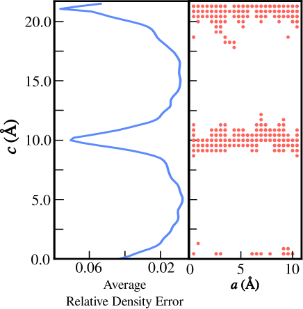
Figure 1: The average relative deviation of the stochastic density from the deterministic density along the c-axis of a silicon supper cell with $128$ atoms ($2\times 2\times 4$) (left panel). The stochastic density was calculated within efsDFT with two non-overlapped $\text{Si}_{64}$ fragments ($2\times 2\times 2$). The right panel shows this relative density difference in projected onto 2D (we only plot deviation above $10\%$). The largest deviations is at the interface between the two fragments ($c\approx 0,10,20\text{\r{A}}$).

The decay of the magnitude of the statistical error with $\sqrt{N_{\chi}}$ implies that in order to reduce the error by an order of magnitude, one has to increase the number of stochastic orbitals by two orders of magnitude. Thus, small statistical errors required to converge local and single particle observables, often require a huge set of stochastic orbitals, making sDFT impractical. Since the standard deviation of the density is proportional to $\rho$$\left(\boldsymbol{r}\right)$ itself (as shown in the supplementary information), the statistical noise can be reduced by decomposing the density into a reference density, $\rho_{\text{ref }}\left(\boldsymbol{r}\right)$, and a correction terms $\Delta\rho\left(\boldsymbol{r}\right)\ll\rho\left(\boldsymbol{r}\right)$, such that $\rho\left(\boldsymbol{r}\right)=\rho_{\text{ref}}\left(\boldsymbol{r}\right)+\Delta\rho\left(\boldsymbol{r}\right)$. This is the central idea behind embedded-fragmented stochastic DFT (efsDFT).(Neuhauser, Baer, and Rabani, 2014; Arnon et al., 2017; Fabian et al., 2018) The system is divided into non-overlapping fragments and the reference density is decomposed as a sum of the fragment densities. This has led to a significant reduction of the noise in efsDFT compared to sDFT when fragments are closed-shell molecules in non-covalently bonded systems.(Neuhauser, Baer, and Rabani, 2014) However, for covalently bonded materials it is necessary to break covalent bonds when fragmenting the system. This leads to an increasingly large statistical error of the density at the boundaries between the fragments (see Fig. 1 for an illustration of this effect for $\text{Si}_{128}$ with PBCs where the system was divided into two non-overlapping $\text{Si}_{64}$ fragments), leading to small improvements of efsDFT with respect to sDFT.(Arnon et al., 2017; Fabian et al., 2018)

III Overlapped Embedded Fragmented stochastic DFT

To overcome the limitation of the efsDFT in covalently bonded fragments, we propose to use overlapping fragments, as sketched in Fig. 2. The basic idea behind the proposed overlapped embedded fragmented stochastic DFT (o-efsDFT) is that each fragment density and density matrix is calculated with a buffer region, but the projection of the fragment density is limited to the core region only. This allows for continuous densities and density matrices across the boundaries between the core fragments, thereby resolving the issue discussed above and allowing for a significant reduction of the statistical error, even for systems with periodic boundary conditions and a delocalized density matrix.

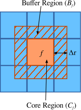
Figure 2: A sketch of the overlapped fragmentation scheme. The system is first divided into non-overlapping core fragments (solid orange and blue regions) of size $C_{f}$ for each fragment $f$. For each core fragment $f$ (orange core), we define a buffer region (dashed red region) of size $B_{f}$. The fragment density is then computed for the core and buffer region together (dressed fragment, $D_{f}$) using periodic boundary condition for $D_{f}$ and projected onto the core, as described in the main text.

As sketched in Fig. 2, the system is divided into non-overlapped fragments that are composed of unit cells and/or small supper cells referred to as “core regions”, labeled $C_{f}$ for fragment $f$. Each core region is then wrapped with a “buffer” region ($B_{f}$) and a dressed fragment (labeled $D_{f}=C_{f}\cup B_{f}$) is defined as the sum of core and buffered regions. For any $\boldsymbol{r}\in C_{f}$, the dressed fragment density matrix ($\langle\boldsymbol{r}|\hat{\rho}_{f}|\boldsymbol{r}^{\prime}\rangle$) is given by:

$$\langle\boldsymbol{r}|\hat{\rho}_{f}|\boldsymbol{r}^{\prime}\rangle=\begin{cases}\sum_{i=1}^{N_{\text{occ}}^{f}}\langle\boldsymbol{r}|\varphi_{i}^{f}\rangle\langle\varphi_{i}^{f}|\boldsymbol{r}^{\prime}\rangle&\boldsymbol{r}^{\prime}\in D_{f}\\ 0&\boldsymbol{r}^{\prime}\not\in D_{f}\end{cases}\;\;\ldotp$$ (6)

In the above equation, $\varphi_{i}^{f}(\boldsymbol{r})$ are KS occupied orbitals for dressed fragment $f$ obtained by a deterministic DFT in region $D_{f}$, where we impose periodic boundary condition for each dressed region separately. The closest distance between the boundaries $C_{f}$ and $D_{f}$ ($\Delta r$, see Fig. 2) is chosen so that periodic boundary conditions can be imposed on region $D_{f}$. Note that the above definition of $\langle\boldsymbol{r}|\hat{\rho}_{f}|\boldsymbol{r}^{\prime}\rangle$ is not necessarily hermitian and idempotent. However, this turns out to be insignificant, since the density matrix of the entire system, remains hermitian regardless of how $\langle\boldsymbol{r}|\hat{\rho}_{f}|\boldsymbol{r}^{\prime}\rangle$ behaves (see more detail below). In the limit were $\Delta r=0$, o-efsDFT is identical to efsDFT.(Neuhauser, Baer, and Rabani, 2014)

With the definition of $\langle\boldsymbol{r}|\hat{\rho}_{f}|\boldsymbol{r}^{\prime}\rangle$ in Eq. (6), the o-efsDFT density at position $\boldsymbol{r}\in C_{f}$ is given by:

$$\rho(\boldsymbol{r}) =\langle\boldsymbol{r}|\hat{\rho}_{f}\hat{\rho}_{f}^{\top}|\boldsymbol{r}\rangle+\langle|\xi(\boldsymbol{r})|^{2}\rangle_{\chi}-\left\langle\langle\boldsymbol{r}|\hat{\rho}_{f}|\chi\rangle\langle\chi|\hat{\rho}_{f}^{\top}|\boldsymbol{r}\rangle\right\rangle_{\chi}$$

$$=\rho_{f}(\boldsymbol{r})+\langle|\xi(\boldsymbol{r})|^{2}\rangle_{\chi}-\langle|\xi^{f}(\boldsymbol{r})|^{2}\rangle_{\chi}\;\;,$$ (7)

where $\xi_{f}(\boldsymbol{r})=\sum_{i=1}^{N_{occ}^{f}}\varphi_{i}^{f}(\boldsymbol{r})\langle\varphi_{i}^{f}|\chi\rangle_{D_{f}}$ and $\langle f|g\rangle_{D_{f}}=\int_{D_{f}}\mathrm{d}\boldsymbol{r}f^{\ast}(\boldsymbol{r})g(\boldsymbol{r})$, i.e. integration over the dressed fragment region. It is easy to verify that the density in Eq. (7) satisfies the following requirements:

1. In the infinite sampling limit the properties calculated from o-efsDFT converge to deterministic DFT results.

2. If $C_{f}$ is the system itself, properties calculated from o-efsDFT are equal to those from the deterministic DFT calculation regardless of the number of stochastic orbitals.

3. Given any partitioning of the system into core regions, in the limit where the buffered zone grows such that $D_{f}$ represents the entire system, properties calculated from o-efsDFT will, again be equivalent to the deterministic results with any number of stochastic orbitals.

We now turn to discuss the calculations of kinetic energy, the nonlocal pseudopotential energy, and the nonlocal force using the above formalism with overlapped fragments. The calculation of the local pseudopotential energy, the Hartree term, the exchange correlation energies, and the corresponding forces can be obtained directly using the density in Eq. (7), similar to sDFT (Baer, Neuhauser, and Rabani, 2013) and efsDFT.(Neuhauser, Baer, and Rabani, 2014; Arnon et al., 2017) The kinetic energy is evaluated in real-space by integrating the kinetic energy density over the core region of each fragment:

$$E_{K} =\sum_{f}\sum_{i=1}^{N_{occ}^{f}}\langle\varphi_{i}^{f}|\hat{t}|\varphi_{i}^{f}\rangle_{C_{f}}$$

$$+ \left\langle\langle\xi|\hat{t}|\xi\rangle\right\rangle_{\chi}-\sum_{f}\left\langle\langle\xi_{f}|\hat{t}|\xi_{f}\rangle_{C_{f}}\right\rangle_{\chi}.$$ (8)

For an infinite sample set ($N_{\chi}\rightarrow\infty$), $\left\langle\langle\chi|\varphi_{i}^{f}\rangle_{D_{f}}\langle\varphi_{j}^{f}|\chi\rangle_{D_{f}}\right\rangle_{\chi}=\langle\varphi_{j}^{f}|\varphi_{i}^{f}\rangle_{D_{f}}=\delta_{ij}$. Therefore, the first and third terms in Eq. (8) cancel each other. Similarly, the non-local pseudopotential energy ($E_{\text{nl}}$) can be calculated as follows:

$$E_{\text{nl}} =\sum_{f}\sum_{\text{atom}\in C_{f}}\sum_{i=1}^{N_{occ}^{f}}\langle\varphi_{i}^{f}|\hat{v}_{\text{nl}}^{\text{atom}}|\varphi_{i}^{f}\rangle_{D_{f}}+\left\langle\langle\xi|\hat{v}_{nl}|\xi\rangle\right\rangle_{\chi}$$

$$- \sum_{f}\sum_{\text{atom}\in C_{f}}\left\langle\langle\xi_{f}|\hat{v}_{\text{nl}}^{\text{atom}}|\xi_{f}\rangle_{D_{f}}\right\rangle_{\chi},$$ (9)

where $\hat{v}_{\text{nl}}^{\text{atom}}$ is the non-local pseudopotential operator for each atom and the sum $\sum_{\text{atom}\in C_{f}}$ refers to summation over all atoms that are in region $C_{f}$. The non-local pseudopotential nuclear force for each atom with a position $R_{\text{atom}}\in C_{f}$, is given by:

$$\boldsymbol{F}_{\text{nl}}^{\text{atom}} =\sum_{i=1}^{N_{occ}^{f}}\left\langle\varphi_{i}^{f}\left|\frac{\partial\hat{v}_{nl}^{\text{atom}}}{\partial\boldsymbol{R}_{\text{atom}}}\right|\varphi_{i}^{f}\right\rangle_{D_{f}}$$

$$+ \left\langle\left\langle\xi\left|\frac{\partial\hat{v}_{nl}^{\text{atom}}}{\partial\boldsymbol{R}_{\text{atom}}}\right|\xi\right\rangle\right\rangle_{\chi}-\left\langle\left\langle\xi_{f}\left|\frac{\partial\hat{v}_{nl}^{\text{atom}}}{\partial\boldsymbol{R}_{\text{atom}}}\right|\xi_{f}\right\rangle_{D_{f}}\right\rangle_{\chi}.$$ (10)

It is straightforward to show that Eqs. (9) and (10) satisfy all three requirements above.

IV Implementation

System	Fragment	$N_{\chi}$	$E_{K}/N_{e}$	$E_{\text{nl}}/N_{e}$	$E_{\text{loc}}/N_{e}$	$E_{\text{tot}}/N_{e}$
Si512	Deterministic		10.3577	6.1274	-8.6267	-26.9954
	Si8	800	10.3596(88)	6.1269(29)	-8.6215(41)	-26.9881(77)
	Si64	80	10.3523(21)	6.1277(59)	-8.6223(61)	-26.9955(12)
	Si216	80	10.3560(13)	6.1284(15)	-8.6265(27)	-26.9959(5)
Si1728	Si64	80	10.3507(14)	6.1287(25)	-8.6207(31)	-26.9953(11)
	Si216	80	10.3527(5)	6.1286(7)	-8.6227(6)	-26.9964(2)
Si4096	Si64	80	10.3526(23)	6.1286(5)	-8.6219(13)	-26.9944(12)
	Si216	80	10.3539(7)	6.1296(7)	-8.6243(11)	-26.9957(5)

Table 1: Si₅₁₂, Si₁₇₂₈, Si₄₀₉₆ were calculated by o-efsDFT with Si₆₄/Si₂₁₆ as fragments. Kinetic energy per electron, non-local pseudo-potential energy per electron, and total energy per electron (in eV) are presented in the table. The standard deviation in the last digits of energies are listed in parenthesis. Deterministic DFT calculation of Si₅₁₂ is also presented.

The o-efsDFT approach can be implemented for any planewave or real-space based approach. The necessary steps to complete the self-consistent iteration to converge the density, energy and forces, can be summarized as follows (for a planewave based approach):

1. Perform a deterministic DFT calculation in region $D_{f}$ for each fragment $f$ using a real-space grid spacing that equals that the grid spacing of the full system.

2. Using the fragment density as an initial guess, generate the corresponding Kohn-Sham potential.

3. Generate a set of stochastic orbitals $|\chi_{1}\rangle\cdots|\chi_{N_{\chi}}\rangle$ on a real-space grid and then transform to reciprocal space (it requires $\approx N_{g}/2$ grid points in reciprocal space to store an $N_{g}$ real-space orbital due to the isotropic kinetic energy cutoff).

4. For all stochastic orbital $|\chi\rangle$, expand the action of the density matrix in terms of Chebyshev polynomials and tune the chemical potential to satisfy:

   $$N_{e}(\mu) +\sum_{f}\int_{C_{f}}\mathrm{d}\boldsymbol{r}\rho^{f}(\boldsymbol{r})$$

   $$- \sum_{f}\int_{C_{f}}\mathrm{d}\boldsymbol{r}\langle|\xi_{f}(\boldsymbol{r})|^{2}\rangle_{\chi}=N_{e}\,\,,$$ (11)

   where as before, $N_{e}(\mu)=\left\langle\left\langle\chi\left|\theta_{\beta}(\mu-\hat{h}_{\text{KS}})\right|\chi\right\rangle\right\rangle_{\chi}$, $\rho_{f}(\boldsymbol{r})$ is define in Eq. (7), $\xi_{f}\left(\boldsymbol{r}\right)=\sum_{i=1}^{N_{occ}^{f}}\varphi_{i}^{f}(\boldsymbol{r})\langle\varphi_{i}^{f}|\chi\rangle_{D_{f}}$, and $N_{e}$ is the number of electrons in the system.

5. Use the chosen $\mu$ from the previous step to generate a set of stochastic project orbitals, $|\xi\rangle=\sqrt{\theta_{\beta}(\mu-\hat{h}_{\text{KS}})}|\chi\rangle$, using a Chebyshev or Newton interpolation polynomials to act with $\sqrt{\theta_{\beta}(\mu-\hat{h}_{\text{KS}})}$ on $|\chi\rangle$.

6. Calculate the density $\rho(\boldsymbol{r})$ using Eq. (7) and the corresponding energy with Eqs. (8) and (9). The other energy terms can be obtained directly from the density, similarly to the deterministic DFT.

7. Use the density as input for the next iteration and go to step (d). Repeat until converges is achieved.

Throughout the self-consistent iterations the same random number seed was used to generate the stochastic orbitals. This is necessary to converge the self-consistent procedure to a tolerance similar to deterministic DFT. This also reduces the computational effort associated with projecting the stochastic orbitals onto the fragments, so that the first and last terms in Eqs. (7) – (10) were calculated prior to the self-consistent loop.

V Results and Discussion

To assess the accuracy of the o-efsDFT method and its limitations, we performed $\Gamma$ point calculations on a set of silicon crystals with varying super-cell size. Bulk silicon is rather challenging for linear scaling DFT due to its particularly small LDA band gap.(Skylaris and Haynes, 2007) A grid spacing of 0.41$a_{0}$ corresponding to a planewave cutoff of $60$ Ryd was used to converge the energy and force to within an acceptable tolerance. To reduce the energy range of the KS-Hamiltonian, we used an “early truncation” scheme for the kinetic energy operator in which the magnitude of the reciprocal space vector $\boldsymbol{k}$ (used in evaluating the kinetic energy operator acting on a wave function) was replaced by $\min\{\|\boldsymbol{k}\|,k_{\text{ke}}\}$, where $k_{\text{ke}}=\sqrt{2E_{\text{cut}}^{\text{ke}}}$, with $E_{\text{cut}}^{\text{ke}}=20$ Ryd for all $3$ systems studied here. The Troullier-Martins norm conserving pseudopotentials (Troullier and Martins, 1991) were used together with the Kleinman-Bylander separable form.(Kleinman and Bylander, 1982) The pseudopotentials were evaluated in real-space to reduce the computational scaling.(King-Smith, Payne, and Lin, 1991) In the Fermi function $\beta$ was set to $\approx 600$ inverse Hartree, which is sufficient to converge the ground state properties to within an error much smaller than the statistical error.

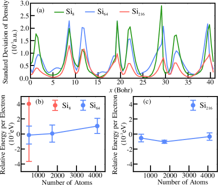
Figure 3: Panel (a): The standard deviation of the density along the $x$-axis for $y=z=0$ for $\text{Si}_{512}$ with three different dressed fragment sizes (all for $\text{Si}_{8}$ core fragment), as specified in the legend. Panels (b) and (c): The energy per electron (relative to that of a deterministic DFT calculation for $\text{Si}_{512}$) as a function of the system size for dressed fragment of $\text{Si}_{64}$(panel (b)) and $\text{Si}_{216}$ (panel (c)) with $N_{\chi}=80$. In panel (b) we also show the result with $\text{Si}_{8}$ dressed fragment (namely, no overlap between the fragments) with $N_{\chi}=800$, where we also observe a large bias (Fabian et al., 2018) and find that the energy is larger by $4$ eV per atom compared to the deterministic value.

We studied bulk silicon with $3$ supper cells of size $4\times 4\times 4$ unit cells ($N_{\text{atom}}=512$), $6\times 6\times 6$ unit cells ($N_{\text{atom}}=1728$), and $8\times 8\times 8$ unit cells ($N_{\text{atom}}=4096$). Core fragments of $\text{Si}_{8}$were used to partition all systems while three different buffer regions were adopted for forming the dressed fragments with $8$, $64$, and $216$ Si atoms. $N_{\chi}=80$ stochastic orbitals were used in each calculation but for the non-overlapped Si₈ fragments, we used $N_{\chi}=800$ stochastic orbitals. It should be noted that calculations with $N_{\chi}=80$ stochastic orbitals failed to converge without using overlapped fragments. The self-consistent iteration were converged using DIIS (Pulay, 1980, 1982; Kresse and Furthmuller, 1996) with a convergence criteria set to $10^{-8}$ Hartree per electron.

Table 1 summarizes the results for the kinetic, nonlocal, local, and total energies per electron for all three system sizes studied and for all dressed fragments used. The external local potential energy per electron, $E_{\text{loc}}/N_{e}$, depends linearly on the density and provides a reliable measure of the accuracy of the stochastic density. As can be seen in Table 1, for Si₅₁₂, $E_{\text{loc}}/N_{e}$ with dressed fragments of sizes Si₆₄ and Si₂₁₆ the external potential energy per electron agrees well with the deterministic DFT result, where the differences between the two are well within the error bars of $5$ independent o-efsDFT runs. Reductions in the standard deviation of $E_{\text{loc}}/N_{e}$ with respect to the dressed fragment size was observed in all $3$ system sizes.

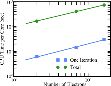
Figure 4: A log-log plot of the CPU time per core versus the number of electrons. The green and blue symbols are for the total wall time of all self-consistent iterations and for a single self-consistent iteration, respectively. The straight lines are fits to a power law with exponents of $N_{e}^{0.71}$ and $N_{e}^{0.77}$, respectively.

This is also illustrated in panel (a) of Fig. 3, where we plot the density along the $x$-axis (at fixed $y$ and $z$) for Si₅₁₂ for all three dressed fragment sizes. The non-overlapping fragments required $10$ times more stochastic orbitals ($N_{\chi}=800$) in order to reduce the noise in the density to similar levels as the overlapping Si₆₄ dressed fragments. For Si₂₁₆ dressed fragments, the noise in the density dropped by a factor of $\approx 2$, suggesting that only $N_{\chi}=20$ stochastic orbitals are needed to converge the density to the same level of noise as that of Si₆₄ dressed fragments.

The decrease in the noise with increasing buffer sizes (increase $B_{f}$ region) is not limited to the density itself or to local observables that depends directly on the density, like $E_{\text{loc}}/N_{e}$. The kinetic energy per electron ($E_{K}/N_{e}$) and non-local pseudopotential energy per electron ($E_{\text{nl}}/N_{e}$) also show a significant reduction in their variance with increasing $B_{f}$, as can be seen in Table 1. Comparing to the deterministic results for Si₅₁₂ we find that o-efsDFT provides energies per electron that are within $10^{-3}$ eV from the deterministic values and that the agreement improves with the size of the buffer regions. This is also illustrated in panels (b) and (c) of Fig. 3, where we plot the total energy per electron (relative to a reference energy of the deterministic result for Si₅₁₂) for the $3$ system sizes and for $3$ different buffer regions (Si₈,Si₆₄, and Si₂₁₆) studied in this work. As before, we use $N_{\chi}=80$ stochastic orbitals except for $\text{Si}_{8}$ buffer region, where $N_{\chi}=800$. The total energy per electron contains much larger noise when the fragments do not overlap, even when the number of stochastic orbitals was $10$ larger. Replacing the Si₈ fragment with a dressed Si₆₄ fragment significantly reduces the noise in the total energy per electron and further reduction in the noise was achieved by enlarging the buffer region, i.e. using Si₂₁₆ as dressed fragment.

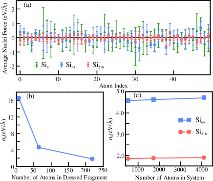
Figure 5: Panel (a): Nuclei forces along $x$-axis for $50$ representative atoms in Si₅₁₂ with Si₆₄ (blue) and Si₂₁₆ (red) dressed fragments and for $N_{\chi}=80$. The dots and error bars are averages and standard deviations of the forces from $5$ independent runs. Panel (b) and (c) show the value of $\sigma_{0}$ (see the main text for definition) as a function of the buffer size and the number of electrons, respectively.

Within the accuracy of the current calculations, we find that the statistical error in the total energy per electron is similar for all $3$ system sizes studied here (for a fixed buffer size), implying that self-averaging is not significant.(Baer, Neuhauser, and Rabani, 2013) This suggests that o-efsDFT scales nearly linearly with the system size, as indeed is observed for the scaling of the energy per electron, shown in Fig. 4. We focused on the computational cost of the self-consistent iterations which dominates the overall CPU time. Since parallelism over stochastic orbitals is straightforward and the communication time is negligible, we report the CPU time per stochastic orbital (each orbital was distributed on a different node). Our results show that the time used in each self-consistent scales as $O\left(N_{e}^{0.77}\right)$. The net CPU time per stochastic orbital over all self-consistent iterations scales as $O\left(N_{e}^{0.71}\right)$, which suggests that the number of self-consistent iterations does not significantly increases with increasing system size. We note that the practical scaling is somewhat better than linear ($O\left(N_{e}\right)$) mainly due to improved multithreading timings for larger grids. This however, may depend on the computational architecture used and on the range of systems studied. Generally, we expect the approach to scale as $O\left(N_{e}\right)$ for large systems.

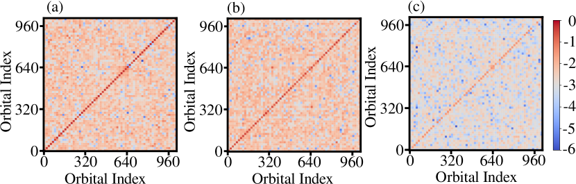
Figure 6: Fragment density matrices difference $\Delta\hat{\rho}=\sum_{{}_{f}}\hat{\rho}_{f}-\hat{\rho}$ evaluated for Si₅₁₂ with (a) non-overlapped Si₈ fragment, (b) non-overlapped Si₆₄ fragment, and (c) overlapped Si₆₄ fragments. Fragment density matrices are represented in the subspace spanned by occupied orbitals of Si₅₁₂ In this representation, the system density matrix $\hat{\rho}$ becomes the identity matrix. To span several orders of magnitude in the values $\Delta\hat{\rho}$ we use a logarithmic color scale.

In addition to computing the individual contribution to the total energy per electron, o-efsDFT also offers an efficient and accurate approach to compute the forces on each atom. Panel (a) of Fig. 5 shows the average and standard deviation of nuclear forces from $5$ independent o-efsDFT runs for $50$ representative atoms in Si₅₁₂. The forces are computed for the equilibrium structure and thus should fluctuate about $0$. Forces from o-efsDFT with non-overlapped fragment and $N_{\chi}=800$ stochastic orbitals fluctuate with comparable standard deviations as those from o-efsDFT with Si₆₄ dressed fragments and $N_{\chi}=80$ stochastic orbitals, yet the computational effort is nearly $10$ times smaller in the latter. Smaller force fluctuations were observed with growing buffer region, similar to the reduction in the statistical noise in the total energy per electron.

A summary of the statistical error in the forces as a function of the size if the dressed fragment and as a function of the system size are shown in panels (b) and (c) of Fig. 5, respectively. Within the central limit theorem, we assume that the standard deviation of nuclei force decays as $\sigma_{0}/\sqrt{N_{\chi}}$ where $\sigma_{0}$ is the standard deviation with only $1$ stochastic orbital. In panel (b) we plot $\sigma_{0}$ as a function of the dressed fragment size, where a significant reduction is clearly observed. Panel (c) shows that $\sigma_{0}$ does not change significantly with system size, suggesting that the number of stochastic orbitals does not increase with the system size for a given statistical error, suggesting that the scaling for the force follows that of the energy per electron shown in Fig. 4.

VI Overlapped versus Non-overlapped Fragments

To further understand the o-efsDFT results presented in the previous section we examine the role played by the overlap of fragments. In the supplementary information we derive an expression for the variance of the density in terms of the density itself and the density matrix:

$$\text{Var}\left\{\rho\left(r\right)\right\} \leq\left(2\max_{\boldsymbol{r}^{\prime}}\langle\boldsymbol{r}^{\prime}|2\hat{\rho}+\Delta\hat{\rho}^{\top}|\boldsymbol{r}\rangle^{2}+4\rho(\boldsymbol{r})\right)$$

$$\times \int\mathrm{d}\boldsymbol{r}^{\prime}\langle\boldsymbol{r}|\Delta\hat{\rho}|\boldsymbol{r}^{\prime}\rangle^{2}$$ (12)

where $\Delta\hat{\rho}=\sum_{f}\hat{\rho}_{f}-\hat{\rho}$ and $\hat{\rho}_{f}$ and $\rho$ are defined in Eq. (6) and above Eq. (1), respectively. It is clear that the noise in the density is not just correlated with the density, but also with the density matrix. Thus, fragmentation schemes to reduce the noise in $\rho\left(\boldsymbol{r}\right)$ must provide a reasonable approximation for the density matrix across different fragments. This is not the case for the non-overlap fragments, where off-diagonal matrix elements of the full reference density matrix ($\sum_{f}\hat{\rho}_{f}$) for different fragments vanish, leading to a significant level of noise. In o-efsDFT with non-vanishing buffer zones, the reference density matrix is allowed to decay at least within distance $\Delta r$ before it is truncated to $0$ (see Fig. (2)). This improves the reference density matrix and the resulting noise is significantly reduced as the size of the buffer zone increases.

In Fig. 6 we show the reference density matrix for three different fragmentation schemes. Panels (a) and (b) correspond to non-overlapped fragments with $\text{Si}_{8}$ and $\text{Si}_{64}$ fragments, respectively and panel (c) shows the reference density matrix for $\text{Si}_{8}$ with a dressed fragment of $\text{Si}_{64}$. In the eigenfunction representation, the density matrix should equal the identity matrix. This is clearly not the case for panel (a) and (b), but is rather close to the unit matrix for panel (c). This is rather surprising since even with fragments that equal the size of the the dressed fragment, the density matrix does not improve. Obviously, the discontinuity in the density matrix at the interfaces between fragments does not depends on the size of the fragment for the non-overlapped case, leading to significant noise in the density even for large fragments. While it only takes a small fragment, $\text{Si}_{8}$, with a buffer zone of $\text{Si}_{64}$ to significantly reduce the noise.

VII Conclusion

Motivated by the need to reduce significantly the noise level in linear scaling sDFT, we have proposed a new fragmentation scheme that circumvents some of limitations of our original embedded-fragmented stochastic DFT approach, mainly for covalently bonded systems. While previous attempts to develop a fragmentation scheme were based solely on providing a good reference system for the density alone, here, we showed that this is not a sufficient criteria. Based on detailed analysis of the variance in the density, we developed a new overlapped fragmentation scheme, which provides an excellent reference for both the density matrix and the density. By dividing the system into non-overlapped core fragments and overlapped dressed fragments, we demonstrated that the existence of a buffer zone is crucial in the reduction of the stochastic noise in the energy per electron and nuclear forces. Moreover, we showed that the stochastic noise does not increase with respect to system size when using a fixed fragment sizes nor does the number of self-consistent iterations, leading to a practical scaling that is slightly better than the expected linear scaling. While all application in this study were limited to bulk silicon with periodic boundary condition, we wish to iterate that the approach is also valid for open boundary conditions, were we expect it to work equally well.