Randomization Tests for Equality in Dependence Structure

Abstract

We develop a new statistical procedure to test whether the dependence structure is identical between two groups. Rather than relying on a single index such as Pearson’s correlation coefficient or Kendall’s $\tau$, we consider the entire dependence structure by investigating the dependence functions (copulas). The critical values are obtained by a modified randomization procedure designed to exploit asymptotic group invariance conditions. Implementation of the test is intuitive and simple, and does not require any specification of a tuning parameter or weight function. At the same time, the test exhibits excellent finite sample performance, with the null rejection rates almost equal to the nominal level even when the sample size is extremely small. Two empirical applications concerning the dependence between income and consumption, and the Brexit effect on European financial market integration are provided.

Keywords: copula; randomization test; permutation test

1 Introduction

As the most fundamental measure of dependence, Pearson’s coefficient of correlation has been widely used for centuries in numerous empirical studies concerning the dependence between variables. Despite its lasting popularity, however, Pearson’s coefficient of correlation certainly has some limitations in characterizing dependence structures because it only captures pairwise and linear dependence. When the variables of interest are Gaussian where the linearity is implied, the correlation coefficient serves as the best measure of dependence in the sense that the dependence structure is fully described by the correlation. Nevertheless, it is not always reasonable to presume that the underlying dependence structure is linear and in fact, many economic and financial data frequently exhibit nonlinear relationships.

Alternatively, we may aim to provide a meaningful description of the entire dependence structure rather than summarize it using a single index, particularly if nonlinear features of the variables such as asymmetric dependence or tail dependence are of interest. In this context, dependence functions, also known as copulas, have proved to be useful in the studies of dependence structures. Suppose that $X_{1},...,X_{d}$ are random variables with joint distribution function $H$ and univariate margins $F_{1},...,F_{d}$. Sklar’s theorem (1959) ensures the existence of a joint distribution function $C:[0,1]^{d}\rightarrow[0,1]$ that has uniform margins and satisfies

$$H(x_{1},...,x_{d})=C(F_{1}(x_{1}),...,F_{d}(x_{d}))$$ (1)

for all $(x_{1},...,x_{d})\in\mathbb{R}^{d}$. The function $C$ is called the copula associated with $H$. This result suggests that any joint distribution can be decomposed into two parts, the univariate marginal distributions which determine the behavior of individual variables, and the copula function which determines the dependence structure between variables. For the reason, copulas have been major concerns in various applications of dependence modelling.

In this paper, we use the copulas to propose a statistical procedure for testing homogeneity of dependence structure between different groups. By comparing copulas, our test detects any arbitrary form of dissimilarity in the dependence structure. The test statistic is constructed based on the $L_{p}$ distance between two empirical copulas and critical values are obtained from a novel randomization procedure. Implementation of our test is intuitive and straightforward, and does not require any specification of a tuning parameter or weight function that can be arbitrarily chosen by a researcher. At the same time, the test exhibits substantially excellent performance in finite samples, with the null rejection rates almost equal to the nominal level even when the sample size is extremely small.

In developing our methodology, we adapt the permutation method used to test distributional equality. A modification is required because the null set of copula equality is strictly larger than the null set of distributional equality. When the problem is to test the equality of distributions, classical permutation tests deliver exact size control and those tests are as powerful as standard parametric tests under general conditions (Hoeffding, 1952). However, when the null hypothesis to be tested is larger than distributional equality, the usual permutation tests generally do not control size even when the sample size is large (Romano, 1990; Chung and Romano, 2013). Therefore, we expect that a naive application of a permutation test to the hypothesis of copula equality may fail to deliver valid inference even asymptotically.

To resolve this problem, recent studies on randomization tests focus on the studentization of a test statistic. See, for instance, Neuhaus (1993), Janssen (1997, 1999, 2005), Janssen and Pauls (2003, 2005), Neubert and Brunner (2007), Omelka and Pauly (2012) and Chung and Romano (2016). These modifications provide asymptotic level $\alpha$ tests of relevant null hypotheses, with exact size control under distributional equality. However, this approach is not applicable in our context because our test statistic has more or less complicated form and its sampling distribution involves several Brownian bridges determined by underlying copulas, and the derivatives of those copulas. Henceforth, we take a different approach introducing theorems of conditional convergence in the context of randomization test literature. Although we only focus on the copula equality, our technical ingredients may be useful for handling other null hypotheses where the test statistic is not linear and the delta method is to be invoked.

The remainder of the paper is structured as follows. In Section 2, we explain why the classical permutation method is invalid when used to test copula equality. Our main results are presented in Section 3, where we introduce modified randomization procedures and discuss their asymptotic properties. In Section 4, we report some numerical simulation results. In Section 5, two empirical applications concerning the dependence between income and consumption, and the Brexit effect on European financial market integration are provided. Proofs of lemmas and theorems are collected together in the Appendix.

2 Application of the permutation method

Suppose that $X^{1},...,X^{n}$ are i.i.d. draws from a distribution $H_{1}\,$and $Y^{1},...,Y^{m}$ are i.i.d. draws from a distribution $H_{2}$. The two samples are independent. Each distribution is $d$-variate with $d\in\mathbb{N}$, and we write $X^{i}=(X_{1}^{i},\ldots,X_{d}^{i})$ and $Y^{j}=(Y_{1}^{j},\ldots,Y_{d}^{j})$ for $i=1,...,n$ and $j=1,...,m$. We denote the univariate margins of $H_{1}$ by $F_{1},\ldots,F_{d}$ and the univariate margins of $H_{2}$ by $G_{1},\ldots,G_{d}$. Let $N$ be the total number of observations (that is, $N=n+m$), and let $W$ be the stacked matrix of the size $N\times d$,

$$W=(W^{1};W^{2};...;W^{N})=(X^{1};...;X^{n};Y^{1};...;Y^{m})\text{. }$$ (2)

For the case of testing the hypothesis $\mathcal{H}_{0}:(H_{1},H_{2})\in\Theta_{00}$ with $\Theta_{00}=\{(H,H^{\prime})\in\mathbb{D}^{2}|H=H^{\prime}\}$, where $\mathbb{D}$ is the set of all $d$-variate probability distributions, we may easily construct an exact level $\alpha$ test using a randomization test based on permuting the rows of $W$. Complications arise when the null hypothesis of interest is strictly larger than $\Theta_{00}$. If this is the case, it is well known that permutation tests generally cannot control the probability of Type I error even asymptotically. Hence, inferences based on a permutation test can be highly misleading (Romano, 1990; Chung and Romano, 2013).

Let $\Phi:\mathbb{D}\rightarrow\ell^{\infty}([0,1]^{d})$ be the map that sends a cdf $\tilde{H}\in\mathbb{D}$ with margins $\tilde{F}_{1},...,\tilde{F}_{d}$ to $\tilde{H}(\tilde{F}_{1}^{-1},...,\tilde{F}_{d}^{-1})$. For each $k=1,...,d$ and $t\in[0,1]$, $\tilde{F}_{k}^{-1}(t)$ is defined to be $\inf\{x|\tilde{F}_{k}(x)\geq t\}$. In words, given a joint distribution function, $\Phi$ is the map which provides the corresponding copula as an output. Now we can formulate our null hypothesis of copula equality as

$$\mathcal{H}_{0}:(H_{1},H_{2})\in\Theta_{0}\text{ with }\Theta_{0}=\{(H,H^{\prime})\in\mathbb{D}^{2}|\Phi(H)=\Phi(H^{\prime})\}\text{.}$$ (3)

Since we may have two different distributions $H_{1}$ and $H_{2}$ which share the same copula, our null set $\Theta_{0}$ is strictly larger than $\Theta_{00}$. This implies that a randomization test based on the permutations of $W$ may possibly lead to a permutation distribution which does not agree with the correct limit of our test statistic.

To illustrate this point, let’s consider the following example with two bivariate ($d=2$) cdfs $H_{1}$ and $H_{2}$. We let $H_{1}$ be the distribution of $X_{1}$ and $X_{2}$ where $X_{1}$ is uniformly distributed between zero and one, and $X_{2}$ is defined to be $X_{1}+1$. Now consider another distribution $H_{2}$, that is the distribution of $Y_{1}$ and $Y_{2}$, where $Y_{2}$ is uniformly distributed between zero and one, and $Y_{1}$ is defined to be $Y_{2}+1$. The joint distributions $H_{1}$ and $H_{2}$ are given by $H_{1}(x_{1},x_{2})=\min(x_{1},x_{2}-1)$ on $(x_{1},x_{2})\in[0,1]\times[1,2]$ and $H_{2}(x_{1},x_{2})=$ $\min(x_{1}-1,x_{2})$ on $(x_{1},x_{2})\in[1,2]\times[0,1]$, respectively. See Figure 2.1 for a graphical illustration of the shapes of the distributions. For both $H_{1}$ and $H_{2}$, it is easy to verify that the associated copula is $C_{1}(u_{1},u_{2})=C_{2}(u_{1},u_{2})=\min(u_{1},u_{2})$ for $(u_{1},u_{2})\in[0,1]^{2}$. We see that $H_{1}$ and $H_{2}$ are different but their copulas $C_{1}$ and $C_{2}$ are identical. In other words, $(H_{1},H_{2})\in\Theta_{0}$ but $(H_{1},H_{2})\notin\Theta_{00}$.

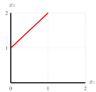
(a)

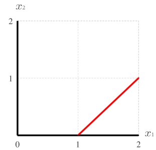
(b)

Figure 1: In our example, $X_{1}$ and $X_{2}$ with the joint distribution $H_{1}$ are distributed evenly over the the bold line displayed in Panel (a) while $Y_{1}$ and $Y_{2}$ with the joint distribution $H_{2}$ are distributed evenly over the bold line displayed in Panel (b).

Suppose we will use a test statistic $T_{n,m}$ to test copula equality. The limit distribution of $T_{n,m}$ may generally depend on the underlying copulas and we hope to approximate it using the permutation distribution of $T_{n,m}$. Since the permuted samples behave as though drawn from a mixture of $H_{1}$ and $H_{2}$, the permutation distribution of $T_{n,m}$ can be inferred from its unconditional distribution when the samples are drawn from that mixture distribution. This argument is well explained in Chung and Romano (2013), where the authors employed a contiguity argument and coupling construction assuming the linearity of $T_{n,m}$. Although our test statistic in the next section is not linear with respect to the original sample, the validity of our test procedure can be demonstrated by applying results in Chung and Romano (2013) to a simpler infeasible test statistic whose construction depends on the univariate margins being known. Viewing our test in this light, it is natural to ask how the copula of a mixture of $H_{1}$ and $H_{2}$ is determined.

Now return to our example and consider a mixture of $H_{1}$ and $H_{2}$ defined by $\bar{H}=\lambda H_{1}+(1-\lambda)H_{2}$ with some weight $\lambda\in[0,1]$. The support of the mixture distribution $\bar{H}$ is displayed in Panel (a) of Figure 2.2. When $\lambda=1/2$ for instance, $\bar{H}$ corresponds to the distribution of a pair of random variables uniformly distributed over the two diagonals in Panel (a) of Figure 2.2. The corresponding copula in this case is,

$$C^{\dagger}(u_{1},u_{2})=\begin{array}[]{c}\begin{cases}\min(u_{1},u_{2}-\frac{1}{2})\text{ \ \ \ \ for }(u_{1},u_{2})\in\left[0,\frac{1}{2}\right]\times\left[\frac{1}{2},1\right]\\ \min(u_{1}-\frac{1}{2},u_{2})\text{ \ \ \ \ for }(u_{1},u_{2})\in\left[\frac{1}{2},1\right]\times\left[0,\frac{1}{2}\right]\\ \max(u_{1}+u_{2}-1,0)\text{ \ \ \ \ \ \ otherwise,}\end{cases}\end{array}$$

which has the uniform probability mass over the bold lines in Panel (b) of Figure 2.2. We observe from this example that the copula associated with the mixture distribution $\bar{H}$ can be different from $C_{1}$ (or $C_{2}$) even when $C_{1}=C_{2}$.

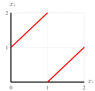
(a)

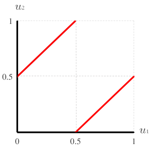
(b)

Figure 2: Panel (a) displays the support of $\bar{H}$ in our example. When $\lambda=1/2$, $\bar{H}$ is the distribution of a pair of random variables uniformly distributed over the two diagonals. Panel (b) describes the corresponding copula associated with $\bar{H}$ when $\lambda=1/2$.

The discussion in the preceding paragraph should provide some insight into why a permutation test obtained by permuting the rows of $W$ can be invalid. Failure of such a permutation test may be attributed to the fact that (i) the limit distribution of $T_{n,m}$ is determined by the true underlying copulas in general, and (ii) unless $\lambda$ is zero or one, the copula of the mixture distribution is different from $C_{1}$ or $C_{2}$. In our example above, the limit of $T_{n,m}$ is determined by $C_{1}$ which is equal to $C_{2}$, whereas the limit of the permutation distribution is determined by the copula associated with the mixture distribution with $\lambda$ being determined by the limiting value of $n/(n+m)$. This suggests that estimating the asymptotic null distribution of $T_{n,m}$ by permuting the samples from $H_{1}$ and $H_{2}$ may not be adequate.

A natural solution to this problem is to manipulate the test statistic in such a way that its limiting distribution does not depend on the underlying probability distributions or copulas. When applied to a properly studentized test statistic, a permutation test can deliver asymptotically valid inference in the sense that the rejection probability converges to the nominal level $\alpha$ when the null hypothesis is true. However, this can only be done in limited circumstances where the test statistic is of a simple linear form. For more general applications of the permutation method, it requires more technical development.

To adapt the permutation method for the inference of copula equality, we will instead commence from the observation that copulas can be regarded as the joint distribution of the probability integral transform of each univariate variable. For instance, the copula in (1) is the joint distribution of $d$ random variables, $F_{1}(X_{1}),...,F_{d}(X_{d})$. From this point of view, the problem of testing copula equality is closely related to the problem of testing the equality of probability distributions; assuming that the univariate margins $F_{1},...,F_{d}$ are known, the classical theory of randomization tests applies and an exact $\alpha$ level test can be constructed by the permutation method. However, the marginal distributions are not known in practice and can only be estimated consistently, and this suggests that we may only rely on asymptotic group invariance conditions in our application of the permutation method. In this respect, our results in the next section complement those of Canay et al. (2017) or Beare and Seo (2017), who investigated the behavior of randomization tests under approximate symmetry conditions, albeit with different formalizations of approximate symmetry.

3 Test construction

In this section, we explain how to construct valid permutation tests of the hypothesis of equal dependence structure. Two asymptotically valid procedures are proposed. The first is similar to the multiplier technique of Rémilard and Scaillet (2009). The second is a modification of the first that eliminates the need for partial derivative estimation. Our main results are summarized in Theorem 3.1 and Theorem 3.2. Although we confine our attention to the two-sample problem for simplicity, it is straightforward to extend our results to the more general $k$-sample problem.

We start out by defining the test statistic. As in the previous section, let $C_{1}$ and $C_{2}$ be the copulas associated with $H_{1}\,$and $H_{2}$ respectively; that is, $C_{1}=\Phi(H_{1})$ and $C_{2}=\Phi(H_{2})$. Since our null hypothesis is given as in (3), a proper test statistic can be constructed based on the discrepancy between $C_{1}$ and $C_{2}$. Let $\hat{F}_{1,n},...,\hat{F}_{d,n},\hat{G}_{1,m},..,\hat{G}_{d,m}$ be the empirical distributions corresponding to $F_{1},...,F_{d}$, $G_{1},...,G_{d}$,

$$\hat{F}_{q,n}(x)=\frac{1}{n}\sum_{i=1}^{n}1(X_{q}^{i}\leq x),\quad\hat{G}_{q,m}(x)=\frac{1}{m}\sum_{j=1}^{m}1(Y_{q}^{j}\leq x)\text{ for }q=1,...,d\text{ and }x\in\mathbb{R}\text{, \ }$$ (4)

and $\hat{C}_{1,n}$, $\hat{C}_{2,m}$ be the empirical copulas computed from the two independent samples as below.

$$\hat{C}_{1,n}(u_{1},...u_{d}) = \frac{1}{n}\sum_{i=1}^{n}1\{\hat{F}_{1,n}(X_{1}^{i})\leq u_{1},...,\hat{F}_{d,n}(X_{d}^{i})\leq u_{d}\}\text{ and}$$

$$\hat{C}_{2,m}(u_{1},...u_{d}) = \frac{1}{m}\sum_{i=1}^{m}1\{\hat{G}_{1,m}(Y_{1}^{j})\leq u_{1},...,\hat{G}_{d,m}(Y_{d}^{j})\leq u_{d}\}\text{ for }(u_{1},...u_{d})\in[0,1]^{d}\text{.}$$

Our test statistic is provided by

$$T_{n,m}^{(p)}=\sqrt{\frac{nm}{n+m}}\left\|\hat{C}_{1,n}-\hat{C}_{2,m}\right\|_{p},$$

where $\|\cdot\|_{p}$ is the $L_{p}$ norm with respect to the Lebesgue measure on $[0,1]^{d}$ given $p\in[1,\infty]$.

The empirical copula is the most widely used nonparametric estimator of copulas and its asymptotic results have been well established in the literature. The limit theory of the empirical copula process was firstly developed by Deheuvels (1981a, 1981b) under independence, and extended to nonindependent cases by Gaenssler and Stute (1987) in the Skorokhod space $D([0,1]^{2})$ and later, by Fermanian et al. (2004) in the space $\ell^{\infty}\left([0,1]^{2}\right)$. See also Segers (2012), van der Vaart and Wellner (1996, 2007) and Tsukahara (2005) for more results. As in those papers, we henceforth assume that $F_{1},...,F_{d},G_{1},...,G_{d}$ are continuous, and that $C_{1}$ and $C_{2}$ admit continuous partial derivatives on $[0,1]^{d}$ to ensure the weak convergence of the empirical copula process. In what follows, let $\rightsquigarrow$ denote Hoffmann-Jørgensen convergence in $\ell^{\infty}([0,1]^{d})$ as $\min(n,m)$ tends to infinity.

Lemma 3.1. Suppose that $\lambda_{n,m}\equiv n/(n+m)\rightarrow\lambda$ as $\min(n,m)\rightarrow\infty$. Then we have

$$\sqrt{\frac{nm}{n+m}}\{(\hat{C}_{1,n}-\hat{C}_{2,m})-(C_{1}-C_{2})\}\rightsquigarrow\sqrt{1-\lambda}\mathbb{C}_{C_{1}}-\sqrt{\lambda}\mathbb{C}_{C_{2}},$$

where $\mathbb{C}_{C_{1}}$ and $\mathbb{C}_{C_{2}}$ are the weak limits of the empirical copula processes $\sqrt{n}(\hat{C}_{1,n}-C_{1})$ and $\sqrt{m}(\hat{C}_{2,m}-C_{2})$ respectively. Accordingly, when $C_{1}$ and $C_{2}$ are identical,

$$\hat{T}_{n,m}\equiv\sqrt{\frac{nm}{n+m}}(\hat{C}_{1,n}-\hat{C}_{2,m})\rightsquigarrow\sqrt{1-\lambda}\mathbb{C}_{C_{1}}-\sqrt{\lambda}\mathbb{C}_{C_{2}}\text{.}$$

The specific forms $\mathbb{C}_{C_{1}}$ and $\mathbb{C}_{C_{2}}$ are determined by the $C_{1}$-Brownian bridge, $C_{2}$-Brownian bridge, and the partial derivatives of $C_{1}$ and $C_{2}$. Let $\mathbf{u}$ denote the vector of $d$ entries, $(u_{1},...,u_{d})\in[0,1]^{d}$ and $\mathbf{u}_{(q)}=(1,1...,u_{q},...,1,1)\in[0,1]^{d}$ denote the vector which has $u_{q}$ as its $q$-th entry and $1$ elsewhere. For a copula $C$, define $\mathbb{B}_{C}$ to be a Brownian bridge on $[0,1]^{d}$ with covariance kernel

$$\text{Cov}\left(\mathbb{B}_{C}(\mathbf{u}),\mathbb{B}_{C}(\mathbf{u}^{\prime})\right)=C(\mathbf{u}\wedge\mathbf{u}^{\prime})-C(\mathbf{u})C(\mathbf{u}^{\prime})\text{, \ }$$ (5)

where $\mathbf{u}\wedge\mathbf{u}^{\prime}$ be the minimum taken componentwise, i.e., $(\mathbf{u}\wedge\mathbf{u}^{\prime})=(u_{1}\wedge u_{1}^{\prime},...,u_{d}\wedge u_{d}^{\prime})$. Then, $\mathbb{C}_{C_{1}}$ and $\mathbb{C}_{C_{2}}$ can be expressed as

$$\mathbb{C}_{C_{l}}(\mathbf{u})=\mathbb{B}_{C_{l}}(\mathbf{u})-\sum\limits_{q=1}^{d}\partial_{q}C_{l}(\mathbf{u})\mathbb{B}_{C_{l}}(\mathbf{u}_{(q)})\text{\ \ \ \ for }l=1,2\text{, }$$ (6)

with $\partial_{q}C_{l}(\mathbf{u})$ denoting the partial derivative of $C_{l}(\mathbf{u})$ with respect to the $q$-th argument, for $q=1,...,d$ and $l=1,2$. The asymptotic null distribution of our test statistic $T_{n,m}^{(p)}$ can be obtained by applying the continuous mapping theorem to the weak convergence established in Lemma 3.1 as,

$$T_{n,m}^{(p)}\rightsquigarrow\mathbb{T}^{(p)}\equiv\left\|\sqrt{1-\lambda}\mathbb{C}_{C_{1}}-\sqrt{\lambda}\mathbb{C}_{C_{2}}\right\|_{p}\text{ .\ \ }$$ (7)

Now we seek to use the permutation method to approximate the limit of our test statistic in (7), under copula equality. Before entering into the main analysis, it is worth noting that when the univariate margins are known, an exact level $\alpha$ test can be delivered by the permutation method. This is because $C_{1}$ is the joint distribution of $F_{1}(X_{1}),...,F_{d}(X_{d})$ and $C_{2}$ is the joint distribution of $G_{1}(Y_{1}),...,G_{d}(Y_{d})$. Therefore, given the univariate margins $F_{1},...,F_{d}$ and $G_{1},...,G_{d}$, copula equality can be reformulated as distributional equality. In the application of the permutation method, however, permutations should be applied to the transformed data

$$Z=(Z^{1};Z^{2};...;Z^{N})=(U^{1};...;U^{n};V^{1};...;V^{m})$$ (8)

as opposed to (2), properly accounting for the group invariance conditions. Here, the vectors $U^{i}=(F_{1}(X_{1}^{i}),...,F_{d}(X_{d}^{i}))$ and $V^{j}=(G_{1}(Y_{1}^{j}),...,G_{d}(Y_{d}^{j}))$ are the probability integral transforms of the $i$-th and $j$-th observations of $X$ and $Y$ respectively, for $i=1,...,n$ and $j=1,...,m$.

When the univariate margins are known, $C_{1}$ and $C_{2}$ can be estimated by the empirical distributions computed from $\{U^{i}\}_{i=1}^{n}$ and $\{V^{j}\}_{j=1}^{m}$, respectively. Let $\tilde{C}_{1,n}(Z)(\mathbf{u})$ $=$ $\frac{1}{n}\sum_{i=1}^{n}1(U^{i}\leq\mathbf{u})$ and $\tilde{C}_{2,m}(Z)(\mathbf{u})=\frac{1}{m}\sum_{j=1}^{m}1(V^{j}\leq\mathbf{u})$ be the empirical distributions, and let $\tilde{T}_{n,m}(Z)$ be a scaled difference between the two empirical distributions, i.e.,

$$\tilde{T}_{n,m}(Z)\equiv\sqrt{\frac{nm}{n+m}}(\tilde{C}_{1,n}(Z)-\tilde{C}_{2,m}(Z))\text{.}$$

The permutation distribution of $\tilde{T}_{n,m}$ can be found by verifying the Hoeffding’s condition (Hoeffding, 1952). This is done in the next Lemma 3.2, where the joint convergence in (9) implies that the permutation distribution of $\tilde{T}_{n,m}$ converges to $\mathbb{\tilde{T}}$ defined therein, as $n$ and $m$ tend to infinity. In Lemma A.1 in Appendix, we additionally show that this limit process $\mathbb{\tilde{T}}$ coincides with the limit of $\tilde{T}_{n,m}(Z)$ under the null hypothesis. As a direct consequence, the permutation test based on $\|\tilde{T}_{n,m}(Z)\|_{p}$, which can be regarded as a version of our test statistic $T_{n,m}^{(p)}$ for known margins, controls the size of the test asymptotically.

In the following, let $\mathbf{G}_{N}$ be the set of all permutations of $\{1,...,N\}$ and $Z^{\pi}$ $=(Z^{\pi(1)};...;Z^{\pi(N)})$ be the permuted sample for a permutation $\pi=(\pi(1),\pi(2),...,\pi(N))$ drawn from the uniform distribution on $\mathbf{G}_{N}$ independently of the data. We further denote $\pi^{\prime}$ to be a permutation drawn from the uniform distribution on $\mathbf{G}_{N}$ independently of $\pi$ and the data.

Lemma 3.2. Under the assumption that $\lambda_{n,m}\equiv n/(n+m)=\lambda+O((n+m)^{-1/2})$, we have the convergence

$$(\tilde{T}_{n,m}(Z^{\pi}),\tilde{T}_{n,m}(Z^{\pi^{\prime}}))\rightsquigarrow(\mathbb{\tilde{T}},\mathbb{\tilde{T}}^{\prime}),$$ (9)

where $\mathbb{\tilde{T}}$ is a Gaussian process that can be written as

$$\mathbb{\tilde{T}}\equiv\sqrt{1-\lambda}\mathbb{B}_{\bar{C}}-\sqrt{\lambda}\mathbb{B}_{\bar{C}}^{\prime}\text{ \ \ \ \ with \ }\bar{C}=\lambda C_{1}+(1-\lambda)C_{2}.$$

Here, $\mathbb{\tilde{T}}^{\prime}$ is an independent copy of $\mathbb{\tilde{T}}$, and $\mathbb{B}_{\bar{C}}^{\prime}$ is an independent copy of $\mathbb{B}_{\bar{C}}$.

In applying the result in Lemma 3.2, however, we may encounter a practical problem because the construction of $Z$ in (8) is actually not feasible when the marginal distributions $F_{1},...,F_{d}$ and $G_{1},...,G_{d}$ are unknown. In the next step, we shall drop the condition that the univariate margins are known and instead, consider the permutations based on $\hat{Z}$,

$$\hat{Z}=(\hat{Z}^{1};...;\hat{Z}^{N})=(\hat{U}_{n}^{1};...;\hat{U}_{n}^{n};\hat{V}_{m}^{1};...;\hat{V}_{m}^{m})\text{ }$$ (10)

in which we estimate each univariate margin using its empirical distribution. Hence now, for $i=1,...,n$ and $j=1,...,m$, we have

$$\hat{U}_{n}^{i}=(\hat{U}_{1,n}^{i},...,\hat{U}_{d,n}^{i})\text{ and }\hat{V}_{m}^{j}=(\hat{V}_{1,m}^{j},...,\hat{V}_{d,m}^{j})$$

where $\hat{U}_{q,n}^{i}=\hat{F}_{q,n}(X_{q}^{i})$ and $\hat{V}_{q,m}^{j}=\hat{G}_{q,m}(Y_{q}^{j})$ for each $q=1,...,d$. Note that under this specification, $\hat{C}_{1,n}$ and $\hat{C}_{2,m}$ can be written by

$$\hat{C}_{1,n}(\mathbf{u})=\frac{1}{n}\sum_{i=1}^{n}1(\hat{Z}^{i}\leq\mathbf{u})\text{ and }\hat{C}_{2,m}(\mathbf{u})=\frac{1}{m}\sum_{i=n+1}^{N}1(\hat{Z}^{i}\leq\mathbf{u}).$$

Also, $\hat{T}_{n,m}$ in Lemma 3.1 is equivalent to $\tilde{T}_{n,m}(\hat{Z})$.

Lemma 3.3. For $\pi\in\mathbf{G}_{N}$, let $\hat{Z}^{\pi}=(\hat{Z}^{\pi(1)};...;\hat{Z}^{\pi(N)})$ be the permuted sample of $\hat{Z}$. Define $\tilde{C}_{1,n}^{\pi}$ and $\tilde{C}_{2,m}^{\pi}$ by

$$\tilde{C}_{1,n}^{\pi}(\mathbf{u})=\frac{1}{n}\sum_{i=1}^{n}1(\hat{Z}^{\pi(i)}\leq\mathbf{u})\text{ and }\tilde{C}_{2,m}^{\pi}(\mathbf{u})=\frac{1}{m}\sum_{i=n+1}^{N}1(\hat{Z}^{\pi(i)}\leq\mathbf{u})$$

so that $\tilde{C}_{1,n}^{\pi}$ and $\tilde{C}_{2,m}^{\pi}$ are shorthand for $\tilde{C}_{1,n}(\hat{Z}^{\pi})$ and $\tilde{C}_{2,m}(\hat{Z}^{\pi})$ resepectively, and

$$\tilde{T}_{n,m}(\hat{Z}^{\pi})=\sqrt{\frac{nm}{n+m}}(\tilde{C}_{1,n}^{\pi}-\tilde{C}_{2,m}^{\pi})\text{.}$$

Under the assumption that $\lambda_{n,m}\equiv n/(n+m)=\lambda+O((n+m)^{-1/2})$, we have

$$(\tilde{T}_{n,m}(\hat{Z}^{\pi}),\tilde{T}_{n,m}(\hat{Z}^{\pi^{\prime}}))\rightsquigarrow(\mathbb{\tilde{T}},\mathbb{\tilde{T}}^{\prime}),$$ (11)

where $\mathbb{\tilde{T}}$ and $\mathbb{\tilde{T}}^{\prime}$ are the Gaussian processes defined in Lemma 3.2.

Lemma 3.3 provides some important implications for the application of permutation method. Firstly, we find that the permutation distribution of $\tilde{T}_{n,m}$ based on the permutations of $\hat{Z}$ is asymptotically equivalent to the one based on the permutations of $Z$, suggesting that $\hat{Z}$ serves as a good proxy for $Z$. However, since the limit of $\tilde{T}_{n,m}(\hat{Z})$ (equivalently, the limit of $\hat{T}_{n,m}$ in Lemma 3.1) is different from the limit of $\tilde{T}_{n,m}(\hat{Z}^{\pi})$ in Lemma 3.3, we can not validly employ the standard randomization procedure to test copula equality based on $\tilde{T}_{n,m}$.

One solution to this problem is to combine the result in Lemma 3.3 with a proper estimation procedure for the copula derivatives. To understand how, note that when $C_{1}$ and $C_{2}$ are identical, $\mathbb{\tilde{T}}$ is equivalent to $\mathbb{\tilde{T}}_{0}\equiv\sqrt{1-\lambda}\mathbb{B}_{C_{1}}-\sqrt{\lambda}\mathbb{B}_{C_{2}}$ (see Lemma A.1 in Appendix) which appears in the limit of our test statistic under the null hypothesis. After approximating this term by simulating $\tilde{T}_{n,m}(\hat{Z}^{\pi})$ over $\pi\in\mathbf{G}_{N}$, the remaining terms are the partial derivatives of copulas that can be consistently estimated by either smoothed or non-smoothed versions of estimators such as those in Scaillet (2005), Rémillard and Scaillet (2009), or Segers (2012). We formally state this result as in Theorem 3.1.

Theorem 3.1. For $\pi\in\mathbf{G}_{N}$, define $\mathfrak{T}_{n,m}^{\pi}$ as

$$\mathfrak{T}_{n,m}^{\pi}(\mathbf{u})=\tilde{T}_{n,m}(\hat{Z}^{\pi})(\mathbf{u})-\sum\limits_{q=1}^{d}\tilde{T}_{n,m}(\hat{Z}^{\pi}(\mathbf{u}_{(q)}))\widehat{\partial_{q}C}(\mathbf{u})\text{,}$$

where $\widehat{\partial_{q}C}$ is a consistent estimator of $\partial_{q}C$ for $q=1,...,d$. When $C_{1}$ and $C_{2}$ are identical, we have

$$P(\left\|\mathfrak{T}_{n,m}^{\pi}\right\|_{p}\leq c|\hat{Z})\xrightarrow{p}P(\mathbb{T}^{(p)}\leq c)$$

for any continuity points $c\in(0,\infty)$.

In the related work, Rémilard and Scaillet (2009) also propose a statistical procedure for testing copula equality. Their test statistic is based on the Cramér-von Mises distance and the critical values are obtained through an approximation of each term appearing in (6). More specifically, $\mathbb{B}_{C_{l}}$ for $l=1,2$ is approximated by a multiplier bootstrap as in Scaillet (2005), and the derivatives are estimated individually. Although we may develop a valid permutation test scheme based on Theorem 3.1, the practical advantage is relatively small because we simply end up with replacing the multiplier bootstrap part by the randomization procedure. A shortcoming of such tests is that, as the dimension $d$ increases, the number of derivative terms to be estimated increases and hence, the test procedure becomes more complicated and less precise. The problem is aggravated in the $k$-sample problem as more copulas are involved.

We will thus propose another method for approximating the asymptotic null distribution of our test statistic which, unlike the proposal in Theorem 3.1 or the test in Rémillard and Scaillet (2009), does not require an estimation procedure for the copula derivatives. For technical purposes we first introduce the notion of the conditional weak convergence. Let $\mathbf{A}$ be a metric space and $\xi_{N}^{\pi}\in\mathbf{A}$ be an element which depends on the data and $\pi$, regarding $\pi$ as a random element uniformly distributed on $\mathbf{G}_{N}$. Definition 3.1 on the conditional weak convergence is adopted from Kosorok (2008).

Definition 3.1. Let $BL_{1}(\mathbf{A})$ be the set of real Lipschitz functions on $\mathbf{A}$ that are uniformly bounded by one with Lipschitz constant bounded by one, let $E_{\pi}$ be the expectation over $\pi$ holding the data fixed, and let $f(\xi_{N}^{\pi})^{\ast}$ and $f(\xi_{N}^{\pi})_{\ast}$ be the minimal measurable majorant and maximal measurable minorant of $f(\xi_{N}^{\pi})$ with respect to the data and random index jointly. Then we have $\xi_{N}^{\pi}\overset{\mathrm{P}}{\underset{\pi}{\rightsquigarrow}}\xi$ if (i) $\sup_{f\in\mathrm{BL}_{1}(\mathbf{A})}|E_{\pi}f(\xi_{N}^{\pi})-Ef(\xi)|\rightarrow 0$ in outer probability and (ii) $E_{\pi}f(\xi_{N}^{\pi})^{\ast}-E_{\pi}f(\xi_{N}^{\pi})_{\ast}\rightarrow 0$ in probability for every $f\in BL_{1}(\mathbf{A})$.

The conditional convergence in Definition 3.1 is frequently employed to verify the validity of bootstrap techniques, and can be also used to verify the asymptotic validity of other resampling procedures. In our context, the Hoeffding’s condition $(\xi_{N}^{\pi},\xi_{N}^{\pi^{\prime}})\rightsquigarrow(\xi,\xi^{\prime})$, for a random element $\xi_{N}^{\pi}\in\mathbf{A}$, can be replaced by the conditional convergence, $\xi_{N}^{\pi}\overset{\mathrm{P}}{\underset{\pi}{\rightsquigarrow}}\xi$. This property is also used in Beare and Seo (2017) and it turned out to be particularly useful when the test statistic of interest has a nonlinear form and the continuous mapping theorem and functional delta method for the conditional convergence are to be invoked. We provide the details of the continuous mapping theorem and the functional delta method for the conditional convergence in Lemma A.2 and Lemma A.3 in the Appendix.

Secondly, we also need to introduce a differentiability result of the operator $\Phi$ defined in Section 2. Let $\mathbb{C}$ be the space of continuous functions on $[0,1]^{d}$ and let $\mathbb{H}$ be the set of functions $f\in\mathbb{C}$ which are grounded and pinned at the end point $f(1,1,...,1)=0$. Then, by Bücher and Volgushev (2013), $\Phi$ is Hadamard differentiable at any regular copula $C$ in $\mathbb{D}$ tangentially to $\mathbb{H}$, with the derivative given by

$$\Phi_{C}^{\prime}f(\mathbf{u})=f(\mathbf{u})-\sum_{q=1}^{d}\partial_{q}C(\mathbf{u})f(\mathbf{u}_{(q)})\text{.}$$

This expression appears in our next Lemma 3.4, where we apply the functional delta method to the conditional convergence of $\tilde{T}_{n,m}(\hat{Z}^{\pi})$ implied by Lemma 3.3. Since $\bar{C}=\lambda C_{1}+(1-\lambda)C_{2}$ is a regular copula, we have

$$\Phi_{\lambda C_{1}+(1-\lambda)C_{2}}^{\prime}f(\mathbf{u})=f(\mathbf{u})-\sum_{q=1}^{d}\{\lambda\partial_{q}C_{1}(\mathbf{u})+(1-\lambda)\partial_{q}C_{2}(\mathbf{u})\}f(\mathbf{u}_{(q)})\text{ }$$ (12)

for any $f\in\mathbb{H}$. Based on this expression, one can easily see that the limit in Lemma 3.4 is finally equivalent to the limit of $\hat{T}_{n,m}$ when the null hypothesis is true.

Lemma 3.4. Under the assumption that $\lambda_{n,m}\equiv n/(n+m)=\lambda+o((\min(n,m))^{-1/2})$, we have

$$\sqrt{\frac{nm}{n+m}}\{\Phi(\tilde{C}_{1,n}^{\pi})-\Phi(\tilde{C}_{2,m}^{\pi})\}\overset{\mathrm{P}}{\underset{\pi}{\rightsquigarrow}}\Phi_{\lambda C_{1}+(1-\lambda)C_{2}}^{\prime}\mathbb{\tilde{T}}$$

where $\Phi_{\lambda C_{1}+(1-\lambda)C_{2}}^{\prime}\mathbb{\tilde{T}}$ is the Hadamard derivative of $\Phi$ at $\lambda C_{1}+(1-\lambda)C_{2}$ in direction $\mathbb{\tilde{T}}$. In addition, we have

$$\sqrt{\frac{nm}{n+m}}\{\Phi(\tilde{C}_{1,n}^{\pi})-\Phi(\tilde{C}_{2,m}^{\pi})\}\overset{\mathrm{P}}{\underset{\pi}{\rightsquigarrow}}\sqrt{1-\lambda}\mathbb{C}_{C_{1}}-\sqrt{\lambda}\mathbb{C}_{C_{2}},$$

when $C_{1}$ and $C_{2}$ are identical.

Hence we conclude that, to approximate the correct limit of our test statistic, the permutation distribution should be obtained through computing the process defined in Lemma 3.4. However, it may not be clear how to compute $\Phi(\tilde{C}_{1,n}^{\pi})$ and $\Phi(\tilde{C}_{2,m}^{\pi})$ practically. For the last step, our Theorem 3.2 facilitates the computation by showing that we can replace $\Phi(\tilde{C}_{1,n}^{\pi})$ and $\Phi(\tilde{C}_{2,m}^{\pi})$ with the two empirical copulas computed from the permuted sample of $\hat{Z}$, as the difference is asymptotically negligible.

Theorem 3.2. For $\pi\in\mathbf{G}_{N}$, define $\mathfrak{R}_{n,m}^{\pi}$ to be

$$\mathfrak{R}_{n,m}^{\pi}=\sqrt{\frac{nm}{n+m}}(\hat{C}_{1,n}^{\pi}-\hat{C}_{2,m}^{\pi})$$

where $\hat{C}_{1,n}^{\pi}$ and $\hat{C}_{2,m}^{\pi}$ are the empirical copulas computed from $\hat{Z}^{\pi}$, and $c_{\alpha}^{(p)}$ to be the empirical $(1-\alpha)$ quantile of its $L_{p}$ norm over $\pi\in\mathbf{G}_{N}$. Assuming that $\lambda_{n,m}\equiv n/(n+m)=\lambda+o((\min(n,m))^{-1/2})$, the following statements are true.

1. When $C_{1}=C_{2}$, $P(T_{n,m}^{(p)}>c_{\alpha}^{(p)}|\hat{Z})\xrightarrow{p}\alpha$ as $\min(n,m)\rightarrow\infty$.

2. When $C_{1}\neq C_{2}$, $P(T_{n,m}^{(p)}>c|\hat{Z})\xrightarrow{p}1$ as $\min(n,m)\rightarrow\infty$, for any constant $c\in(0,\infty)$.

We close this section by providing a step-by-step guideline to implement the test suggested by Theorem 3.2. Our strategy is simple. First, compute the test statistic $T_{n,m}^{(p)}=\|\tilde{T}_{n,m}(\hat{Z})\|_{p}=\|\sqrt{\frac{nm}{n+m}}(\hat{C}_{1,n}-\hat{C}_{2,m})\|_{p}$. Second, we recompute $\|\mathfrak{R}_{n,m}^{\pi}\|_{p}=\|\sqrt{\frac{nm}{n+m}}(\hat{C}_{1,n}^{\pi}-\hat{C}_{2,m}^{\pi})\|_{p}$ for all permutations $\pi\in\mathbf{G}_{N}$ of $\hat{Z}$, and let their ordered values be

$$\|\mathfrak{R}_{n,m}\|_{p}^{(1)}\leq\|\mathfrak{R}_{n,m}\|_{p}^{(2)}\leq...\leq\|\mathfrak{R}_{n,m}\|_{p}^{(N!)}\text{.}$$

For a nominal level $\alpha$, let $h=N!-[\alpha N!]$ where $[\alpha N!]$ denotes the largest integer less than or equal to $\alpha N!$ and let the $h$-th largest value of the permutation statistic be $c_{\alpha}^{(p)}$, that is, $c_{\alpha}^{(p)}=\|\mathfrak{R}_{n,m}\|_{p}^{(h)}$. Then inference is made through the randomization test function $\phi^{(p)}(\hat{Z})$ constructed as

$$\phi^{(p)}(\hat{Z})=\left\{\begin{array}[]{c}1\text{ \ \ when }T_{n,m}^{(p)}>c_{\alpha}^{(p)}\\ a(\hat{Z})\text{ \ when }T_{n,m}^{(p)}=c_{\alpha}^{(p)}\\ 0\text{ \ when }T_{n,m}^{(p)}<c_{\alpha}^{(p)}.\end{array}\right.$$ (13)

Here, $a(\hat{Z})$ is defined by

$$a(\hat{Z})=\frac{\alpha n!-M^{+}(\hat{Z})}{M^{0}(\hat{Z})}$$

where $M^{+}(\hat{Z})$ and $M^{0}(\hat{Z})$ are the number of values of $\left\|\mathfrak{R}_{n,m}\right\|_{p}^{(i)}$ which are greater than $\left\|\mathfrak{R}_{n,m}\right\|_{p}^{(h)}$ and equal to $\left\|\mathfrak{R}_{n,m}\right\|_{p}^{(h)}$, respectively. By Theorem 3.2 (i), this procedure delivers a test with limiting rejection rate equal to nominal size whenever the null hypothesis is true. Theorem 3.2 (ii) establishes the consistency of the test procedure.

In the second stage of implementation, one should be cautious not to compute $\|\tilde{T}_{n,m}(\hat{Z}^{\pi})\|_{p}$ over $\pi\in\mathbf{G}_{N}$. Since we have $\tilde{T}_{n,m}(\hat{Z})=\sqrt{\frac{nm}{n+m}}(\hat{C}_{1,n}-\hat{C}_{2,m})$, the permutation statistic $\tilde{T}_{n,m}(\hat{Z}^{\pi})$ can be easily employed to approximate the limit of $\sqrt{\frac{nm}{n+m}}(\hat{C}_{1,n}-\hat{C}_{2,m})$ without much caution. However, this is not correct as we discussed in Lemma 3.3. Given the data, the empirical copula for each group is equivalent to the empirical distribution computed from $\hat{Z}$, while the same argument is not true with regard to the permuted samples. Due to the distortion that permutation causes, each univariate component of $\hat{Z}$ no longer approximates a uniform random variable in each group after the permutations, and this leads to a discrepancy between $\tilde{T}_{n,m}(\hat{Z}^{\pi})$ and $\sqrt{\frac{nm}{n+m}}(\hat{C}^{\pi}_{1,n}-\hat{C}^{\pi}_{2,m})$. The computation based on the latter permutation statistic provides a valid approximation of the limit of our test statistic whereas the former permutation statistic can only be used to approximate $\mathbb{\tilde{T}}$.

Remark 3.1. An important distinction has to be made between the copula associated with the mixture distribution and the mixture copula. In Section 2, we argued that the copula associated with the mixture distribution $\bar{H}=\lambda H_{1}+(1-\lambda)H_{2}$ is not necessarily equal to $C_{1}$ (or $C_{2}$) even when $C_{1}=C_{2}$. On the other hand, the mixture copula $\bar{C}=\lambda C_{1}+(1-\lambda)C_{2}$ is always equal to $C_{1}$ (or $C_{2}$) whenever $C_{1}=C_{2}$ for any $\lambda\in[0,1]$. The latter property suggests that the permutations of $Z$ in (8) properly reflect the group invariance conditions implied by copula equality.

Remark 3.2. Under the condition that $F_{i}=G_{i}$ with $F_{i}^{\prime}>0$ for all $i=1,...,d$, the permutation test based on the permutations of $W$ in (2) is also valid with the test statistic $T_{n,m}^{(p)}$. This is due to the invariance property of copula, which says that for any strictly increasing transformations $\beta_{i}$ for $i=1,...,d$, the copula of $(\beta_{1}(X_{1}),...,\beta_{d}(X_{d}))$ is equivalent to the the copula of $(X_{1},...,X_{d})$. In light of the discussion in Section 2, note that $H_{1}=H_{2}$ if and only if (1) $F_{i}=G_{i}$ for all $i=1,...,d$ and (2) $C_{1}=C_{2}$. Therefore, under the condition that $F_{i}=G_{i}$ for all $i=1,...,d$, the two sets $\Theta_{0}$ and $\Theta_{00}$ are equal.

Remark 3.3. In related literature, Canay et al. (2017) investigate randomization tests under approximate group invariance conditions, satisfied when there is a map $S_{N}$ from a sample space $\mathcal{W}_{N}$ to $\mathcal{S}$ such that (i) $S_{N}(W)$ for $W\in\mathcal{W}_{N}$ converges in distribution to $S$ $\in\mathcal{S}$ as $N\rightarrow\infty$, and (ii) $gS\buildrel d\over{=}S$ for all $g$ in some finite group of transformations $\mathbf{G}$. Our setting is somewhat different. For us, $S_{N}$ can be defined by the map which transforms $W$ into $\hat{Z}$, where $\hat{Z}$ is an approximation to $Z$. Then an approximate group invariance holds by the distributional equality $g(Z)\buildrel d\over{=}Z$ for any $N$ and $g\in\mathbf{G}_{N}$. Since $\mathcal{S}$ and $\mathbf{G}$ in this context depend on $N$, our approximate group invariance condition cannot be reformulated in the framework of Canay et al. (2017) and should be handled in a different manner.

Remark 3.4. Beare and Seo (2017) also explore an asymptotic group invariance condition to develop a quasi-randomization test of copula symmetry. While $g\in\mathbf{G}_{N}$ in our setting is specified by a permutation $\pi$ which is uniformly distributed over $\mathbf{G}_{N}$, $g\in\mathbf{G}_{n}$ in Beare and Seo (2017) is defined to be a transformation from $([0,1]^{2})^{n}$ onto itself defined by $g((x_{1},y_{1}),...,(x_{n},y_{n}))=(\pi^{\tau_{1}}(x_{1},y_{1}),...,\pi^{\tau_{n}}(x_{n},y_{n}))$ where $(\pi^{0}(x,y),\pi^{1}(x,y))=((x,y),(y,x))$ or $(\pi^{0}(x,y),\pi^{1}(x,y))=((x,y),(1-x,1-y))$ with $\tau_{i}$ being $n$ i.i.d. draws from the Bernoulli distribution. Unlike our framework, the group invariance conditions in Beare and Seo (2017) hold between paired normalized observations (with $n=m$) which are completely dependent with each other. Hence, our proofs are considerably different from theirs though some results on the conditional convergence in Beare and Seo (2017) are also useful to us.

Remark 3.5. It should not be overlooked that the assumptions on $\lambda_{n,m}$ have been strengthened to obtain desired results. For Lemma 3.1, we only require $\lambda_{n,m}$ to converge to $\lambda$ as $\min(n,m)\rightarrow\infty$. For Lemma 3.2, Lemma 3.3 and Theorem 3.1, $\lambda_{n,m}$ should satisfy a certain convergence rate $\lambda_{n,m}-\lambda=O((n+m)^{-1/2})$ for applications of contiguity argument and coupling construction in Chung and Romano (2013). The assumption in Lemma 3.4 and Theorem 3.2 is stronger, requiring that $\lambda_{n,m}-\lambda$ decays faster than $(\min(n,m))^{-1/2}$.

4 Simulations

Here we report some Monte Carlo simulation results to show the finite sample performance of our proposed test. We particularly examine the two cases, $p=2$ and $p=\infty$ for the choice of $p$, which lead to the Cramér von-Mises statistic and Kolmogorov-Smirnov statistic respectively. We distinguish them by using the different notations $T_{n,m}^{(2)}$ and $T_{n,m}^{(\infty)}$. $T_{n,m}^{(2)}$ can be computed using the formula

$$(T_{n,m}^{(2)})^{2} = \frac{nm}{n+m}\left\{\frac{1}{n^{2}}\sum_{i=1}^{n}\sum_{j=1}^{n}\prod\limits_{q=1}^{d}\min(1-\hat{U}_{q,n}^{i},1-\hat{U}_{q,n}^{j})\right.$$

$$\left.+\frac{1}{m^{2}}\sum_{i=1}^{m}\sum_{j=1}^{m}\prod\limits_{q=1}^{d}\min(1-\hat{V}_{q,m}^{i},1-\hat{V}_{q,m}^{j})-\frac{2}{nm}\sum_{i=1}^{n}\sum_{j=1}^{m}\prod\limits_{q=1}^{d}\min(1-\hat{U}_{q,n}^{i},1-\hat{V}_{q,m}^{j})\right\},$$

while $T_{n,m}^{(\infty)}$ can be calculated as

$$T_{n,m}^{(\infty)} = \sqrt{\frac{nm}{n+m}}\max_{S_{1}\cup S_{2}}\left|\hat{C}_{1,n}\left(\frac{i_{1}}{n},...,\frac{i_{d}}{n}\right)-\hat{C}_{2,m}\left(\frac{j_{1}}{m},...,\frac{j_{d}}{m}\right)\right|\text{ with}$$

$$S_{1} = \left\{(i_{1},...,i_{d},j_{1},...,j_{d})|j_{q}=\left[\frac{m}{n}i_{q}\right],i_{q}=1,2,...n\text{ for }q=1,...,d\right\}\text{ and}$$

$$S_{2} = \left\{(i_{1},...,i_{d},j_{1},...,j_{d})|i_{q}=\left[\frac{n}{m}j_{q}\right],j_{q}=1,2,...m\text{ for }q=1,...,d\right\}.$$

We found that the test proposed in Theorem 3.1 generally leads to similar results with slightly less power than the test proposed in Theorem 3.2. Hence, we only display the rejection frequencies of the test proposed in Theorem 3.2 in this section. Throughout the simulation, we employed $1000$ replications, and in each replication we conducted $1000$ random permutations to obtain the critical values. Random sampling of the permutation does not change the asymptotic properties established in Section 3 as the number of random permutations approaches infinity.

$\alpha$	Test	$(n,m)$	Gaussian	Student-t	Clayton	Frank	Gumbel	Sym-JC	Plackett
$0.05$	$R_{n,m}^{(2)}$	$(5,10)$	0.268	0.243	0.244	0.264	0.261	0.249	0.242
		$(10,5)$	0.249	0.243	0.248	0.263	0.286	0.241	0.260
		$(50,50)$	0.045	0.037	0.048	0.037	0.035	0.043	0.044
	$T_{n,m}^{(2)}$	$(5,10)$	0.048	0.050	0.045	0.048	0.044	0.046	0.045
		$(10,5)$	0.049	0.051	0.047	0.045	0.052	0.050	0.040
		$(50,50)$	0.046	0.046	0.042	0.045	0.043	0.047	0.040
	$T_{n,m}^{(\infty)}$	$(5,10)$	0.047	0.045	0.045	0.044	0.040	0.047	0.054
		$(10,5)$	0.051	0.048	0.040	0.044	0.050	0.049	0.046
		$(50,50)$	0.043	0.045	0.045	0.046	0.041	0.048	0.042
$0.1$	$R_{n,m}^{(2)}$	$(5,10)$	0.502	0.496	0.467	0.508	0.506	0.493	0.503
		$(10,5)$	0.466	0.474	0.490	0.497	0.527	0.469	0.485
		$(50,50)$	0.083	0.075	0.092	0.081	0.070	0.088	0.084
	$T_{n,m}^{(2)}$	$(5,10)$	0.086	0.087	0.095	0.089	0.076	0.081	0.098
		$(10,5)$	0.099	0.090	0.102	0.083	0.092	0.099	0.090
		$(50,50)$	0.084	0.079	0.086	0.079	0.075	0.083	0.078
	$T_{n,m}^{(\infty)}$	$(5,10)$	0.102	0.089	0.084	0.078	0.079	0.086	0.100
		$(10,5)$	0.094	0.082	0.089	0.089	0.098	0.085	0.088
		$(50,50)$	0.085	0.084	0.082	0.078	0.077	0.087	0.090
$0.2$	$R_{n,m}^{(2)}$	$(5,10)$	0.829	0.832	0.800	0.830	0.842	0.835	0.828
		$(10,5)$	0.815	0.805	0.789	0.835	0.872	0.837	0.814
		$(50,50)$	0.168	0.173	0.179	0.161	0.148	0.164	0.175
	$T_{n,m}^{(2)}$	$(5,10)$	0.179	0.178	0.188	0.202	0.181	0.195	0.202
		$(10,5)$	0.200	0.189	0.203	0.179	0.190	0.203	0.199
		$(50,50)$	0.172	0.180	0.188	0.173	0.175	0.177	0.173
	$T_{n,m}^{(\infty)}$	$(5,10)$	0.188	0.179	0.171	0.173	0.182	0.169	0.181
		$(10,5)$	0.199	0.177	0.188	0.189	0.173	0.184	0.174
		$(50,50)$	0.185	0.186	0.179	0.176	0.164	0.174	0.176

Table 1: The table shows the null rejection frequencies of our tests, $T_{n,m}^{(2)}$ and $T_{n,m}^{(\infty)}$, and the bootstrap test, $R_{n,m}^{(2)}$. The marginal distributions are taken to be uniform. Nominal level is set to be $\alpha=(0.05,0.1,0.2)$.

We first generate two groups of i.i.d. samples from the same copula to examine the null rejection rates of our tests. For the choice of copula, we employ bivariate Gaussian, Student-t, Clayton, Frank, Gumbel, symmetrized Joe-Clayton and Plackett copulas. The parameter of each copula is fixed so as to provide the same level of dependence, which yields the correlation coefficient $0.5$ in the Gaussian case. The dependence structures of these copulas are displayed in Figure 1 of Patton (2006). As we observe in Table 4.1, the computed rejection frequencies with $T_{n,m}^{(2)}$ and $T_{n,m}^{(\infty)}$ are very close to the nominal level with the sample size of $(n,m)=(5,10)$ or $(10,5)$, while the bootstrap test by Rémillard and Scaillet (2009) tends to overreject in small samples. Although our test procedure has been justified asymptotically, the table shows that it has excellent size control in finite samples. On the other hand, both permutation and bootstrap tests control size well when the sample size is over $50$ in each group.

Model	Test	$(n,m)$	$\tau_{2}=0.3$	$\tau_{2}=0.4$	$\tau_{2}=0.5$	$\tau_{2}=0.6$	$\tau_{2}=0.7$	$\tau_{2}=0.8$	$\tau_{2}=0.9$
Gaussian	$R_{n,m}^{(2)}$	(10,50)	0.054	0.068	0.131	0.220	0.327	0.442	0.531
		(50,100)	0.122	0.362	0.707	0.946	0.997	1.000	1.000
	$T_{n,m}^{(2)}$	(10,50)	0.111	0.179	0.324	0.516	0.706	0.873	0.973
		(50,100)	0.152	0.448	0.815	0.977	1.000	1.000	1.000
	$T_{n,m}^{(\infty)}$	(10,50)	0.093	0.170	0.270	0.432	0.601	0.821	0.932
		(50,100)	0.134	0.362	0.691	0.910	0.993	1.000	1.000
Student-t	$R_{n,m}^{(2)}$	(10,50)	0.055	0.075	0.117	0.178	0.260	0.353	0.463
		(50,100)	0.099	0.320	0.655	0.912	0.989	1.000	1.000
	$T_{n,m}^{(2)}$	(10,50)	0.102	0.174	0.317	0.467	0.634	0.814	0.957
		(50,100)	0.143	0.408	0.745	0.950	0.996	1.000	1.000
	$T_{n,m}^{(\infty)}$	(10,50)	0.106	0.153	0.266	0.380	0.571	0.758	0.916
		(50,100)	0.147	0.354	0.645	0.891	0.988	1.000	1.000
Clayton	$R_{n,m}^{(2)}$	(10,50)	0.056	0.074	0.118	0.182	0.284	0.400	0.476
		(50,100)	0.111	0.370	0.736	0.949	0.998	1.000	1.000
	$T_{n,m}^{(2)}$	(10,50)	0.110	0.178	0.296	0.491	0.684	0.847	0.956
		(50,100)	0.174	0.426	0.799	0.975	1.000	1.000	1.000
	$T_{n,m}^{(\infty)}$	(10,50)	0.099	0.141	0.244	0.385	0.571	0.774	0.911
		(50,100)	0.145	0.326	0.660	0.901	0.995	0.999	1.000
Frank	$R_{n,m}^{(2)}$	(10,50)	0.055	0.074	0.126	0.215	0.308	0.424	0.542
		(50,100)	0.124	0.392	0.764	0.974	1.000	1.000	1.000
	$T_{n,m}^{(2)}$	(10,50)	0.101	0.214	0.353	0.541	0.751	0.886	0.967
		(50,100)	0.160	0.453	0.839	0.980	1.000	1.000	1.000
	$T_{n,m}^{(\infty)}$	(10,50)	0.110	0.178	0.309	0.425	0.670	0.836	0.935
		(50,100)	0.130	0.378	0.731	0.955	0.996	1.000	1.000
Gumbel	$R_{n,m}^{(2)}$	(10,50)	0.058	0.085	0.123	0.198	0.287	0.414	0.531
		(50,100)	0.113	0.345	0.712	0.943	1.000	1.000	1.000
	$T_{n,m}^{(2)}$	(10,50)	0.097	0.165	0.305	0.482	0.661	0.841	0.959
		(50,100)	0.142	0.404	0.771	0.966	0.999	1.000	1.000
	$T_{n,m}^{(\infty)}$	(10,50)	0.104	0.157	0.255	0.405	0.579	0.789	0.916
		(50,100)	0.125	0.335	0.672	0.905	0.990	1.000	1.000
Sym-JC	$R_{n,m}^{(2)}$	(10,50)	0.054	0.071	0.106	0.154	0.231	0.323	0.410
		(50,100)	0.105	0.391	0.717	0.943	0.997	1.000	1.000
	$T_{n,m}^{(2)}$	(10,50)	0.094	0.195	0.311	0.477	0.660	0.851	0.935
		(50,100)	0.146	0.469	0.794	0.964	1.000	1.000	1.000
	$T_{n,m}^{(\infty)}$	(10,50)	0.103	0.200	0.286	0.446	0.652	0.823	0.864
		(50,100)	0.145	0.423	0.721	0.931	0.999	1.000	1.000
Plackett	$R_{n,m}^{(2)}$	(10,50)	0.065	0.086	0141	0.217	0.324	0.417	0.524
		(50,100)	0.116	0.396	0.744	0.944	0.995	1.000	1.000
	$T_{n,m}^{(2)}$	(10,50)	0.086	0.189	0.319	0.458	0.648	0.811	0.945
		(50,100)	0.170	0.455	0.798	0.972	1.000	1.000	1.000
	$T_{n,m}^{(\infty)}$	(10,50)	0.087	0.162	0.278	0.402	0.603	0.760	0.916
		(50,100)	0.143	0.398	0.721	0.918	0.997	1.000	1.000

Table 2: This table shows the power of our tests with $T_{n,m}^{(2)}$ and $T_{n,m}^{(\infty)}$, and the bootstrap test, $R_{n,m}^{(2)}$. The marginal distributions are taken to be uniform. Nominal level is set to be $\alpha=0.05$.

Next, we provide Table 4.2 to illustrate the power of the tests for copula equality. We follow the simulation design of Rémillard and Scaillet (2009) and select the copulas $C_{1}$ and $C_{2}$ from the same copula family, but with possibly different copula parameters. More specifically, we fix the Kendall’s $\tau$ of $C_{1}$ to be $\tau_{1}=0.2$, while we let the Kendall’s $\tau$ of $C_{2}$ vary over the range $\tau_{2}\in\{0.3,0.4,0.5,0.6,0.7,0.8,0.9\}$. Note that the results for our test with the statistic $T_{n,m}^{(2)}$ can be directly comparable to the results for the boostrap test in Rémillard and Scaillet (2009) because the two tests use the same test statistic but different critical values. Since the null rejection rates of the bootstrap test are found to be between $0.12$ and $0.15$ with the sample size of $(n,m)=(10,50)$, we report size-adjusted power of the bootstrap test for this sample size. When the sample size is small, we find that the power of permutation test dominates that of bootstrap test, while the rejection frequencies are similar when the sample size is large. This phenomenon can be understood in the same context as Romano (1989).

Model	Test	$(n,m)$	$\tau_{2}=0.3$	$\tau_{2}=0.4$	$\tau_{2}=0.5$	$\tau_{2}=0.6$	$\tau_{2}=0.7$	$\tau_{2}=0.8$	$\tau_{2}=0.9$
Gaussian	$R_{n,m}^{(2)}$	(10,50)	0.053	0.074	0.130	0.216	0.329	0.451	0.540
		(50,100)	0.115	0.411	0.744	0.947	0.996	1.000	1.000
	$T_{n,m}^{(2)}$	(10,50)	0.111	0.206	0.334	0.502	0.710	0.880	0.973
		(50,100)	0.152	0.435	0.790	0.975	0.999	1.000	1.000
	$T_{n,m}^{(\infty)}$	(10,50)	0.093	0.168	0.270	0.412	0.619	0.812	0.932
		(50,100)	0.134	0.329	0.646	0.908	0.988	1.000	1.000
Student-t	$R_{n,m}^{(2)}$	(10,50)	0.064	0.081	0.124	0.196	0.284	0.391	0.495
		(50,100)	0.100	0.341	0.609	0.893	0.990	0.999	1.000
	$T_{n,m}^{(2)}$	(10,50)	0.089	0.182	0.290	0.480	0.675	0.847	0.941
		(50,100)	0.143	0.408	0.745	0.950	0.996	1.000	1.000
	$T_{n,m}^{(\infty)}$	(10,50)	0.083	0.162	0.248	0.402	0.573	0.769	0.904
		(50,100)	0.147	0.354	0.645	0.891	0.988	1.000	1.000
Clayton	$R_{n,m}^{(2)}$	(10,50)	0.056	0.077	0.129	0.203	0.292	0.397	0.485
		(50,100)	0.130	0.373	0.716	0.948	0.998	1.000	1.000
	$T_{n,m}^{(2)}$	(10,50)	0.103	0.202	0.341	0.504	0.694	0.874	0.951
		(50,100)	0.147	0.426	0.799	0.975	1.000	1.000	1.000
	$T_{n,m}^{(\infty)}$	(10,50)	0.103	0.163	0.267	0.421	0.588	0.797	0.907
		(50,100)	0.142	0.351	0.631	0.879	0.983	0.999	1.000
Frank	$R_{n,m}^{(2)}$	(10,50)	0.053	0.066	0.118	0.196	0.290	0.377	0.466
		(50,100)	0.126	0.389	0.795	0.976	1.000	1.000	1.000
	$T_{n,m}^{(2)}$	(10,50)	0.101	0.201	0.335	0.538	0.737	0.875	0.967
		(50,100)	0.160	0.485	0.849	0.990	1.000	1.000	1.000
	$T_{n,m}^{(\infty)}$	(10,50)	0.110	0.175	0.274	0.446	0.647	0.815	0.935
		(50,100)	0.130	0.392	0.750	0.955	1.000	1.000	1.000
Gumbel	$R_{n,m}^{(2)}$	(10,50)	0.054	0.063	0.107	0.177	0.270	0.380	0.465
		(50,100)	0.108	0.357	0.715	0.931	0.996	1.000	1.000
	$T_{n,m}^{(2)}$	(10,50)	0.097	0.189	0.315	0.479	0.688	0.868	0.959
		(50,100)	0.142	0.437	0.790	0.975	0.999	1.000	1.000
	$T_{n,m}^{(\infty)}$	(10,50)	0.104	0.157	0.264	0.408	0.585	0.798	0.916
		(50,100)	0.125	0.365	0.670	0.919	0.993	1.000	1.000
Sym-JC	$R_{n,m}^{(2)}$	(10,50)	0.055	0.066	0.090	0.131	0.203	0.278	0.350
		(50,100)	0.113	0.384	0.733	0.945	0.998	1.000	1.000
	$T_{n,m}^{(2)}$	(10,50)	0.103	0.175	0.288	0.442	0.637	0.798	0.930
		(50,100)	0.133	0.428	0.792	0.967	0.999	1.000	1.000
	$T_{n,m}^{(\infty)}$	(10,50)	0.101	0.170	0.258	0.397	0.602	0.797	0.865
		(50,100)	0.131	0.395	0.728	0.933	0.998	1.000	1.000
Plackett	$R_{n,m}^{(2)}$	(10,50)	0.068	0.100	0.163	0.233	0.343	0.448	0.557
		(50,100)	0.122	0.409	0.738	0.944	0.997	1.000	1.000
	$T_{n,m}^{(2)}$	(10,50)	0.093	0.185	0.320	0.458	0.651	0.816	0.939
		(50,100)	0.160	0.458	0.803	0.966	1.000	1.000	1.000
	$T_{n,m}^{(\infty)}$	(10,50)	0.086	0.161	0.264	0.397	0.571	0.751	0.910
		(50,100)	0.152	0.417	0.730	0.910	0.998	1.000	1.000

Table 3: This table shows the power of our tests with $T_{n,m}^{(2)}$ and $T_{n,m}^{(\infty)}$, and the bootstrap test, $R_{n,m}^{(2)}$. The marginal distributions are taken to be normal. Nominal level is set to be $\alpha=0.05$.

Lastly, we conduct a simulation study using different marginal distributions from the uniform distribution. The two margins of $H_{1}$, namely $F_{1}$ and $F_{2}$, are taken from $N(0,1)$ while those of $H_{2}$, $G_{1}$ and $G_{2}$, are taken from $N(5,1)$. In Table 4.3, we find that changing the margins leads to no appreciable difference in rejection rates. This reflects the fact that the asymptotic property of our tests is not affected by such changes in the margins, as it should be. On the other hand, permutation tests based on the permutations of the original samples (i.e., permutations of the rows of $W$) do not yield the correct size, as we discussed in Section 2. Under the same simulation setup, we found that these tests over-reject the null hypothesis with the rejection rates reaching almost $0.3$, with the sample size $(n,m)=(100,100)$. Increasing the sample size does not improve the size of the tests. We also performed a simulation study based on the different setting of $F_{1}=G_{1}\sim N(0,1)$ and $F_{2}=G_{2}\sim N(5,1)$. Under this framework, both of the randomization tests by permuting the rows of $W$ and the rows of $\hat{Z}$ are valid by Remark 3.2. We do not report these additional results separately because the rejection rates are very similar to those in Table 4.2 (or Table 4.3).

5 Empirical applications

5.1 Dependence of income and consumption

Household consumption decisions are of central concern in economics. In the short run, fluctuations in consumption induce business cycles while in the long run, consumption behavior serves as a primary determinant of economic growth. In the classical model of Keynes (1936), consumption is represented as a function of income. Although there can be other determinants of consumption, substantial empirical evidence shows that disposable income plays the most important role in explaining consumer behavior. See Hall (1978), Flavin (1981), Hall and Mishkin (1982), Campbell and Deaton (1989), Shapiro and Slemrod (1995), Shea (1995), Parker (1999), Souleles (1999), Johnson et al. (2006), Parker et al. (2013) and Kaplan and Violante (2014) for research along these lines. In this section, we estimate copulas to study how consumption relates to disposable income with a focus on their dependence structure. By applying the proposed test of copula equality, we examine whether the dependence structure is identical in several different circumstances.

Since our goal is to study the structure of dependence, we explore micro-level household data of income and consumption in several countries at different stages of economic development. For the cross-country analysis, we investigate household annual income and annual consumption in 2010 collected from the U.S., Mexico and South Africa. In each survey, we compute household income by summing over the annual income from work, transfers, rental, and other miscellaneous income (including public assistance), after deducting the taxes. For the household consumption, we use the total sum of the expenses that households made on the food, clothing, housing, health care, education, transportation, trip, furniture and equipment, entertainment and other miscellaneous expenditure for a year. The sample sizes of the data for the U.S., Mexico, and South Africa are 16,803, 27,614 and 25,243, respectively.

To provide an overview of the dependence structure between income and consumption, we apply the probability integral transforms to the data of the three countries and display the scatterplots in Figure 5.1. We observe that the dependence of income and consumption is stronger in South Africa and Mexico than in the U.S. To be precise, the correlation coefficients of income and consumption in the U.S., Mexico, and South Africa, are 0.54, 0.74 and 0.76, while the Kendall’s $\tau$ are $0.62$, $0.78$ and $0.76$ respectively. In general, the ratio of consumption to income is relatively higher in developing countries, which leads to stronger positive dependence in the relation of income and consumption. In addition, consumers face lack of credit and insurance in developing countries, and this results in less consumption smoothing over the life time. As a consequence, the dependence of current income and current consumption may tend to be stronger in developing countries (See Jappelli and Pagano; 1989, Campbell and Mankiw; 1991, Rosenzweig and Wolpin; 1993, Zimmerman and Carter; 2003, Giné and Yang; 2009 and Karlan et al. (2014)).

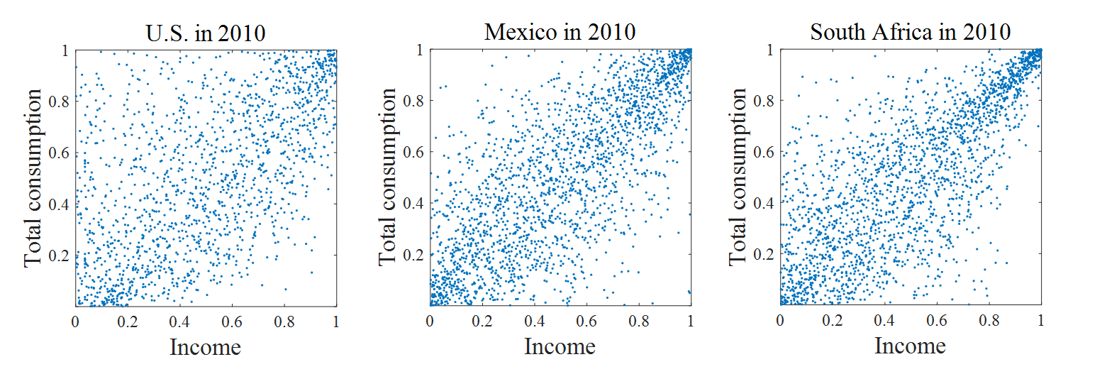
Figure 3: The figure displays the scatterplots of household income and consumption in 2010, in the U.S., Mexico, and South Africa after applying the probability integral transforms.

Here, we apply our test to the income and consumption data of the three countries. By applying our test procedure, we may detect difference in the degree of dependence between different group as well as a discrepancy in the structure of the dependence. In the comparison of the U.S., and Mexico, the test statistics are computed as $(T_{n,m}^{(2)},T_{n,m}^{(\infty)})=(1.49,3.32)$ and the p-values for both statistics turn out to be zero, suggesting that the dependence structures of income and consumption in the two countries are significantly different. In the comparison of Mexico and South Africa, the test statistics are computed as $(T_{n,m}^{(2)},T_{n,m}^{(\infty)})=(0.43,1.30)$. Surprisingly, our randomization test leads to zero p-values for both $T_{n,m}^{(2)}$ and $T_{n,m}^{(\infty)}$ despite that the correlation coefficients and Kendall’s $\tau$ are very similar in South Africa and Mexico. This indicates that a strong dissimilarity detected by our test procedure may not be detected by correlation coefficients or Kendall’s $\tau$.

$c$	U.S.		Mexico		South Africa
	lower $\tau$	upper $\tau$	lower $\tau$	upper $\tau$	lower $\tau$	upper $\tau$
0.2	0.033	0.192	0.200	0.378	0.128	0.431
0.3	0.116	0.205	0.247	0.407	0.178	0.489
0.4	0.163	0.240	0.292	0.435	0.213	0.527
0.5	0.198	0.264	0.337	0.454	0.248	0.546
0.6	0.235	0.282	0.374	0.473	0.291	0.557
0.7	0.284	0.316	0.421	0.494	0.344	0.557
0.8	0.330	0.359	0.466	0.521	0.409	0.558

Table 4: The table reports the upper and lower conditional Kendall’s $\tau$ of income and consumption in the U.S., Mexico and South Africa at exceedance levels $c\in\{0.2,0.3,0.4,0.5,0.6,0.7,0.8\}$.

Table 5.1 provides more detailed information on the structure of income and consumption dependence in the U.S., Mexico and South Africa in 2010. In the table, we report the conditional Kendall’s $\tau$ of income and consumption at several different exceedance levels. Recall that for a pair of random variables $(X,Y)$, Kendall’s $\tau$ is defined by $\tau(X,Y)=P((X_{i}-X_{j})(Y_{i}-Y_{j})>0)-P((X_{i}-X_{j})(Y_{i}-Y_{j})<0)$, where $(X_{i},Y_{i})$ and $(X_{j},Y_{j})$ are two random draws of $(X,Y)$. Then, the conditional Kendall’s $\tau$ at the exceedance level $c\in(0,1)$ is provided by

$$\tau^{-}(c) = \tau(F_{X}(X),F_{Y}(Y)|F_{X}(X)<c,F_{Y}(Y)<c)\text{\ \ and}$$

$$\tau^{+}(c) = \tau(F_{X}(X),F_{Y}(Y)|F_{X}(X)>1-c,F_{Y}(Y)>1-c).$$

We observe that in all three countries, the upper conditional dependence is stronger than the lower conditional dependence at any fixed exceedance level. It implies that within a country, the dependence patterns are different depending on relative income and consumption levels. In particular, we found that when both income and consumption levels are relatively low, a greater portion of consumption is on necessities, and the consumption of necessities does not increase much by an increase in the income. On the other hand, when both income and consumption levels are relatively high, consumers spend a greater portion of their income on luxury goods. Hence, the dependence between income and consumption tends to be stronger in the upper tail than in the lower tail.

In addition, Table 5.1 shows that both the upper conditional dependence and the lower conditional dependence are weaker in the U.S. than in Mexico and South Africa at all exceedance levels. This is consistent with our finding that the U.S. has the lowest correlation coefficient and the lowest Kendall’s $\tau$ among the three countries. On the other hand, compared to Mexico, South Africa has smaller lower conditional dependence but larger upper conditional dependence at any fixed exceedance level. As the surplus in upside dependence is offset by the deficit in downside dependence, the value of the correlation coefficients or Kendall’s $\tau$ may be similar to that of Mexico. Nevertheless, the patterns of asymmetric dependence in the two countries are very different, and our test procedure can distinguish the dissimilarity of such nonlinear patterns.

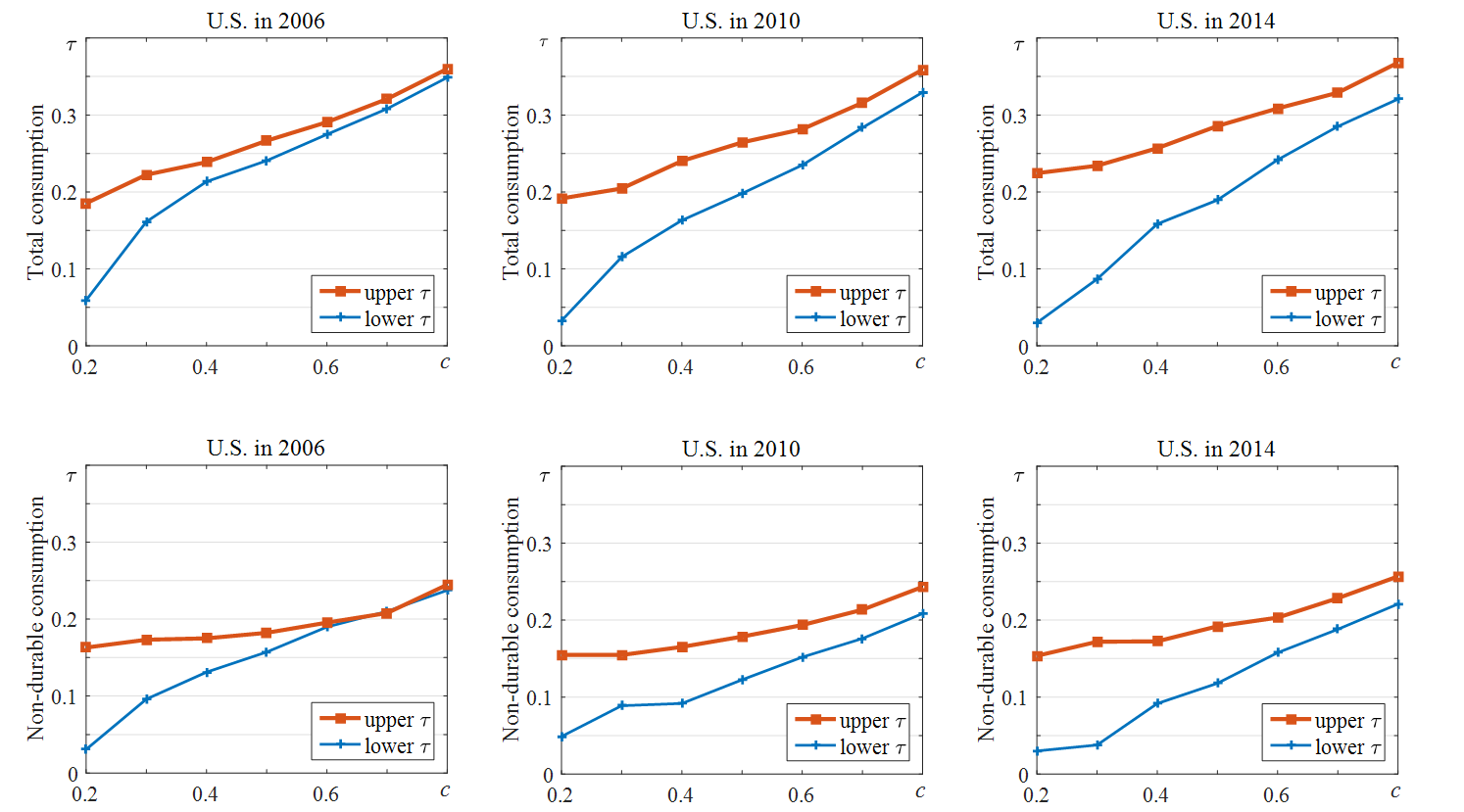
Figure 4: We display the graphs of the upper and lower conditional Kendall’s $\tau$ of income and consumption in the U.S. in 2006, 2010 and 2014. While the upper conditional dependence does not vary much over the three years, the lower conditional dependence tends to decrease over time.

Since the U.S. Consumer Expenditure Survey provides richer information than the Mexican and South African surveys, we may explore in more depth the recent changes in the income and consumption dependence in the U.S. Hence, we provide additional analysis on the dependence of income and total consumption in the U.S. in 2006, 2010 and 2014, as well as that of income and non-durable consumption in 2006, 2010 and 2014. Following the definition in Attanasio et al. (2012), we define the consumption of non-durable goods as the household expenditure on food, clothing, footwear and non-durable entertainment. Based on this definition, we find that the correlation coefficients of income and consumption are very similar in the three years; the correlation coefficients of income and total consumption are 0.5, 0.53 and 0.5 in 2006, 2010 and 2014 respectively, while those of income and non-durable consumption are 0.44, 0.41 and 0.37.

Figure 5.2 provides the graphs of the conditional Kendall’s $\tau$ of income and consumption in the U.S. in 2006, 2010 and 2014. For both total consumption and non-durable consumption, the upper conditional Kendall’s $\tau$ remains almost the same in the three years, while the lower conditional Kendall’s $\tau$ tends to decrease slightly over time. The decrease in the lower conditional dependence is more noticeable between 2006 and 2010 than between 2010 and 2014. Our inference results reflect this finding. In testing for equal dependence of total consumption and income between 2006 and 2010, our p-values for $T_{n,m}^{(2)}$ and $T_{n,m}^{(\infty)}$ are computed as 0.04 and 0.08, while they are 0.30 and 0.99 between 2010 and 2014. Using non-durable consumption, we obtain slightly smaller p-values. The p-values for $T_{n,m}^{(2)}$ and $T_{n,m}^{(\infty)}$ are 0.03 and 0.01 between 2006 and 2010, while they are 0.22 and 0.94 between 2010 and 2014. The results suggest that for both specifications of consumption, the dependence structure of income and consumption is significantly different between 2006 and 2010 at the $5\%$ and $10\%$ significance levels. However, the difference is less significant between 2010 and 2014.

5.2 Brexit effect on financial integration in Europe

Since established, the European Union (EU) has served as a coalition which fostered the integration of economic development among European countries. The economic integration has forced the economic decisions of the countries in the EU to be intimately dependent on each other. The countries have benefited from the upside gains but also suffered from the downside losses. Among others, the U.K. has played a central role in the decision making process of EU, providing a large portion of its budget over the past years. However, in pursuit of financial and political independence, the U.K. eventually announced ‘Brexit’ (Britain’s exit from the EU) in June of 2016. The term ‘Brexit’, which had been previously used for the potential exit of the U.K. from the EU, does not refer to a hypothetical situation anymore.

The announcement of Brexit created a huge external shock to the international economy. Following the announcement, there have been massive debates on what would happen to the U.K. and EU in the future. One of the major concerns is the impact of the U.K.’s decision on the economic integration in Europe. In this section, we aim to provide statistical evidence of the ‘Brexit effect’ on European financial market integration by investigating stock returns in the U.K., France, Germany and Switzerland. Although the process of Brexit is still ongoing and no definitive answer may be given to the question of the long run effect of Brexit, our findings in this section will provide evidence of the Brexit effect in its early and transitional stage.

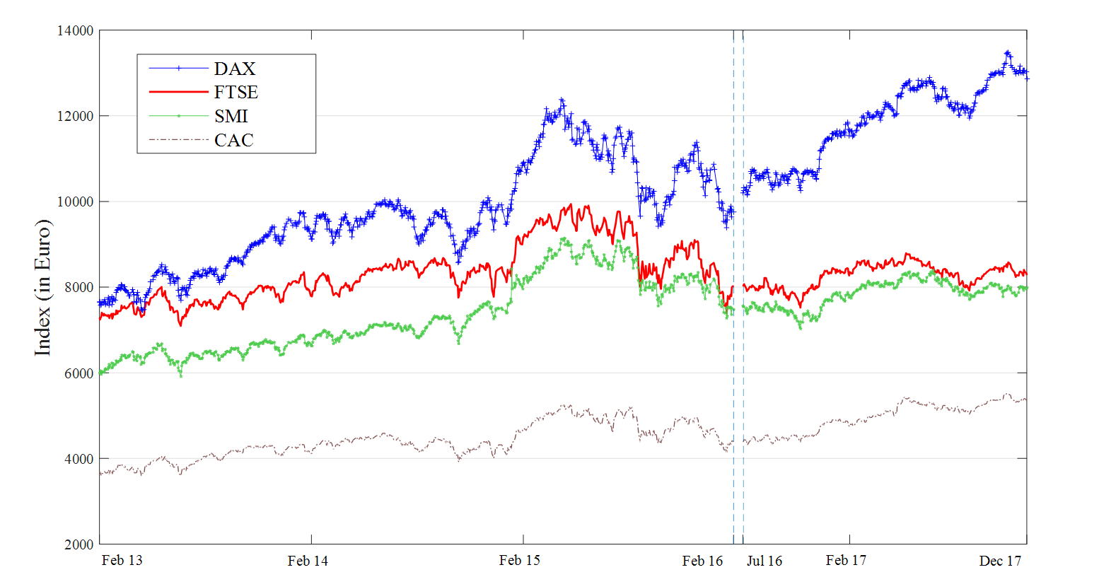
Figure 5: We display time plots of FTSE, CAC, DAX and SMI indices in the pre-Brexit and Brexit periods. The stock indices have a strong tendency to move together in both pre-Brexit and Brexit periods.

For our analysis, we collect the four stock indices of FTSE (U.K.), CAC (France), DAX (Germany) and SMI (Switzerland) from February 2013 to July 2017, at a daily frequency. Using the announcement of the Brexit as a cutoff point, we divide our observations into two groups, the data of ‘before’ the Brexit announcement and ‘after’ the Brexit announcement. To be more precise, we define the ‘pre-Brexit’ period as February 2013 through January 2016, and ‘Brexit’ period as July 2016 through December 2017. Although the referendum for Brexit was held in June 2016, the financial market structure in Europe has been potentially influenced by the announcement in February 2016 of making such a poll. Thus, we leave out the observations from February 2016 to June 2016 in defining the ‘pre-Brexit’ period. After excluding weekends and public holidays, the sample sizes are 734 for the pre-Brexit period and 338 for the Brexit period. These indices, as displayed in Figure 5.3, present a high degree of comovement in both pre-Brexit and Brexit periods. To remove temporal dependence, we apply the AR(1)-GJR-GARCH $(1,1)$ filter to the stock returns obtained by taking the log-difference of the indices.

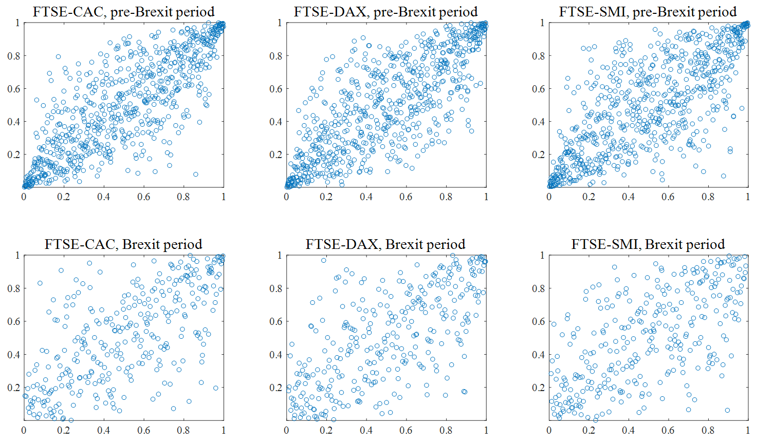
Figure 6: We display the scatterplots of the stock returns of FTSE against CAC, DAX, and SMI after applying the probability integral transformation. The three plots on the top illustrate the bivariate dependencies of FTSE and other stock returns in the pre-Brexit period and the three plots at the bottom illustrate those in the Brexit period.

Figure 5.4 displays scatterplots of the FTSE against CAC, DAX, and SMI in the pre-Brexit period and the Brexit period. The stock returns have been normalized by applying the probability integral transforms. Casual inspection reveals that the observations are less concentrated on the diagonal line in the Brexit period, suggesting that the cross market comovement of stock returns has become weaker after the U.K. decided to leave the EU. This can also be observed from the changes in the correlation coefficient. The correlation coefficient of FTSE and CAC is 0.86 in the pre-Brexit period and 0.71 in the Brexit period. Similarly, the correlation coefficients of FTSE and DAX, and of FTSE and SMI also have decreased from 0.82 to 0.65 and from 0.71 to 0.66, respectively.

stock returns	$T_{n,m}^{(2)}$	p-value	$T_{n,m}^{(\infty)}$	p-value
(FTSE, CAC)	0.253**	0.000	0.862**	0.000
(FTSE, DAX)	0.239**	0.000	0.731**	0.024
(FTSE, SMI)	0.143	0.154	0.599	0.234
(CAC, DAX)	0.124**	0.005	0.615**	0.048
(CAC, SMI)	0.144*	0.092	0.584	0.262
(DAX, SMI)	0.134	0.190	0.591	0.252
(CAC, DAX, SMI)	0.168**	0.048	0.721	0.237
(FTSE, CAC, DAX, SMI)	0.299**	0.002	1.036**	0.021

Table 5: The table shows the test statistics and p-values of our randomization test for equality in dependence structure. The null hypotheses concern the six pairwise dependence of (FTSE, CAC), (FTSE, DAX), (FTSE, SMI), (CAC, DAX), (CAC, SMI), (DAX, SMI), and the mutual dependence of (CAC, DAX, SMI), (FTSE, CAC, DAX, SMI). The critical values are obtained from 1000 random permutations to test each hypothesis.

In Table 5.2, we report our randomization test results concerning the Brexit effect. Firstly, our results show that the U.K.’s financial market dependence on the French and German financial markets has completely changed after the Brexit announcement. Applying our randomization test to the pairs of stock returns (FTSE, CAC) and (FTSE, DAX) yields p-values close to zero, which indicates overwhelming rejection of equality in the pairwise dependence. This change is due to the overall decrease in dependency (a change in the degree of dependence), and unequal decrease in dependency–more decrease in the downside than in the upside– that leads to asymmetric dependence (a change in the structure of dependence). For a fixed level $c=0.5$ for instance, the upper conditional Kendall’s $\tau$ of FTSE and CAC slightly decreased from $0.76$ to $0.65$ while the lower conditional Kendall’s $\tau$ substantially decreased from $0.77$ to $0.26$. In the (FTSE, DAX) pair, the upper conditional Kendall’s $\tau$ at level $c=0.5$ decreased from $0.44$ to $0.35$, while the lower conditional Kendall’s $\tau$ decreased from $0.43$ to $0.14$, and again, the decrease is more prominent in the downside than in the upside. On the other hand, the change of the dependence structure in the pair of (FTSE, SMI) turns out to be less significant: we fail to reject the null hypothesis of copula equality at both $5\%$ and $10\%$ significance levels. We also found that in terms of distributional symmetry, no obvious change in the pair (FTSE, SMI) is observed after the Brexit announcement.

While there is no universal consensus on the extension of the correlation coefficient or Kendall’s $\tau$ to more than two variables, our statistical procedure can be naturally applied to study higher dimensional dependence structures. For instance, by comparing the four dimensional copulas of stock returns to the FTSE, CAC, DAX, and SMI in the pre-Brexit and Brexit period, we can perform a statistical test to examine the Brexit effect on the dependence structure of the four returns. It turns out that our randomization tests with the statistics $T_{n,m}^{(2)}$ and $T_{n,m}^{(\infty)}$ yield p-values of $0.01$ and $0.02$ respectively, indicating that there has been a significance change in mutual dependence of the stock returns of FTSE, CAC, DAX, and SMI after the announcement of Brexit. Similarly, we can also examine the Brexit effect on the dependence of CAC, DAX and SMI, excluding FTSE. The question arises when our concern is to test for the Brexit effect on the financial market dependence among remaining EU countries. Here, our inference provides somewhat mixed results: we detect a significant change in the dependence structure of CAC, DAX and SMI with the test statistic $T_{n,m}^{(2)}$ at both $5\%$ and $10\%$ levels, but the change is less significant with $T_{n,m}^{(\infty)}$.

To summarize, our empirical findings reveal that the European financial market has experienced a substantial change after the Brexit announcement. Firstly, the dependence of financial market returns between the U.K. and other European countries has decreased after the Brexit announcement. In particular, we observe a greater decrease in dependence during market downturns than market upturns, which implies that the U.K.’s financial market is now less likely to crash together with other financial markets. Secondly, the financial integration among the U.K., France, Germany and Switzerland has decreased in reaction to the announcement of Brexit. Our test results indicate that there has been a significant change in the dependence structure of the stock markets in the four countries. We also found some evidence that the announcement of Brexit not only changed the financial market dependence of the U.K., but also that of the remaining EU countries. Lastly, the change in the dependence structure seems to be more recognizable among the larger economies. In our analysis, Brexit has caused more significant influence on financial market dependence among the U.K., France and Germany, while Switzerland has been less affected by the Brexit announcement.

6 Final remarks

Randomization tests provide useful tools for inference in situations where the null hypothesis implies that the distribution of the data is invariant to a group of transformations. In particular, permutation tests have been widely applied for testing the equality of distribution functions. Since copulas constitute a class of distribution functions, they may be naturally employed for testing the equality of copulas. However, the problem has not been examined to date and this is an important missing point in the literature.

This paper examines the use of permutation methods for testing copula equality. Unfortunately, the classical permutation method is not applicable because we do not observe samples directly from the copulas. Although we may instead explore the pseudo samples which consist of normalized ranks, the application of the permutation method still requires caution due to the distortion that permutation causes to the univariate margins of the pseudo samples. Asymptotically valid inference can be achieved by either modifying the permutation method considering the additional terms of the limit distribution induced by the uncertainty in margins (Theorem 3.1), or by correcting the distortion through taking one more step of normalizing the margins after each permutation (Theorem 3.2).

Appendix A Proofs and some numerical results

Lemma A.1. When $C_{1}=C_{2}$, the law of $\mathbb{\tilde{T}}\equiv\sqrt{1-\lambda}\mathbb{B}_{\bar{C}}-\sqrt{\lambda}\mathbb{B}_{\bar{C}}^{\prime}$ is equivalent to the law of $\mathbb{\tilde{T}}_{0}\equiv\sqrt{1-\lambda}\mathbb{B}_{C_{1}}-\sqrt{\lambda}\mathbb{B}_{C_{2}}$.

Proof of Lemma A.1. Since $\mathbb{\tilde{T}}$ and $\mathbb{\tilde{T}}_{0}$ are centered Gaussian processes, it suffices to show that their covariance structures are equivalent. We will prove it by showing that under the condition of $C_{1}=C_{2}$, each covariance kernel of $\mathbb{\tilde{T}}$ and $\mathbb{\tilde{T}}_{0}$ reduces to that of $\mathbb{B}_{C_{1}}$. Recall that $\mathbb{B}_{C_{1}}$ is a Brownian bridge on $[0,1]^{d}$ with covariance kernel

$$\text{Cov}\left(\mathbb{B}_{C_{1}}(\mathbf{u}),\mathbb{B}_{C_{1}}(\mathbf{u}^{\prime})\right)=C_{1}(\mathbf{u}\wedge\mathbf{u}^{\prime})-C_{1}(\mathbf{u})C_{1}(\mathbf{u}^{\prime})$$

for $\mathbf{u}$ and $\mathbf{u}^{\prime}$ in $[0,1]^{d}$.

Firstly, since $\mathbb{B}_{C_{1}}$ and $\mathbb{B}_{C_{2}}$ are independent, the covariance kernel of $\mathbb{\tilde{T}}_{0}$ can be written as,

$$\text{Cov}\left(\mathbb{\tilde{T}}_{0}(\mathbf{u}),\mathbb{\tilde{T}}_{0}(\mathbf{u}^{\prime})\right) = E\left\{\left(\sqrt{1-\lambda}\mathbb{B}_{C_{1}}(\mathbf{u})-\sqrt{\lambda}\mathbb{B}_{C_{2}}(\mathbf{u})\right)\left(\sqrt{1-\lambda}\mathbb{B}_{C_{1}}(\mathbf{u}^{\prime})-\sqrt{\lambda}\mathbb{B}_{C_{2}}(\mathbf{u}^{\prime})\right)\right\}$$

$$= (1-\lambda)\left(C_{1}(\mathbf{u}\wedge\mathbf{u}^{\prime})-C_{1}(\mathbf{u})C_{1}(\mathbf{u}^{\prime})\right)-\lambda\left(C_{2}(\mathbf{u}\wedge\mathbf{u}^{\prime})-C_{2}(\mathbf{u})C_{2}(\mathbf{u}^{\prime})\right)$$

$$= C_{1}(\mathbf{u}\wedge\mathbf{u}^{\prime})-C_{1}(\mathbf{u})C_{1}(\mathbf{u}^{\prime})$$

where the last equality follows from the condition $C_{1}=C_{2}$.

Second, using the independence of $\mathbb{B}_{\bar{C}}$ and $\mathbb{B}_{\bar{C}}^{\prime}$, the covariance kernel of $\mathbb{\tilde{T}}$ can be also written as,

$$\text{Cov}\left(\mathbb{\tilde{T}}(\mathbf{u}),\mathbb{\tilde{T}}(\mathbf{u}^{\prime})\right) = E\left\{\left(\sqrt{1-\lambda}\mathbb{B}_{\bar{C}}(\mathbf{u})-\sqrt{\lambda}\mathbb{B}_{\bar{C}^{\prime}}(\mathbf{u})\right)\left(\sqrt{1-\lambda}\mathbb{B}_{\bar{C}}(\mathbf{u}^{\prime})-\sqrt{\lambda}\mathbb{B}_{\bar{C}^{\prime}}(\mathbf{u}^{\prime})\right)\right\}$$

$$= (1-\lambda)(\bar{C}(\mathbf{u}\wedge\mathbf{u}^{\prime})-\bar{C}(\mathbf{u})\bar{C}(\mathbf{u}^{\prime}))-\lambda(\bar{C}(\mathbf{u}\wedge\mathbf{u}^{\prime})-\bar{C}(\mathbf{u})\bar{C}(\mathbf{u}^{\prime}))$$

$$= \bar{C}(\mathbf{u}\wedge\mathbf{u}^{\prime})-\bar{C}(\mathbf{u})\bar{C}(\mathbf{u}^{\prime})\text{\ \ \ \ \ \ }$$

$$= C_{1}(\mathbf{u}\wedge\mathbf{u}^{\prime})-C_{1}(\mathbf{u})C_{1}(\mathbf{u}^{\prime})$$

The last equality is from the condition that $C_{1}=C_{2}=\bar{C}$ (see Remark 3.1). This completes our proof.

Proof of Lemma 3.1. The proof is straightforward from an application of the continuous mapping theorem to the weak convergence of the empirical copula process.

Proof of Lemma 3.2. For any $\mathbf{u}=(u_{1},...,u_{d})\in[0,1]^{d}$, $\tilde{C}_{1,n}$ is linear in the sense that we may write

$$\sqrt{n}(\tilde{C}_{1,n}(Z)(\mathbf{u})-C_{1}(\mathbf{u}))=\frac{1}{\sqrt{n}}\sum_{i=1}^{n}\left\{1(U^{i}\leq\mathbf{u})-E(1(U^{i}\leq\mathbf{u}))\right\}\text{.\ }$$

Note that $\sqrt{n}(\tilde{C}_{1,n}(Z)-C_{1})$ is simply the standard empirical process, and the limit of $\sqrt{n}(\tilde{C}_{1,n}(Z)-C_{1})$ is the $C_{1}$-Brownian bridge, $\mathbb{B}_{C_{1}}$. The same point can be made with regard to any properly defined copula. Therefore, the empirical processes associated with $C_{2}$ and $\bar{C}$ are also linear and their limits are $\mathbb{B}_{C_{2}}$ and $\mathbb{B}_{\bar{C}}$, respectively. Then the remaining proof of Lemma 3.2 can be done by verifying the key conditions in Chung and Romano (2013).

Let $Q_{1}^{i}(Z)(\mathbf{u})=1(U^{i}\leq\mathbf{u})$ and $Q_{2}^{j}(Z)(\mathbf{u})=1(V^{j}\leq\mathbf{u})$ for $i=1,...,n$ and $j=1,...,m$, and let $\bar{Q}_{1,n}$ and $\bar{Q}_{2,m}$ be the sample means calculated from $\{Q_{1}^{i}\}_{i=1}^{n}$ and $\{Q_{2}^{j}\}_{j=1}^{m}$ respectively. We observe that $\tilde{T}_{n,m}(Z)$ is simply a scaled difference between the two sample means,

$$\tilde{T}_{n,m}(Z)=\sqrt{\frac{nm}{n+m}}\left(\bar{Q}_{1,n}(Z)-\bar{Q}_{2,m}(Z)\right)\text{,}$$

and the limit of its sampling distribution is $\sqrt{1-\lambda}\mathbb{B}_{C_{1}}-\sqrt{\lambda}\mathbb{B}_{C_{2}}$ under $C_{1}=C_{2}$. On the other hand, the limit of its permutation distribution can be inferred from its asymptotic unconditional distribution when the samples are drawn from that mixture distribution. Since the mixture distribution of $U=(U_{1},...,U_{d})$ and $V=(V_{1},...,V_{d})$ is the mixture of the copula of $U$ and $V$, i.e., $\bar{C}=\lambda C_{1}+(1-\lambda)C_{2}$, by Chung and Romano (2013) we have

$$(\tilde{T}_{n,m}(Z^{\pi}),\tilde{T}_{n,m}(Z^{\pi^{\prime}}))\rightsquigarrow(\mathbb{\tilde{T}},\mathbb{\tilde{T}}^{\prime})$$

where $\mathbb{\tilde{T}}$ is $\sqrt{1-\lambda}\mathbb{B}_{\bar{C}}-\sqrt{\lambda}\mathbb{B}_{\bar{C}}^{\prime}$ and $\mathbb{\tilde{T}}^{\prime}$ is an independent copy of $\mathbb{\tilde{T}}$. Note that the conditions (5.9) and (5.10) in Chung and Romano (2013) are trivially satisfied because this is simply the problem of the difference in means. The result is also consistent with Lemma 4.3 in Romano (1990) and Theorem 1 in Wu (1990).

Proof of Lemma 3.3. We start by noting that the specific form of $1(\hat{Z}^{i}\leq\mathbf{u})$ is determined by the range of $i$; $1(\hat{Z}^{i}\leq\mathbf{u})$ is $1(\hat{U}_{n}^{i}\leq\mathbf{u})$ for $1\leq i\leq n$, and $1(\hat{V}_{m}^{i-n}\leq\mathbf{u})$ for $n<i\leq N$. Motivated from this observation, we consider the following decomposition of $\tilde{T}_{n,m}(\hat{Z}^{\pi})$:

$$\tilde{T}_{n,m}(\hat{Z}^{\pi})(\mathbf{u}) = \sqrt{\frac{nm}{n+m}}\left\{\left(\frac{1}{n}\sum_{i=1}^{n}1(\hat{Z}^{\pi(i)}\leq\mathbf{u},\pi(i)\leq n)+\frac{1}{n}\sum_{i=1}^{n}1(\hat{Z}^{\pi(i)}\leq\mathbf{u},\pi(i)>n)\right)\right.$$

$$\left.-\left(\frac{1}{m}\sum_{i=n+1}^{N}1(\hat{Z}^{\pi(i)}\leq\mathbf{u},\pi(i)\leq n)+\frac{1}{m}\sum_{i=n+1}^{N}1(\hat{Z}^{\pi(i)}\leq\mathbf{u},\pi(i)>n)\right)\right\}$$

$$= \sqrt{\frac{nm}{n+m}}\left\{\left(\frac{1}{n}\sum_{i=1}^{n}1(\hat{Z}^{\pi(i)}\leq\mathbf{u},\pi(i)\leq n)-\frac{1}{m}\sum_{i=n+1}^{N}1(\hat{Z}^{\pi(i)}\leq\mathbf{u},\pi(i)\leq n)\right)\right.$$

$$\left.+\left(\frac{1}{n}\sum_{i=1}^{n}1(\hat{Z}^{\pi(i)}\leq\mathbf{u},\pi(i)>n)-\frac{1}{m}\sum_{i=n+1}^{N}1(\hat{Z}^{\pi(i)}\leq\mathbf{u},\pi(i)>n)\right)\right\}\text{. }$$

The first two terms in the last equation collect the terms of the form $1(\hat{U}_{n}^{i}\leq u)$ for $i=1,...,n$, and the last two terms in the last equation collect the terms of the form $1(\hat{V}_{m}^{j}\leq u)$ for $j=1,...,m$.

Now for $\pi\in\mathbf{G}_{N}$, define $\alpha_{n,m}^{\pi}(\mathbf{u})$ and $\beta_{n,m}^{\pi}(\mathbf{u})$ as

$$\alpha_{n,m}^{\pi}(\mathbf{u})=\sqrt{\frac{nm}{n+m}}\left(\frac{1}{n}\sum_{i=1}^{n}1(Z^{\pi(i)}\leq\mathbf{u},\pi(i)\leq n)-\frac{1}{m}\sum_{i=n+1}^{N}1(Z^{\pi(i)}\leq\mathbf{u},\pi(i)\leq n)\right)$$

and

$$\beta_{n,m}^{\pi}(\mathbf{u})=\sqrt{\frac{nm}{n+m}}\left(\frac{1}{n}\sum_{i=1}^{n}1(Z^{\pi(i)}\leq\mathbf{u},\pi(i)>n)-\frac{1}{m}\sum_{i=n+1}^{N}1(Z^{\pi(i)}\leq\mathbf{u},\pi(i)>n)\right)\text{. }$$

Using the notations $\alpha_{n,m}^{\pi}$ and $\beta_{n,m}^{\pi}$, we can rewrite $\tilde{T}_{n,m}(Z^{\pi})$ and $\tilde{T}_{n,m}(\hat{Z}^{\pi})$ in the following way. Let $D_{n}(\mathbf{u})=(D_{1,n}(u_{1}),...,D_{d,n}(u_{d}))$ and $E_{m}(\mathbf{u})=(E_{1,m}(u_{1}),...,E_{d,m}(u_{d}))$, where those components are defined by $D_{q,n}(u_{q})=\frac{1}{n}\sum_{i=1}^{n}1(F_{q}(X_{q}^{i})\leq u_{q})$ and $E_{q,m}(u_{q})=\frac{1}{m}\sum_{j=1}^{m}1(G_{q}(Y_{q}^{j})\leq u_{q})$. Let $D_{n}^{-1}$ and $E_{m}^{-1}$ be the componentwise generalized inverse, as in Rémillard and Scaillet (2009; 383p). Then, we have

$$\tilde{T}_{n,m}(Z^{\pi})(\mathbf{u}) = \alpha_{n,m}^{\pi}(\mathbf{u})+\beta_{n,m}^{\pi}(\mathbf{u})\text{ \ and}$$

$$\tilde{T}_{n,m}(\hat{Z}^{\pi})(\mathbf{u}) = \alpha_{n,m}^{\pi}(D_{n}^{-1}(\mathbf{u}))+\beta_{n,m}^{\pi}(E_{m}^{-1}(\mathbf{u})).$$

The joint convergence of $\alpha_{n,m}^{\pi}$ and $\beta_{n,m}^{\pi}$ can be shown using the same argument in Lehmann and Romano (2005; Example 15.2.6 and Theorem 15.2.5). To understand how, it helps to see how $\alpha_{n,m}^{\pi}$ and $\beta_{n,m}^{\pi}$ can be reformulated in their framework. The terms $\alpha_{n,m}^{\pi}$ and $\beta_{n,m}^{\pi}$ can be written in terms of $Q_{1}^{i}$ and $Q_{2}^{j}$ defined in our proof of Lemma 3.2. Let $\Gamma=(\Gamma^{1},\Gamma^{2},...,\Gamma^{N})=(Q_{1}^{1},...,Q_{1}^{n},0,...,0)$ and let $\Upsilon=(\Upsilon^{1},\Upsilon^{2},...,\Upsilon^{N})=(0,...,0,Q_{2}^{1},...,Q_{2}^{m})$. We have,

$$(\alpha_{n,m}^{\pi},\beta_{n,m}^{\pi})=\left(\sqrt{\frac{nm}{n+m}}\sum_{i=1}^{N}\Gamma^{i}\kappa^{\pi(i)},\sqrt{\frac{nm}{n+m}}\sum_{i=1}^{N}\Upsilon^{i}\kappa^{\pi(i)}\right)$$

where $\kappa^{\pi(i)}$ is defined to be $\frac{1}{n}$ when $\pi(i)\leq n$ and $-\frac{1}{m}$ otherwise.

Now, let the individual limits of $\alpha_{n,m}^{\pi}$ and $\beta_{n,m}^{\pi}$ be $\alpha^{\ast}$ and $\beta^{\ast}$ respectively. The triangular inequality implies that

$$\sup_{\mathbf{u}\in[0,1]^{d}}\left|\alpha_{n,m}^{\pi}(D_{n}^{-1}(\mathbf{u}))+\beta_{n,m}^{\pi}(E_{m}^{-1}(\mathbf{u}))-(\alpha^{\ast}(\mathbf{u})+\beta^{\ast}(\mathbf{u}))\right|$$

$$\leq \sup_{\mathbf{u}\in[0,1]^{d}}\left|\alpha_{n,m}^{\pi}(D_{n}^{-1}(\mathbf{u}))-\alpha^{\ast}(\mathbf{u})\right|+\sup_{\mathbf{u}\in[0,1]^{d}}\left|\beta_{n,m}^{\pi}(E_{m}^{-1}(\mathbf{u}))-\beta^{\ast}(\mathbf{u})\right|$$

where $\alpha^{\ast}+\beta^{\ast}$ is $\mathbb{\tilde{T}}$. Since $\sup_{\mathbf{u}\in[0,1]^{d}}\left|D_{n}^{-1}(\mathbf{u})-\mathbf{u}\right|\rightarrow 0$ and $\sup_{\mathbf{u}\in[0,1]^{d}}\left|E_{m}^{-1}(\mathbf{u})-\mathbf{u}\right|\rightarrow 0$ as $n$ and $m\rightarrow\infty$ (Shorack and Wellner, 1986; Rémillard and Scaillet, 2009), we conclude $\tilde{T}_{n,m}(\hat{Z}^{\pi})\rightsquigarrow\mathbb{\tilde{T}}$.

Lastly, consider a permutation $\pi^{\prime}\in\mathbf{G}_{N}$ that is independent of $\pi$. Let $\hat{Q}^{i}=1(\hat{Z}^{i}\leq\mathbf{u})$ for $i=1,...,N$ and $\kappa^{\pi^{\prime}(i)}$ be $\frac{1}{n}$ if $\pi^{\prime}(i)\leq n$ and $-\frac{1}{m}$ otherwise. Then, we see that

$$Cov(\tilde{T}_{n,m}(\hat{Z}^{\pi}),\tilde{T}_{n,m}(\hat{Z}^{\pi^{\prime}}))=\sqrt{\frac{nm}{n+m}}Cov\left(\sum_{i=1}^{N}\hat{Q}^{i}\kappa^{\pi(i)},\sum_{i=1}^{N}\hat{Q}^{i}\kappa^{\pi^{\prime}(i)}\right)=0\text{.}$$

The independence of $\mathbb{\tilde{T}}$ and $\mathbb{\tilde{T}}^{\prime}$ follows from the independence of $\pi$ and $\pi^{\prime}$, as in Lehmann and Romano (2005; 641p-642p).

Proof of Theorem 3.1. We invoke the Slutsky’s theorem for randomization distributions, treating copula derivatives as non-random constants for each $\mathbf{u}$. Let $\mathbb{C}_{0}=\sqrt{1-\lambda}\mathbb{C}_{C_{1}}-\sqrt{\lambda}\mathbb{C}_{C_{2}}$ and $\mathbb{C}_{0}^{\prime}$ be an independent copy of $\mathbb{C}_{0}$. By Lemma A.1, Lemma 3.3, Theorem 5.1 and Theorem 5.2 in Chung and Romano (2013), we have,

$$(\mathfrak{T}_{n,m}^{\pi},\mathfrak{T}_{n,m}^{\pi^{\prime}})\rightsquigarrow(\mathbb{C}_{0},\mathbb{C}_{0}^{\prime})$$

whenever $C_{1}=C_{2}$. In terms of conditional convergence, we have $\mathfrak{T}_{n,m}^{\pi}\overset{\mathrm{P}}{\underset{\pi}{\rightsquigarrow}}\mathbb{C}_{0}$ under the null hypothesis, and our proof is done by applying the continuous mapping theorem for the conditional convergence (Lemma A.2 below),

$$\left\|\mathfrak{T}_{n,m}^{\pi}\right\|_{p}\overset{\mathrm{P}}{\underset{\pi}{\rightsquigarrow}}\|\mathbb{C}_{0}\|_{p}=\mathbb{T}^{(p)}\text{.}$$

By Lemma 10.11 in Kosorok (2008), it follows that

$$P(\left\|\mathfrak{T}_{n,m}^{\pi}\right\|_{p}\leq c|\hat{Z})\xrightarrow{p}P(\mathbb{T}^{(p)}\leq c).$$

In what follows, we introduce our Lemma A.2 and Lemma A.3, which formalize the continuous mapping theorem and the conditional delta method for the conditional convergence. Lemma A.2 is a version of Theorem 10.8 of Kosorok (2008) and Lemma A.3 is obtained by extending the proof of Theorem 12.1 of Kosorok (2008) to the case where we have two independence copies of $\mathbb{X}_{1}$ and $\mathbb{X}_{2}$ in the limit, allowing that the laws of $\mathbb{X}_{1}$ and $\mathbb{X}_{2}$ to be different. See also Beare and Seo (2017).

Lemma A.2. (Continuous Mapping Theorem) Let $\mathbf{A}$ and $\mathbf{B}$ be Banach spaces. Define a continuous map $f:\mathbf{A}\rightarrow\mathbf{B}$ at all points in a closed set $\mathbf{A}_{0}\subset\mathbf{A}$. If $\xi_{N}^{\pi}\overset{\mathrm{P}}{\underset{\pi}{\rightsquigarrow}}\xi$ in $\mathbf{A}$, where $\xi$ is tight and concentrates on $\mathbf{A}_{0}$, then $f(\xi_{N}^{\pi})\overset{\mathrm{P}}{\underset{\pi}{\rightsquigarrow}}f(\xi)$ in $\mathbf{B}$.

Lemma A.3. (Conditional Delta Method) Let $\mathbf{A}$ and $\mathbf{B}$ be Banach spaces and let $f:\mathbf{A}_{f}\subset\mathbf{A}\rightarrow\mathbf{B}$ be Hadamard differentiable at $\mu\in\mathbf{A}_{f}$ tangentially to $\mathbf{A}_{0}\subset\mathbf{A}$, with derivative $f_{\mu}^{\prime}$. Further let $\eta(N)\,$be a rate of convergence and $\xi_{N}\in\mathbf{A}_{f}$ be an element which depends on the data but not $\pi$. If $\eta(N)(\xi_{N}-\mu)\rightsquigarrow\mathbb{X}_{1}$ and $\eta(N)(\xi_{N}^{\pi}-\xi_{N})\overset{\mathrm{P}}{\underset{\pi}{\rightsquigarrow}}\mathbb{X}_{2}$ in $\mathbf{A}$ with tight limits $\mathbb{X}_{1}$ and $\mathbb{X}_{2}$ in $\mathbf{A}_{0}$, we have $\eta(N)(f(\xi_{N}^{\pi})-f(\xi_{N}))\overset{\mathrm{P}}{\underset{\pi}{\rightsquigarrow}}f_{\mu}^{\prime}(\mathbb{X}_{2})\text{ in }\mathbf{B}$.

Proof of Lemma 3.4. Note that for $\mathbf{u}=(u_{1},...,u_{d})\in[0,1]^{d}$ and each $\pi\in\mathbf{G}_{N}$, we have

$$\tilde{T}_{n,m}(\hat{Z}^{\pi})(\mathbf{u}) = \sqrt{\frac{nm}{n+m}}\left(\frac{1}{n}\sum_{i=1}^{n}1(\hat{Z}^{\pi(i)}\leq\mathbf{u})-\frac{1}{m}\sum_{i=n+1}^{N}1(\hat{Z}^{\pi(i)}\leq\mathbf{u})\right)$$

$$= \sqrt{\frac{nm}{n+m}}\left(\frac{(n+m)}{nm}\sum_{i=1}^{n}1(\hat{Z}^{\pi(i)}\leq\mathbf{u})-\frac{1}{m}\sum_{i=1}^{N}1(\hat{Z}^{i}\leq\mathbf{u})\right)$$

$$= \sqrt{\frac{n(n+m)}{m}}\left[\tilde{C}_{1,n}^{\pi}(\mathbf{u})-\left\{\left(\frac{n}{n+m}\right)\hat{C}_{1,n}(\mathbf{u})+\left(\frac{m}{n+m}\right)\hat{C}_{2,m}(\mathbf{u})\right\}\right]\text{. \ \ }$$

Our condition on the rate of $\lambda_{n,m}$ implies $\lambda_{n,m}-\lambda=o(n^{-1/2})$. Therefore, from the last equation we obtain

$$\tilde{T}_{n,m}(\hat{Z}^{\pi})=\sqrt{n}(1-\lambda_{n,m})^{-1/2}\left\{\tilde{C}_{1,n}^{\pi}-(\lambda\hat{C}_{1,n}+\left(1-\lambda\right)\hat{C}_{2,m})\right\}+o_{p}(1)\text{.}$$

In the same way, we can also verify that

$$\tilde{T}_{n,m}(\hat{Z}^{\pi})=\sqrt{m}(\lambda_{n,m})^{-1/2}\left\{\left(\lambda\hat{C}_{1,n}+\left(1-\lambda\right)\hat{C}_{2,m}\right)-\tilde{C}_{2,m}^{\pi}\right\}+o_{p}(1)\text{.}$$

employing the condition

$\lambda_{n,m}-\lambda=o(m^{-1/2})$.

In view of the conditional convergence, let $\pi$ be a random permutation uniform on $\mathbf{G}_{N}$, and let $\Psi_{n,m}^{1,\pi}$ and $\Psi_{n,m}^{2,\pi}$ be rescaled versions of the non-decaying terms,

$$\Psi_{n,m}^{1,\pi} = \sqrt{\frac{nm}{n+m}}\left\{\tilde{C}_{1,n}^{\pi}-\left(\lambda\hat{C}_{1,n}+\left(1-\lambda\right)\hat{C}_{2,m})\right)\right\}\text{ and}$$

$$\Psi_{n,m}^{2,\pi} = \sqrt{\frac{nm}{n+m}}\left\{\left(\lambda\hat{C}_{1,n}+\left(1-\lambda\right)\hat{C}_{2,m}\right)-\tilde{C}_{2,m}^{\pi}\right\}\text{. }$$

The conditional convergence of $\Psi_{n,m}^{1,\pi}$ and $\Psi_{n,m}^{2,\pi}$ can be obtained by Lemma 3.3 as,

$$\left(\begin{array}[]{c}(1-\lambda_{n,m})\tilde{T}_{n,m}(\hat{Z}^{\pi})\\ \lambda_{n,m}\tilde{T}_{n,m}(\hat{Z}^{\pi})\end{array}\right)=\left(\begin{array}[]{c}\Psi_{n,m}^{1,\pi}+r_{n,m}^{(1)}\\ \Psi_{n,m}^{2,\pi}+r_{n,m}^{(2)}\end{array}\right)\text{ }\overset{\mathrm{P}}{\underset{\pi}{\rightsquigarrow}}\left(\begin{array}[]{c}(1-\lambda)\mathbb{\tilde{T}}\\ \lambda\mathbb{\tilde{T}}\end{array}\right)$$ (14)

in which both $r_{n,m}^{(1)}$ and $r_{n,m}^{(2)}$ are $o_{p}(1)$, and asymptotically negligible.

We finish our proof by applying Lemma A.2 and Lemma A.3 to the result in (14). Note that the two following two conditions (i) and (ii) are satisfied for an application of the conditional functional delta method,

$$\text{(i) }\Psi_{n,m}^{1,\pi}\overset{\mathrm{P}}{\underset{\pi}{\rightsquigarrow}}(1-\lambda)\mathbb{\tilde{T}}\text{ \ and \ }\Psi_{n,m}^{2,\pi}\overset{\mathrm{P}}{\underset{\pi}{\rightsquigarrow}}\lambda\mathbb{\tilde{T}}\text{ \ \ \ \ \ \ \ \ \ \ \ \ \ \ \ \ \ \ \ \ \ \ \ \ }$$

$$\text{(ii) }\sqrt{\frac{nm}{n+m}}\left(\lambda\hat{C}_{1,n}+\left(1-\lambda\right)\hat{C}_{2,m}-\left(\lambda C_{1}+\left(1-\lambda\right)C_{2}\right)\right) \rightsquigarrow \lambda\sqrt{1-\lambda}\mathbb{C}_{1}-(1-\lambda)\sqrt{\lambda}\mathbb{C}_{2},$$

and we obtain

$$\left(\begin{array}[]{c}\sqrt{\frac{nm}{n+m}}\left\{\Phi(\tilde{C}_{1,n}^{\pi})-\Phi\left(\lambda\hat{C}_{1,n}+\left(1-\lambda\right)\hat{C}_{2,m})\right)\right\}\\ \text{\ }\sqrt{\frac{nm}{n+m}}\left\{\Phi\left(\lambda\hat{C}_{1,n}+\left(1-\lambda\right)\hat{C}_{2,m}\right)-\Phi(\tilde{C}_{2,m}^{\pi})\right\}\end{array}\right)\text{ }\overset{\mathrm{P}}{\underset{\pi}{\rightsquigarrow}}\left(\begin{array}[]{c}(1-\lambda)\Phi_{\lambda C_{1}+(1-\lambda)C_{2}}^{\prime}\mathbb{\tilde{T}}\\ \lambda\Phi_{\lambda C_{1}+(1-\lambda)C_{2}}^{\prime}\mathbb{\tilde{T}}\end{array}\right)\text{.}$$

By the linearity of Hadamard derivatives we have

$$\sqrt{\frac{nm}{n+m}}\left(\Phi(\tilde{C}_{1,n}^{\pi})-\Phi(\tilde{C}_{2,m}^{\pi})\right)\overset{\mathrm{P}}{\underset{\pi}{\rightsquigarrow}}\Phi_{\lambda C_{1}+(1-\lambda)C_{2}}^{\prime}\mathbb{\tilde{T}}\text{.}$$

Proof of Theorem 3.2. Lemma A.1 and Lemma 3.4 imply that under the null hypothesis, we have

$$\sqrt{\frac{nm}{n+m}}\left(\Phi(\tilde{C}_{1,n}^{\pi})-\Phi(\tilde{C}_{2,m}^{\pi})\right)\overset{\mathrm{P}}{\underset{\pi}{\rightsquigarrow}}\Phi_{\lambda C_{1}+(1-\lambda)C_{2}}^{\prime}\mathbb{\tilde{T}}_{0}\text{.}$$

By using the same techniques as in Lemma 4.2 and Lemma 4.3 of Beare and Seo (2017), we can verify that $\Phi(\tilde{C}_{1,n}^{\pi})$ differs from $\hat{C}_{1,n}^{\pi}$ by no more than $2n^{-1}$ and $\Phi(\tilde{C}_{2,m}^{\pi})$ differs from $\hat{C}_{2,m}^{\pi}$ by no more than $2m^{-1}$. This concludes,

$$\sqrt{\frac{nm}{n+m}}(\hat{C}_{1,n}^{\pi}-\hat{C}_{2,m}^{\pi})\overset{\mathrm{P}}{\underset{\pi}{\rightsquigarrow}}\Phi_{\lambda C_{1}+(1-\lambda)C_{2}}^{\prime}\mathbb{\tilde{T}}_{0}\text{.}$$

Now applying our Lemma A.2 and Lemma 10.11 in Kosorok (2008), we have

$$P(\left\|\mathfrak{R}_{n,m}^{\pi}\right\|_{p}\leq c|\hat{Z})\xrightarrow{p}P(\mathbb{T}^{(p)}\leq c)$$

for any continuity points $c\in(0,\infty)$. Therefore, the result (i) in Theorem 3.2 follows. Next, suppose that the null hypothesis is false. Then by Lemma 3.4 and Lemma A.2, the permutation distribution of $\left\|\mathfrak{R}_{n,m}^{\pi}\right\|_{p}$ converges to $\|\Phi_{\lambda C_{1}+(1-\lambda)C_{2}}^{\prime}\mathbb{\tilde{T}}\|_{p}$, and the result (ii) in Theorem 3.2 follows from the divergence of $T_{n,m}^{(p)}$.

References

- Aas, K., Czado, C., Frigessi, A. and Bakken, H. (2009) Aas, K., Czado, C., Frigessi, A. and Bakken, H. (2009). Pair-copula constructions of multiple dependence. Insurance: Mathematics and economics 44(2) 182–198.
- Abhyankar, A., Copeland, L. S. and Wong, W. (1997) Abhyankar, A., Copeland, L. S. and Wong, W. (1997). Uncovering nonlinear structure in real-time stock-market indexes: the S&P 500, the DAX, the Nikkei 225, and the FTSE 100. Journal of Business & Economic Statistics 15(1) 1–14.
- Aloui, R., Aïssa, M. S. B. and Nguyen, D. K. (2011) Aloui, R., Aïssa, M. S. B. and Nguyen, D. K. (2011). Global financial crisis, extreme interdependences, and contagion effects: the role of economic structure? Journal of Banking & Finance 35(1) 130–141.
- Ando (1963) Ando, A. and Modigliani, F. (1963). The “life cycle” hypothesis of saving: aggregate implications and tests. American Economic Review 53(1) 55–84.
- Ang (2002) Ang, A. and Chen, J. (2002). Asymmetric correlations of equity portfolios. Journal of Financial Economics 63(3) 443–494.
- Attanasio (2012) Attanasio, O., Hurst, E. and Pistaferri, L. (2012). The evolution of income, consumption, and leisure inequality in the U.S., 1980-2010. National Bureau of Economic Research working paper. No. 17982.
- Beare (2010) Beare, B. K. (2010). Copulas and temporal dependence. Econometrica 78 395–410.
- Beare (2014) Beare, B. K. and Seo, J. (2014). Time irreversible copula-based Markov models. Econometric Theory 30(5) 923–960.
- Beare (2015) Beare, B. K. and Seo, J. (2015). Vine copula specifications for stationary multivariate Markov chains. Journal of Time Series Analysis 36 228–246.
- Beare (2017) Beare, B. K. and Seo, J. (2017). Quasi-randomization tests of copula symmetry. Preprint, UC San Diego.
- Bonhomme (2009) Bonhomme, S. and Robin, J. M. (2009). Assessing the equalizing force of mobility using short panels: France, 1990–2000. Review of Economic Studies 76(1) 63–92.
- Browning (2001) Browning, M. and Collado, M. D. (2001). The response of expenditures to anticipated income changes: panel data estimates. American Economic Review 91(3) 681–692.
- Bücher (2010) Bücher, A. and Dette, H. (2010). A note on bootstrap approximations for the empirical copula process. Statistics & Probability Letters 80 1925–1932.
- Bücher and Volgushev (2013) Bücher, A. and Volgushev, S. (2013). Empirical and sequential copula processes under serial dependence. Journal of Multivariate Analysis, 119 61–70.
- Campbell (1989) Campbell, J. and Deaton, A. (1989). Why is consumption so smooth? The Review of Economic Studies 56(3) 357–373.
- Campbell (1991) Campbell, J. and Mankiw, N. G. (1991). The response of consumption to income: a cross-country investigation. European economic review 35(4) 723–756.
- Canay (17) Canay, I. A., Romano, J. P. and Shaikh, A. M. (2017). Randomization tests under an approximate symmetry assumption. Econometrica 85 1013–1030.
- Chan, N. H., Chen, J., Chen, X., Fan, Y. and Peng, L. (2009) Chan, N. H., Chen, J., Chen, X., Fan, Y. and Peng, L. (2009). Statistical inference for multivariate residual copula of GARCH models. Statistica Sinica 53–70.
- Chen (2006) Chen, X. and Fan, Y (2006). Estimation of copula-based semiparametric time series models. Journal of Econometrics 130 307–335.
- Chen (2009) Chen, X., Wu, W. B. and Yi, Y (2009). Efficient estimation of copula-based semiparametric Markov models. The Annals of Statistics 37 4221–4253.
- Chung (2013) Chung, E. and Romano, J. P. (2013). Exact and asymptotically robust permutation tests. The Annals of Statistics 41 484–507.
- Chung, E., and Romano, J. P. (2016) Chung, E., and Romano, J. P. (2016). Multivariate and multiple permutation tests. Journal of Econometrics 193(1), 76-91.
- Cotter, J. (2007) Cotter, J. (2007). Varying the VaR for unconditional and conditional environments. Journal of International Money and Finance 26(8) 1338–1354.
- Creal, D. D., and Tsay, R. S. (2015) Creal, D. D., and Tsay, R. S (2015). High dimensional dynamic stochastic copula models. Journal of Econometrics 189(2) 335-345.
- Deheuvels (1981a) Deheuvels, P. (1981a). A Kolmogorov–Smirnov type test for independence and multivariate samples. Revue Roumaine de Mathématiques Pures et Appliquées 26 213–226.
- Deheuvels (1981b) Deheuvels, P. (1981b). A nonparametric test for independence. Publications de l’Institut de Statistique de l’Université Paris 26 29–50.
- Embrechts (2002) Embrechts, P., McNeil, A. and Straumann, D. (2002). Correlation and dependence in risk management: properties and pitfalls. Risk management: value at risk and beyond 176–223.
- Fermanian et al. (2004) Fermanian, J. D., Radulović, D. and Wegkamp, M. (2004). Weak convergence of empirical copula processes. Bernoulli 10 847–860.
- Flavin (1981) Flavin, M. A. (1981). The adjustment of consumption to changing expectations about future income. Journal of Political Economy 89(5) 974–1009.
- Friedman (1957) Friedman, M. (1957). Theory of the consumption function. Princeton University Press, Princeton.
- Gaenssler (1987) Gaenssler, P. and Stute, W. (1987). Seminar on Empirical Processes, DMV Sem. 9. Basel: Birkhäuser.
- Genest (2012) Genest, C., Nešlehová, J. G. and Quessy, J.F. (2012). Tests of symmetry for bivariate copulas. Annals of the Institute of Statistical Mathematics 64 811–834.
- Genest and Nešlehová (2014) Genest, C. and Nešlehová, J. G. (2014). On tests of radial symmetry for bivariate copulas. Statistical Papers 55 1107–1119.
- Giacomini, E., Härdle, W. and Spokoiny, V. (2009) Giacomini, E., Härdle, W. and Spokoiny, V. (2009). Inhomogeneous dependence modeling with time-varying copulae. Journal of Business & Economic Statistics 27(2) 224–234.
- Gine (2009) Giné, X. and Yang, D. (2009). Insurance, credit, and technology adoption: field experimental evidence from Malawi. Journal of development Economics 89(1) 1-11.
- Hall (1978) Hall, R. E. (1978). Stochastic implications of the Life Cycle-Permanent Income Hypothesis: theory and evidence. Journal of Political Economy 86(6) 971–987.
- Hall (1982) Hall, R. E. and Mishkin, F. S. (1982). The sensitivity of consumption to transitory Income: estimates from panel data on households. Econometrica 50(2) 461–481.
- Hoeffding (1952) Hoeffding, W. (1952). The large-sample power of tests based on permutations of obervations. The Annals of Mathematical Statistics 23 169–192.
- Hong (2001) Hong, Y., Tu, J. and Zhou, G. (2006). Asymmetries in stock returns: statistical tests and economic evaluation. The Review of Financial Studies 20(5) 1547–1581.
- Hsieh (2003) Hsieh, C. T. (2003). Do consumers react to anticipated income changes? Evidence from the Alaska permanent fund. American Economic Review 93(1) 397–405.
- Hu, L. (2006) Hu, L. (2006). Dependence patterns across financial markets: a mixed copula approach. Applied financial economics 16(10) 717–729.
- Hu, W. and Kercheval, A. N. (2010) Hu, W. and Kercheval, A. N. (2010). Portfolio optimization for student t and skewed t returns. Quantitative Finance 10(1) 91–105.
- Ibragimov (2009) Ibragimov, R. (2009). Copula-based characterizations for higher-order Markov processes. Econometric Theory 25 819–846.
- Janssen (1997) Janssen, A. (1997). Studentized permutation tests for non-i.i.d. hypotheses and the generalized Behrens–Fisher problem. Statistics & Probability Letters 36 9–21.
- Janssen (1999) Janssen, A. (1999). Testing nonparametric statistical functionals with applications to rank tests. Journal of Statistical Planning and Inference 81 71–93.
- Janssen (2005) Janssen, A. (2005). Resampling Student’s t-type statistics. Annals of the Institute of Statistical Mathematics 57 507–529.
- Janssen (2003) Janssen, A. and Pauls, T. (2003). How do bootstrap and permutation tests work? The Annals of Statistics 31 768–806.
- Janssen (2005) Janssen, A. and Pauls, T. (2005). A Monte Carlo comparison of studentized bootstrap and permutation for heteroscedastic two-sample problems. Computational Statistics 20 369–383.
- Jappelli (1989) Jappelli, T. and Pagano, M. (1989). Consumption and capital market imperfections: an international comparison. American Economic Review 79(5) 1088-1105.
- Johnson (2006) Johnson, D. S., Parker, J. A. and Souleles, N. S. (2006). Household expenditure and the income tax rebates of 2001. American Economic Review 96(5) 1589–1610.
- Kaplan (2014) Kaplan, G. and Violante, G. L. (2014). A model of the consumption response to fiscal stimulus payments. Econometrica 82(4) 1199–1239.
- Karlan (2014) Karlan, D., Osei, R., Osei-Akoto, I. and Udry, C. (2014). Agricultural decisions after relaxing credit and risk constraints. The Quarterly Journal of Economics 129(2) 579-652.
- Keynes (1936) Keynes, J. M. (1936). The General Theory of Employment, Interest and Money. Macmillan and co., London.
- Kojadinovic (2011) Kojadinovic, I. and Yan, J. (2011). A goodness-of-t test for multivariate multiparameter copulas based on multiplier central limit theorems. Statistics and Computing 21 17–30.
- Kojadinovic (2011) Kojadinovic, I., Yan, J. and Holmes, M. (2011). Fast large-sample goodness-of-fit tests for copulas. Statistica Sinica 21 841–871.
- Kosorok (2008) Kosorok, M. R. (2008). Introduction to Empirical Processes and Semiparametric Inference. Springer Series in Statistics, New York.
- Lee, T. H., and Long, X. (2009) Lee, T. H., and Long, X. (2009). Copula-based multivariate GARCH model with uncorrelated dependent errors. Journal of Econometrics 150(2) 207-218.
- Lehmann (2005) Lehmann, E. L. and Romano, J. P. (2005). Testing statistical hypotheses. Springer Science & Business Media.
- Loaiza-Maya, R., Smith, M. S., and Maneesoonthorn, W. (2018) Loaiza-Maya, R., Smith, M. S., and Maneesoonthorn, W. (2018). Time series copulas for heteroskedastic data. Journal of Applied Econometrics 33(3) 332-354.
- Longin (2001) Longin, F. and Solnik, B. (2001). Extreme correlation of international equity markets. The Journal of Finance 56(2) 649–676.
- Manner (2001) Manner, H. (2001). Testing for asymmetric dependence. Studies in Nonlinear Dynamics and Econometrics 14(2) 1–32.
- Neubert (2007) Neubert, K. and Brunner, E. (2007). A studentized permutation test for the non-parametric Behrens–Fisher problem. Computational Statistics & Data Analysis 51 5192–5204.
- Neuhaus (1993) Neuhaus, G. (1993). Conditional rank tests for the two-sample problem under random censorship. The Annals of Statistics 21 1760–1779.
- Nikoloulopoulos, A. K., Joe, H. and Li, H. (2012) Nikoloulopoulos, A. K., Joe, H. and Li, H. (2012). Vine copulas with asymmetric tail dependence and applications to financial return data. Computational Statistics & Data Analysis 56(11) 3659–3673.
- Oh (2013) Oh, D. H. and Patton, A. J. (2013). Simulated method of moments estimation for copula-based multivariate models. Journal of the American Statistical Association 108 689–700.
- Oh (2017) Oh, D. H. and Patton, A. J. (2017). Modeling dependence in high dimensions with factor copulas. Journal of Business & Economic Statistics 35 139–154.
- Omelka (2012) Omelka, M. and Pauly, M. (2012). Testing equality of correlation coefficients in two populations via permutation methods. Journal of Statistical Planning and Inference 142 1396–1406.
- Parker (1999) Parker, J. A. (1999). The reaction of household consumption to predictable changes in social security taxes. American Economic Review 89(4) 959–973.
- Parker (2013) Parker, J. A., Souleles, N. S., Johnson, D. S. and McClelland, R. (2013). Consumer spending and the economic stimulus payments of 2008. American Economic Review 103(6) 2530–2553.
- Patton (2006) Patton, A. J. (2006). Modelling asymmetric exchange rate dependence. International Economic Review 47 527–556.
- Rémillard and Scaillet (2009) Rémillard, B. and Scaillet, O. (2009). Testing for equality between two copulas. Journal of Multivariate Analysis 100 377–386.
- Romano (1989) Romano, J. P. (1989). Bootstrap and randomization tests of some nonparametric hypotheses. The Annals of Statistics 141-159.
- Romano (1990) Romano, J. P. (1990). On the behavior of randomization tests without a group invariance assumption. Journal of the American Statistical Association 85 686–692.
- Rosenberg (2006) Rosenberg, J. V. and Schuermann, T. (2006). A general approach to integrated risk management with skewed, fat-tailed risks. Journal of Financial economics 79 569–614.
- Rosenzweig (1993) Rosenzweig, M. R. and Wolpin, K. I. (1993). Credit market constraints, consumption smoothing, and the accumulation of durable production assets in low-income countries: investments in bullocks in India. Journal of political economy 101(2) 223-244.
- Sargent (1978) Sargent, T. J. (1978). Rational expectations, econometric exogeneity, and consumption. Journal of Political Economy 86(4) 673–700.
- Scaillet (2005) Scaillet, O. (2005). A kolmogorov-Smirnov type test for positive quadrant dependence. Canadian Journal of Statistics 33 415–427.
- Segers (2012) Segers, J. (2012). Asymptotics of empirical copula processes under non-restrictive smoothness assumptions. Bernoulli 18 764—782.
- Shapiro (1995) Shapiro, M. D. and Slemrod, J. (1995). Consumer response to the timing of income: evidence from a change in tax withholding. American Economic Review 85(1) 274–283.
- Shea (1995) Shea, J. (1995). Union contracts and the Life-Cycle/Permanent-Income Hypothesis. American Economic Review 85(1) 186–200.
- Sklar, M. (1959) Sklar, M. (1959). Fonctions de répartition à n dimensions et leurs marges. Publ. Inst. Statist. Univ. Paris 8 229–231.
- Smiths (2010) Smith, M., Min, A., Almeida, C., and Czado C. (2010). Modeling longitudinal data using a pair-copula decomposition of serial dependence. Journal of the American Statistical Association 105 1467-1479.
- Souleles (1999) Souleles, N. S (1999). The response of household consumption to income tax refunds. American Economic Review 89(4) 947–958.
- Tsukahara (2005) Tsukahara, H. (2005). Semiparametric estimation in copula models. Canadian Journal of Statistics 33 357–375.
- van der Vaart (1996) van der Vaart, A. W. and Wellner, J. A. (1996). Weak convergence and empirical processes. Springer–Verlag, New York.
- van der Vaart (2007) van der Vaart, A. W. and Wellner, J. A. (2007). Empirical processes indexed by estimated functions. Lecture Notes-Monograph Series 234–252.
- Wu (1990) Wu, C. F. (1990). On the asymptotic properties of the jackknife histogram. The Annals of Statistics 18 1438–1452.
- Zimmer (2006) Zimmer, D. M. and Trivedi, P. K. (2006). Using trivariate copulas to model sample selection and treatment effects: application to family health care demand. Journal of Business & Economic Statistics 24 63–76.
- Zimmerman (2003) Zimmerman, F. J. and Carter, M. R. (2003). Asset smoothing, consumption smoothing and the reproduction of inequality under risk and subsistence constraints. Journal of Development Economics 71(2) 233–260.