Structural nonequilibrium forces in driven colloidal systems

Abstract

We identify a structural one-body force field that sustains spatial inhomogeneities in nonequilibrium overdamped Brownian many-body systems. The structural force is perpendicular to the local flow direction, it is free of viscous dissipation, it is microscopically resolved in both space and and time, and it can stabilize density gradients. From the time evolution in the exact (Smoluchowski) low-density limit, Brownian dynamics simulations and a novel power functional approximation, we obtain a quantitative understanding of viscous and structural forces, including memory and shear migration.

It is a very significant challenge of Statistical Physics to rationalize and predict nonequilibrium structure formation from a microscopic starting point. Primary examples include shear banding dhont1999 ; dhont2003 ; dhont2014 , where spatial regions of different shear rate coexist, laning transitions in oppositely driven colloids laningLitOne ; laningLitTwo , where regions of different flow direction occur, as well as migration effects in inhomogeneous shear flow braderkrueger11epl ; braderkrueger11molphys ; reinhardt2013 ; aerov2014 ; aerov2015 ; scacchi2016 . In computer simulations, discriminating true steady states from slow initial transients can be difficult zausch2008 ; harrer2012 . Often the nonequilibrium structuring effects have associated long time scales and strong correlations Bolhuis2015 ; zimmermann16 . The underlying equilibrium phase diagram and bulk structure might already be complex and interfere with the genuine nonequilibrium effects floating ; empty .

To identify commonalities of all of the above situations, we investigate here a representative model situation. We put forward a systematic classification of the occurring nonequilibrium forces and identify a structural force component, which is able to sustain density gradients without creating dissipation. The structural force is solely due to the interaction between the particles, and it is hence of a nature different than that of the lift forces in hydrodynamics. We rationalize our findings by constructing an explicit power functional approximation, (15) below.

We restrict ourselves to overdamped Brownian dynamics and consider the microscopically resolved position- and time-dependent one-body density, $\rho({\mathbf{r}},t)$, and one-body current, ${\bf J}({\mathbf{r}},t)$. Both fields are related via the (exact) continuity equation $\partial\rho/\partial t=-\nabla\cdot{\bf J}$; here $\nabla$ indicates the derivative with respect to position ${\mathbf{r}}$. The velocity profile is simply the ratio ${\bf v}({\mathbf{r}},t)={\bf J}({\mathbf{r}},t)/\rho({\mathbf{r}},t)$.

The exact time evolution, with no hydrodynamic interactions present, can then be expressed by the one-body force balance equation

$$\gamma{\bf v} ={\bf f}_{\rm int}+{\bf f}_{\rm ext}-k_{B}T\nabla\ln\rho,$$ (1)

where $\gamma$ is the single-particle friction constant against the (implicit) solvent, ${\bf f}_{\rm int}({\mathbf{r}},t)$ is the internal force field, ${\bf f}_{\rm ext}({\mathbf{r}},t)$ is a one-body external force field that in general drives the system out of equilibrium, and $-k_{B}T\nabla\ln\rho({\mathbf{r}},t)\equiv{\bf f}_{\rm aid}({\mathbf{r}},t)$ is the adiabatic ideal gas contribution due to the free thermal diffusion; here $k_{B}$ is the Boltzmann constant and $T$ is absolute temperature. The internal force field ${\bf f}_{\rm int}({\mathbf{r}},t)$ arises from the interparticle interaction potential $u({\mathbf{r}}^{N})$, where ${\mathbf{r}}^{N}\equiv{\mathbf{r}}_{1}\ldots{\mathbf{r}}_{N}$ denotes the set of all position coordinates, and it can be expressed as an average over the interparticle one-body force density “operator”

$$\hat{\bf F}_{\rm int} =-\sum_{i}\delta({\mathbf{r}}-{\mathbf{r}}_{i})\nabla_{i}u({\mathbf{r}}^{N}),$$ (2)

where the sum is over all particles, $\delta(\cdot)$ indicates the Dirac distribution and $\nabla_{i}$ denotes the derivative with respect to ${\mathbf{r}}_{i}$. Using the probability distribution $\Psi({\mathbf{r}}^{N},t)$ of finding microstate ${\mathbf{r}}^{N}$ at time $t$, the average is built according to

$${\bf f}_{\rm int}({\mathbf{r}},t) =\rho({\mathbf{r}},t)^{-1}\int d{\mathbf{r}}^{N}\Psi({\bf r}^{N}\!\!,t)\hat{\bf F}_{\rm int},$$ (3)

where the normalization is performed using the time-dependent one-body density, defined as the average

$$\rho({\mathbf{r}},t)=\int d{\mathbf{r}}^{N}\Psi({\bf r}^{N}\!\!,t)\hat{\rho},$$ (4)

where $\hat{\rho}=\sum_{i}\delta({\mathbf{r}}-{\mathbf{r}}_{i})$ is the density operator.

The internal force field (3) can be further systematically decomposed power ; fortini14prl into adiabatic excess (${\bf f}_{\rm axc}$) and superadiabatic one-body contributions (${\bf f}_{\rm sup}$), according to

$${\bf f}_{\rm int}={\bf f}_{\rm axc}+{\bf f}_{\rm sup}.$$ (5)

Here the excess (over ideal gas) adiabatic force field ${\bf f}_{\rm axc}$ is the internal force field in a hypothetical equilibrium system which has the same density profile as the real nonequilibrium system at time $t$. Hence

$${\bf f}_{\rm axc}({\mathbf{r}},t) =\rho({\mathbf{r}},t)^{-1}\int d{\mathbf{r}}^{N}\Psi_{{\rm ad},t}({\mathbf{r}}^{N})\hat{\bf F}_{\rm int},$$ (6)

where the average is over a canonical equilibrium distribution $\Psi_{{\rm ad},t}({\mathbf{r}}^{N})$ for the (unchanged) interparticle interaction potential $u({\mathbf{r}}^{N})$, but under the influence of a hypothetical external (“adiabatic”) one-body potential $V_{{\rm ad},t}({\mathbf{r}})$, which is constructed in order to yield in equilibrium the same one-body density as occurs in the dynamical system at time $t$ power ; fortini14prl , i.e.,

$$\rho({\mathbf{r}},t)=\rho_{{\rm ad},t}({\mathbf{r}})\equiv\int d{\mathbf{r}}^{N}\Psi_{{\rm ad},t}({\mathbf{r}}^{N})\hat{\rho}.$$ (7)

The excess adiabatic force field is hence uniquely specified by (6) and (7); computer simulations permit direct access fortini14prl . The force splitting (5) then defines the superadiabatic force field.

Here we demonstrate that ${\bf f}_{\rm sup}({\mathbf{r}},t)$ further splits naturally and systematically into different contributions, which correspond to different physical effects. We have shown before that ${\bf f}_{\rm sup}({\mathbf{r}},t)$ contains viscous force contributions delasHeras17gradvel . These are of dissipative nature in that they work against the colloidal motion (i.e. antiparallel to the flow direction). Here we focus on the component of the superadiabatic force, which is perpendicular to the local flow direction ${\mathbf{e}}_{v}({\mathbf{r}},t)$, where ${\bf v}=|{\bf v}|{\mathbf{e}}_{v}$; note that also ${\bf J}\parallel{\mathbf{e}}_{v}$. We hence define the (normal) structural force field ${\bf f}_{\rm sup}^{\perp}({\mathbf{r}},t)$ as the component perpendicular to the local flow direction,

$${\bf f}_{\rm sup}^{\perp} ={\bf f}_{\rm sup}-{\bf f}_{\rm sup}\cdot{\mathbf{e}}_{v}{\mathbf{e}}_{v}.$$ (8)

In contrast to the viscous force, the structural force is nondissipative, since the associated power density vanishes identically everywhere, ${\bf J}\cdot{\bf f}_{\rm sup}^{\perp}=|{\bf J}|{\mathbf{e}}_{v}\cdot{\bf f}_{\rm sup}^{\perp}=0$.

The structural force plays a vital role in nonequilibrium, as it can stabilize density gradients. In order to demonstrate this effect, we consider a two-dimensional toy system of Gaussian core particles GCMmodel in an inhomogeneous external shear field. The pair interaction potential is $\epsilon\exp(-r^{2}/\sigma^{2})$, where $r$ is the distance between both particles, and $\epsilon>0$ is the energy cost at zero separation. We use $\epsilon$ and $\sigma$ as the energy and the length scale, respectively. $N$ particles are located in a square box of length $L$ with periodic boundary conditions and (unit vector) directions ${\mathbf{e}}_{x}$ and ${\mathbf{e}}_{y}$ along the square box. The driving occurs along ${\bf e}_{x}$ according to an inhomogeneous external shear field,

$${\bf f}_{\rm ext}(y,t)=f_{0}\sin(2\pi y/L)\theta(t){\bf e}_{x},$$ (9)

where $f_{0}$ is a constant which controls the magnitude of the driving force, and $\theta(\cdot)$ indicates the Heaviside (step) function, such that the force is instantaneously switched on at time $t=0$. Ultimately the system reaches a steady state with a density gradient along ${\bf e}_{y}$, i.e. $\rho({\mathbf{r}},\infty)=\rho(y)$, as we will see below. The density gradient is then solely sustained by the structural force ${\bf f}_{\rm sup}^{\perp}$.

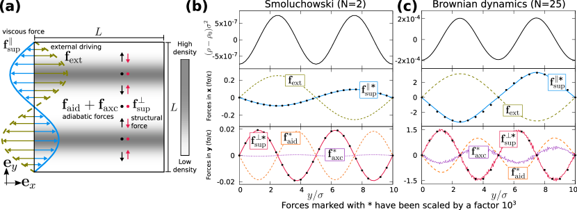
Figure 1: (a) Illustration of the setup of a sinusoidal inhomogeneous shear flow induced by the external force field (9). Shown are the superadiabatic viscous force, which opposes the externally induced flow, the adiabatic excess and ideal forces, which tend to relax the density gradient, as well as the superadiabatic structural nonequilibrium force, which restores the force balance in the $y$-direction. (b) Steady-state density and force profiles obtained by numerically solving the Smoluchowski equation in a system with $N=2$, $L/\sigma=10$, and $k_{B}T/\epsilon=0.4$. (Top panel) Density profile for average density $\rho_{0}=N/L^{2}=0.02\sigma^{-2}$ as a function of $y$. (Middle panel) Forces acting along ${\bf e}_{x}$ as a function of $y$: external force ${\bf f}_{\rm ext}$ of imposed amplitude $f_{0}\approx 0.25\epsilon/\sigma$ (green-dashed line), and superadiabatic viscous force (solid-blue line) ${\bf f}_{\rm sup}^{\parallel}$. (Bottom panel) Forces acting along ${\bf e}_{y}$ as a function of $y$: adiabatic ideal (diffusion) ${\bf f}_{\rm aid}$ (orange dashed line), adiabatic excess ${\bf f}_{\rm axc}$ (violet dotted line), and superadiabatic structural force ${\bf f}_{\rm sup}^{\perp}$ (solid-red line). (c) Same as (b) but for a system with $N=25$, $L/\sigma=10$, $\rho_{0}=0.25\sigma^{-2}$, $k_{B}T/\epsilon=1$ and $f_{0}\approx 3.14\epsilon/\sigma$. Data obtained using BD simulations. Forces marked with an asterisk in (b) and (c) have been multiplied by $10^{3}$ for clarity. The black circles in panels (b) and (c) indicate the theoretical prediction (18) of the superadiabatic viscous and structural forces.

In order to study the system on the Fokker-Planck level, we solve numerically the exact many-body Smoluchowski equation (SE) for overdamped Brownian motion. The time evolution of the probability distribution $\Psi$ is given exactly by the many body continuity equation

$$\frac{\partial\Psi({\mathbf{r}}^{N},t)}{\partial t}=-\sum_{i}\nabla_{i}\cdot{\bf v}_{i}\Psi({\mathbf{r}}^{N},t).$$ (10)

where ${\bf v}_{i}$ is the velocity of particle $i$, given by the force balance

$$\gamma{\bf v}_{i} =-\nabla_{i}(u({\mathbf{r}}^{N})+k_{B}T\ln\Psi({\mathbf{r}}^{N},t))+{\bf f}_{\rm ext}({\mathbf{r}}_{i},t).$$ (11)

We solve (10) and (11) numerically using a (standard) operator splitting approach NumericalRecipes . Each spatial coordinate is discretized in increments $\Delta x=\sigma/5$; we use a time step $\Delta t/\tau=5\times 10^{-3}$ with timescale $\tau=\sigma^{2}\gamma/\epsilon$. This method provides exact results of the nonequilibrium dynamics up to numerical inaccuracies. For $d$ space dimensions, the dimension of configuration space is $Nd$, which limits the applicability of the method to systems with small numbers of particles. Here, we consider $N=2$ in $d=2$, which renders the numerical field $Nd=4$ dimensional; hence including time, we solve a $4+1$ dimensional numerical problem. As we show, despite the limited number of particles, all relevant forces are present.

In order to analyse larger systems, we use Brownian dynamics (BD), i.e. integrating in time the Langevin equation of motion, which corresponds to (10) and (11):

$$\gamma\frac{d{\mathbf{r}}_{i}(t)}{dt} =-\nabla_{i}u({\mathbf{r}}^{N})+{\bf f}_{\rm ext}({\mathbf{r}}_{i},t)+\boldsymbol{\chi}_{i}(t),$$ (12)

where $\boldsymbol{\chi}_{i}$ is a delta-correlated Gaussian random force. We use a time step $dt/\tau=10^{-4}$ and histogram bins of size $\Delta x=\sigma/20$. Density and force density profiles are obtained by averaging over a total time of $\sim 10^{9}\tau$ in steady state.

In both SE and BD we use the iterative scheme of Refs. fortini14prl ; bernreuther16pre to construct the adiabatic external potential $V_{{\rm ad},t}({\mathbf{r}})$. The superadiabatic force then follows immediately from (5) since both ${\bf f}_{\rm int}$ and ${\bf f}_{\rm axc}$ can be directly calculated (sampled) in SE (BD). We have used the recently developed force sampling method delasHeras2017sampling to improve the sampling of the density profile in BD. We expect, on principal grounds, that the SE and BD results agree (for identical values of system size and particle number, here $N=2$).

A schematic showing all forces in steady state is shown in Fig. 1a. The stationary density- and force-profiles obtained by solving the Smoluchowski equation $(N=2)$, and using BD simulations $(N=25)$ are shown in Fig. 1b and Fig. 1c, respectively. A net flow exists along $+{\bf e}_{x}$, since the external force is only partially balanced by a superadiabatic force of viscous nature, ${\bf f}_{\rm sup}^{\parallel}$, along $-{\bf e}_{x}$ (see middle panels). Hence in this situation ${\mathbf{e}}_{v}={\mathbf{e}}_{x}$. The viscous force has roughly the same shape as the external force but with reversed direction. The inhomogeneous external force (9), ${\bf f}_{\rm ext}(y)$, creates a density gradient in ${\bf e}_{y}$ (see top panels), since the particles migrate to the low shear rate regions. The adiabatic ideal (i.e. diffusive) and adiabatic excess (i.e. due to internal interaction) forces act along ${\bf e}_{y}$ and both try to relax the density gradient (see bottom panels). Both adiabatic forces are, however, exactly balanced by a structural superadiabatic force ${\bf f}_{\rm sup}^{\perp}$. The presence of the structural force hence renders the inhomogeneities of the density profile stationary in time.

We next analyse the system more systematically by comparing the behaviour of the structural force to that of the viscous force. We show in Fig. 2a the amplitudes of the viscous force, $\hat{f}_{\rm sup}^{\parallel}$, and the structural force, $\hat{f}_{\rm sup}^{\perp}$, (measured from maximum to baseline) as a function of the amplitude of the external driving, $f_{0}$. For small driving the viscous force scales linearly with $f_{0}$. This behaviour is expected, since for weak driving the velocity is proportional to the strength of the driving and the viscous force is proportional to the velocity (Newtonian rheology). The structural force, on the other hand, scales quadratically with $f_{0}$ and hence also with the velocity in the small driving regime. Both forces saturate for high values of $f_{0}$, see the inset in Fig. 2a. Fig. 2b shows $\hat{f}_{\rm sup}^{\parallel}$ and $\hat{f}_{\rm sup}^{\perp}$ as a function of the average density $\rho_{0}$, revealing again profound differences between viscous and structural forces. The viscous force increases linearly with increasing $\rho_{0}$ at low densities and it saturates at high densities. In contrast, the structural force is non-monotonic and exhibits a maximum at an intermediate density.

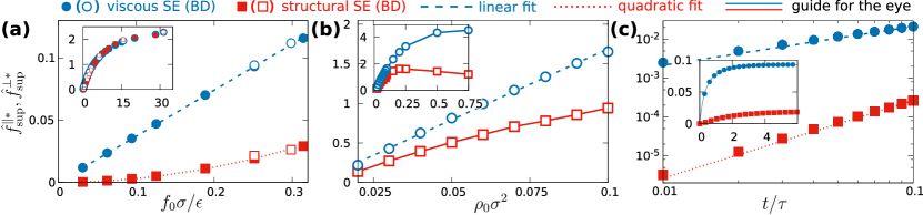
Figure 2: Scaled amplitude of the superadiabatic forces $\hat{f}_{\rm sup}^{\alpha*}=10^{3}\hat{f}_{\rm sup}^{\alpha}\sigma/\epsilon$ with $\alpha\in\{\parallel,\perp\}$, as a function of: (a) the amplitude of the external driving force $f_{0}$, (b) the average density $\rho_{0}=N/L^{2}$, and (c) the time $t$. (a) Results for $L/\sigma=10$, $N=2$, and $k_{B}T/\epsilon=0.4$. (b) Results in a system with $L/\sigma=10$, $f_{0}\approx 3.14\epsilon/\sigma$, $k_{B}T/\epsilon=1$ and varying $N$. (c) Note the logarithmic scale in the main plot. The external driving force is switched on at $t=0$. Results for $L/\sigma=10$, $N=2$, $k_{B}T/\epsilon=0.4$, and $f_{0}\approx 0.25\epsilon/\sigma$. In all panels, the viscous (structural) superadiabatic force is represented with blue circles (red squares), as indicated in the upper legend. Full (empty) symbols correspond to SE (BD) calculations. The blue dashed (red dotted) line indicates a linear (quadratic) fit to the data, as detailed in the SupMat . Solid lines are guides to the eye. The inset in each figure shows a linear plot of the same quantities as those in the main plot, but over an extended region.

We rationalize these findings by developing a theory within the power functional approach power . Here the adiabatic and the superadiabatic contributions to the internal force field (5) are obtained via functional differentiation of two generating functionals:

$${\bf f}_{\rm axc}({\mathbf{r}},t) =-\nabla\frac{\delta F_{\rm exc}[\rho]}{\delta\rho({\mathbf{r}},t)},$$ (13)

$${\bf f}_{\rm sup}({\mathbf{r}},t) =-\frac{\delta P_{t}^{\rm exc}[\rho,{\bf J}]}{\delta{\bf J}({\mathbf{r}},t)}.$$ (14)

Here $F_{\rm exc}[\rho]$ is the intrinsic excess (over ideal) Helmholtz equilibrium free energy functional of density functional theory, and $P_{t}^{\rm exc}[\rho,{\bf J}]$ is the excess (again over ideal) superadiabatic functional of power functional theory power . Dynamical density functional theory (DDFT) evans79 ; marinibettolomarconi99 ; archer04ddft is obtained by setting $P_{t}^{\rm exc}=0$; hence no superadiabatic forces (neither viscous nor structural) occur in DDFT. In Ref. delasHeras17gradvel , using a change of variables in power functional theory from the current ${\bf J}$ to the velocity gradient $\nabla{\bf v}$, it is shown that the excess superadiabatic functional can be represented as a functional of $\nabla{\bf v}$. Following the same line, we consider a temporally non-Markovian, but spatially local form:

$$P_{t}^{\rm exc} =\int d{\mathbf{r}}\Big{[}\int_{0}^{t}dt^{\prime}n_{tt^{\prime}}(\nabla\times{\bf v})\cdot(\nabla\times{\bf v}^{\prime})$$ (15)

$$\quad-\int_{0}^{t}dt^{\prime}\int_{0}^{t}dt^{\prime\prime}m_{tt^{\prime}t^{\prime\prime}}(\nabla\cdot{\bf v})(\nabla\times{\bf v}^{\prime})\cdot(\nabla\times{\bf v}^{\prime\prime})\Big{]},$$

where we have used the short-hand notation ${\bf v}^{\prime}={\bf v}({\mathbf{r}},t^{\prime})$ and ${\bf v}^{\prime\prime}={\bf v}({\mathbf{r}},t^{\prime\prime})$. The factors $n_{tt^{\prime}}$ and $m_{tt^{\prime}t^{\prime\prime}}$ are density-dependent temporal convolution kernels; the subscripts indicate the time arguments; here the dependence is on the differences $t-t^{\prime}$ and $t-t^{\prime\prime}$; the specific form of the kernels will depend on the form of the interparticle interaction potential $u({\mathbf{r}}^{N})$. In (15) we have left away bi-linear and higher contributions in $\nabla\cdot{\bf v}$ delasHeras17gradvel ; these are important for compressional flow, but not for the present shear setup. Furthermore, as $\rho$ is practically constant in the cases considered, contributions in $\nabla\rho$ have also been omitted.

The superadiabatic force field is then obtained by inserting (15) into (14), where the derivative is carried out at fixed density, and hence $\delta/\delta{\bf J}=\rho^{-1}\delta/\delta{\bf v}$. Furthermore the spatial derivatives in (15) can be suitably re-arranged by (spatial) integration by parts. The resulting force density is

$$\rho{\bf f}_{\rm sup}({\mathbf{r}},t) =\int_{0}^{t}dt^{\prime}\nabla\cdot n_{tt^{\prime}}\nabla{\bf v}^{\prime}$$ (16)

$$\quad-\int_{0}^{t}dt^{\prime}\int_{0}^{t}dt^{\prime\prime}\nabla m_{tt^{\prime}t^{\prime\prime}}(\nabla\times{\bf v}^{\prime})\cdot(\nabla\times{\bf v}^{\prime\prime}).$$

In steady state and for the case of constant density profile, (16) reduces to:

$$\rho{\bf f}_{\rm sup}({\mathbf{r}}) =\eta\nabla^{2}{\bf v}-\chi\nabla(\nabla\times{\bf v})^{2},$$ (17)

where the prefactors $\eta=\lim_{t\to\infty}\int_{0}^{t}dt^{\prime}n_{tt^{\prime}}$ and $\chi=\lim_{t\to\infty}\int_{0}^{t}dt^{\prime}\int_{0}^{t}dt^{\prime\prime}m_{tt^{\prime}t^{\prime\prime}}$ are moments of the convolution kernels, which depend on the overall density. We can identify $\eta$ with the shear viscosity delasHeras17gradvel , such that the first term in (17) represents the viscous force. From carrying out the normal projection (8), the second contribution in (17) yields the structural force ${\bf f}_{\rm sup}^{\perp}({\mathbf{r}},t)$. Note that while the forms (16) and (17) could possibly be postulated based on symmetry considerations alone, in the current framework, the generator (15) constitutes the more fundamental object, as the form of the force field follows via the functional derivative (14). Note that for the ideal gas ($u=0$) $P_{t}^{\rm exc}=0$ and ${\bf f}_{\rm sup}$=0 by construction power .

In accordance with our numerical results, we assume that the flow field is dominated by the external force, hence we approximate (1) by ${\bf v}(y,t)\approx{\bf f}_{\rm ext}(y,t)/\gamma$. Insertion of (9) into (17) then yields

$${\bf f}_{\rm sup}(y) =-\frac{f_{0}\eta k^{2}}{\gamma\rho}\sin(ky){\mathbf{e}}_{x}+\frac{f_{0}^{2}\chi k^{3}}{\gamma\rho}\sin(2ky){\mathbf{e}}_{y},$$ (18)

where $k=2\pi/L$. In Fig. 1b and 1c we show the comparison between the predicted (black circles) and the computed superadiabatic forces using SE and BD (solid lines). The values of the response coefficients $\eta$ and $\chi$, cf. (18), have been adjusted to fit each amplitude, see SupMat for details.

The theory then predicts the shape of both viscous and structural forces without further adjustable parameters, and it is in excellent agreement with the results from SE and BD. In addition, the linear (quadratic) scaling of the viscous (structural) force with the velocity, Fig. 2a, is also accounted by the theory, cf. (17). Due to the saturation of both superadiabatic forces (inset of Fig. 2a) it is necessary to analyze very small driving to obtain the correct scaling. Also, at low average density $\rho_{0}$ the viscous force is proportional to $\rho_{0}$ (see Fig. 2b), which according to (18) implies $\eta\propto\rho_{0}^{2}$, as expected reinhardt2013 . See SupMat for results for strong driving conditions and for a theoretical prediction of the density profile.

Memory plays a vital role in nonequilibrium systems, as we show in Fig. 2c by investigating the transient time evolution after switching on the driving at $t=0$, cf. (9). Both superadiabatic force contributions vanish in equilibrium ($t\leq 0$) and saturate in steady state ($t\rightarrow\infty$). At short times after switching on the driving force, the viscous (structural) force is linear (quadratic) in $t$, in full agreement with the non-Markovian form of (15). See SupMat for an analysis of the scaling of the amplitude of the forces with wavenumber $k$. Here we have still taken ${\mathbf{e}}_{v}={\mathbf{e}}_{x}$ as a (very good) approximation.

We conclude that the structural force is a primary candidate for a universal mechanism that leads to nonequilibrium structure formation. Examples of systems where a force acts perpendicular to the flow include shear banding dhont1999 ; dhont2003 ; dhont2014 , colloidal lane formation laningLitOne ; laningLitTwo , and effective interactions in active spinning particles ActiveRotPRL ; aragonesNC . The theory that we present here operates in a self-contained way on the one-body level of correlation functions, and hence is different from the approach of Refs. braderkrueger11molphys ; scacchi2016 , where a dynamic closure on the two-body level via modelling of Brownian “scattering” is postulated. Note that the treatment of Refs. braderkrueger11molphys ; scacchi2016 relies on the density distribution as the fundamental variable; in contrast, our theory, predicts the behaviour of the system directly from the velocity field, cf. (16) and (17).

We have focused here on the viscous and the structural contributions to the superadiabatic force in shear-type flow. In compressional flow, where $\nabla\cdot{\bf v}\neq 0$, further force contributions can occur. Calculating the values for the transport coefficients $\eta$ and $\chi$ within the current theory is desirable, based, e.g., on the two-body level of correlation functions NOZ . Furthermore, interesting research task for the the future include investigating the effects of inhomogeneous temperature fields falasco2016 , and the possible emergence of time-periodic states (“time crystals”timeCrystals ) in inertial dynamics inertialPFT .

This work is supported by the German Research Foundation (DFG) via SCHM 2632/1-1. N. C. X. S. and T. E. contributed equally to this work.

I Supplemental Material: Structural nonequilibrium forces in driven colloidal systems

I.1 Superadiabatic force profiles under strong driving conditions

The examples presented in the main text address the behaviour of the system in response to relatively weak external perturbations. Here we show that under strong external driving conditions, both superadiabatic force profiles change significantly. We show in Supplemental Fig. 3 the viscous and the structural superadiabatic forces for both weak and for strong external driving conditions. We find that the direction of both force fields remains unchanged upon increasing the driving. Hence, for the cases considered here, the viscous force opposes always the external force and the structural force sustains (counteracts) the density gradient. However, although the only difference between both driving conditions is the magnitude of the external driving, the superadiabatic (position-dependent) force profiles change significantly their shape depending on the strength of the driving. The power functional approximation presented in Eq. (15) of the main text is intended to deal with low/moderate driving and does not fully reproduce the characteristics of the superadiabatic forces at high driving conditions. Note that the magnitude of the superadiabatic force is relatively small as compared to the magnitude of the external force, even for the case of weak driving (Fig. 1 of the main text). Therefore, the velocity field basically follows the external driving, and the superadiabatic forces are then given by Eq. (18) of the main text. That is, the theory does not reproduce the shape change of the superadiabatic forces with the magnitude of the external driving (Supplemental Fig. 3). This was expected since in Eq. (15) we have only incorporated the first two terms of the expansion of $P_{t}^{\text{exc}}$ in powers of $\nabla{\bf v}$. Therefore, one expects Eq. (15) to be valid under weak driving conditions. The correct treatment of strong driving conditions requires the addition of higher order terms to Eq. (15). It is straightforward to incorporate such terms by rewriting the excess superadiabatic functional as

$$P^{\rm exc} =\int d{\mathbf{r}}\Big{[}\eta(\nabla\!\times\!{\bf v})^{2}-\chi(\nabla\!\cdot\!{\bf v})(\nabla\!\times\!{\bf v})^{2}\Big{]}h(\nabla{\bf v}),$$ (19)

where $h(\nabla{\bf v})$ is a scalar-valued function, which we choose to have the following form:

$$h(\nabla{\bf v})=\frac{1}{1+c_{0}(\nabla\times{\bf v})^{2}},$$ (20)

where $c_{0}$ is a positive constant which controls the strength of the influence of the flow; setting $c_{0}=0$ recovers the form of Eq. (15) of the main text. In Eq. (19) we have assumed steady state conditions and therefore eliminated the time integrals. The first two terms of a series expansion of Eq. (19) in $\nabla{\bf v}$ have the same functional structure as that presented in Eq. (15) of the main text. In addition, Eq. (19) incorporates higher order contributions in $\nabla{\bf v}$. We find that the superadiabatic force profile that result upon functional differentiation of Eq. (19) is in excellent agreement with the simulation results both for weak and for strong driving conditions (see black circles in Supplemental Fig. 3). For both cases shown in the figure, we have set $c_{0}=3.5\cdot 10^{-3}\;\;\tau^{2}$ and fit the values of $\eta$ and $\chi$. The values of $\eta$ and of $\chi$ determine the overall amplitude of the viscous and of the structural superadiabatic force, respectively. We find that the values of $\eta$ and $\chi$ seem to depend on the magnitude of the external driving, which is a clear indication that Eq. (19) constitutes only a first approximation.

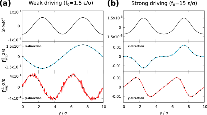
Figure 3: Steady-state density and force profiles according to BD simulations in a system with $N=25$, $L/\sigma=10$, and $k_{B}T/\epsilon=1.0$. Results are shown for two strengths of the external driving force: (a) $f_{0}\approx 1.5\epsilon/\sigma$, weak external driving, and (b) $f_{0}\approx 15\epsilon/\sigma$, strong external driving. (Top panels) Density profile, measured from the average density $\rho_{0}=N/L^{2}=0.25\sigma^{-2}$, as a function of $y$. (Middle panel) Superadiabatic viscous force acting along ${\bf e}_{x}$ as a function of $y$ obtained by BD simulations (solid-blue line) and theoretically (black circles). (Bottom panel) Superadiabatic structural force acting along ${\bf e}_{y}$ as a function of $y$ obtained by BD simulations (solid-red line) and theoretically (black circles).

I.2 Scaling of the superadiabatic forces with the inverse box length

We present a scaling analysis of the magnitude of the viscous and of the structural superadiabatic force fields with the amplitude of the external driving and the overall density in the main text. Here, we focus on the scaling of these force fields with the wavenumber $k=2\pi/L$ that characterizes the inhomogeneous shear profile, cf. Eq. (9) of the main text. In practice we change $k$ by changing the box size $L$, ensuring that the other relevant variables are unchanged, e.g. keeping the mean density constant by accordingly modifying the number of particles, $N$.

Our theory, cf. Eq. (18) of the main text, predicts different types of scaling with $k$ for the viscous (quadratic in $k$) and for the structural (cubic in $k$) superadiabatic forces. We fix the amplitude of the external driving ($f_{0}\approx 0.30\epsilon/\sigma$) and the average density of the system ($\rho_{0}\sigma^{2}=0.02$). Therefore, according to Eq. (18) of the main text, the only remaining dependence of the amplitude of the superadiabatic forces is on $k$. In Supplemental Fig. 4 we show the amplitude of the superadiabatic forces as a function of the wavenumber. The smallest system corresponds to $N=2$ and $H/\sigma=10$, and the largest one to $N=100$ and $H/\sigma=70.7$. Each curve shows three different regimes. For small boxes (large wavenumber) we observe a saturation of the superadiabatic forces, similar to the saturation effect observed by increasing the external driving or the density (see Fig. 2 of the main text). At intermediate wavenumbers the forces scale linearly with $k$. Finally, for long boxes (small wavenumbers) the curves depart significantly from a linear behaviour. Note that both curves must pass through the origin of coordinates. The low driving conditions that are implicit in going to small values of $k$ render the analysis of the data difficult. Nevertheless, the scaling of the viscous force is fully consistent with the quadratic prediction of the theory, Eq. (18) of the main text. Also, it is evident from the data that the structural force is not linear in $k$ for sufficiently large boxes (small wavenumbers). The precision of our data, however, does not allow us to confirm the cubic scaling predicted by the theory, although the data is also clearly not in contradiction to the analytical result. We hence cannot rule out the contribution of further terms to $P_{t}^{\rm exc}$. In particular, a term involving the combination $(\nabla\cdot{\bf v})({\bf v}\cdot{\bf v})$ produces a structural force with the same shape, but a linear scaling with $k$. We conclude that revealing the true scaling of the superadiabatic forces is a major challenge. Due to the saturation effect, the forces increase linearly in a broad range of system sizes. Only for very small perturbations (very large system sizes in this case) the true scaling behaviour is revealed.

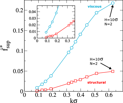
Figure 4: Scaled amplitude of the superadiabatic forces $\hat{f}_{\rm sup}^{*}=10^{3}\hat{f}_{\rm sup}\sigma/\epsilon$ as a function of the (scaled) wavenumber $k\sigma=2\pi\sigma/L$. The blue circles (red squares) correspond to the viscous (structural) superadiabatic force, as indicated. The lines are guides to the eye. Data obtained with BD simulations for systems with $k_{B}T/\epsilon=0.4$ and $f_{0}\approx 0.30\epsilon/\sigma$. The number of particles and the length of the box vary across the data points, such that the average density $\rho_{0}\sigma^{2}=0.02$ is kept constant. Both curves must pass through the origin.

I.3 Representation of numerical results via fit functions

The fit parameters in Fig. 2a of the main text are: $A_{1}=3.7\cdot 10^{-4}$ (for the viscous force, linear in velocity), $A_{2}=3.0\cdot 10^{-5}\sigma/\epsilon$ (for the structural force, quadratic in velocity). The fit has been done in the region of weak driving $f_{0}\sigma/\epsilon\lesssim 0.3$.

Regarding the scaling of the superadiabatic forces with the total density, Fig. 2b of the main text ($f_{0}\approx 3.14\epsilon/\sigma)$, a good numerical representation in the range $0<\rho_{0}\sigma^{2}<0.1$ is given by $\eta(\rho_{0})\approx 1.7\cdot 10^{-2}\rho_{0}^{2}\epsilon\tau\sigma^{2}$ and $\chi(\rho_{0})\approx 10^{-2}\rho_{0}^{2}\epsilon\tau^{2}\sigma^{2}-0.4\cdot 10^{-2}\rho_{0}^{3}\epsilon\tau^{2}\sigma^{4}$.

We reemphasize that the true scaling of viscous and structural forces is only revealed at weak driving conditions and low densities. At intermediate driving and/or total density both forces are linear in velocity and total density due to a, yet to be investigated, saturation mechanism of the superadiabatic forces.

I.4 Predicting the density profile

We can obtain a prediction of the density profile from the theory, by projecting the force balance equation (Eq. (1) of the main text) onto ${\mathbf{e}}_{y}$ and observing that ${\bf v}\cdot{\mathbf{e}}_{y}=0={\bf f}_{\rm ext}\cdot{\mathbf{e}}_{y}$. We obtain $k_{B}T\partial\rho/\partial y=f_{\rm sup,y}$ upon neglecting the adiabatic excess contribution ${\bf f}_{\rm adx}$, as this is small against the ideal term, $|{\bf f}_{\rm adx}|\ll|k_{B}T\nabla\rho|$ in the low density case $N=2$. Integrating in $y$ gives to lowest order in the difference $\rho-\rho_{0}$ the result $\rho(y)=\rho_{0}-f_{0}^{2}\chi k^{2}\cos(2ky)/(2\gamma k_{B}T)$, which describes the low-density case (Fig. 3b of the main text) quite well.

References

- (1) J. K. G. Dhont, Phys. Rev. E 60, 4534 (1999).
- (2) J. K. G. Dhont et.al, Faraday Discuss. 123, 157 (2003).
- (3) H. Jin, K. H. Ahn and J. K. G. Dhont, Soft Matter 10, 9470 (2014).
- (4) J. Chakrabarti, J. Dzubiella, and H. Löwen, Phys. Rev. E 70, 012401 (2004).
- (5) C. W. Wächtler, F. Kogler, and S. H. L. Klapp, Phys. Rev. E 94, 052603 (2016).
- (6) M. Krüger and and J. M. Brader EPL 96, 68006 (2011).
- (7) J. M. Brader and M. Krüger, Mol. Phys. 109, 1029 (2011).
- (8) J. Reinhardt, F. Weysser and J. M. Brader, EPL 102, 28011 (2013).
- (9) A. A. Aerov and M. Krüger, J. Chem. Phys. 140, 094701 (2014).
- (10) A. A. Aerov and M. Krüger, Phys. Rev. E 92, 042301 (2015).
- (11) A. Scacchi, M. Krüger and J. M. Brader, J. Phys.: Condens. Matter 28, 244023 (2016).
- (12) J. Zausch, J. Horbach, M. Laurati, S. U. Egelhaaf, J. M. Brader, Th. Voigtmann, and M. Fuchs, J. Phys.: Condens. Matter 20, 404210 (2008).
- (13) Ch. J. Harrer, D. Winter, J. Horbach, M. Fuchs and Th. Voigtmann, J. Phys.: Condens. Matter 24, 464105 (2012).
- (14) R. Ni, S. Cohen, A. Martien P. G. Bolhuis, Phys. Rev. Lett. 114, 018302 (2015).
- (15) U. Zimmermann, F. Smallenburg and H. Löwen, J. Phys.: Condens. Matter 28, 244019 (2016).
- (16) D. de las Heras, N. Doshi, T. Cosgrove, J. Phipps, D. I. Gittins, J. S. van Duijneveldt and M. Schmidt, Sci. Rep. 2, 789 (2012).
- (17) B. Ruzicka, E. Zaccarelli, L. Zulian, R. Angelini, M. Sztucki, A. Moussaïd, T. Narayanan and F. Sciortino, Nat. Mater. 10, 56 (2011).
- (18) M. Schmidt and J. M. Brader, J. Chem. Phys. 138, 214101 (2013).
- (19) A. Fortini, D. de las Heras, J. M. Brader, M. Schmidt, Phys. Rev. Lett. 113, 167801 (2014).
- (20) D. de las Heras and M. Schmidt, Phys. Rev. Lett. 120, 028001 (2018).
- (21) see, e.g., A.J Archer and R. Evans, Phys. Rev. E 64, 041501 (2001); A.J. Archer, J. Phys.: Condens. Matter 17 1405 (2005).
- (22) W. H. Press, S. A. Teukolsky, W. T. Vetterling, and B. P. Flannery, Numerical Recipes: The Art Of Scientific Computing, 3rd ed. (Cambridge University Press, Cambridge, 2007).
- (23) E. Bernreuther and M. Schmidt, Phys. Rev. E 94, 022105 (2016).
- (24) D. de las Heras and M. Schmidt, Phys. Rev. Lett. 120, 218001 (2018).
- (25) R. Evans, Adv. Phys. 28, 143 (1979).
- (26) U. Marini Bettolo Marconi and P. Tarazona, J. Chem. Phys. 110, 8032 (1999).
- (27) A. J. Archer and R. Evans, J. Chem. Phys. 121, 4246 (2004).
- (28) See Supplemental Material for descriptions of: superadiabatic force profiles under strong driving conditions, scaling of the superadiabatic forces with the inverse box length, fitting details, and theoretical prediction of the density profile.
- (29) N. H. P. Nguyen, D. Klotsa, M. Engel and S. C. Glotzer, Phys. Rev. Lett. 112, 075701 (2014).
- (30) J. L. Aragones, J. P. Steimel and A. Alexander-Katz, Nat. Commun. 7, 11325 (2016).
- (31) J. M. Brader, M. Schmidt, J. Chem. Phys. 139, 104108 (2013); J. Chem. Phys. 140, 034104 (2014); J. Phys.: Condens. Matter 27, 194106 (2015).
- (32) For recent work, see e.g., G. Falasco and K. Kroy, Phys. Rev. E 93, 032150 (2016).
- (33) J. Zhang et al, Nature 543, 217 (2017); R. Moessner and S. L. Sondhi, Nat. Phys. 13, 424 (2017).
- (34) Power functional theory for quantum and for classical Newtonian dynamics is formulated, respectively, in: M. Schmidt, J. Chem. Phys. 143, 174108 (2015); J. Chem. Phys. 148, 044502 (2018).