Expected Chromatic Number of Random Subgraphs

Abstract

Given a graph $G$ and $p\in[0,1]$, let $G_{p}$ denote the random subgraph of $G$ obtained by keeping each edge independently with probability $p$. Alon, Krivelevich, and Sudokov [2] proved $\mathbb{E}[\chi(G_{p})]\geq C_{p}\frac{\chi(G)}{\log|V(G)|}$, and Bukh [6] conjectured an improvement of $\mathbb{E}[\chi(G_{p})]\geq C_{p}\frac{\chi(G)}{\log\chi(G)}$. We prove a new spectral lower bound on $\mathbb{E}[\chi(G_{p})]$, as progress towards Bukh’s conjecture. We also propose the stronger conjecture that for any fixed $p\leq 1/2$, among all graphs of fixed chromatic number, $\mathbb{E}[\chi(G_{p})]$ is minimized by the complete graph. We prove this stronger conjecture when $G$ is planar or $\chi(G)<4$. We also consider weaker lower bounds on $\mathbb{E}[\chi(G_{p})]$ proposed in a recent paper by Shinkar  [17]; we answer two open questions posed in [17] negatively and propose a possible refinement of one of them.

1 Introduction

For a graph $G$ and $p\in[0,1]$, we obtain a probability distribution $G_{p}$ called a random subgraph by taking subgraphs of $G$ with each edge appearing independently with probability $p$. When $G=K_{n}$ is the complete graph on $n$ vertices, this is called the Erdős–Rényi random graph, denoted $G(n,p)$. A proper coloring of a graph is an assignment of colors to the vertices such that no two adjacent vertices are the same color. Finally, the chromatic number $\chi(G)$ of a graph is the minimal number of colors needed to construct a proper coloring.

The chromatic number is one of the most important parameters of a graph, and many problems in computer science—e.g., register allocation, pattern matching, and scheduling problems—can be reduced to finding the chromatic number of a given graph. In the probabilistic setting, the distribution of $\chi(G_{p})$ is studied in statistical mechanics, where physicists use random subgraphs to model molecular interactions, and properties of the resulting graph colorings are predictive of various macroscopic features  [4].

The chromatic number of the Erdős–Rényi graph has been particularly well studied, and (for $p$ constant) Bollobás [5] was able to show that $\mathbb{E}[\chi(G(n,p))]\sim c_{p}\cdot n/\log{n}=c_{p}\chi(K_{n})/\log{\chi(K_{n})}$, where $c_{p}$ is a constant depending on $p$, and the notation $A\sim B$ is used to mean that $A/B$ tends to $1$ as the relevant parameter (here $n$) tends to infinity. For general graphs, one cannot hope for such tight control over $\chi(G_{p})$ only in terms of $\chi(G)$. The trivial upper bound $\chi(G_{p})\leq\chi(G)$ is asymptotically best possible when $G$ is a disjoint union of many cliques, and the first general lower bound was was given by Alon, Krivelevich, and Sudakov [2], who proved $\chi(G_{1/2})\geq\frac{\chi(G)}{2\log_{2}|V(G)|}$ almost surely (i.e., with probability tending to $1$). However, this ceases to be a meaningful bound when $|V(G)|\gg\chi(G)$, and Bukh  [6] asks whether it can be improved by eliminating the dependence on $|V(G)|$.

Question 1 (Bukh).

For each $p\in[0,1]$, is there a constant $c_{p}>0$ such that $\mathbb{E}[\chi(G_{p})]>c_{p}\cdot\frac{\chi(G)}{\log\chi(G)}$ for all graphs $G$?

Thus, in light of Bollobás’s result, Bukh asks whether $\mathbb{E}[\chi(G_{p})]$ is (up to a constant) minimized by $G=K_{n}$.

While this question is still unresolved, several papers have made progress towards an affirmative answer. In addition to providing concentration results on $\chi(G_{p})$, Shinkar [17] proved that if $|V(G)|=n$, then

$$\mathbb{E}[n/\alpha(G_{p})]\geq C_{p}\frac{n/\alpha(G)}{\log{(n/\alpha(G))}},$$ (1.1)

where $\alpha(H)$ denotes the independence number of $H$ (i.e., the maximum size of a set of vertices containing no edges), and Mohar  [14] proved an affirmative analog to Bukh’s question when each instance of $\chi$ is replaced by the fractional chromatic number, $\chi_{f}$. Though incomparable, these results are related by the general fact that $|V(H)|/\alpha(H)\leq\chi_{f}(H)\leq\chi(H)$ for all $H$. Thus, these affirmatively resolve question 1 for any graph for which $n/\alpha(G)$ (or somewhat more generally $\chi_{f}(G)$) is within a multiplicative factor of $\chi(G)$, which by [5] includes almost all graphs. The only other general lower bound on $\chi(G_{p})$ is a short coupling argument in [17] showing $\mathbb{E}[\chi(G_{1/m})]\geq\chi(G)^{1/m}$ for all positive integers $m$.

As one of the main results of this paper, we use recent developments from random matrix theory and a celebrated result of Hoffman [11] to obtain a new spectral lower bound on $\mathbb{E}[\chi(G_{p})]$. Recalling relevant definitions, for a graph $H$ its adjacency matrix is the matrix indexed by $V(H)$ whose $(u,v)$-entry is $1$ if $u\sim v$ and $0$ otherwise. Because this matrix is real-symmetric, all its eigenvalues are real, and we may define $\lambda_{\textup{min}}(H)$ and $\lambda_{\textup{max}}(H)$ to be its least and greatest eigenvalues (respectively). We prove the following.

Theorem 1.

There is a constant $C>0$ such that for each $p\in(0,1)$, for any graph with maximum degree $\Delta$ and $n=|V(G)|$, we almost surely have

$$\frac{\lambda_{\textup{max}}(G_{p})}{-\lambda_{\textup{min}}(G_{p})}\geq\frac{\lambda_{\textup{max}}(G)-(C/p)(\sqrt{\Delta}+\sqrt{\log(n)})}{-\lambda_{\textup{min}}(G)+(C/p)(\sqrt{\Delta}+\sqrt{\log(n)})}.$$

In particular, almost surely $\chi(G_{p})\geq\frac{\lambda_{\textup{max}}(G)}{-\lambda_{\textup{min}}(G)+(C/p)(\sqrt{\Delta}+\sqrt{\log(n)})}.$

The second part of the above follows from Hoffman’s result that $n/\alpha(H)\geq 1+\frac{\lambda_{\textup{max}}(H)}{-\lambda_{\textup{min}}(H)}$, which gives an affirmative answer to question 1 provided essentially that Hoffman’s bound differs from $\chi(G)$ by at most a factor of $\log\chi(G)$ and that $-\lambda_{\textup{min}}(G)$ is not much less than $\sqrt{\Delta}+\sqrt{\log(n)}$. For instance, we show that there is an infinite family of graphs—namely appropriately chosen Kneser graphs—for which our spectral bound implies Bukh’s bound, while none of the other general bounds on $\mathbb{E}[\chi(G_{p})]$ are able to. (Although for Kneser graphs, the behavior of $\alpha(G_{p})$ and $\chi(G_{p})$ is already well-understood [7, 12].)

In addition to this spectral bound, we also propose and study the following two conjectures, which are readily seen as weaker and stronger (resp.) than an affirmative answer to question 1.

Conjecture 1.

For each $p\in[0,1]$, there is a constant $c_{p}$ such that $\mathbb{E}[\chi(G_{p})]\geq c_{p}\cdot\chi(G)^{p}$ for all $G$.

Conjecture 2.

For each $p\leq\frac{1}{2}$, we have $\mathbb{E}[\chi(G_{p})]\geq\mathbb{E}[\chi(G(n,p))]$ for all $G$ with $\chi(G)=n$.

Conjecture 1 was originally posed in [17] with the constant $c_{p}=1$; however, we show that in general $c_{p}<1$ is in fact required. As discussed in section 3, in the case $p=1/m$, a proof of this conjecture (with $c_{p}=1$) follows from the classic result of Zykov [16] that $\chi(G\cup H)\leq\chi(G)\chi(H)$. However, the tightness in our following generalization of this result highlights a barrier to this approach for general $p$.

Theorem 2.

Fix integers $0\leq t<n$. Let $G$ be a graph and $G_{1},G_{2},\dots,G_{n}\subset G$ such that every edge of $G$ lies in at least $n-t$ of the $G_{i}$. Then $\chi(G_{1})\chi(G_{2})\cdots\chi(G_{n})\geq\chi(G)^{n/(t+1)}$. Furthermore, for any $t<n$, there are examples with $\chi(G)$ arbitrarily large for which this bound is tight.

As for Conjecture 2, we first prove that a condition such as $p\leq\frac{1}{2}$ is necessary in the following sense.

Theorem 3.

For any graph $H$, if $1-\frac{1}{|E(H)|}<p<1$, there exists a $G$ with $\chi(G)=\chi(H)$ such that $\mathbb{E}[\chi(H_{p})]>\mathbb{E}[\chi(G_{p})]$.

However, we are in fact able to prove the following special case of Conjecture 2.

Theorem 4.

Suppose $\chi(G)=n$ and $p\leq\frac{1}{2}$. If $G$ is planar or if $n<4$, then $\mathbb{E}[\chi(G_{p})]\geq\mathbb{E}[\chi(G(n,p))]$.

We also exhibit numerical evidence supporting Conjecture 2 for Mycielski graphs. As Mycielski graphs are prototypical examples of triangle-free graphs with high chromatic number, they are perhaps the most natural candidates for a possible counterexample to our conjecture. Our numerical exploration of these graphs also suggests some very interesting structure in the distribution of $\chi(G_{p})$, which we feel is of sufficient independent interest to warrant its own study.

1.1 Outline of our paper

We begin with section 2, in which we prove our spectral result of Theorem 1. We continue in section 3 with a discussion of conjecture 1 and proof Theorem 2. In section 4, we present Mycielskian graphs in the context of Conjecture 2 and use them to prove Theorem 3. Section 5 is devoted to a proof of Theorem 4 with some of the casework placed in an appendix. Finally, in section 6 we show how our spectral bound can be applied to Kneser graphs, and we state and disprove a related conjecture of Shinkar on the chromatic number of induced subgraphs.

Acknowledgement: We would like to thank the support and funding of the 2018 Summer Undergraduate Math Research at Yale (SUMRY) program, at which this project was completed.

2 Spectral bound: proof of Theorem 1

Among the spectral bounds on the chromatic number, the first (and best-known) is due to Hoffman [11]:

$$\chi(G)\geq 1+\frac{\lambda_{\textup{max}}(G)}{-\lambda_{\textup{min}}(G)}\ ,$$

where $\lambda_{\textup{max}}$ and $\lambda_{\textup{min}}$ are the maximum and minimum eigenvalues of $G$’s adjacency matrix, $A_{G}$. In order to use Hoffman’s bound to obtain a lower bound on the expected chromatic number, we need to estimate the variability in the eigenvalues of $A_{G_{p}}$. For this, we appeal to a result of Bandeira and van Handel, which appears as a special case of Corollary 3.12 (see also remark 3.13) of  [3]. Here, we cite only a special case suited for our needs.

Theorem 5 (Bandeira and van Handel).

Let $X$ be an $n\times n$ symmetric matrix whose entries are independent mean $0$ random variables of magnitude at most 1. There is a universal constant $C$ such that

$$\mathbb{P}\left(\|X\|\geq C\left(\sigma+\sqrt{\log(n)}\right)\right)\leq n^{-100},$$

where $\|X\|=\displaystyle\sup_{\vec{0}\neq\vec{u}\in\mathbb{R}^{n}}\frac{\|X\vec{u}\|_{2}}{\|\vec{u}\|_{2}}$ is the operator norm of $X$, and $\sigma=\displaystyle\max_{i}\sqrt{\sum_{j}\mathbb{E}[X_{i,j}^{2}]}$.

With this, we can prove our lower bound on the spectrum of $G_{p}$.

Proof of Theorem 1.

We wish to relate the eigenvalues of $A_{G_{p}}$ with those of $A_{G}$. For this, consider the random $n\times n$ matrix $X=pA_{G_{p}}-A_{G}$. Since the eigenvalues of $pA_{G}$ are just $p$ times those of $A_{G}$, we will be able to control the eigenvalues of $A_{G_{p}}$ provided that $\|X\|$ is small. Then $X$ is symmetric with independent entries of mean $0$, which are each bounded in absolute value by $1$. Thus, $X$ satisfies the conditions of Theorem 5 with $\displaystyle\sigma=\max_{i}\sqrt{\sum_{j}\mathbb{E}[X^{2}_{i,j}]}\leq\sqrt{\Delta},$ implying

$$\mathbb{P}\left(\|X\|\geq C\left(\sqrt{\Delta}+\sqrt{\log(n)}\right)\right)\leq n^{-100}.$$

For any $n\times n$ matrix $M$ and any $\vec{0}\neq\vec{u}\in\mathbb{R}^{n}$ consider the Rayleigh quotient, $R(M,\vec{u})=\dfrac{\langle\vec{u},M\vec{u}\rangle}{\langle\vec{u},\vec{u}\rangle}.$ For symmetric matrices, it is well known that $\lambda_{\textup{max}}(M)=\sup_{\|\vec{u}\|=1}R(M,\vec{u})$ and $\lambda_{\textup{min}}(M)=\inf_{\|\vec{u}\|=1}R(M,\vec{u})$. Thus, for any symmetric matrices $M$ and $N$ we have

$$\lambda_{\textup{max}}(M) = \sup_{\|\vec{u}\|=1}R(M,\vec{u})=\sup_{\|\vec{u}\|=1}\Big{[}R(N,\vec{u})+R(M-N,\vec{u})\Big{]}\leq\sup_{\|\vec{u}\|=1}\Big{[}R(N,\vec{u})\Big{]}+\sup_{\|\vec{u}\|=1}\Big{[}R(M-N,\vec{u})\Big{]}$$

$$= \lambda_{\textup{max}}(N)+\sup_{\|\vec{u}\|=1}\langle\vec{u},(M-N)\vec{u}\rangle\leq\lambda_{\textup{max}}(N)+\|M-N\|,$$

where the last inequality comes from the definition of the operator norm and the Cauchy-Schwarz inequality. Thus, $|\lambda_{\textup{max}}(M)-\lambda_{\textup{max}}(N)|\leq\|M-N\|$ and by similar reasoning, $|\lambda_{\textup{min}}(M)-\lambda_{\textup{min}}(N)|\leq\|M-N\|$.

From this, we see

$$\|X\| \geq |\lambda_{\textup{max}}(pA_{G})-\lambda_{\textup{max}}(A_{G_{p}})|=|p\lambda_{\textup{max}}(A_{G})-\lambda_{\textup{max}}(A_{G_{p}})|,\qquad\text{and}$$

$$\|X\| \geq |\lambda_{\textup{min}}(pA_{G})-\lambda_{\textup{min}}(A_{G_{p}})|=|p\lambda_{\textup{min}}(A_{G})-\lambda_{\textup{min}}(A_{G_{p}})|.$$

And since almost surely $\|X\|\leq C\left(\sqrt{\Delta}+\sqrt{\log(n)}\right)$, a simple rearrangement completes the proof. ∎

After combining this with Hoffman’s bound, we almost surely have the lower bound

$$\chi(G_{p})\geq\frac{\lambda_{\textup{max}}(G)}{-\lambda_{\textup{min}}(G)+(C/p)(\sqrt{\Delta}+\sqrt{\log(n)})}.$$

Note that if $\Delta>\log(n)$, we could absorb the $\sqrt{\log{n}}$ term into the constant, and since $\lambda_{\textup{max}}(G)\geq 2|E(G)|/n$, we almost surely have the more compact

$$\chi(G_{p})\geq\frac{\lambda_{\textup{max}}(G)}{-\lambda_{\textup{min}}(G)+(C/p)\sqrt{\Delta}}\geq\frac{2|E(G)|/n}{-\lambda_{\textup{min}}(G)+(C/p)\sqrt{\Delta}},\qquad\qquad\text{provided that $\Delta>\log(n)$.}$$

3 Discussion of Conjecture 1

Let us now turn our attention to Conjecture 1. As a warm-up (and helpful example), suppose that $G$ is an odd cycle on $2k+1$ vertices. Then we have $\mathbb{E}[\chi(G_{p})]=2+p^{2k+1}-(1-p)^{2n+1}$. Therefore, for $p\in(0,1)$ we have $\lim_{k\to\infty}\mathbb{E}[\chi(G)_{p}]=2$. On the other hand, $\chi(G)=3$, which shows $\mathbb{E}[\chi(G_{p})]/\chi(G)^{p}\to 2\cdot 3^{-p}$. Thus, if Conjecture 1 holds, we need $c_{p}\leq 2\cdot 3^{-p}$, which is already less than 1 when $p=2/3$.

On the other hand, consider the following proof of Conjecture 1 when $p=1/m$ for positive integer $m$. We first randomly assign each edge of $G$ to an element of $\{1,2,\ldots,m\}$, and let $G^{i}$ denote the edges labelled $i$. Clearly $\chi(G^{1}\cup G^{2}\cup\cdots\cup G^{m})=\chi(G)$, so we have

$$\chi(G)^{1/m}=\chi(G^{1}\cup G^{2}\cup\cdots\cup G^{m})^{1/m}\leq\left(\prod_{i=1}^{m}\chi(G^{i})\right)^{1/m}\leq\dfrac{1}{m}\sum_{i=1}^{m}\chi(G^{i}),$$

where the last inequality holds by the AM-GM inequality. Taking the expected value of both sides and using the fact that each $G^{i}$ has the same distribution as $G_{1/m}$, we obtain

$$\chi(G)^{1/m}\leq\mathbb{E}\left[\dfrac{1}{m}\sum_{i=1}^{m}\chi(G^{i})\right]=\dfrac{1}{m}\sum_{i=1}^{m}\mathbb{E}[\chi(G^{i})]=\mathbb{E}[\chi(G_{1/m})].$$

Now suppose for motivation that we would like to prove something like $\mathbb{E}[\chi(G_{2/3})]\geq c_{2/3}\ \chi(G)^{2/3}$ in a similar way. We could consider a construction as above to get a partition of $G$ into $3$ disjoint graphs $G^{1},G^{2},G^{3}$ and then consider the graphs $G^{I}=\cup_{i\in I}G^{i}$ with $|I|=2$. With this, each $G^{I}$ has the same distribution as $G_{|I|/3}$, and we know that each edge of $G$ appears in $2$ elements of $\{G^{I}\ :\ |I|=2\}$. Proceeding as before, we would hope for a bound such as $\chi(G^{1,2})\chi(G^{1,3})\chi(G^{2,3})\geq\chi(G)^{2}$, and in fact replacing the exponent on the right-hand-side with anything greater than $3/2$ would improve on the trivial bound $\mathbb{E}[\chi(G_{2/3})]\geq\mathbb{E}[\chi(G_{1/2})]\geq\chi(G)^{1/2}$. However this is not possible in general, and arguments that only use that each edge shows up in the correct number of $G^{I}$ cannot improve on these trivial bounds.

See 2

Proof.

To obtain the lower bound, observe that since each edge in $G$ lies in at least $n-t$ of the $G_{i}$, all of $G$’s edges must be contained in the union of any $t+1$ distinct $G_{i}$. Hence, for any $\{i_{1},\dots,i_{t+1}\}\subset[n]$ we have $\chi(G_{i_{1}})\cdots\chi(G_{i_{t+1}})\geq\chi(G_{i_{1}}\cup\dots\cup G_{i_{t+1}})=\chi(G)$, which yields the desired result by taking the product over all $(t+1)$-element subsets of indices.

To construct a family of examples for which our result is tight, let $q>n$ be any prime, let $\mathbb{F}_{q}$ denote the field with $q$ elements, and let $V=\{f(x)\in\mathbb{F}_{q}[x]:\deg(f)\leq t\}$ denote the set of polynomials over $\mathbb{F}_{q}$ of degree at most $t$. Because $n>t$, two polynomials in $V$ are equal as functions iff all their coefficients are equal, and $|V|=q^{t+1}$. Let $G$ be the complete graph on $V$, and for each $i\in\{1,2,\ldots,n\}$, let $G_{i}$ be the graph on $V$ with $f\sim g$ iff $f(0)+f(i)\neq g(0)+g(i)$. Then $G_{i}$ is a complete $q$-partite graph where $\{f\in V:f(0)+f(i)=c\}$ is independent for each $c\in\mathbb{F}_{q}$. So $\chi(G_{i})=q$ for all $i\leq n$, implying $\chi(G_{1})\chi(G_{2})\cdots\chi(G_{n})=q^{n}=\chi(G)^{n/(t+1)}$.

We claim that in this construction, each edge appears in at least $n-t$ graphs $G_{i}$. To see this, suppose the edge $f\sim g$ is missing from $G_{i}$ for all $i$ in some set $I$. This implies $f(i)+f(0)-g(i)-g(0)=0$ for all $i\in I$. But $f(x)+f(0)-g(x)-g(0)$ is a polynomial of degree at most $t$, which is equal to $0$ for all $i\in I$. Thus, either $|I|\leq t$ or else we need $f-g$ is the zero polynomial, implying $f=g$. ∎

4 Need for $p<1-\varepsilon$ in Conjecture 2

Let us recall the following well-known construction of Mycielski [15]. For a graph $G$ on vertex set $V$, let $M(G)$ denote the graph with vertex set $V\times\{0,1\}\cup\{x\}$ and with the edges $(v,1)\sim x$ for all $v\in V$ as well as all the edges of the form $(u,i)\sim(v,j)$ where $u\sim_{G}v$ and $i\neq j$.

With this, we can define the sequence of Mycielskian graphs where $M_{2}$ is the 2-vertex graph with a single edge, and $M_{k}=M(M_{k-1})$ for all $k\geq 3$. To get a feeling for Conjecture 2, consider Figure 1, which contains plots of $\mathbb{E}[\chi(G(k,p)]$ and $\mathbb{E}[\chi((M_{k})_{p})]$ (viewed as functions of $p$) for several small values of $k$.

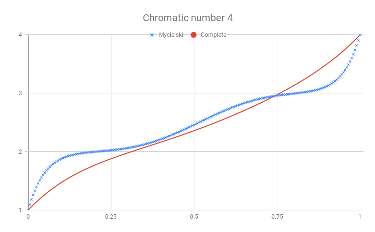
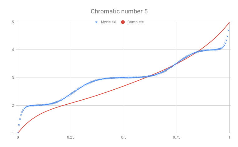
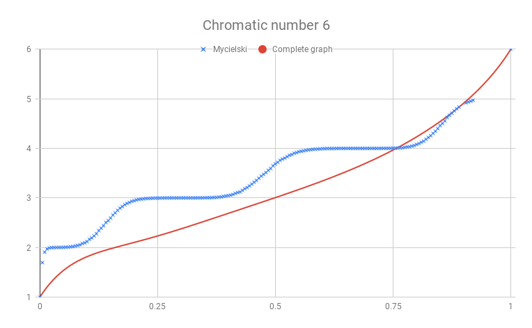
Figure 1: Plots of $\mathbb{E}[\chi(G_{p})]$ for $M_{k}$ (thicker, blue) and $K_{k}$ (thinner, red) for $k=4,5,6$

For every $G$, it is not difficult to see that $\chi(M(G))=\chi(G)+1$. Thus, since $\chi(M_{k})=k$, Conjecture 2 asserts that $\mathbb{E}[\chi((M_{k})_{p})]\geq\mathbb{E}[\chi(G(k,p))]$ whenever $p\leq\frac{1}{2}$, which—from Figure 1—we see to be true for $4\leq k\leq 6$. Although these plots agree with Conjecture 2 for $p\leq\frac{1}{2}$, we also see that each has values of $p$ near $1$ for which the inequality of our conjecture fails (because $M_{k}$ has more edges than the complete graph on $k$ vertices). In fact, we show that this is unavoidable in the following sense.

See 3

Proof.

An edge-critical graph is one in which every proper subgraph has lower chromatic number. For each $n\geq 3$, there are graphs $G$ with arbitrarily many edges and fixed $\chi(G)=n$—for instance we could obtain such a graph by iterating the Mycielskian construction starting with a large odd cycle. Thus, we can select an edge-critical $G$ such that $1-(1-p)|E(H)|>p^{|E(G)|}$ and $\chi(G)=\chi(H)=n$. For this $G$, edge-criticality implies $\mathbb{E}[\chi(G_{p})]\leq np^{|E(G)|}+(n-1)(1-p^{|E(G)|})=n-1+p^{|E(G)|}<n-(1-p)|E(H)|.$ On the other hand, for any graph $\chi(H)-\mathbb{E}[\chi(H_{p})]\leq(1-p)|E(H)|$ since $(1-p)|E(H)|$ is equal to the expected number of edges removed going from $H$ to $H_{p}$, and removing an edge lowers the chromatic number by at most 1. Thus we have $\mathbb{E}[\chi(G_{p})]<n-(1-p)|E(H)|\leq\mathbb{E}[\chi(H_{p})]$, as desired. ∎

As an aside, it is interesting to note the apparent “plateaus” in the graphs of $\mathbb{E}[\chi((M_{k})_{p})]$. For values of $p$ in these plateaus, it seems reasonable to conjecture that the distribution of $\chi((M_{k})_{p})$ is tightly concentrated on an integer value, and it would be interesting to study these graphs for large $k$.

5 Proof of Theorem 4

Conjecture 2 naturally leads to the following definition.

Definition 1.

For a family of graphs $\mathcal{F}$ and fixed $p\in(0,1)$, we say that $G\in\mathcal{F}$ is an $n$-minimizer among $\mathcal{F}$ if $\mathbb{E}[\chi(H_{p})]\geq\mathbb{E}[\chi(G_{p})]$ for all $H\in\mathcal{F}$ with $\chi(H)=\chi(G)=n$.

In the language of $n$-minimizers, Conjecture 2 states that for all $p\leq\frac{1}{2}$, and all $n$, $K_{n}$ is an $n$-minimizer among all graphs. And for $n\geq 3$, Theorem 3 states that no graph is an $n$-minimizer for all $p\in(1-\varepsilon,1]$.

For small chromatic numbers, Conjecture 2 is easy to verify, and the case $n\in\{1,2\}$ there is nothing to show. As the first interesting case, the classification of 3-minimizers is given by the following lemma.

Proposition 1.

For each $p\in(0,\frac{1}{2})$, $K_{3}$ is the unique 3-minimizer; for $p=\frac{1}{2}$, every odd cycle is a 3-minimizer; and for each $p\in(\frac{1}{2},1)$, there are no 3-minimizers.

For this, we first need the following easy lemma.

Lemma 1.

Let $G$ be a graph and $H$ a proper subgraph. Then $\mathbb{E}[\chi(H_{p})]<\mathbb{E}[\chi(G_{p})]$ for all $p\in(0,1)$.

Proof of Lemma 1.

For this, we couple $H_{p}$ and $G_{p}$ by first sampling the edges of $H$ and then sampling the remaining edges of $G$. In this coupling we have $H_{p}\subseteq G_{p}$ implying $\chi(H_{p})\leq\chi(G_{p})$. Moreover, strict inequality is possible (e.g., if $H_{p}$ does not have any edges but $G_{p}$ does). ∎

Proof of Proposition 1.

Since every graph with chromatic number at least $3$ contains an odd cycle, we need only consider odd cycles in determining which graphs are $3$-minimizers. Letting $C^{2k+1}$ denote the odd cycle on $2k+1$ vertices, we have

$$\mathbb{E}[\chi(C^{2k+1}_{p})]=2+p^{2k+1}-(1-p)^{2k+1}.$$

For $0<p<\frac{1}{2}$, this is minimized when $k=3$. When $p=1/2$, this quanity is $2$ independent of $k$. And for $p\in(\frac{1}{2},1)$, this quantity converges to $2$ from above as $k\to\infty$. ∎

In light of this, (and the four-color theorem for planar graphs) to finish the proof of Theorem 4, we need only prove that for $p\leq\frac{1}{2}$, $K_{4}$ is the unique $4$-minimizer among all planar graphs.

Proposition 2.

For all $p\in(0,\frac{1}{2}]$, $K_{4}$ is the unique 4-minimizer among planar graphs.

Proof sketch.

Our proof relies on some rather involved case analysis, which we move to an appendix for ease of reading. Here, we provide a very high-level proof sketch.

Our starting point is the Grünbaum–Aksionov theorem that every planar graph with at most three 3-cycles is 3-colorable [10, 1]. From this, we construct a finite list of graphs that must be contained in any planar graph with chromatic number $4$ somewhat simplifying along the way for our purposes. After this, we simply compare $K_{4}$ to this finite list of subgraphs and note that the expected chromatic number of $K_{4}$ is the greatest. Full details available in the appendix. ∎

6 Discussion of Theorem 1 and a question of [17]

Although the Hoffman bound is often a poor estimate for $\chi(G)$, there are nonetheless natural families of graphs for which our spectral result is the only known general result providing the bound of question 1. For example, we will present the Kneser graphs, whose parameters are chosen so that none of the previously known bounds discussed in the introduction establishes Bukh’s conjecture, yet Theorem 1 does.

The Kneser graph with parameters $n\geq k\geq 0$, denoted $KG_{n,k}$, is the graph whose vertices are indexed by the $k$-element subsets of $\{1,2,\ldots,n\}$ and for which two vertices are adjacent iff the corresponding sets are disjoint. In this language, the classic Erdős–Ko–Rado theorem [8] states for $n\geq 2k$, $\alpha(KG_{n,k})={n-1\choose{k-1}}$, and a celebrated result of Lovász [13] establishes $\chi(KG_{n,k})=n-2k+2$.

It is well-known that the Kneser graphs are regular with $\lambda_{max}=\left(\begin{subarray}{c}n-k\\ k\end{subarray}\right)$ and $\lambda_{min}=-\left(\begin{subarray}{c}n-k-1\\ k-1\end{subarray}\right)$ [9]. Thus, our spectral bound gives almost surely

$$\chi((KG_{n,k})_{p})\geq\frac{\lambda_{\textup{max}}(G)}{-\lambda_{\textup{min}}(G)+(C/p)(\sqrt{\Delta}+\sqrt{\log(|V|)})}=\frac{{{n-k}\choose k}}{{{n-k-1}\choose k-1}+(C/p)\left[\sqrt{{{n-k}\choose k}}+\sqrt{\log{{n}\choose k}}\right]}.$$

For $k\geq 3$ (to avoid trivialities), the denomonitor is dominated by the first term, which gives almost surely

$$\chi((KG_{n,k})_{p})\geq\frac{{{n-k}\choose k}}{(1+\varepsilon_{p}){{n-k-1}\choose k-1}}=\frac{n-k}{(1+\varepsilon_{p})k},$$

for some $0<\varepsilon_{p}$ tending to $0$ as $n\to\infty$.

For $k\ll n$ and $p$ fixed, this gives a lower bound on $\chi((KG_{n,k})_{p})$, which is on the order of $n$, which asymptotically matches the trivial upper bound $\chi(KG_{n,k})$. Thus, this establishes Bukh’s conjecture for Kneser graphs in this regime, and for sufficiently small values of $k$ (e.g., $k\geq 3$ fixed) ours is the only general bound able to do this. Although, for Kneser graphs in particular, $\chi((KG_{n,k})_{p})$ is already well-understood for a wide range of $p$ by completely different methods [12].

Finally, we briefly turn our attention to a question of Shinkar, which we resolve negatively. Hoping to use (1.1) to resolve question 1 for all graphs, Shinkar  [17] asks the following:

Question 2 (Shinkar).

Is it true that every graph $G$ contains an induced subgraph $G^{\prime}\subset G$ such that $\chi(G^{\prime})\geq c\cdot\chi(G)$, and $\alpha(G^{\prime})\leq C\frac{|V(G^{\prime})|}{\chi(G^{\prime})}$ for some absolute constants $C,c>0$?

The answer to this question is ‘no,’ as shown by Kneser graphs. Namely, Sudakov and Verstraëte  [18] observe that if $H$ is any induced subgraph of $KG_{sk,k}$, then $|V(H)|/\alpha(H)\leq s$. This is because given $|V(H)|$ subsets of $\{1,2,\dots,sk\}$ of size $k$, by the pigeonhole principle there exists $i\in\{1,2,\dots,sk\}$ such that $i$ is contained in at least $k|V(H)|/sk$ of the sets of size $k$, and because these sets all intersect, the corresponding vertices form an indpendent set of size at least $|V(H)|/s$. With this, we see that for sufficiently large $k$, the Kneser graphs $KG_{3k,k}$ provide an infinite family of counterexamples to Question 2.

Appendix A Appendix: Proof of Proposition 2

Proof of Proposition 2.

We will start by categorizing a particular family of graphs. Define $\mathbb{F}_{4}$ as a collection of graphs such that each $G\in\mathbb{F}_{4}$ has exactly 4 triangles and satisfies the following two conditions:

Condition 1: For every triangle $T\subset G$ and every vertex $p\in V(T)$, either

1. $p$ is not contained in any other triangle, or

2. $p$ is contained in another triangle, and $T$ intersects some triangle $T^{\prime}$ in an edge containing $p$

The motivation for this condition is that if $G$ fails it, we can “separate” $G$ at $p$ as shown below, preserving the number of triangles, and leading to a graph $G^{\prime}$ whose subgraph has a lower expected chromatic number (For every subgraph $H\subset G$, there is an equivalent subgraph $H^{\prime}\subset G^{\prime}$ obtained by separating $H$ at the same vertices where we split $G$. Clearly, then any coloring of the vertices on $H$ can be copied onto $H^{\prime}$, where separated vertices both share the same color as the original vertex.)

Condition 2: For any graph $G\in\mathbb{F}_{4}$, $G$ has no proper subgraphs $H$ containing four triangles.

As a result, we know that every edge in $G$ is an edge of some triangle of $G$. Now consider the four triangles of $G$, $T_{1}$, $T_{2}$, $T_{3}$, and $T_{4}$. $G$ is uniquely defined by how we identify the edges of each $T_{i}$ to the other triangles (remember, we just identify cannot identify individual points, as this may lead to a problem with our first condition). Informally, we can construct $\mathbb{F}_{4}$ in the following manner: start with $T_{1}$, and let $\mathbb{G}_{2}$ be all the graphs obtained by identifying the edges of $T_{2}$ with the edges of $T_{1}$. Construct $\mathbb{G}_{3}$ by identifying the edges of $T_{3}$ with the edges of each $G\in\mathbb{G}_{2}$. Finally, construct $\mathbb{G}_{4}$ by identifying the edges of $T_{4}$ with the edges of each $G\in\mathbb{G}_{3}$. There will certainly be graphs in $\mathbb{G}_{4}$ that do not have exactly four triangles; however, we can be sure that $\mathbb{F}_{4}\subset\mathbb{G}_{4}$.

Some brief observations that will make our constructions of the $\mathbb{G}_{i}$ easier:

• For any given triangles $T_{i}$ and $T_{j}$, we can only identify at most one of the edges from each triangle. If $T_{i}$ and $T_{j}$ share two edges, they must share all three edges, and would therefore be the same triangle. We can ignore these cases, as we wish for the four $T_{k}$ to represent four distinct triangles in the identification graphs.

• The process of identifying the edges of the $T_{i}$ in turn is commutative. Therefore, if our final graph has $n$ components, we can choose the order of identification such that if the edges of $T_{j}$ are not identified to any $T_{i}$ for $i<j$, then the edges of all $T_{k}$, $k>j$ will also not be identified to any $T_{i}$. In other words, we can always choose to have $T_{j}$’s edges only be identified to the edges of exactly one component of $H\in\mathbb{G}_{j-1}$

Now, we can start constructing $\mathbb{G}_{1}$, $\mathbb{G}_{2}$, $\mathbb{G}_{3}$ and $\mathbb{G}_{4}$. The first two are trivial.

$\mathbb{G}_{1}$

$\mathbb{G}_{2}$

$\mathbb{G}_{3}$

Consider $B_{1}$. We can construct exactly two distinct (up to isomorphism) child graphs, by either identifying none of the edges of $T_{3}$, or identifying one of the edges of $T_{3}$ to one of the component triangles. We cannot do anything more, as this would result in identifying two edges to the same triangle or connecting to separate components:

Now consider the second graph of $\mathbb{G}_{2}$, $B_{2}$. If we do not identify $T_{3}$ to any edge, then we get a graph isomorphic to $H_{2}$. If we identify one edge of $T_{3}$ to any of the four external edges, we will obtain the same graph (up to isomorphism):

If we identify one edge of $T_{3}$ to the center edge of $B_{1}$, then we obtain the following graph:

Finally, suppose we identify two edges of $T_{3}$ to two edges of $B_{2}$. We cannot identify them to two edges from the same triangle in $B_{2}$. Therefore, we can identify neither of the two edges to the center edge of $B_{2}$, as any other edge would lie on the same triangle as the center edge. Therefore, we have two options: identify two edge, one from each triangle, that are adjacent, or non adjacent. First, a larger visual:

Without loss of generality, assume that the two edges we are identifying from $T_{3}$ are {1,2} and {2,3}. Assume we identify these two edges with the edges {A,B} and {B,D}. We must do this identification by identifying 2 to B, and we are left with the following graph:

(Note, the graph $C_{5}$ has four triangles. However, one of these triangles is not identified to any of $T_{1}$, $T_{2}$, or $T_{3}$, but is composed of one edge from each.)

Now suppose that we identify the same two edges of $T_{3}$ to the edges {A,B} and {C,D}. In whatever manner we choose to identify the individual vertices, we will have to identify either vertex C or D with vertex A or B. This would necessarily result in the destruction of one of the previous triangles in $B_{2}$. Therefore, we cannot identify any two edges from $T_{3}$ to non-adjacent edges on $B_{2}$.

Therefore, we have completely categorized $\mathbb{G}_{3}$.

$\mathbb{G}_{4}$

In the same manner as before, we can generate the first two graphs of $\mathbb{G}_{4}$ from $C_{1}$:

Consider $C_{2}$. If $T_{4}$ is disjoint, then we obtain the same graph as $D_{2}$. By the same reasoning as before, if we identify one edge of $T_{4}$ to an edge of the triangular component of $C_{2}$, one edge to an external edge of the larger component of $C_{2}$, one edge to the internal edge of the larger component of $C_{2}$, or two edges (in the only way possible) to the larger component of $C_{2}$, we obtain, respectively:

Consider $C_{3}$. If we add a disjoint triangle, we will obtain $D_{4}$ again. If we identify one edge of $T_{4}$ to the exterior edge of $C_{3}$ lying in the center triangle, to one of other exterior edges, or to an interior edge of $C_{3}$, we will obtain, respectively:

Suppose we identify two edges of $T_{4}$ to $C_{3}$:

Without loss of generality let the two edges of $T_{4}$ be {1,2} and {2,3}. Our two edges on $C_{3}$ either i) lie on a subgraph isomorphic to $B_{2}$ or ii) one edge is {A,B} or {A,C}, and the other is {B,E} or {D,E}. In case i), WLOG let the subgraph of $C_{3}$ be the induced subgraph on vertices C, B, D, and E. We know from our earlier argument that we must either identify {1,2} and {2,3} to {C,B} and {B,E}, or {C,D} and {D,E}. With either choice, we obtain the graph:

In case ii), if we identify {1,2} to {E,B} and {2,3} to {B,A}, we obtain the following graph:

If we identify {1,2} to {A,B} and {2,3} to {D,E} (equivalent to identifying {1,2} to {A,C} and {2,3} to {B,E}), then we must identify vertex 2 to A and E (otherwise, we will collapse two triangles). At this point, the graph we will obtain will contain a copy of $K_{4}$, so we need not consider it for $\mathbb{F}_{4}$.

If we identify {1,2} to {A,C} and {2,3} to {D,E}, then we must identify vertex 2 to A and E again. By the same logic as before, we can ignore this graph.

Consider the graph $C_{4}$. If $T_{4}$ is disjoint, then we obtain $D_{5}$. If we identify one edge of $T_{4}$ to one of the exterior six edges, we obtain $D_{9}$. If we identify the edge of $T_{4}$ to the central edge shared by the other three triangles, we obtain the graph:

If we identify two edges of $T_{4}$, then we must identify them to edges lying in a subgraph of $C_{4}$ isomorphic to $B_{2}$. Therefore, the graph we obtain must have a copy of $K_{4}$.

Finally, consider $C_{5}$. Identifying edges in $T_{4}$ to edge in $C_{5}$ in such a way such that we preserve the uniqueness of all the triangles will force us to have a copy of $K_{4}$ in our resulting graph. Therefore, we can ignore these graphs. For formality’s sake, we should identify $T_{4}$ with the triangle in $C_{5}$ comprised of one edge from each of the previous three $T_{i}$. We then obtain the graph $D_{13}$ (which is the same graph as $C_{5}$):

Now that we have categorized $\mathbb{G}_{4}$, we can pull $\mathbb{F}_{4}$ as a subset from these graphs. We see that $D_{6}$ and $D_{10}$ contain copies of $D_{13}$ ($K_{4}$). However, every other graph satisfies the properties for $\mathbb{F}_{4}$. Therefore, the graphs of $\mathbb{F}_{4}$ are as follows:

Using Grünbaum’s result, we note that every 4-colorable planar graph must have at least four 3-cycles. By the restrictions we placed on the graphs of $\mathbb{F}_{4}$, we know that for any 4-colorable planar graph $G$, there must be an $G^{\prime}\subset G$ and $H\in\mathbb{F}_{4}$ such that either $G^{\prime}\cong H$, or $G^{\prime}$ is an edge-minimal subgraph of $G$ with four triangles such that $\mathbb{E}[\chi(G^{\prime}_{p})]\geq\mathbb{E}[\chi H_{p})]$ for all $p$ (this would be the case where we can separate at least one vertex in $G^{\prime}$). Therefore, we must only consider the graphs in $\mathbb{F}_{4}$ along with the expected chromatic numbers of their random subgraphs to determine whether $K_{4}$ is a 4-minimizer. Note that in the following, we have renamed the graphs of $\mathbb{F}_{4}$ for convenience:

From the expected values of the different configurations, we see that if $G$ is a planar 4-minimizer, then either it must be $K_{4}$, or it must be a 4-critical supergraph of $G^{8}$. Let us consider the graph of $G^{8}$ a little more carefully (this time drawn in a planar fashion):

No matter how we draw $G^{8}$, we will always have a subgraph structure of a 3-cycle enclosing a fourth point that connects to two of the points of the 3-cycle. Without loss of generality then, let us suppose that the 3-cycle $C_{3}$ is composed of points $A$, $B$, and $C$, with interior point $D$:

Now treat $G^{8}$ as the subgraph of a larger graph $H$. Consider Int($C_{3}$) (the subgraph induced by the vertices on and inside $C_{3}$) and Ext($C_{3}$) (the subgraph induced by the vertices on and outside $C_{3}$). Because the coloring of $C_{3}$ is independent of the structure of $H$ (up to translation), the coloring of Int($C_{3}$) is independent of the coloring of Ext($C_{3}$). Therefore, if $H$ is 4-colorable, then at least one of Int($C_{3}$) or Ext($C_{3}$) must be 4-colorable. However, because Int($C_{3}$)$\setminus C_{3}$ and Ext($C_{3}$)$\setminus C_{3}$ are both nonempty, $H$ cannot be critically chromatic. Therefore, there exists no planar 4-critical chromatic graph containing $G^{8}$. Therefore, $K_{4}$ is the unique planar 4-minimizer for $p=\frac{1}{2}$.

In general, the proof that $K_{4}$ is the unique planar 4-minimizer for all $p\in(0,\frac{1}{2}]$ follows from the same reasoning. Namely, we simply find polynomial expressions in $p$ for the expected values of each our different triangle configurations that must appear—each such polynomial is relatively easy to calculate, but they are emphatically awful to look at. Among these, the polynomial for $K_{4}$ is the least for all $p\in(0,1/2]$, which follows from routine computations. ∎

References

- [1] V. Aksionov, On continuation of 3-colouring of planar graphs. diskret. anal. novosibirsk 26 (1974), 3–19.
- [2] N. Alon, M. Krivelevich, and B. Sudakov, Subgraphs with a large cochromatic number, Journal of Graph Theory, 25 (1997), pp. 295–297.
- [3] A. Bandeira and R. v. Handel, Sharp nonasymptotic bounds on the norm of random matrices with independent entries, The Annals of Probability, 44 (2016), p. 2479–2506.
- [4] H. Bennett, D. Reichman, and I. Shinkar, On percolation and NP-hardness, no. 55, 2016.
- [5] B. Bollobás, The chromatic number of random graphs, Combinatorica, 8 (1988), pp. 49–55.
- [6] B. Bukh, Interesting problems that I cannot solve. Problem 2. URL: http://www.borisbukh.org/problems.html.
- [7] P. Devlin and J. Kahn, On “stability” in the Erdős–Ko–Rado theorem, SIAM Journal on Discrete Mathematics, 30 (2016), pp. 1283–1289.
- [8] P. Erdős, C. Ko, and R. Rado, Intersection theorems for systems of finite sets, Quarterly Journal of Mathematics, Oxford Series, 2 (1961), pp. 313–320.
- [9] C. Godsil and G. Royle, Algebraic Graph Theory, Springer, New York, 2001.
- [10] B. Grünbaum, Grötzsch’s theorem on -colorings., The Michigan Mathematical Journal, 10 (1963), pp. 303–310.
- [11] A. J. Hoffman and L. Howes, On eigenvalues and colorings of graphs, ii, Annals of the New York Academy of Sciences, 175 (1970), pp. 238–242.
- [12] A. Kupavskii, On random subgraphs of Kneser and Schrijver graphs, Journal of Combinatorial Theory, Series A, 141 (2016), pp. 8–15.
- [13] L. Lovász, Kneser’s conjecture, chromatic number, and homotopy, Journal of Combinatorial Theory, Series A, 25 (1978), pp. 319–324.
- [14] B. Mohar and H. Wu, Fractional chromatic number of a random subgraph, (2018). URL: https://arxiv.org/pdf/1807.06285.pdf.
- [15] J. Mycielski, Sur le coloriage des graphes, in Colloq. Math, vol. 3, 1955, p. 9.
- [16] O. Ore, Theory of graphs, vol. 38, American Mathematical Society, 1962.
- [17] I. Shinkar, On coloring random subgraphs of a fixed graph. URL: https://arxiv.org/pdf/1612.04319.pdf., 2016.
- [18] B. Sudakov and J. Verstraëte, Cycles in graphs with large independence ratio, Journal of Combinatorics, 2 (2011), pp. 83–102.