Line-driven disc wind in near-Eddington active galactic nuclei: decrease of mass accretion rate due to powerful outflow

Abstract

Based on recent X-ray observations, ultra-fast outflows from supermassive black holes are expected to have enough energy to dramatically affect their host galaxy but their launch and acceleration mechanisms are not well understood. We perform two-dimensional radiation hydrodynamics simulations of UV line-driven disc winds in order to calculate the mass loss rates and kinetic power in these models. We develop a new iterative technique which reduces the mass accretion rate through the inner disc in response to the wind mass loss. This makes the inner disc is less UV bright, reducing the wind power compared to previous simulations which assumed a constant accretion rate with radius. The line-driven winds in our simulations are still extremely powerful, with around half the supplied mass accretion rate being ejected in the wind for black holes with mass $10^{8}$–$10^{10}\,M_{\odot}$ accreting at $L/L_{\rm Edd}=0.5$–$0.9$. Our results open up the way for estimating the growth rate of supermassive black hole and evaluating the kinetic energy ejected into the inter stellar medium (active galactic nuclei feedback) based on a physical model of line-driven disc winds.

1 Introduction

Supermassive black holes (SMBHs) are found in the centre of almost all known galaxies, and their masses are observed to correlate with the mass of stars in their host galaxy bulge. This implies that the star formation powered growth of the galaxy is linked to the accretion powered growth of its black hole via feedback (e.g., Magorrian et al., 1998; Ferrarese & Merritt, 2000; Gebhardt et al., 2000; Tremaine et al., 2002). The details of this feedback mechanism are not well understood, but winds powered by the accretion flow onto the black hole are likely to play a role. This is supported by recent observations of ultra-fast outflows (UFOs) in active galactic nuclei (AGNs). These winds are identified via blueshifted absorption lines of highly ionized iron (FeXXV and/or FeXXVI) detected in the X-ray band. These were first detected in a few bright quasars (e.g., Chartas et al., 2002; Pounds et al., 2003; Reeves et al., 2003), but more recent systematic studies of archival data show that these are likely a common feature in AGN (Tombesi et al., 2010, 2011, 2012a; Gofford et al., 2013, 2015). The typical outflow velocity is $0.1$–$0.3c$, where $c$ is the speed of light, giving an estimate for the kinetic power of (0.1–10%)$L_{\rm Edd}$, where $L_{\rm Edd}$ is the Eddington luminosity (Tombesi et al., 2012a; Gofford et al., 2015). This is large enough to affect the properties of the host galaxy, possibly setting the $M$–$\sigma$ relation (King, 2003).

The terminal velocity of a wind typically is of order the escape velocity from its launch point, so the fast velocity of the UFOs means that they should be launched from the accretion disc close to the SMBH. There are only a few potential mechanisms to drive a wind from such high gravity regions: radiation pressure on electrons for super-Eddington sources (super-Eddington winds), radiation pressure on UV line transitions (UV line-driven winds), and magnetic fields (magnetic winds). Most UFOs are seen in sources which are not above the Eddington limit, leaving only UV line driving or magnetic winds. UV line driving requires that the material has low ionization state, where radiation pressure on the multiple UV spectral lines produces a force, pushing material away from the SMBH. Theoretical studies of UV line-driven winds started from an analytic approach (Murray et al., 1995) but now include both hydrodynamic simulations (Proga et al., 2000; Proga & Kallman, 2004, hereafter PK04) and non-hydrodynamic calculations of streamlines from ballistic trajectories (Risaliti & Elvis, 2010; Nomura et al., 2013). The line force is $10$–$1000$ times larger than that due to radiation on electrons when the material is in a low-ionization state (Stevens & Kallman, 1990), leading to a high-velocity disc wind. However, the observed very high ionization state of the UFOs is apparently in conflict with UV line driving (Tombesi et al., 2010), but this mechanism can still work if the wind is only highly ionized after it has reached terminal velocity (e.g., Hagino et al. 2015; Mizumoto et al. 2020 in preparation)

Simulations of UV line-driven winds show that UV line driving can indeed produce powerful winds from sub-Eddington AGN despite X-ray irradiation (Proga et al. 2000; PK04; Risaliti & Elvis 2010; Nomura et al. 2013). These simulations include the effect of a central X-ray source in ionizing the wind, and typically show that a UV line-driven wind is launched from the UV bright disc, lifting material up to where it intercepts more of the hard X-ray coronal radiation, so is overionized. This removes the UV transitions, so the line force drops and the outflow stalls and falls back, producing a vertical structure which shields material further out from the ionizing radiation. The failed wind region becomes larger and larger until the shielding is sufficient for material in the outer regions to reach its escape velocity before it is overionized by the X-ray flux.

These hydrodynamic models predict the density, ionization state and velocity of material around the disc. However, the absorption features in the outflow are due to multiple line and bound-free transitions, so a full prediction of the spectral features for detailed comparison to observations requires postprocessing of the results using a full photo-ionization radiation transfer code. This is a very intensive calculation so has only been performed for a single hydrodynamics simulation, that of PK04 for a black hole mass of $M_{\rm BH}=10^{8}\,M_{\odot}$ and luminosity of $L/L_{\rm Edd}=0.5$ for a central X-ray source with $L_{\rm X}=0.1L_{\rm D}$, where $L_{\rm D}$ is the luminosity of the accretion disc. This set of parameters resulted in a funnel-shaped wind with high ionization and high velocity of $\sim 0.05$–$0.1c$, carrying away around half of the total mass accretion rate though the disc. This can produce blueshifted absorption lines qualitatively similar to those seen in the UFOs (Schurch et al., 2009; Sim et al., 2010; Higginbottom et al., 2014), though this particular simulation does not produce high enough wind velocity to fit the fastest UFOs observed (e.g., PDS456, Reeves et al., 2009). Instead, magnetic winds can easily explain the high-velocity, high ionization outflowing matter (e.g, Blandford & Payne, 1982; Konigl & Kartje, 1994; Fukumura et al., 2015), but this model requires that the magnetic field lines form a specific global topology (Blandford & Payne, 1982) which cannot (currently) be determined ab initio.

Instead, our previous works Nomura et al. (2016) and Nomura & Ohsuga (2017, hereafter N17) calculated radiation hydrodynamics simulations of UV line-driven winds over a much wider parameter space of black hole mass, mass accretion rate, and X-ray irradiation. These can be used to estimate the absorption column along each line of sight, velocity and typical ionization state of the material for a rough comparison with the data. The results of N17 show that these UV line-driven wind hydrodynamics simulations do indeed span the range observed in UFOs, and also can match the luminosity dependence of the mass outflow rate suggested by Gofford et al. (2015). These results clearly show that UV line-driven winds are energetically consistent with the observed UFOs.

However, all such simulations to date are not self-consistent as they assume a constant accretion rate with radius. Yet many of the predicted winds, especially those at $L/L_{\rm Edd}\gtrsim 0.5$, have mass loss rate, $\dot{M}_{\rm out}$, which is a large fraction of the mass accretion rate through the disc. This is important as the most powerful UFOs observed are in sources with similarly large $L/L_{\rm Edd}$, where the winds should expel large amounts of mass from the accretion disc.

In this paper, we improve the calculation method of the radiative hydrodynamic code of N17 so as to consider the reduction of mass accretion rate due to the loss of mass and angular momentum in the UV line-driven disc wind. This reduces the UV flux from the inner disc, but powerful UV winds are still produced, and carry enough energy and momentum to impact on the host galaxy growth.

2 Method

2.1 Basic equations

We modify the calculation method of N17 so as to satisfy the conservation law of the total mass of the disc and winds. We briefly review our calculation method, and then describe how we incorporate the reduction in mass accretion rate through the inner disc caused by the wind losses.

The simulations use spherical polar coordinate $(r,\theta,\varphi)$, where $r$ is the distance from the origin of the coordinate, $\theta$ is the polar angle, and $\varphi$ is the azimuthal angle. We perform the calculation in two-dimensions as we assume the axial symmetry about the rotation axis of the disc. The basic equations of the hydrodynamics are the equation of continuity,

$$\frac{\partial\rho}{\partial t}+\nabla\cdot(\rho\mbox{\boldmath$v$})=0,$$ (1)

the equations of motion,

$$\frac{\partial(\rho v_{r})}{\partial t}+\nabla\cdot(\rho v_{r}\mbox{\boldmath$v$})=-\frac{\partial p}{\partial r}+\rho\Bigg{[}\frac{v_{\theta}^{2}}{r}+\frac{v_{\varphi}^{2}}{r}+g_{r}+f_{{\rm rad},\,r}\Bigg{]},$$ (2)

$$\frac{\partial(\rho v_{\theta})}{\partial t}+\nabla\cdot(\rho v_{\theta}\mbox{\boldmath$v$})=-\frac{1}{r}\frac{\partial p}{\partial\theta}+\rho\Bigg{[}-\frac{v_{r}v_{\theta}}{r}+\frac{v_{\varphi}^{2}}{r}\cot\theta+g_{\theta}+f_{{\rm rad},\,\theta}\Bigg{]},$$ (3)

$$\frac{\partial(\rho v_{\varphi})}{\partial t}+\nabla\cdot(\rho v_{\varphi}\mbox{\boldmath$v$})=-\rho\Bigg{[}\frac{v_{\varphi}v_{r}}{r}+\frac{v_{\varphi}v_{\theta}}{r}\cot\theta\Bigg{]},$$ (4)

and the energy equation,

$$\frac{\partial}{\partial t}\Bigg{[}\rho\Bigg{(}\frac{1}{2}v^{2}+e\Bigg{)}\Bigg{]}+\nabla\cdot\Bigg{[}\rho\mbox{\boldmath$v$}\Bigg{(}\frac{1}{2}v^{2}+e+\frac{p}{\rho}\Bigg{)}\Bigg{]}=\rho\mbox{\boldmath$v$}\cdot\mbox{\boldmath$g$}+\rho\mathcal{L},$$ (5)

where $\rho$ is the mass density, $v$$=(v_{r},\,v_{\theta},\,v_{\varphi})$ are the velocities, $p$ is the gas pressure, $e$ is the internal energy per unit mass, $g$$=(g_{r},\,g_{\theta})$ is the gravitational acceleration of the black hole located at $(r,\theta)=(z_{0},\pi)$, and $f$${}_{\rm rad}=(f_{{\rm rad},r},\,f_{{\rm rad},\theta})$ is the radiation force per unit mass (see Section 2.2 for detail). An adiabatic equation of state $p/\rho=(\gamma-1)e$ with $\gamma=5/3$ is assumed in our calculations.

In the last term of Eq. 5, $\mathcal{L}$ is the approximate formula of the net heating rate introduced by Blondin (1994),

$$\mathcal{L}=n^{2}(G_{\rm Compton}+G_{\rm X}-L_{\rm b,l}),$$ (6)

where, $n$ is the number density, $G_{\rm{Compton}}$ is the heating rate via the Compton scattering,

$$G_{\rm{Compton}}=8.9\times 10^{-36}\xi(T_{\rm X}-4T)\,{\rm erg\,cm^{-3}\,s^{-1}},$$ (7)

$G_{\rm X}$ is the difference between the heating rate by the X-ray photoionization and the cooling rate via the recombination,

$$G_{\rm X}=1.5\times 10^{-21}\xi^{1/4}T^{-1/2}(1-T/T_{\rm X})\,{\rm erg\,cm^{-3}\,s^{-1}},$$ (8)

and $L_{\rm{b,l}}$ is the cooling rate by the bremsstrahlung and line emission,

$$L_{\rm{b,l}}=3.3\times 10^{-27}T^{1/2}+1.7\times 10^{-18}\xi^{-1}T^{-1/2}$$

$$\times\exp(-1.3\times 10^{5}/T)+10^{-24}\,{\rm erg\,cm^{-3}\,s^{-1}}.$$ (9)

In Eq.9, the first term represents the effect of the bremsstrahlung and the last two terms show the line coolong in an optically thin atmosphere. The temperature $T$ is obtained by $T=\mu m_{\rm p}p/k_{\rm B}\rho$, where $\mu$ (=0.5) is the mean molecular weight, $m_{\rm p}$ is the proton mass, and $k_{\rm B}$ is the Boltzmann constant. The ionization parameter, $\xi$, is defined as

$$\xi=\frac{4\pi F_{\rm X}}{n}\,{\rm erg\,s^{-1}\,cm},$$ (10)

where $F_{\rm X}$ is the X-ray flux. In the present study, the X-ray is assumed to come from the point source at the centre with luminosity $L_{\rm X}=f_{\rm X}L_{\rm D}$, where $f_{\rm X}$ is a parameter. We also assume the temperature of the X-ray radiation to be $T_{\rm X}=10^{8}\,\rm{K}$. The X-ray flux is attenuated via the absorption of which the cross section is set to be $\sigma_{\rm X}=\sigma_{\rm e}$ for $\xi>10^{5}$, or $100\sigma_{\rm e}$ for $\xi\leq 10^{5}$, where $\sigma_{\rm e}$ is the mass-scattering coefficient for free electrons. Such a treatment is employed in previous works (Proga et al., 2000; Nomura et al., 2016, N17). We note that the scattered and reprocessed photons are ignored in our simulations (see also Section 4.2).

2.2 Line force

The radiation force in Eq.2 and Eq.3 is described as

$${\mbox{\boldmath$f$}_{\rm rad}}=\frac{\sigma_{\rm e}\mbox{\boldmath$F$}_{\rm D}}{c}+\frac{\sigma_{\rm e}\mbox{\boldmath$F$}_{\rm line}}{c}M,$$ (11)

where $F$_D is the radiation flux of the disc emission integrated by the wavelength throughout the entire range, and $F$_line is the line-driving flux (UV flux), which is the same as $F$_D but integrated across the UV transition band of $200$–$3200\,$Å. Both fluxes are calculated by integrating the radiation from the inner hot region of the disc, where the effective temperature is larger than $3\times 10^{3}\,{\rm K}$. We divide the disc surface into $4096$ grids for radial direction and $4096$ grids for azimuthal direction, and numerically calculate $\mbox{\boldmath$F$}_{\rm D}$ and $\mbox{\boldmath$F$}_{\rm line}$. The radial components of these fluxes are attenuated due to electron scattering, of which the optical depth is measured from the origin of the coordinate. On the other hand, $\theta$-components of $\mbox{\boldmath$F$}_{\rm D}$ and $\mbox{\boldmath$F$}_{\rm line}$ are supposed not to be diluted.

The force multiplier, $M$, is defined by Stevens & Kallman (1990),

$$M(t,\xi)=kt^{-0.6}\Biggl{[}\frac{(1+t\eta_{\rm{max}})^{0.4}-1}{(t\eta_{\rm{max}})^{0.4}}\Biggr{]}.$$ (12)

Here, $t$ is the local optical depth parameter written as,

$$t=\sigma_{\rm e}\rho v_{\rm{th}}\Bigl{|}\frac{dv}{ds}\Bigr{|}^{-1}.$$ (13)

Here, the thermal speed, $v_{\rm th}$, is set to $20\,{\rm km\,s^{-1}}$ that corresponds to the thermal speed of the hydrogen gas of the temperature of $25,000\,{\rm K}$. The velocity gradient, $dv/ds$, depends on the direction of each light-ray from the disc surface to the point of interest. However, in order to reduce the computational cost, we evaluate $dv/ds$ along the direction of the disc line-driving flux $($$F$${}_{\rm line}/|$$F$${}_{\rm line}|)$ in the same manner as N17. This is because the radiation along this direction is thought to mainly contribute the line force. We note that this assumption gives the line force comparable to that evaluated by employing more accurate method (see Appendix A.1).

In Eq.12, $k$ and $\eta_{\rm{max}}$ are the functions of the ionization parameter $\xi$ as,

$$k=0.03+0.385\exp(-1.4\xi^{0.6}),$$ (14)

and

$$\log_{10}\eta_{\rm{max}}=\left\{\begin{array}[]{ll}6.9\exp(0.16\xi^{0.4})&\log\xi\leq 0.5\\ 9.1\exp(-7.96\times 10^{-3}\xi)&\log\xi>0.5\\ \end{array}\right..$$ (15)

2.3 Iterative method

The main difference in computational method is the treatment of the mass accretion rate. In N17, we assumed the mass accretion rate was constant with radius, as in the standard disc assumptions (Shakura & Sunyaev, 1973). This is valid when the mass outflow rate via the disc wind is relatively small in comparison with the mass accretion rate. However, such a treatment breaks down for the most powerful winds.

Here we extend the code to take into account the reduction in mass accretion rate through the disc caused by the mass outflow rate. We approximate the total mass loss rate $\dot{M}_{\rm out}$ as coming from a single radius, $R_{\rm launch}$. Thus the mass accretion rate for $R\geq R_{\rm launch}$ is the original mass accretion rate supplied through the outer disc, $\dot{M}_{\rm sup}$, but it drops to $\dot{M}_{\rm BH}=\dot{M}_{\rm sup}-\dot{M}_{\rm out}$ for $R<R_{\rm launch}$.

We estimate $R_{\rm launch}$ by conserving angular momentum per unit mass as well as mass. The material lost in the wind retains the angular momentum produced by the Keplerian velocity at the disc surface. Thus $R_{\rm launch}=l^{2}/GM_{\rm BH}$, where $l=\dot{l}_{\rm out}/\dot{M}_{\rm out}$ is the specific angular momentum of the wind material, calculated via integrating over all angles

$$\dot{l}_{\rm out}=4\pi r^{2}\int^{89^{\circ}}_{0}\rho rv_{\varphi}\sin^{2}\theta d\theta,$$ (16)

and

$$\dot{M}_{\rm out}=4\pi r^{2}\int^{89^{\circ}}_{0}\rho v_{r}\sin\theta d\theta,$$ (17)

at the outer boundary.

Our iterative method consists of following procedures.

1. Based on the standard disc model, of which the mass accretion rate is $\dot{M}_{\rm BH}(=\dot{M}_{\rm sup}-\dot{M}_{\rm out})$ for the region of $r<R_{\rm launch}$ and $\dot{M}_{\rm sup}$ for the region of $r\geq R_{\rm launch}$, we calculate the radiation fluxes, $F_{\rm D}$ and $F_{\rm line}$, and set the temperature and the density on the $\theta=\pi/2$ plane (see Section 2.4 for detail). Here note that, for the first iteration step, $\dot{M}_{\rm BH}$ and $R_{\rm launch}$ can be set arbitrary within the range of $0<\dot{M}_{\rm BH}\leq\dot{M}_{\rm sup}$ and $r_{\rm i}\leq R_{\rm launch}<r_{\rm o}$, here $r_{\rm i}$ and $r_{\rm o}$ are the radii at the inner and outer boundaries of the computational box.

2. We perform the hydrodynamics simulations with using above setup and estimate the time averaged mass outflow rate, $\langle\dot{M}_{\rm out}\rangle$, every $2\times 10^{4}R_{\rm S}/c$, where $R_{\rm S}$ is the Schwarzschild radius. We continue the hydrodynamics simulations until the time averaged mass outflow rate is converged within 10%.

3. We update the mass outflow rate with using the convergence value of the time averaged mass outflow rate, $\dot{M}_{\rm out}=\langle\dot{M}_{\rm out}\rangle$. We also update $R_{\rm launch}$ using the updated $\dot{M}_{\rm out}$.

4. If either updated $\dot{M}_{\rm out}$ or $R_{\rm launch}$ deviates from the value of the previous iteration step more than 10%, we return back to the procedure (i). We iterate procedures (i–iii) until $\dot{M}_{\rm out}$ and $R_{\rm launch}$ are converged within 10%.

The number of the iterations to obtain the quasi-steady state by above procedures depends on the parameters ($M_{\rm BH}$ and $\dot{m}_{\rm sup}=\dot{M}_{\rm sup}/\dot{M}_{\rm Edd}$) and initial choice of $\dot{M}_{\rm BH}$ and $R_{\rm launch}$. Here, $\dot{M}_{\rm Edd}$ is defined as $\dot{M}_{\rm Edd}=L_{\rm Edd}/\eta c^{2}$ with the energy conversion efficiency $\eta=0.06$. For example, we need 12 times of iterations for $M_{\rm BH}=10^{8}\,M_{\odot}$ and $\dot{m}_{\rm sup}=0.5$ when we initially employ $\dot{M}_{\rm BH}$=$\dot{M}_{\rm sup}$ (then, we do not need to set $R_{\rm launch}$ because of $\dot{M}_{\rm out}=0$).

As we have mentioned above, in our method, we simply assume that the mass accretion rate discontinuously changes at the radius of $r=R_{\rm launch}$. However, the mass accretion rate would gradually decrease in the wind launching region practically. Also, we assume that the disc is stable and steady. The density and the temperature at the $\theta=\pi/2$ plane are calculated by assuming that the disc is in the hydrostatic equilibrium in the vertical direction. However, Shields et al. (1986) calculated the time dependent disc structure and found that the disc can exhibit the periodic variation of the accretion rate when the mass loss rate is sufficiently large. It is necessary to investigate the time variation of the disc structure via the launching the line-driven winds in order to establish a more realistic wind model. Such a study is left as an important future work.

2.4 Boundary and initial conditions

The hydrodynamics are calculated over a computational domain of $r_{\rm i}=30R_{\rm S}\leq r\leq r_{\rm o}=1500R_{\rm S}$ and $0\leq\theta\leq\pi/2$. The coordinate system is set so that the black hole is located at $r=z_{0}$ and $\theta=\pi$, i.e., at cylindrical radius of 0, but a distance $z_{0}$ below the origin of the coordinate, where $z_{0}=3.1\dot{m}_{\rm sup}R_{\rm S}$ which is the thickness of a standard Shakura-Sunyaev disc at $r_{\rm i}=30R_{\rm S}$ for given $\dot{m}_{\rm sup}$. We divide the computational domain into 100 grids for the radial range and 160 grids for the angular range. We employ the fixed grid size ratios of $\Delta r_{i+1}/\Delta r_{i}=1.05$ and $\Delta\theta_{k}/\Delta\theta_{k+1}=1.066$ in order to resolve the wind launching region. The number of grids is 134 for $z\lesssim 30R_{\rm S}$ and $R\sim 100R_{\rm S}$ where the wind is vertically accelerated and the physical quantities drastically change (left side of the red dashed-dotted line in Fig 4). The wind structure and the mass loss rate do not change so much even if the spatial resolution near the launching region is lowered by employing $\Delta\theta_{k}/\Delta\theta_{k+1}=1.05$, when the grid spacing in the $\theta$-direction becomes several times larger near the $\theta=\pi/2$ plane. In addition, we note that the radiation force starts to accelerate the wind at the point slightly away from the numerical boundary of $\theta=\pi/2$ (see Fig. 4b). This means that the numerical resolution of our present simulations is enough to resolve the launching of the wind.

Boundary and initial conditions are set by the same manner as N17. We employ the axially symmetric boundary at the rotational axis of the accretion disc ($\theta=0$). The outflow boundary conditions are applied at the inner and outer boundaries (at $r_{\rm i}=30R_{\rm S}$ and $r_{\rm o}=1500R_{\rm S}$), where the matter can go out but is not allowed to go into the computational domain. At the boundary of $\theta=\pi/2$, We apply the reflecting boundary condition. At this plane, the radial velocity and the rotational velocity are fixed to be null and the Keplerian velocity. Also the temperature is fixed at the effective temperature of the standard disc model. The density at $\theta=\pi/2$ plane is kept constant at $\rho=\rho_{0}(M_{\rm BH},\varepsilon,r)$ that is the density at the surface of the standard disc,

$$\begin{array}[]{ll}&\rho_{0}(M_{\rm BH},\varepsilon,r)=\bar{\rho}(M_{\rm BH},\varepsilon,r)/(e-1)\\ &=\left\{\begin{array}[]{l}5.24\times 10^{-4}(M_{\rm BH}/M_{\odot})^{-1}(\varepsilon/\eta)^{-2}(r/R_{\rm S})^{3/2}\,{\rm g\,cm^{-3}}\\ \qquad\qquad\qquad\qquad r\leq 18(M_{\rm BH}/M_{\odot})^{2/21}(\varepsilon/\eta)^{16/21}R_{\rm S}\\ 4.66(M_{\rm BH}/M_{\odot})^{-7/10}(\varepsilon/\eta)^{2/5}(r/R_{\rm S})^{-33/20}\,{\rm g\,cm^{-3}}\\ \qquad\qquad\qquad\qquad r>18(M_{\rm BH}/M_{\odot})^{2/21}(\varepsilon/\eta)^{16/21}R_{\rm S}\\ \end{array}\right.\end{array},$$ (18)

where ${\bar{\rho}}(M_{\rm BH},\varepsilon,r)$ is the vertically averaged density of the standard disc model (Shakura & Sunyaev, 1973). We set $\varepsilon=\dot{m}_{\rm sup}$ at the region of $r\geq R_{\rm launch}$ and $\varepsilon=\dot{m}_{\rm BH}=\dot{M}_{\rm BH}/\dot{M}_{\rm Edd}$ at $r<R_{\rm launch}$.

Here we note that the wind structure is insensitive to the density profile at the boundary of $\theta=\pi/2$. This is because that the density at the boundary is too large for the line force to accelerate the matter and the wind is accelerated from the point slightly above the $\theta=\pi/2$ plane, where the density is lower than $\rho_{0}(M_{\rm BH},\varepsilon,r)$ (see also Appendix 2 in Nomura et al., 2016). This can be understood from the density dependence of the force multiplier in the low-ionization state region, $M\propto\rho^{-0.6}$.

We set the initial velocity to $v_{r}=v_{\theta}=0$ in the whole region. The rotational velocity is set so as to meet the equilibrium between the gravitational force and the centrifugal force as $v_{\varphi}=(GM_{\rm BH}/r)^{1/2}\sin\theta$. The initial temperature at a given point is set to $T(r,\theta)=T_{\rm eff}(r\sin\theta)$, where $T_{\rm eff}$ is the effective temperature of the standard disc. This means that we have no temperature gradient in the vertical direction. The initial density is given by assuming the hydrostatic equilibrium in the vertical direction as

$$\rho(r,\theta)=\rho_{0}(M_{\rm BH},\varepsilon,r)\exp\left(-\frac{GM_{\rm BH}}{2c_{\rm s}^{2}r\tan^{2}\theta}\right),$$ (19)

where $c_{\rm s}$ is the sound velocity.

Radiation from the disc and X-ray source from within $r_{\rm i}$ are included but its wind is not calculated under the assumption that these radii are too close to the central X-ray source, so any potential wind material would be overionized. This limitation makes the computational domain small enough that the calculation time is feasible. However, this is not entirely justified, especially as our new disc structure reduces the temperature of the inner disc emission below that predicted by a standard disc. We will address this limitation in a future paper.

3 Results

3.1 The effect of the wind on the mass accretion rate through the disc: a fiducial model

First we show the effect of the reduction in the mass accretion rate through the inner disc in response to the mass loss rate of the wind. We choose a fiducial set of parameters to illustrate this, with $M_{\rm BH}=10^{8}\,M_{\odot}$, $\dot{m}_{\rm sup}=0.5$ and $f_{\rm X}=0.1$. Fig. 1 shows the time averaged colour map of the wind density and velocity structure in $R$-$z$ plane. Here, the $z$-axis is the rotational axis of the disc and $R$ is the distance from the $z$-axis. The $z=0$ plane corresponds to the $\theta=\pi/2$ plane. This shows many of the same qualitative features as seen in the previous calculations in that there is a powerful funnel-shaped wind, but there are also significant differences in detail. Without the reduction in mass accretion rate through the inner disc, these initial parameters produce a wind mass outflow rate of $\dot{m}_{\rm out}=\dot{M}_{\rm out}/\dot{M}_{\rm Edd}\gtrsim 0.5$. This is clearly inconsistent as the mass accretion rate supplied through the disc $\dot{m}_{\rm sup}=0.5\lesssim\dot{m}_{\rm out}$. Instead, in the present model (mass-conserved model), the mass loss rate is reduced to $\dot{m}_{\rm out}\sim 0.23$, and the accretion rate through the inner disc and onto the black hole is accordingly reduced to $\dot{m}_{\rm BH}=\dot{m}_{\rm sup}-\dot{m}_{\rm out}\sim 0.26$ at a radius of $R_{\rm launch}\sim 59R_{\rm S}$. Here, we note that a moderately fast wind in the polar region in Fig. 1 would be driven by the gas pressure force, since the temperature of the matter in this region is very high, $\sim 10^{9}\,{\rm K}$. Such a high temperature is probably induced by the shock heating. The mass loss rate of this polar wind is quite small because of the low density. Almost all of the mass ejected from the computational domain is transferred by the line-driven funnel-shaped wind in our simulations.

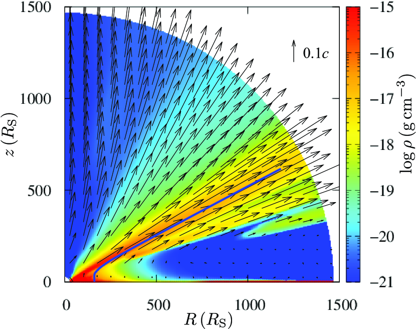
Figure 1: Time-averaged colour density map with the velocity vectors of the line-driven disc wind for $M_{\rm BH}=10^{8}\,M_{\odot}$, $\dot{m}_{\rm sup}=0.5$, and $f_{\rm X}=0.1$. The blue line shows a streamline through the mainstream (streamline passing through $\rho v_{r}$ peak at the outer boundary) of the wind. The $z=0$ plane roughly corresponds to the accretion disc surface and the $z$-axis is the rotational axis of the disc.

Fig. 2 shows the outflow properties at the outer boundary ($1500R_{\rm S}$) as a function of angle. The black solid line shows the result of the new simulation, where the mass accretion rate through the disc is reduced from $\dot{m}_{\rm sup}=0.5$ to $\dot{m}_{\rm BH}\sim 0.26$ at $R_{\rm launch}\sim 59R_{\rm S}$. This is compared to previous results with constant mass accretion rate through the disc (dashed lines) for $\dot{m}_{\rm sup}=0.5$ (blue) and $\dot{m}_{\rm sup}=0.2$ (red) that is close to the reduced $\dot{m}_{\rm BH}\sim 0.26$. Both the density and the velocity of the wind in the new simulation peak at an angle which is intermediate between the two constant mass accretion rate simulations (see top and bottom panels). The peak value of the wind density is close to that of $\dot{m}_{\rm sup}=0.5$. In contrast, the wind maximum velocity is close to the result of $\dot{m}_{\rm sup}=0.2$.

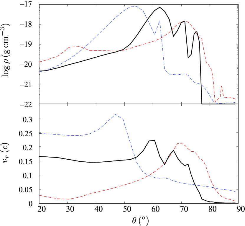
Figure 2: Angular profiles of the density (top panel) and the radial velocity (bottom panel) at the outer boundary ($r=1500R_{\rm S}$). The black solid lines show the profiles for the new mass-conserved simulations with $\dot{m}_{\rm sup}=0.5$ ($\dot{m}_{\rm BH}\sim 0.26$). The red dashed, and blue dashed lines show the profiles for the constant accretion rate models with $\dot{m}_{\rm sup}=0.2$, and $\dot{m}_{\rm sup}=0.5$.

The solid lines in Fig. 3 show the time-averaged density, velocity and optical depth along a streamline which goes through the peak wind momentum loss at the outer boundary (the blue line in Fig. 1). This streamline originates on the disc at $R\sim 160R_{\rm S}$, rises vertically upwards and then bends at height of $\sim 40R_{\rm S}$ to become a radial line, so all the vertical section of the streamline is at the same disc radius. The density (Fig. 3a) is high for the vertical section of the streamline (at constant disc radius with $R\sim R_{\rm min}\sim 160R_{\rm S}$), and only drops to become $\propto R^{-2}$ when the streamline bends. Most of the acceleration takes place in this vertical section, so the velocity increases rapidly at $R_{\rm min}$ (Fig. 3b, see also Fig. 4). There is also a slower acceleration zone where the wind velocity increases from $\sim\!0.1c$ to $\sim\!0.2c$ along the radial section of the streamline, from $R\gtrsim 160R_{\rm S}$. This is a consequence of the ionization, which is very low at these radii, with $\xi\sim 0$ so that UV line driving is very effective (see also Fig. 4). This low ionization parameter can be understood from the optical depth to X-rays, which is always larger than $\tau_{X}\sim 100$ (Fig. 3c), so the X-rays cannot penetrate into this section of the wind so the UV force multiplier is large.

We show details of the acceleration zone in our model in Fig. 4, again along the main streamline shown by the blue line in Fig. 1 but this time plotted against vertical position above the disc rather than radius. The streamline rises vertically from the disc, and bends radially at $z\sim 40R_{\rm S}$ (indicated by the vertical red dashed-dotted line). The velocity becomes supersonic near the disc surface ($z\sim 0.2R_{\rm S}$, see the black solid line in Fig. 4a compared to the horizontal solid blue line which marks $v=c_{\rm s}$) and becomes larger than the escape velocity at $z\sim 70R_{\rm S}$ where the matter is accelerated toward $r$-direction (the black dashed line in Fig. 4a compared to the horizontal blue dashed line which marks $v=v_{\rm esc}$). The dashed black line in Fig. 4b shows the ratio of radiation force to gravity in the $\theta$-direction. This exceeds unity close to the surface of the disc ($z\sim 0.1R_{\rm S}$). By contrast, the solid black line shows this ratio in the $r$-direction, $f_{{\rm rad},r}/g_{r}$. This only starts to become important around $z\sim 40R_{\rm S}$. These results mean that the matter is first vertically accelerated and becomes supersonic due to the radiation emitted from the disc right under the matter in the region of $z\lesssim 40R_{\rm S}$. At $z\sim 40R_{\rm S}$, the radiation pressure from the inner region also starts to become important. This changes the streamline trajectory to radial, but the material continues to accelerate as it still has substantial UV opacity so that the material reaches and exceeds the escape velocity. We show the ratio of $f_{{\rm rad,}r}/f_{{\rm rad},\theta}$ in Fig. 4c. This shows that the radial force becomes larger than the $\theta$-component at $z\sim 40R_{\rm S}$, changing the direction of the streamline. Fig. 4d indicates that the force multiplier becomes $\sim\!1$ at $z\sim 0.1R_{\rm S}$ and increases with the distance from the disc surface ($z=0$ plane). This means that the line force is comparable or larger than the radiation force due to the electron scattering in $z\gtrsim 0.1R_{\rm S}$. The main contributor to the acceleration of the wind is the line force, even after $z\sim 40R_{\rm S}$ where the radiation from the central disc and X-ray source are important.

However, this is a consequence of the assumption that the wind is highly optically thick to X-ray radiation, with X-ray optical depth $\tau_{\rm X}$ is equal to $100\tau_{\rm e}$ for $\xi\leq 10^{5}$. We can see explicitly the effect of this assumption on the ionization state by a comparison to the phenomenological biconical wind model of Hagino et al. (2015) designed to fit to the ultra-fast outflow in PDS456. This has an assumed (rather than calculated) velocity structure such that $v_{r}(l)=v_{0}+(v_{\infty}-v_{0})[1-R_{\rm min}/(R_{\rm min}+l)]$ where $v_{\infty}=0.237c$ (the dashed line in Fig. 3b), and an assumed (rather than calculated) geometry where $R_{\rm min}=10$–$15R_{\rm S}$ is the launch radius of the wind. Mass conservation then sets the density $\propto(v_{r}R^{2})^{-1}\to R^{-2}$ at large radii, and matches quite well to our hydrodynamical model results for $R\gtrsim 160R_{\rm S}$ (the dashed line in Fig. 3a). However, this has very different ionization structure with $\log\xi\sim 4$ which is much larger than the hydrodynamical results ($\xi\sim 0$). This is because this model assumes that $\tau_{\rm X}=\tau_{\rm e}$, so then the wind is never optically thick along this sightline and the X-ray flux remains high. We will explore this further with more realistic photoionization cross-sections for both the X-ray and line-driving fluxes in a future paper. Here we simply recognize that $\tau_{\rm X}=100\tau_{\rm e}$ for $\xi\leq 10^{5}$ and $\tau_{\rm X}=\tau_{\rm e}$ are opposite extreme assumptions, so we calculate the wind properties using both of these to understand the effect of photoionization on our wind.

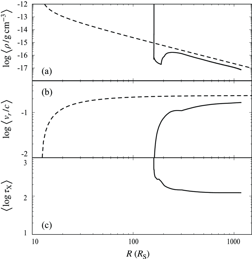
Figure 3: Density (panel a), velocity (panel b), and optical depth to the central X-ray source (panel c) along the streamline. The angle brackets denote the time-averaged values. The horizontal axis is the distance from the rotational axis of the disc. The solid lines show the results along the mainstream (blue line in Fig. 1) of our simulations for $M_{\rm BH}=10^{8}\,M_{\odot}$, $\dot{m}_{\rm sup}=0.5$, and $f_{\rm X}=0.1$. The dashed lines show the expectations from the phenomenological model of Hagino et al. (2015) with the wind terminal velocity of $v_{\infty}=0.237c$ and the mass loss rate of $8\,M_{\odot}{\rm yr^{-1}}$.

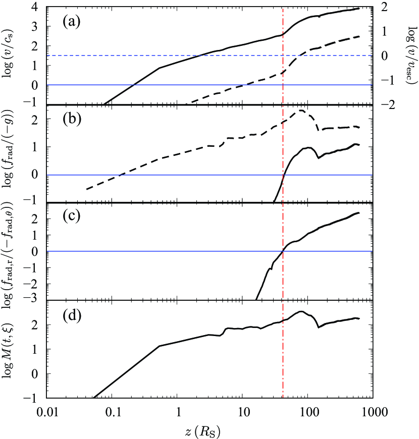
Figure 4: The velocity (panel a), the radiation force normalized by the gravity (panel b), the ratio of the $r$-component of the radiation force to the $\theta$-component (panel c), and the force multiplier (panel d) on the major wind streamline (blue line in Fig 1). The horizontal axis is the distance from the $z=0$ plane. In the panel a, the velocity is normalized by the sound speed (solid line) and by the escape velocity (dashed line). The solid line in the panel b shows the $r$-component of the radiation force, and the $\theta$-component is presented by the dashed line. The wind matter mainly moves vertically at $z\lesssim 40R_{\rm S}$ (left side of red dashed-dotted line), and is blown away in the radial direction at $z\gtrsim 40R_{\rm S}$ (right side of red dashed-dotted line).

3.2 Wind mass loss rate as a function of X-ray illumination

We now explore how the wind depends on the X-ray illumination. In our method, we ignore the scattered and reprocessed X-ray photons and assume that the X-ray is emitted from the point source. Although these assumptions are somewhat simpler to study the realistic dependence on the X-ray illiumination, following parameter survey helps us to understand the effect of the X-ray on the wind properties. Physically, we expect that the wind mass loss rate should depend on the strength of X-ray illumination as the X-rays overionize the wind, removing the UV opacity which is the driver for the wind launching mechanism. This causes the wind to fall back to the disc (failed wind) if it has not already reached its escape velocity at the point at which it becomes ionized (PK04; Risaliti & Elvis 2010; Nomura et al. 2013). The failed wind region creates a shadow which progressively shields the proto-wind at larger radii from the ionizing flux, so that eventually some material reaches the escape velocity and the wind is formed at larger radii. This predicts some correlation of the wind properties (increasing launch radius, decreasing velocity and decreasing mass loss rate) with increasing central X-ray illumination.

The strength of X-ray illumination at any given point will also have some dependence on the geometry of the central X-ray source. This is not well known at present, so we assume that the X-rays are from a compact central source, whose size is much smaller than the inner radius of our computational domain, $r_{\rm i}=30R_{\rm S}$. This is almost certainly not correct for the larger values of $f_{\rm X}$, but we neglect this here so as to be able to quantify the effect of a central X-ray source on the wind.

The filled circles in Fig. 5 show the wind outflow rates from our fiducial model with $M_{\rm BH}=10^{8}\,M_{\odot}$ and $\dot{m}_{\rm sup}=0.5$ for $f_{\rm X}=0$, 0.04 and 1 as well as our fiducial model with $f_{\rm X}=0.1$. There is indeed an anti-correlation of mass loss rate with increasing $f_{\rm X}$, but the effect is rather small, with only a factor 2 difference between no X-ray illumination ($f_{\rm X}=0$) and the model where the X-ray power is as strong as the total flux from the disc ($f_{\rm X}=1$, top panel). The wind launch radii are almost identical for all models, in fact slightly decreasing for the higher $f_{\rm X}$, contrary to the physical expectation that the requirement for increasing shielding with increasing $f_{\rm X}$ would mean that the wind is launched from further out (middle panel). The averaged radial wind velocity weighted by the density also shows the anti-correlation with increasing $f_{\rm X}$, but the effect is small (bottom panel).

Hence even intense X-ray illumination does not destroy the wind for this highly UV luminous disc (see also Fig. 7 and 8 in Nomura et al., 2016). However, the wind is strongly shielded from the central X-ray flux in part due to the assumption that $\tau_{\rm X}=100\tau_{\rm e}$ for $\xi\leq 10^{5}$. By comparison, the phenomenological biconical wind in Hagino et al. (2015) has $\xi\sim 10^{4}$ and its optical depth through the wind is $\tau_{\rm e}\sim 1$ at $76^{\circ}$ (see Fig. 3 in Hagino et al., 2015).

We assess the impact of the assumption that $\tau_{\rm X}=100\tau_{\rm e}$ for $\xi\leq 10^{5}$ by comparing this instead with $\tau_{\rm X}=\tau_{\rm e}$. PK04 also explore this possibility, coupled with assuming that the UV optical depth is zero rather than $\tau_{\rm UV}=\tau_{e}$. We follow their combination of $\tau_{\rm X}$ and $\tau_{\rm UV}$ assumptions so we can compare results. Fig. 5 (open circles) shows the wind properties with these different assumed X-ray and UV optical depths. The wind is similar for $f_{\rm X}=0$. There is a steeper drop in the wind loss rate for $f_{\rm X}=0$ to $0.04$ (top panel), and a sharp increase in wind launch radius (middle panel) as expected due to the wind being more ionized. However, there is still a strong wind, even at $f_{\rm X}=1$, with mass loss rates across the range of X-ray flux which are a factor $\sim\!2$–4 times smaller than those of our fiducial model (filled circles). There is enough shielding even for high X-ray luminosity since it only requires $\tau_{\rm e}>1$ to reduce the X-ray ionizing flux substantially. We will explore how robust our result is to a more detailed photoionization model in a subsequent paper.

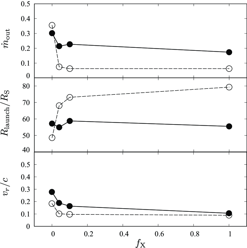
Figure 5: Wind mass loss rate (top panel), launching radius (middle panel), and averaged radial velocity weighted by the density (bottom panel) as functions of X-ray fraction, $f_{\rm X}$. We employ $M_{\rm BH}=10^{8}\,M_{\odot}$ and $\dot{m}_{\rm sup}=0.5$ for $f_{\rm X}=0$, 0.04, 0.1 and 1. The filled circles show the results when we employ $\sigma_{\rm X}=\sigma_{\rm e}$ for $\xi>10^{5}$ and $100\sigma_{\rm X}$ for $\xi\leq 10^{5}$. The open circles indicate the results using $\sigma_{\rm X}=\sigma_{\rm e}$ independently of $\xi$ and ignoring the attenuation of the UV line-driving flux.

3.3 Wind mass loss rate as a function of $\dot{m}_{\rm sup}$ for realistic AGN SEDs

Fig. 6a shows the effect of changing the black hole Eddington fraction, for $\dot{m}_{\rm sup}=0.1,0.5$ and $0.9$. We do this for fixed $M_{\rm BH}=10^{8}\,M_{\odot}$ and $f_{\rm X}=0.1$, and also for a probably more realistic AGN SED model where $f_{\rm X}$ decreases as $\dot{m}_{\rm sup}$ increases (Done et al., 2012; Jin et al., 2012). Kubota & Done (2018) show that assuming $L_{\rm X}=f_{\rm X}L_{\rm D}=0.02L_{\rm Edd}$ gives a fairly good match to the observed data, so we also repeat the calculations for $f_{\rm X}=0.2$ for $\dot{m}_{\rm sup}=0.1$, 0.04 for $\dot{m}_{\rm sup}=0.5$ and $0.02$ for $\dot{m}_{\rm sup}=0.9$. However, as explained above, the hard X-rays make very little difference to the wind properties in these simulations so the results are very similar to those with fixed $f_{\rm X}$ so we only show one set of results here.

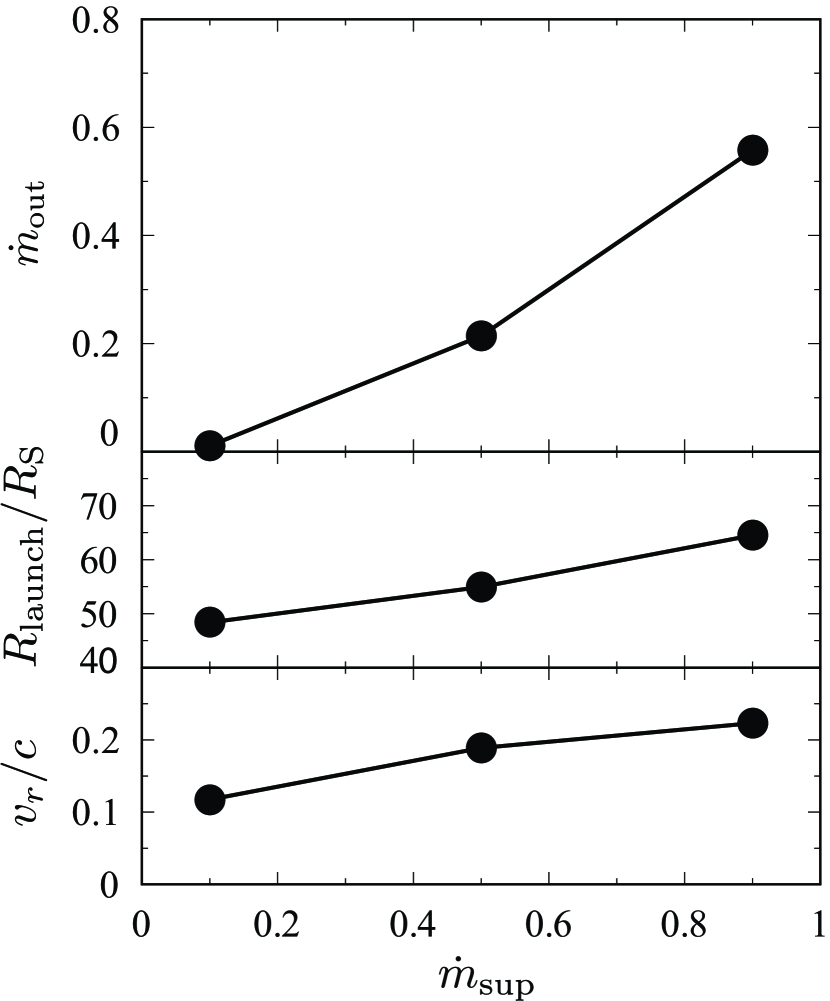
Figure 6: Wind mass loss rate (panel a), launching radius (panel b), and averaged radial velocity weighted by the density (bottom panel c) as functions the mass supply rate. The black hole mass and the X-ray fraction are $M_{\rm BH}=10^{8}\,M_{\odot}$ and $f_{\rm X}=0.2,0.04,0.02$ for $\dot{m}=0.1,0.5,0.9$.

As expected, the mass outflow rates in the wind increase for increasing $\dot{m}_{\rm sup}$, with $\dot{m}_{\rm out}=1.1\times 10^{-2}$, $0.21$ and $0.56$ for $\dot{m}_{\rm sup}=0.1$, $0.5$, and $0.9$, which correspond to $11\%$, $42\%$ and $62\%$ of the mass supply rates. The wind efficiency is a strong function of $\dot{m}_{\rm sup}$, and powerful UV line-driven winds are not produced in our code below $\dot{m}_{\rm sup}\sim 0.1$–$0.2$. Fig. 6b shows the launch radius increases with $\dot{m}_{\rm sup}$, as expected as the UV bright section of the disc is characterized by a constant temperature of $\sim\!50,000\,$K and this moves outwards with increasing $\dot{m}_{\rm sup}$. The wind velocity slightly increases with $\dot{m}_{\rm sup}$ (Fig. 6c). The outward shift of the UV zone caused by the large accretion rate tends to decrease the wind velocity since the escape velocity decreases with an increase of the radius. However, the larger mass accretion rate, the larger line-driving luminosity. Thus, the wind velocity is thought to gradually rise with accretion rate.

Fig. 7 shows the resulting SED from the underlying disc emission for the $10^{8}\,M_{\odot}$ case. The strong wind losses for $\dot{m}_{\rm sup}=0.9$ means that most of the accretion power is released as kinetic luminosity rather than radiation, and the SED is much redder than expected from a pure disc model. By contrast, the small wind losses at $\dot{m}_{\rm sup}=0.1$ mean that the mass accretion rate through the disc is not so different between the inner and outer regions, so it looks almost like a standard disc.

These spectra look very like the variable mass accretion rate disc spectra predicted by Laor & Davis (2014) which used O star winds to characterize the mass loss rate from each radius of the disc. Their models assumed that there was no central X-ray source, so have maximal wind mass loss rates. They reran their code for the specific case of $M_{\rm BH}=10^{8}\,M_{\odot}$ and $\dot{m}_{\rm sup}=0.1$ so we could directly compare. Their model had a powerful mass outflow, such that $\dot{m}_{\rm BH}\sim 0.02$ (0.05) if none (all) of the material lost in the wind reaches the local escape velocity. However, this wind is launched at $15R_{\rm S}$, which is below our hydrodynamic inner grid limit of $30R_{\rm S}$. Thus our calculations cannot test whether such a wind is present.

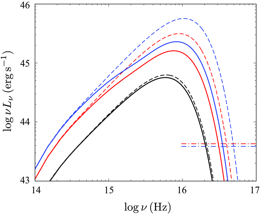
Figure 7: SEDs of the radiation from the accretion discs when we set $M_{\rm BH}=10^{8}\,M_{\odot}$. The black, red, and blue solid lines show the SEDs for $\dot{m}_{\rm sup}=0.1$, $0.5$, and $0.9$ of our mass-conserved simulations. The black, red, and blue dashed lines are the SEDs of the standard disc model with $\dot{m}_{\rm sup}=0.1$, $0.5$, and $0.9$. The black, red, and blue dot-dashed lines are the X-ray spectra employing the power-law spectrum with a photon index of $\Gamma=2$. The X-ray fractions are $f_{\rm X}=0.2$, 0.04, and 0.02 for $\dot{m}_{\rm sup}=0.1$, 0.5, and 0.9.

4 Discussion

4.1 AGN feedback

We present the first radiation hydrodynamic simulations of UV line-driven disc winds which adjust the underlying disc emission to compensate for the mass loss rates in the wind. This is extremely important as previous calculations have inferred mass outflow rates which are larger than the mass supply rate at the moderately high Eddington ratios $\dot{m}_{\rm sup}\sim 0.5$. The most powerful winds in the local Universe are seen in similarly high $\dot{m}_{\rm sup}$ rates ($\sim\!0.5$ and above), e.g., PDS456 (Reeves et al., 2009) and PG1211 (Pounds et al., 2003), so these sources could not be well modeled in previous work. These are the sources where the winds have enough power to affect star formation in the bulge of the host galaxy. Our new results show that while the wind power is reduced from previous studies (N17), the winds are still powerful. We evaluate the kinetic luminosities of the winds by integrating over the outer boundary, so $L_{\rm kin}=2\pi r^{2}\int^{89^{\circ}}_{0}\rho v_{r}^{3}\sin\theta d\theta$ giving $\sim\!4\%$, $\sim\!25\%$, and $\sim\!33\%$ of the disc luminosity for $\dot{m}_{\rm sup}=0.1$, $0.5$, and $0.9$ when the black hole mass is $M_{\rm BH}=10^{8}\,M_{\odot}$. These results are consistent with those estimated from the X-ray observations (Tombesi et al., 2012a; Gofford et al., 2015). The model proposed by Di Matteo et al. (2005) suggests that the required kinetic luminosity for the feedback is at least 5% of the bolometric luminosity, although Hopkins & Elvis (2010) reduce the criteria down to 0.5% based on the simulations focusing on a cloud in the interstellar medium exposed to the radiation and diffuse outflow from the AGN. Ostriker et al. (2010) performed large-scale one- and two-dimensional calculations and found that winds can affect the surrounding environment even if the kinetic luminosity is less than $\sim 10^{-4}\dot{M}_{\rm acc}c^{2}$, which is not inconsistent with the estimation by Hopkins & Elvis (2010).

In addition to the mechanical feedback via the winds, the radiative feedback would be also important for the large-scale inflow and outflow (e.g., Kurosawa & Proga, 2009). Cosmological zoom-in simulations with the mechanical feedback via the winds and the radiative feedback using the simplified AGN feedback model are rapidly developed (e.g., Choi et al., 2017; Brennan et al., 2018). Our present model can give the mechanical and radiative feedbacks quantitatively, since the wind power and the disc luminosity are calculated as functions of the mass supply rate and the black hole mass.

4.2 Limitations of current model and future works

There are several limitations of the current code, which are inherent in the current ‘standard’ setup of hydrodynamics and radiation transfer for UV line-driven disc wind simulations. We highlight the limitations of the radiative transfer, in particular the abrupt switch from $\sigma_{\rm X}=\sigma_{\rm e}$ to $100\sigma_{\rm e}$ at $\xi<10^{5}$ which means that the X-rays are heavily attenuated below this ionization parameter. This is a drastic overestimate of the opacity for material with $10^{3}\lesssim\xi\lesssim 10^{5}$, which leads to the very efficient shielding. Hence the effect of X-ray illumination on the wind structure is almost certainly underestimated in these calculations. In the case of line-driving UV radiation, the opacity is assumed to be simply $\sigma_{\rm e}$, which would underestimate the attenuation of the UV flux for $\xi\lesssim 10$. This treatment is physically inconsistent with that the UV radiation is absorbed by the wind material through the bound-bound transitions. The model also does not include the ionizing effect of the disc photons above 200 Å, which will be substantial especially for the hotter discs predicted for smaller black hole masses and higher mass accretion rates. We will explore more physical models of X-ray and UV opacity in future work.

Additionally, we ignore the scattered and reprocessed photons for simplicity in our method. However, postprocessed radiation transfer calculations suggest that these secondary photons ionize the wind materials (Sim et al., 2010; Higginbottom et al., 2014). This might affect the line-driving mechanism and the resulting mass loss rate of the disc wind. Higginbottom et al. (2014) performed Monte Carlo simulation of the radiative transfer through the results of PK04. They found that the ionization parameter estimated by Monte Carlo simulation including the secondary photons is $\sim\!4$ orders of magnitude larger than that from PK04 in the outflowing material, though the ionization parameters are not so different in the high-density region ($\gtrsim\!10^{14}\,{\rm g\,cm^{-3}}$). The increase of the ionization parameter would weaken the line driving and reduce the mass outflow rate. In order to quantitively assess the effect due to the secondary radiation, the hydrodynamics simulations coupled with the radiation transfer considering scattered and reprocessed photons are necessary. Such simulations are not realistic due to the large computational costs at this time, but the improvement of treatment of radiation transfer is an important future work in this field.

The computational domain is fixed from $30$–$1500R_{\rm S}$, yet physically it would be better for this to adapt in size to cover the disc UV temperature zone for the given black hole mass and mass accretion rate. The temperature in a standard disc is $T^{4}\propto\dot{m}_{\rm sup}/M_{\rm BH}r^{3}$, and the UV zone extend inwards of $30R_{\rm S}$ for our lowest $\dot{m}_{\rm sup}=0.1$ case. Including these inner radii would also enable us to test the Laor & Davis (2014) UV line-driven disc wind models based on O star winds, and would allow us to calculate the wind mass loss rates for higher mass black holes, where the disc temperature is lower so the UV zone is at smaller radius and again extends below our fixed inner radius. However, our disc does not have constant mass accretion rate, and the inner radii have lower temperature than predicted due to the mass loss rate in the wind. At radii smaller than the wind launch radius the disc temperature is lower, $T^{4}\propto\dot{m}_{\rm BH}/M_{\rm BH}r^{3}$. Hence the computational domain should extend inwards of the initial predicted UV zone in order that it can properly capture the wind launch even after its temperature is adjusted for the mass loss rate. Just extending the grid inwards would mean that there are larger number of time-integration steps (caused by smaller grid spacing) and more grid points for the hydrodynamic calculation, which would slow the code down considerably. However, the outer disc in AGN should become self gravitating at a radius of only a few hundred $R_{\rm S}$, so shifting the same number of grid points inwards, which somewhat reduces computational costs, gives a much more physically realistic disc wind simulation. However shifting the computational domain inwards means that the X-ray illumination then depends on the unknown X-ray source geometry. Intriguingly, one potential source geometry is that the hard X-rays are powered by the mass accretion flow, so that the energy at small radii is dissipated in X-ray hot, optically thin plasma rather than in the optically thick disc (Done et al., 2012; Kubota & Done, 2018). We will explore the effect of this and other potential source geometries.

Our code considers the reduction of the mass accretion rate caused by the wind but does not solve the structure of the accretion disc itself. In order to obtain fully self-consistent results, it is necessary to perform the multidimensional simulations of the wind and the disc structure. In the current method, we assume that the geometrically thin and optically thick disc lies below the computational domain. The boundary at $\theta=\pi/2$ corresponds to the disc surface. When we estimate the line-driving flux, the disc is treated as an external radiation source and the photons are supposed to be steadily emitted from the vicinity of the equatorial plane of the disc. Although the line force was not considered, global two-dimensional radiation hydrodynamics/magnetohydrodynamics simulations of the standard disc and the wind were performed by Ohsuga (2006), Ohsuga et al. (2009) and Ohsuga & Mineshige (2011).

Despite all these caveats, our model is the first hydrodynamic code to include the response of the disc to the mass loss rate in the line-driven wind. We show that the resulting continuum spectra are different from those of the standard discs when the line-driven winds are launched (Fig. 7), similar to the numerical models of the disc structure based on O star wind mass loss rates by (Laor & Davis, 2014). The resulting spectrum should also be absorbed by the wind material along lines of sight which intersect the mass outflow, so blueshifted absorption lines should be superimposed on the spectra. More detailed spectral models should include radiation transfer through this material, as have been done for the models of PK04 by Schurch et al. (2009); Sim et al. (2010); Higginbottom et al. (2014).

The time variation of the absorption lines (e.g., Misawa et al., 2007; Tombesi et al., 2012b) is the remaining problem. This implies that the disc wind changes its structure in time and/or has non-axisymmetric clumpy structure. The density fluctuations of line-driven winds are found in one- or two-dimensional calculations (Owocki & Puls, 1999; Proga et al., 2000). In addition, recently, three-dimensional simulations of line-driven winds for cataclysmic variables reported the non-axisymmetric structure of the winds (Dyda & Proga, 2018a, b). Application of the three-dimensional calculations to AGNs and investigate the origin of the time variation are the important future works.

Although we focus on the sub-Eddington sources in the present work, we need to investigate the super-Eddington cases in order to resolve the role of the outflow in the evolution of the most rapidly growing SMBHs. Radiation hydrodynamics simulations of super-Eddington sources revealed that radiation pressure on electrons accelerates the winds from the accretion discs (e.g., Ohsuga et al., 2009; Ohsuga & Mineshige, 2011; Takeuchi et al., 2013; Kobayashi et al., 2018). UV line driving would assist in launching disc winds as the luminosity approaches and then exceeds Eddington so that the radiation hydrodynamics simulations considering a combination of radiation pressure on electrons and the UV line driving are important for super-Eddington accretion flows. Such simulations are left as future work.

5 Conclusions

By performing the two-dimensional radiation hydrodynamics simulations, we found that the line-driven winds suppress the mass accretion onto the black hole especially in the luminous AGNs ($\dot{m}_{\rm sup}\gtrsim 0.5$). Our simulations are the first mass-conserved hydrodynamic models to include the reduction of the mass accretion rate through the inner disc due to the launching of disc winds.

We show results for a black hole mass of $M_{\rm BH}=10^{8}\,M_{\odot}$, with mass supply rates of $\dot{m}_{\rm sup}=0.1$, $0.5$, and $0.9$. We find a powerful wind is generated in the latter two models, and the kinetic power of these winds is around 25% of the disc luminosity, which is sufficient for AGN feedback (Di Matteo et al., 2005; Hopkins & Elvis, 2010).

The wind mass loss rate suppresses the mass accretion rate after the launching radius of the wind, producing a different accretion disc continuum spectra which shows reduced flux in the UV ($\nu\gtrsim 10^{15}\,{\rm Hz}$) due to the large suppression of the mass accretion rate and corresponding low effective temperature in the inner disc. For $\dot{m}_{\rm sup}\gtrsim 0.5$, there is clear difference between the SEDs predicted by our simulations and the SEDs assuming the constant accretion rate. This indicates that the line-driven wind imprints an observable feature into the continuum spectra, which may corresponds to a observed turnover in the UV at a constant temperature, modeled by Laor & Davis (2014) using analytic/numerical calculations based on O star winds.

Our calculations here show the feasibility of producing a quantitative model for AGN feedback via UV line-driven winds. We highlight a number of issues with the standard hydrodynamical disc wind setup which currently limit the reliability of these models, but we will address these in a subsequent paper and apply the model to sources in the wide range of the black hole mass and the mass accretion rate. This would enable us to quantify the AGN feedback via winds across cosmic time.

Appendix A Comparison with previous works

A.1 Force multiplier

The force multiplier in our simulations is consistent with the solution of Castor et al. (1975, hereafter CAK75) that is the one-dimensional line-driven stellar wind model. Fig. 8 in CAK75 shows that the force multiplier is $\sim\!2$–5 near the sonic point. Our result also indicates that the force multiplier is a few at the sonic point (where $v=c_{\rm s}$, $z\sim 0.07R_{\rm S}$) on the major wind streamline (see Fig. 4d).

Fig. 4d also shows the force multiplier in our model increases with the distances and reaches $\sim\!100$ at the point far away from the disc. The increase of the force multiplier also occurs in CAK75, in which the force multiplier goes up with an increase of the distances from the photosphere. However, the force multiplier in the present model ($\sim\!100$) is much larger than that of CAK75 ($\sim\!$ a few). The enhancement of the force multiplier is caused by the reduction of the local optical depth parameter, which is proportional to the density and inverse proportional to the velocity gradient (see Eq. 13). The velocity gradient of our model is $\sim\!10^{-4}c/R_{\rm S}$ –$10^{-3}c/R_{\rm S}$ since the wind is still slowly accelerated at the point far away from the disc (Fig. 3b). In contrast, the velocity gradient is very small in CAK75 since the wind almost reaches the terminal velocity. In addition, the density in our model decreases with an increase of the distance more rapidly than in CAK75 model. These density and velocity features cause the small local optical depth parameter and the larger force multiplier.

The force multiplier continually increases for $R\gtrsim 100$, but the total line force is the product of this with the line-driving flux which roughly $\propto R^{-2}$. Hence the total line force contributes most in the inner region ($R\sim 100R_{\rm S}$ and $z\lesssim 30R_{\rm S}$ for the major streamline).

Our simple method for evaluation of the velocity gradient ($dv/ds$) does not lead to a large error in the force multiplier. As we have mentioned in Section 2.2, we evaluate $dv/ds$ along the direction of the line-driving flux in order to suppress the computational cost. However, strictly speaking, $dv/ds$ should be calculated along each light-ray. Therefore, an ideal manner is calculating $dv/ds$ along the numerous light-rays from the disc surface and evaluating the direction-dependent force multiplier.

In order to compare between our present method and more accurate method, we perform the test calculation where we calculate $dv/ds$ along the $4096\times 4096$ light-rays and estimate the force multiplier and line force (This method is similar to that of PK04 but they prepare $12\times 12$ light-rays). Here, we use the velocity distribution of a snapshot of our simulations for $M_{\rm BH}=10^{8}M_{\odot}$ and $\dot{m}_{\rm sup}=0.5$.

As a result, we confirm that the line force estimated by our current method is quite similar to that of the test calculation. At the point on the major wind streamline, where the matter is effectively accelerated in the vertical direction ($R\sim 100R_{\rm S}$ and $z\sim 0.2R_{\rm S}$), the $\theta$-component of the line force is $f_{{\rm line},\theta}\sim-11.5\times 10^{-7}c^{2}/R_{\rm S}$ for our method and $\sim\!-8.6\times 10^{-7}c^{2}/R_{\rm S}$ for the test calculation. The force multiplier in the present method, $\sim\!1.9$, is roughly consistent with the $\theta$-component of the force multiplier, $M_{\theta}=cf_{{\rm line},\theta}/\sigma_{\rm e}F_{{\rm line},\theta}\sim 1.2$, for the test calculation. In both methods, the $r$-component of the line force is negligibly small compared to the $\theta$-component because the $r$-component of the line-driving flux is quite small.

At the point where the outflow velocity exceeds the escape velocity ($R\sim 140R_{\rm S}$ and $z\sim 60R_{\rm S}$), our present method gives $\left|f_{\rm line}\right|\sim 7.5\times 10^{-5}c^{2}/R_{\rm S}$, which is almost the same as the line force obtained by the test calculation, $\left|f_{\rm line}\right|\sim\!6.8\times 10^{-5}c^{2}/R_{\rm S}$. The force multiplier, $\sim\!50$, is also quite similar to that obtained from the test calculation, $M_{r}=cf_{{\rm line},r}/\sigma_{\rm e}F_{{\rm line},r}\sim 44$ and $M_{\theta}\sim 45$. These results show that our evaluation method for $dv/ds$ is reasonable. More accurate results would be obtained by the radiation hydrodynamics simulations in which the radiation transfer equations are solved along the many light-rays (Jiang et al., 2014; Ohsuga & Takahashi, 2016).

A.2 Effective temperature of accretion disc and opacities

Besides the method for estimation of $dv/ds$, the effective temperature of the disc and opacities in our simulations are different from those of PK04.

In our method, the X-ray opacity is set to be $\sigma_{\rm X}=100\sigma_{\rm e}$ for $\xi\leq 10^{5}$ or $\sigma_{\rm X}=\sigma_{\rm e}$ for $\xi>10^{5}$, and the $r$-component of line-driving flux is attenuated by supposing the opacity of $\sigma_{\rm UV}=\sigma_{\rm e}$ (see also Proga et al., 2000). In contrast, $\sigma_{\rm X}$ is set to be $\sigma_{\rm e}$ independently of $\xi$ and $\sigma_{\rm UV}$ is assumed to be null in PK04. As we explained in Sections 3.2, our treatment about $\sigma_{\rm X}$ leads the massive and fast wind (see Fig. 5) compared with the method of PK04. Since neither our method nor method in PK04 is rigid, hydrodynamics simulations coupled with the frequency-dependent radiation transfer calculations are needed in order to obtain more realistic winds.

Next, we consider the impact of the setting of the effective temperature. We use the simple radial profile of

$$T_{\rm eff}\left(r\right)=T_{\rm in}\left(\frac{r}{3R_{\rm S}}\right)^{-\frac{3}{4}}.$$ (20)

We set $T_{\rm in}$ to meet the condition of

$$\dot{m}_{\rm sup}L_{\rm Edd}=\int_{\rm 3R_{\rm S}}^{r_{\rm out}}4\pi r\sigma T_{\rm eff}^{4}dr,$$ (21)

where we suppose $T_{\rm eff}\left(r_{\rm out}\right)=3\times 10^{3}\,{\rm K}$ and $\sigma$ is the Stefan-Boltzmann coefficient. In contrast, PK04 employ

$$T_{\rm eff}\left(r\right)=T_{\rm in}\left(\frac{r}{3R_{\rm S}}\right)^{-\frac{3}{4}}\left(1-\sqrt{\frac{3R_{\rm S}}{r}}\right)^{\frac{1}{4}},$$ (22)

where

$$T_{\rm in}=\frac{3GM_{\rm BH}\dot{M}_{\rm sup}}{8\pi\sigma\left(3R_{\rm S}\right)^{3}}.$$ (23)

Although we consider the disc emission from the regions of $3R_{\rm S}\lesssim r\lesssim r_{\rm out}$, PK04 ignore the radiation from the inner part of the disc, $3R_{\rm S}\leq r<30R_{\rm S}$, where $T_{\rm eff}$ is $\gtrsim 5\times 10^{4}\,{\rm K}$.

Here, we perform two test runs: (A) employing our current $T_{\rm eff}(r)$ and (B) employing $T_{\rm eff}(r)$ described by PK04. In these tests, we employ $M_{\rm BH}=10^{8}\,M_{\odot}$, $f_{\rm X}=0.1$, and $\dot{m}_{\rm sup}=\dot{m}_{\rm BH}=0.5$. Also, we set $\sigma_{\rm X}=\sigma_{\rm e}$ and $\sigma_{\rm UV}=0$ same as PK04. The decreasing of the mass accretion due to the launching of the wind is not taken into consideration in the test runs. The results show that the mass loss rate estimated from the test run B is $\sim\!4.9$ times larger than that obtained from the test run A. The averaged radial velocity for the test run B ($v_{r}\sim 0.07c$), which is consistent with that of PK04 ($v_{r}\sim\!0.067c$), is almost the same as that of test run A ($v_{r}\sim 0.096c$).

The difference of the mass loss rate is understood as follows. The line-driving luminosity (the luminosity integrated by the wavelength across the UV transition of 200–3200 Å, see also Section 2.2) emitted from the base of the wind ($r\geq 30R_{\rm S}$) is $3.9\times 10^{44}\,{\rm erg\,s^{-1}}$ for the run A and $1.9\times 10^{45}\,{\rm erg\,s^{-1}}$ for the run B. Therefore, the matter near the disc surface would be effectively lifted up in the run B, leading to the larger mass loss rate. Although the mass loss rate mainly depends on the line-driving luminosity of the wind base ($r\geq 30R_{\rm S}$), the radial velocity of the wind would be determined by the total line-driving luminosity. For the run A, the total line-driving luminosity is $5.1\times 10^{45}\,{\rm erg\,s^{-1}}$. This is comparable to the the line-driving luminosity for the run B, $1.9\times 10^{45}\,{\rm erg\,s^{-1}}$. Note that the disc emission within $r<30R_{\rm S}$ is neglected in the run B, so that the line-driving luminosity of the wind base equals to the total line-driving luminosity. Since the efficiency of the acceleration in the radial direction of the wind is thought to depend on the total line-driving luminosity, the outflow velocity would become the same order in both runs.

To sum up, our simple treatment for the calculation of $dv/ds$ does not affect the results. Our assumption of $T_{\rm eff}\left(r\right)$ tends to suppress the wind mass loss but does not change the wind velocity. The opacities employed in the present simulations drastically enhance the wind power. Hence, the reason why the wind velocity is higher for the present simulations than for the PK04 would be mainly caused by the difference of the opacities. The detailed comparison among the various models is left as future work. Numerical simulations employing realistic effective temperature profile with a detailed photoionization model are also important future works.

References

- Blandford & Payne (1982) Blandford, R. D., & Payne, D. G. 1982, MNRAS, 199, 883
- Blondin (1994) Blondin, J. M. 1994, ApJ, 435, 756
- Brennan et al. (2018) Brennan, R., Choi, E., Somerville, R. S., et al. 2018, ApJ, 860, 14
- Chartas et al. (2002) Chartas, G., Brandt, W. N., Gallagher, S. C., & Garmire, G. P. 2002, ApJ, 579, 169
- Choi et al. (2017) Choi, E., Ostriker, J. P., Naab, T., et al. 2017, ApJ, 844, 31
- Castor et al. (1975) Castor, J. I., Abbott, D. C., & Klein, R. I. 1975, ApJ, 195, 157
- Di Matteo et al. (2005) Di Matteo, T., Springel, V., & Hernquist, L. 2005, Nature, 433, 604
- Done et al. (2012) Done, C., Davis, S. W., Jin, C., Blaes, O., & Ward, M. 2012, MNRAS, 420, 1848
- Dyda & Proga (2018a) Dyda, S., & Proga, D. 2018, MNRAS, 475, 3786
- Dyda & Proga (2018b) Dyda, S., & Proga, D. 2018, MNRAS, 478, 5006
- Ferrarese & Merritt (2000) Ferrarese, L., & Merritt, D. 2000, ApJ, 539, L9
- Fukumura et al. (2015) Fukumura, K., Tombesi, F., Kazanas, D., et al. 2015, ApJ, 805, 17
- Gofford et al. (2013) Gofford, J., Reeves, J. N., Tombesi, F., et al. 2013, MNRAS, 430, 60
- Gofford et al. (2015) Gofford, J., Reeves, J. N., McLaughlin, D. E., et al. 2015, MNRAS, 451, 4169
- Gebhardt et al. (2000) Gebhardt, K., Bender, R., Bower, G., et al. 2000, ApJ, 539, L13
- Hagino et al. (2015) Hagino, K., Odaka, H., Done, C., et al. 2015, MNRAS, 446, 663
- Higginbottom et al. (2014) Higginbottom, N., Proga, D., Knigge, C., et al. 2014, ApJ, 789, 19
- Hopkins & Elvis (2010) Hopkins, P. F., & Elvis, M. 2010, MNRAS, 401, 7
- Jiang et al. (2014) Jiang, Y.-F., Stone, J. M., & Davis, S. W. 2014, ApJS, 213, 7
- Jin et al. (2012) Jin, C., Ward, M., & Done, C. 2012, MNRAS, 422, 3268
- King (2003) King, A. 2003, ApJ, 596, L27
- Kobayashi et al. (2018) Kobayashi, H., Ohsuga, K., Takahashi, H. R., et al. 2018, PASJ, 70, 22
- Konigl & Kartje (1994) Konigl, A., & Kartje, J. F. 1994, ApJ, 434, 446
- Kubota & Done (2018) Kubota, A., & Done, C. 2018, MNRAS, 480, 1247
- Kurosawa & Proga (2009) Kurosawa, R., & Proga, D. 2009, MNRAS, 397, 1791
- Laor & Davis (2014) Laor, A., & Davis, S. W. 2014, MNRAS, 438, 3024
- Magorrian et al. (1998) Magorrian, J., Tremaine, S., Richstone, D., et al. 1998, AJ, 115, 2285
- Misawa et al. (2007) Misawa, T., Eracleous, M., Charlton, J. C., & Kashikawa, N. 2007, ApJ, 660, 152
- Murray et al. (1995) Murray, N., Chiang, J., Grossman, S. A., & Voit, G. M. 1995, ApJ, 451, 498
- Nomura et al. (2013) Nomura, M., Ohsuga, K., Wada, K., Susa, H., & Misawa, T. 2013, PASJ, 65, 40
- Nomura et al. (2016) Nomura, M., Ohsuga, K., Takahashi, H. R., Wada, K., & Yoshida, T. 2016, PASJ, 68, 16
- Nomura & Ohsuga (2017) Nomura, M., & Ohsuga, K. 2017, MNRAS, 465, 2873
- Ohsuga (2006) Ohsuga, K. 2006, ApJ, 640, 923
- Ohsuga et al. (2009) Ohsuga, K., Mineshige, S., Mori, M., & Kato, Y. 2009, PASJ, 61, L7
- Ohsuga & Mineshige (2011) Ohsuga, K., & Mineshige, S. 2011, ApJ, 736, 2
- Ostriker et al. (2010) Ostriker, J. P., Choi, E., Ciotti, L., Novak, G. S., & Proga, D. 2010, ApJ, 722, 642
- Ohsuga & Takahashi (2016) Ohsuga, K., & Takahashi, H. R. 2016, ApJ, 818, 162
- Owocki & Puls (1999) Owocki, S. P., & Puls, J. 1999, ApJ, 510, 355
- Pounds et al. (2003) Pounds, K. A., Reeves, J. N., King, A. R., et al. 2003, MNRAS, 345, 705
- Proga et al. (2000) Proga, D., Stone, J. M., & Kallman, T. R. 2000, ApJ, 543, 686
- Proga & Kallman (2004) Proga, D., & Kallman, T. R. 2004, ApJ, 616, 688
- Reeves et al. (2003) Reeves, J. N., O’Brien, P. T., & Ward, M. J. 2003, ApJ, 593, L65
- Reeves et al. (2009) Reeves, J. N., O’Brien, P. T., Braito, V., et al. 2009, ApJ, 701, 493
- Risaliti & Elvis (2010) Risaliti, G., & Elvis, M. 2010, A&A, 516, 89
- Shakura & Sunyaev (1973) Shakura, N. I., & Sunyaev, R. A. 1973, A&A, 24, 337
- Schurch et al. (2009) Schurch, N. J., Done, C., & Proga, D. 2009, ApJ, 694, 1
- Shields et al. (1986) Shields, G. A., McKee, C. F., Lin, D. N. C., & Begelman, M. C. 1986, ApJ, 306, 90
- Sim et al. (2010) Sim, S. A., Proga, D., Miller, L., Long, K. S., & Turner, T. J. 2010, MNRAS, 408, 1396
- Stevens & Kallman (1990) Stevens,I. R., & Kallman, T. R. 1990, ApJ, 436, 599
- Takeuchi et al. (2013) Takeuchi, S., Ohsuga, K., & Mineshige, S. 2013, PASJ, 65, 88
- Tombesi et al. (2010) Tombesi, F., Cappi, M., Reeves, J. N., et al. 2010, A&A, 521, A57
- Tombesi et al. (2011) Tombesi, F., Cappi, M., Reeves, J. N., et al. 2011, ApJ, 742, 44
- Tombesi et al. (2012a) Tombesi, F., Cappi, M., Reeves, J. N., & Braito, V. 2012, MNRAS, 422, L1
- Tombesi et al. (2012b) Tombesi, F., Sambruna, R. M., Marscher, A. P., et al. 2012, MNRAS, 424, 754
- Tremaine et al. (2002) Tremaine, S., Gebhardt, K., Bender, R., et al. 2002, ApJ, 574, 740