Primordial Lithium Puzzle and the Axion Quark Nugget Dark Matter Model

Abstract

Astrophysics today faces a number of mysteries which defiant their resolutions in spite of drastic improvements in instrumental design, better technique being developed, and gradual improvements in theoretical and computation methods over last decades. Primordial Lithium Puzzle is known to stay with us for at least two decades, and it is very likely that its final resolution will require some fundamentally new ideas, novel frameworks and a non-conventional paradigms. We propose that Primordial Lithium Puzzle finds its natural resolution within the so-called Axion Quark Nugget (AQN) dark matter model. This model was invented long ago as a natural explanation of the observed ratio $\Omega_{\rm dark}\sim\Omega_{\rm visible}$ without any references to BBN physics. In this new paradigm, in contrast with conventional WIMP (Weakly Interacting Massive Particle) framework the dark matter (DM) takes the form of the macroscopically large quark nuggets without requiring any new fields beyond the standard model physics, except for the axion. The time evolution of these AQNs in primordial soup at $T\sim 20$ KeV suggests a strong suppression of the abundances of nuclei with high charges $Z\geq 3$. This suppression mechanism represents the resolution of the primordial lithium abundance within AQN dark matter scenario.

I Introduction

Prediction of the primordial abundances of light elements during the Big Bang Nucleosyntheis (BBN) is one of the major triumphs of physics and cosmology. Indeed, the BBN theory has no free parameters to fit the data (if the barion-to-photon ratio $\eta$ is taken from the Cosmic Microwave Background data). In spite of the complexity of many coupled nuclear reactions during BBN the abundances of helium and deuterium (which differs by 4 orders of magnitude) are predicted with high accuracy. The only remaining problem is the abundance of ⁷Li which is predicted about 3 times larger than the results of the observations ParticleData .

In this paper we propose a specific mechanism on resolution of the ⁷Li puzzle within the Axion Quark Nugget (AQN) dark matter model, see next section II with a short overview of this model. The abundance of ⁷Li is build up from the direct ⁷Li production and by the decay of ⁷Be nucleus to ⁷Li. Both nuclei have relatively high charge $Z=3$ and $Z=4$. In this paper we show that a finite portion of these high charge nuclei might be captured and subsequently annihilated by the negatively charged antinuggets which provide strong attraction for the positively charged ⁷Be and ⁷Li nuclei. The dependence on the nuclear charge is exponential, therefore, the abundances of lighter nuclei (⁴He, ³He, ²H and ¹H) are not affected.

We refer to recent review paper BBN-review with detail discussions on possible paths on resolutions to the Primordial Lithium Problem, which are classified by ref.BBN-review as follows:
1. Astrophysical Solutions;
2. Nuclear Physics Solutions;
3. Beyond the Standard Model Solutions.

Our proposal does not literally belong to any of these categories as the crucial element of the proposal is the quark nuggets representing the dark matter made of conventional quarks and gluons from the Standard Model, (though in a different, not conventional hadronic, phase). Still our proposal can be vaguely classified by category 3 as there is a new element in the AQN model, the axion, which is not a part of the Standard Model, yet.

The paper is organized as follows. In next section II we overview the AQN model by paying special attention to the astrophysical and cosmological consequences of this specific dark matter model. In Section III we overview some technical details related to the internal structure of the nuggets, which plays an important role in context of the present work on the AQN induced suppression of the BBN nuclei with $Z\geq 3$. In Section IV we describe the mechanism which we think is capable to suppress the primordial lithium abundance during and shortly after the BBN. We conclude in Section V with few thoughts on the future developments and possible tests of this proposal.

II Axion Quark Nugget (AQN) model

The AQN Model in the title of this section stands for the axion quark nugget model to emphasize on essential role of the axion field and avoid confusion with earlier models, see below. This title includes two very different notions: the “axion” and the “quark nugget”.

We start with the term “axion”. We refer to the original papers axion ; KSVZ ; DFSZ on the axion field and the recent activities related to the axion search experiments vanBibber:2006rb ; Asztalos:2006kz ; Sikivie:2008 ; Raffelt:2006cw ; Sikivie:2009fv ; Rosenberg:2015kxa ; Graham:2015ouw ; Marsh:2015xka ; Ringwald:2016yge ; Irastorza:2018dyq . We continue with the term “quark nugget”. The idea that the dark matter may take the form of composite objects of standard model quarks in a novel phase goes back to quark nuggets Witten:1984rs , strangelets Farhi:1984qu , nuclearities DeRujula:1984axn , see also application of this idea to strange stars Alcock:1986hz ; Kettner:1994zs , and review Madsen:1998uh with large number of references on the original results. In the models Witten:1984rs ; Farhi:1984qu ; DeRujula:1984axn ; Alcock:1986hz ; Kettner:1994zs ; Madsen:1998uh the presence of strange quark stabilizes the quark matter at sufficiently high densities allowing strangelets being formed in the early universe to remain stable over cosmological timescales. There were a number of problems with the original idea and we refer to the review paper Madsen:1998uh for the details.

The quark nugget model advocated in Zhitnitsky:2002qa is conceptually similar, with the nuggets being composed of a high density colour superconducting (CS) phase. An additional stabilization factor in the quark nugget model is provided by the axion domain walls which are copiously produced during the QCD transition. The crucial novel additional element in the proposal Zhitnitsky:2002qa (in addition to the presence of the axion domain wall) is that the nuggets could be made of matter as well as antimatter in this framework.

This novel key element of the model Zhitnitsky:2002qa completely changes entire framework because the dark matter density $\Omega_{\rm dark}$ and the baryonic matter density $\Omega_{\rm visible}$ now become intimately related to each other and proportional to each other. Indeed, the conservation of the baryon charge implies

$$B_{\text{universe}}=0 = B_{\text{nugget}}+B_{\text{visible}}-|{B}|_{\text{antinugget}}$$

$$|B|_{\text{dark-matter}} = B_{\text{nugget}}+|{B}|_{\text{antinugget}}$$ (1)

where $B_{\text{universe}}=0$ is the total number of baryons in the universe, $|B|_{\text{dark-matter}}$ counts total number of baryons and total number of antibaryons hidden in the nuggets and antinuggets that make up the dark matter, and $B_{\text{visible}}$ is the total number of residual “visible” baryons (regular matter). The energy per baryon charge is approximately the same for nuggets and the visible matter as the both types of matter are formed during the same QCD transition, and both are proportional to the same dimensional parameter $\sim m_{p}$ which implies that

$$\Omega_{\rm dark}\sim\Omega_{\rm visible}$$ (2)

see recent refs. Liang:2016tqc ; Ge:2017ttc ; Ge:2017idw for the details. In other words, the nature of dark matter and the problem of the asymmetry between matter and antimatter in the Universe, normally formulated as the so-called baryogenesis problem, becomes two sides of the same coin in this framework. As it has been argued in refs. Liang:2016tqc ; Ge:2017ttc ; Ge:2017idw the relation (2) is very generic outcome of the AQN framework, and it is not sensitive to any specific details of the model.

The AQN proposal represents an alternative to baryogenesis scenario when the “baryogenesis” is replaced by a charge separation process in which the global baryon number of the Universe remains zero. In this model the unobserved antibaryons come to comprise the dark matter in the form of dense antinuggets in colour superconducting (CS) phase. The dense nuggets in CS phase also present in the system such that the total baryon charge remains zero at all times during the evolution of the Universe. The detail mechanism of the formation of the nuggets and antinuggets has been recently developed in refs. Liang:2016tqc ; Ge:2017ttc ; Ge:2017idw . We highlight below the basics elements of this proposal, its predictions and the observational consequences including presently available constraints.

If the fundamental $\theta$ parameter of QCD were identically zero during the formation time, see Fig. 1, than equal numbers of nuggets made of matter and antimatter would be formed. However, the fundamental $\cal CP$ violating processes associated with the $\theta$ term in QCD result in the preferential formation of antinuggets over nuggets. This source of strong $\cal CP$ violation is no longer available at the present epoch as a result of the axion dynamics when $\theta$ eventually relaxes to zero as a result of the axion dynamics. Due to this global $\cal CP$ violating processes during the early formation stage the number of nuggets and antinuggets being formed would be different. This difference is always of order of one effect irrespectively to the parameters of the theory, the axion mass $m_{a}$ or the initial misalignment angle $\theta_{0}$, as argued in Liang:2016tqc ; Ge:2017ttc . As a result of this disparity between nuggets and antinuggets a similar disparity would also emerge between visible quarks and antiquarks according to (II). Precisely this disparity between visible baryons and antibaryons eventually lead (as a result of the annihilation processes) to the system when exclusively one species of visible baryons remain in the system, in agreement with observations.

One should emphasize that this global $\cal CP$ violation is correlated on enormous scales of the entire visible Universe because in this framework it is assumed that the inflation occurs after Peccei- Quinn (PQ) phase transition with the scale $f_{a}$. Nevertheless, the so-called $N_{\rm DW}=1$ domain walls (which correspond to the interpolation between one and the same unique vacuum state) can be formed at the QCD transition even if the inflation occurs after PQ scale, i.e. $T_{\rm infl}<f_{a}$ and, therefore, entire visible Universe is characterized by unique $\theta$ vacuum state, see Liang:2016tqc with detail discussions and arguments supporting this claim. Precisely these $N_{\rm DW}=1$ domain walls play a key role in formation of the nuggets.

The disparity between nuggets and antinuggets unambiguously implies that the total number of visible antibaryons will be less than the number of baryons in early universe plasma as (II) states. This is precisely the reason why the resulting visible and dark matter densities must be the same order of magnitude (2) in this framework as they are both proportional to the same fundamental $\Lambda_{\rm QCD}$ scale, and they both originated at the same QCD epoch. If these processes are not fundamentally related, the two components $\Omega_{\rm dark}$ and $\Omega_{\rm visible}$ could easily exist at vastly different scales.

Another fundamental ratio is the baryon to entropy ratio at present time

$$\eta\equiv\frac{n_{B}-n_{\bar{B}}}{n_{\gamma}}\simeq\frac{n_{B}}{n_{\gamma}}\sim 10^{-10}.$$ (3)

In our proposal (in contrast with conventional baryogenesis frameworks) this ratio is determined by the formation temperature $T_{\rm form}\simeq 41$ MeV at which the nuggets and antinuggets complete their formation. We note that $T_{\rm form}\sim\Lambda_{\rm QCD}$. This temperature is determined by the observed ratio (3). The $T_{\rm form}$ assumes a typical QCD value, as it should as there are no any small parameters in QCD, see Fig. 1.

One should add here that the numerical smallness of the factor (3) in the AQN framework is not due to some small parameters which are normally introduced in the WIMP (Weakly Interacting Massive Particles)-based proposals on baryogenesis. Instead, this small factor is a result of an exponential sensitivity of (3) to the temperature as $\eta\sim\exp(-{m_{p}}/{T_{\rm form}})$ with the proton’s mass being numerically large factor when $m_{p}$ is written in terms of the QCD critical temperature $m_{p}\simeq 5.5T_{c}$ with $T_{c}\simeq\Lambda_{\rm QCD}$.

To reiterate the same claim: all factors entering the expression for $\eta$ within AQN framework are the QCD originated parameters. Exponential sensitivity to these parameters generates numerically small ratio (3) we observe today.

Unlike conventional dark matter candidates, such as WIMPs the dark-matter/antimatter nuggets are strongly interacting and macroscopically large nuclear density objects with a typical size $(10^{-5}-10^{-4})$ cm, and the baryon charge which ranges from $B\sim 10^{23}$ to $B\sim 10^{28}$. However, they do not contradict to any of the many known observational constraints on dark matter or antimatter for three main reasons Zhitnitsky:2006vt :
1. They carry very large baryon charge $|B|>10^{23}$ which is determined by the size of the nugget $\sim m_{a}^{-1}$. As a result, the number density of the nuggets is very small $\sim B^{-1}$. Therefore, their non-gravitational interaction with visible matter is highly suppressed and they do not destroy conventional picture for the structure formation and cosmic microwave background (CMB) fluctuations;
2. The nuggets has a huge mass $M_{\rm nugget}\sim m_{p}B$, therefore the effective interaction is very small $\sigma/M_{\rm nugget}\sim 10^{-10}{\rm cm}^{2}/{\rm g}$, which is evidently well below the upper limit of the conventional DM constraint $\sigma/M_{\rm DM}<1{\rm cm}^{2}/{\rm g}$. This is the main reason why the AQN behave as a cold DM from the cosmological point of view;
3. The quark nuggets have very large binding energy due to the large gap $\Delta\sim 100$ MeV in the CS phase. Therefore, in normal circumstances the strongly bound baryon charge is unavailable to participate in the big bang nucleosynthesis (BBN) at $T\approx 1{\rm MeV}$, long after the nuggets had been formed.

We emphasize that the weakness of the visible-dark matter interaction in this model is due to a small geometrical parameter $\sigma/M\sim B^{-1/3}$ which replaces the conventional requirement of sufficiently weak interactions for WIMPs. While all interaction effects are expected to be, in general, strongly suppressed due to these features, still a number of interesting observable phenomena due to the AQN interaction with visible matter may occur as a result of some specific enhancement mechanisms.

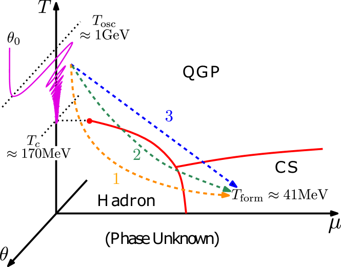
Figure 1: This diagram illustrates the interrelation between the axion production due to the misalignment mechanism and the nugget’s formation which starts before the axion field $\theta$ relaxes to zero. Adopted from Ge:2017idw .

In particular, it is known that the spectrum from galactic center (where the dark and visible matter densities assume the high values) contains several excesses of diffuse emission the origin of which is unknown, the best known example being the strong galactic 511 KeV line. If the nuggets have the average baryon number in the $\langle B\rangle\sim(10^{25}-10^{26})$ range they could offer a potential explanation for several of these diffuse components. It is important to emphasize that a comparison between emissions with drastically different frequencies in such computations is possible because the rate of annihilation events (between visible matter and antimatter DM nuggets) is proportional to one and the same product of the local visible and DM distributions at the annihilation site. The observed fluxes for different emissions thus depend through one and the same line-of-sight integral

$$\Phi\sim R^{2}\int d\Omega dl[n_{\rm visible}(l)\cdot n_{DM}(l)],$$ (4)

where $R\sim B^{1/3}$ is a typical size of the nugget which determines the effective cross section of interaction between DM and visible matter. As $n_{DM}\sim B^{-1}$ the effective interaction is strongly suppressed $\sim B^{-1/3}$. The parameter $\langle B\rangle\sim(10^{25}-10^{26})$ was fixed in this proposal by assuming that this mechanism saturates the observed 511 KeV line Oaknin:2004mn ; Zhitnitsky:2006tu , which resulted from annihilation of the electrons from visible matter and positrons from antinuggets. Other emissions from different frequency bands are expressed in terms of the same integral (4), and therefore, the relative intensities are unambiguously and completely determined by internal structure of the nuggets which is described by conventional nuclear physics and basic QED. In particular, this model offers a potential explanation for several of these diffuse components (including 511 KeV line and accompanied continuum of $\gamma$ rays in 100 KeV and few MeV ranges, as well as x-rays, and radio frequency bands). For further details see the original works Oaknin:2004mn ; Zhitnitsky:2006tu ; Forbes:2006ba ; Lawson:2007kp ; Forbes:2008uf ; Forbes:2009wg ; Lawson:2012zu with specific computations in different frequency bands in galactic radiation, and a short overview Lawson:2013bya .

Another domain where the coupling between AQN and visible matter could produce some observable effects is related to the recent EDGES (Experiment to Detect the Global Epoch of reionization Signatures) observation of a stronger than anticipated 21 cm absorption Bowman:2018yin . It has been argued in Lawson:2018qkc that this stronger than anticipated 21 cm absorption can find its natural explanation within the AQN framework. The basic idea is that the extra thermal emission from AQN dark matter at early times produces the required intensity (without adjusting any parameters) to explain the recent EDGES observation.

Yet another the AQN-related effect might be intimately linked to the so-called “solar corona heating mystery”. The renowned (since 1939) puzzle is that the corona has a temperature $T\simeq 10^{6}$K which is 100 times hotter than the surface temperature of the Sun, and conventional astrophysical sources fail to explain the extreme UV (EUV) and soft x ray radiation from the corona 2000 km above the photosphere. Our comment here is that this puzzle might find its natural resolution within the AQN framework as recently argued in Zhitnitsky:2017rop ; Raza:2018gpb .

To be more specific, if one estimates the extra energy being injected when the anti-nuggets annihilate with the solar material one obtains a total extra energy $\sim 10^{27}{\rm erg}/{\rm s}$ which automatically reproduces the observed EUV and soft x-ray energetics Zhitnitsky:2017rop . This estimate is derived exclusively in terms of known dark matter density $\rho_{\rm DM}\sim 0.3~{}{\rm GeVcm^{-3}}$ and dark matter velocity $v_{\rm DM}\sim 10^{-3}c$ surrounding the Sun without adjusting any parameters of the model. This estimate is strongly supported by Monte Carlo numerical computations Raza:2018gpb which suggest that most annihilation events occur precisely at the so-called transition region at an altitude of $2000$ km, where is known that drastic changes in temperature and density occur.

In the AQN framework the baryon number distribution must be in the range

$$10^{23}\leq|B|\leq 10^{28}$$ (5)

to be consistent with modelling on solar corona heating related to the energy injection events (the so-called “nanoflares”) with typical energies $E_{\rm nanoflares}\sim(m_{p}c^{2})B$. It is a highly nontrivial consistency check for the proposal Zhitnitsky:2017rop ; Raza:2018gpb that the required window (5) for nanoflares is consistent with the range of mean baryon number allowed by the axion and dark matter search constraints as these come from a number of different and independent constraints extracted from astrophysical, cosmological, satellite and ground based observations.

A “smoking gun” supporting the proposal Zhitnitsky:2017rop ; Raza:2018gpb on the nature of the EUV from corona would be the observation of the axions which will be radiated from the corona when the nuggets get disintegrated in the Sun. The corresponding computations have been carried out recently in Fischer:2018niu ; Liang:2018ecs . Presently the CAST (CERN Axion Search Telescope) Collaboration has taken a significant step to upgrade the instrument to make it sensitive to the spectral features of the axions produced due to the AQN annihilation events on the Sun.

Another inspiring observation indirectly supporting the AQN scenario can be explained as follows. It was recently claimed in ref. Zioutas that a number of highly unusual phenomena observed in the solar atmosphere can be explained by the gravitational lensing of “invisible” streaming matter towards the Sun. The phenomena include, but not limited to such irradiation as the EUV emission, frequency of X and M flare occurrences, etc. Naively, one should not expect any correlations between the flare occurrences, the intensity of the EUV radiation, and the position of the planets. Nevertheless, the analysis Zioutas obviously demonstrates that this naive expectation is not quite correct. At the same time, the emergence of such correlations within AQN framework is a quite natural effect. This is because the dark matter AQNs can play the role of the “invisible” matter in ref. Zioutas , which triggers otherwise unexpected solar activity sparking also the large flares Zhitnitsky:2018mav . Therefore, the observation of the correlation between the EUV intensity and frequency of the flares can be considered as an additional supporting argument of the AQN related dark matter explanation of the observed EUV irradiation because both effects are originated from the same dark matter AQNs.

We conclude this overview section on the AQN model with the following comment. The AQN framework is consistent with all known astrophysical, cosmological, satellite and ground based constraints. Furthermore, in a number of cases (when an enhancement factors have emerged) some observables become very close to present day constraints. In fact, in some cases the predictions of the model may explain a number of the long standing mysteries as highlighted above.

The goal of the present work is to argue that there is one more such case when some enhancements (during the BBN times) may lead to the consequences which are observed today. To be specific, the claim of the present work is that the the nuclei with $Z\geq 3$ during (or soon after BBN times) are prone to be trapped by negatively charged antinuggets at $T\simeq 20$ KeV. Some portion of these $Z\geq 3$ nuclei will be eventually annihilated inside the cores of the antinuggets. The probability for this process to occur will be proportional to the enhancement factor $\sim\exp(Z)$ which, as we argue below, will overcome a generic feature that the nuggets play no role in BBN physics as stated in item 3 above. If further analysis and studies confirm this claim it would represent a long-awaited resolution of the Primordial Lithium Puzzle within AQN framework.

III The internal structure of the nuggets

In this section we overview some essential technical details related to the internal structure of the AQN. We start in subsection III.1 with overview of key points from Lawson:2018qkc with analysis of the AQNs at high temperature $T>2m_{e}$ when large number of positrons are present in the system. In Subsection III.2 we overview few important results from Forbes:2009wg on structure of electro-sphere at low temperature $T\sim$eV. These results will play an important role in our main section IV where we present a precise mechanism which is capable to suppress the production of nuclei with $Z\geq 3$, which represents the main goal of our studies.

III.1 Pre-BBN cosmology: AQN annihilation events and energy injection

We follow Lawson:2018qkc to highlight few estimates related to the AQN evolution during the pre-BBN cosmology with $T>2m_{e}\sim 1$ MeV when the number densities of electrons, positrons, baryons and photons can be estimated as follows

$$n_{B} \sim n_{\gamma}\eta,~{}~{}\eta\sim 5\cdot 10^{-10},~{}~{}n_{\gamma}\sim\frac{2}{\pi^{2}}T^{3},$$ (6)

$$n_{e} \sim n_{e^{+}}\sim n_{\gamma},~{}~{}~{}n_{B}\sim 10^{22}{\rm cm^{-3}}\left(\frac{T}{1~{}MeV}\right)^{3}.$$

as the thermodynamical equilibrium is maintained in surrounding plasma. As we highlight below, the presence of the AQNs does not modify the thermodynamics of the plasma at high temperature and relations (6) basically stay the same. In particular, the rate of energy injection is negligible in comparison with average plasma energy density. Therefore, the presence of the nuggets does not modify the standard pre-BBN cosmology.

The basic reason for this conclusion as mentioned in item ${\bf 1}$ from previous section is that the number density of the nuggets $n_{\rm AQN}\sim B^{-1}$ is very tiny due to the very large baryon charge of a nugget, $B>10^{23}$. A small energy injection rate to be estimated below is the direct manifestation of this suppression factor.

The number of $e^{+}e^{-}$ annihilation events per unit time between electrons from plasma and positrons from nugget’s electrosphere for a single nugget can be estimated as follows

$$\frac{dN}{dt}\sim 4\pi R^{2}n_{\rm e}c$$ (7)

where $n_{e}$ is number density of electrons from plasma, and we assume that electrons hitting the nugget of size $R$ will get annihilated as the density of the positron in electrosphere is large as we discuss in next subsection III.2. The energy injection per unit time for a single nugget can be estimated from (7) by multiplying a typical energy $\sim\mu_{e^{+}}$ being produced as a result of annihilation:

$$\mu_{e^{+}}\frac{dN}{dt}\sim 4\pi R^{2}n_{\rm e}c\mu_{e^{+}},.$$ (8)

where $\mu_{e^{+}}$ is the chemical potential of the positrons from nugget’s electrosphere, see next subsection. The energy injection per unit volume per unit time can be estimated as

$$\frac{dE}{dVdt}\sim 4\pi R^{2}n_{\rm AQN}n_{\rm e}c\mu_{e^{+}},$$ (9)

where the AQN number density $n_{\rm AQN}$ from (9) is estimated as follows

$$n_{\rm AQN}\sim\frac{n_{B}}{\langle B\rangle}\sim\eta\frac{n_{\gamma}}{\langle B\rangle}\sim\frac{T^{3}\eta}{\langle B\rangle}\sim 5\cdot 10^{-36}T^{3},$$ (10)

where $\eta$ is conventional the baryon to photon ratio factor (6). For numerical estimates we used $\langle B\rangle\simeq 10^{26}$. We want to estimate the total amount of energy being injected into the system per unit volume during mean free time $\tau\sim(\alpha^{2}T)^{-1}$ which is defined as a typical time between collisions. During time $\tau$ the system adjusts any injection of the external energy into the system due to the fast equilibration. We want to compare this extra injected energy (as a result of annihilation events of electrons with positrons from electrosphere) with typical energy density in the system $\sim(Tn_{\rm e})$, i.e. we consider the dimensionless ratio

$$\frac{\tau}{Tn_{\rm e}}\cdot\left(\frac{dE}{dVdt}\right)\sim\frac{\left(\eta R^{2}T\mu_{e^{+}}\right)}{\alpha^{2}\langle B\rangle}\sim 10^{-18}\left(\frac{T}{1~{}\rm MeV}\right),~{}~{}~{}~{}$$ (11)

where we use $\mu_{e^{+}}\sim 10$ MeV for numerical estimates, see next subsection.

It is clear that such small amount of energy injected into the system will be quickly equilibrated within the system such the standard pre-BBN cosmology remains intact. In other words, the conventional equation of state, and conventional evolution of the system is unaffected by presence of AQNs at $T>2m_{e}$ when the positrons in plasma are in thermal equilibrium and easily available to replace the positrons from antinugget’s electrosphere. The basic reason for this conclusion is due to the fact that the number density of the AQNs is very tiny according to (10) such that the conventional interaction of the AQNs with surrounding material in normal circumstances is strongly suppressed due to $\langle B\rangle^{-1}$ factor.

III.2 Electrosphere Structure

We need one more ingredient for our future analysis in Sect. IV suggesting that in some circumstances the AQNs can drastically modify the conventional BBN outcome. This additional ingredient is related to analysis of electrosphere of the AQN at $T\ll m_{e}$ when it is placed into a dilute system (such as Inter-Stellar Medium (ism)) where very few particles are present in the system. The corresponding studies have been carried out in Forbes:2009wg and played an important role in analysis of access of radiation from the galactic center as reviewed in previous section, see few paragraphs around eq.(4). We overview the basic ideas of computations Forbes:2009wg in this subsection to make our presentation self-contained.

The basic idea of Forbes:2009wg is to use Thomas-Fermi analysis including the full relativistic electron equation of state required to model the relativistic regime close to the nuclear core. One should emphasize that the presence of electrosphere itself is a very generic phenomenon, and its main features are determined by the boundary conditions deep inside the nugget (being in CS phase) where the lepton’s chemical potential is fixed as a result of the beta equilibrium, similar to analysis of refs Alcock:1986hz ; Kettner:1994zs in the context of strange stars.

The density profile of the electrosphere has been derived in Forbes:2009wg from a density functional theory after neglecting the exchange contribution, which is suppressed by the weak coupling $\alpha$. The electrostatic potential $\phi(r)$ must satisfy the Poisson equation

$$\nabla^{2}\phi(r)=-4\pi en(r).$$ (12)

where $en(r)$ is the charge density which can be expressed in terms of the chemical potential

$$\mu(r)=\mu-e\phi(r).$$ (13)

The resulting equation assumes the form

$$\nabla^{2}\mu(r)=4\pi\alpha n[\mu(r)],~{}~{}~{}\epsilon_{p}=\sqrt{p^{2}+m^{2}}$$ (14)

$$n[\mu]=2\!\int\!\!\frac{{\rm d}^{3}{p}}{(2\pi)^{3}}\!\left[\frac{1}{1+e^{(\epsilon_{p}-\mu)/T}}-\frac{1}{1+e^{(\epsilon_{p}+\mu)/T}}\right],$$

In (14) both particle and antiparticle contributions have been explicitly included, and $e^{2}=\alpha$ in units where $\hbar=c=4\pi\epsilon_{0}=1$.

Few comments on the boundary conditions which have been imposed in analysis Forbes:2009wg . The boundary conditions at $r=R$ (at the nugget’ surface) are determined by the beta equilibrium, similar to analysis in the context of strange stars Alcock:1986hz ; Kettner:1994zs . In context of CS dense matter a similar condition applies. However, a precise structure in CS phase is not known, and therefore, $\mu(R)$ at the boundary $R$ which depends on equation of state for the quark-matter phase is also not known. Typical QCD based estimates suggest that lepton chemical potential $\mu$ is of order $\approx 25$ MeV, see e.g. review Alford:2007xm . This is the value which was adopted in Forbes:2009wg for numerical estimates.

Another parameter from studies Forbes:2009wg is the outer radius $r_{*}$ of electrosphere where nuggets will “radiate” the loosely bound positrons until the electrostatic potential is comparable to the temperature $\alpha Q/r_{*}\sim T$, where $eQ$ is the charge of the AQNs due to the ionization at temperature $T$.

The equation (14) with the corresponding boundary conditions as explained above has been solved numerically   Forbes:2009wg with the profile function which smoothly interpolates from ultra-relativistic regime deep inside the nugget and one for the non-relativistic Boltzmann regime  Forbes:2009wg where $n[\mu]\propto e^{\mu/T}$ at $z\equiv(r-R)$ far away from the nugget’s surface which is defined as $z=0$.

For non-relativistic Boltzmann regime one can approximately describe the density of positrons in electrosphere as follows Forbes:2008uf :

$$n_{e^{+}}(z)=\frac{T}{2\pi\alpha}\frac{1}{(z+\bar{z})^{2}},~{}~{}~{}~{}\frac{1}{\bar{z}}=m_{e}\sqrt{2\pi\alpha}\left(\frac{T}{m_{e}}\right)^{1/4}$$ (15)

where $\bar{z}$ is the integration constant is chosen to match the Boltzmann regime at sufficiently large $z\gg\bar{z}$. Numerical studies   Forbes:2009wg support the approximate analytical expression (15).

The same expression (15) for the positron density in electrosphere as the solution of the Thomas-Fermi equations can be also represented in terms of the chemical potential as these two parameters are related according to eqs.(13) and (14), see Forbes:2008uf with details,

$$n_{e^{+}}[\tilde{\mu}]=\sqrt{2}\left(\frac{mT}{\pi}\right)^{3/2}e^{\tilde{\mu}/T},~{}~{}~{}~{}\tilde{\mu}\equiv\mu(r)-m_{e},$$ (16)

where we redefined the chemical potential by removing a large constant term $m_{e}$ to make it appropriate for non-relativistic regime.

We conclude this overview section on electrosphere’s structure with the following comments. The results presented above are well suited for studies of the AQNs in low temperature and low density environment such as Inter-Stellar Medium in our galaxy. The goal of the present work is drastically different as it deals with relatively high temperature plasma with $T\sim 20$ KeV soon after the BBN epoch. Why the temperature $T\sim 20$ KeV is so special for our analysis? This is because at $T\approx 20$ KeV the positron number density in plasma assumes the same order of magnitude as the baryon number density $n_{B}\simeq\eta n_{\gamma}$. When the temperature becomes slightly lower, i.e. $T<20$ KeV, the positrons will be soon completely annihilated while the proton number density essentially remains the same as $n_{B}=\eta n_{\gamma}$. In context of our work it implies that the screening of the negative charge of the antinugget will be provided by the protons at $T<20$ KeV as explained in next section.

IV The AQN-induced suppression mechanism for large $Z\geq 3$

IV.1 Preliminaries

The starting point for our analysis is the observation that the high temperature environment leads to ionization of the loosely bound positrons such that the antinuggets will become negative charged ions with charge $-Q$ estimated as follows

$$Q\simeq 4\pi R^{2}\int^{\infty}_{z_{0}}n(z)dz\sim\frac{4\pi R^{2}}{2\pi\alpha}\cdot\left(T\sqrt{2m_{e}T}\right)~{}~{}~{}~{}~{}$$ (17)

where we assume that the positrons with $p^{2}/(2m_{e})<T$ will be stripped off the electrosphere as a result of high temperature $T$. These loosely bound positrons are localized mostly at outer regions of electrosphere at distances $z>z_{0}=(2m_{e}T)^{-1/2}$ which motivates our cutoff in estimate (17). For these estimates we also used an approximation (15) from Section III.2 to express $Q$ in a simple analytical form (17).

One should emphasize that the mean-field approximation is not justified at very large distances. Furthermore, an approximate analytical expression (15) used in estimate (17) is sufficiently good approximation for distances close to the surface when one-dimensional treatment in terms of $z\ll R$ is appropriate, but breaks down for distances $z\gg R$ when effectively 3D treatment is required. However, these deficiencies do not drastically modify our estimate (17) for the total charge $Q$ as the dominant contribution to the integral (17) comes from small $z\ll R$ where the approximate solution (15) is valid.

The key observation of the present work is that the positrons which are stripped off due to the high temperature will be replaced by the positively charged protons. This process inevitably should take place to neutralize the large negative charge $Q$ estimated by eq (17). Before we proceed with corresponding estimates it is very instructive to compare the charge density of the protons which will be accumulated in vicinity of the nugget’s surface with average proton’s density (6) far away from the nuggets in plasma.

The proton’s charge density will have essentially the same qualitative behaviour as (15) similar to the positron’s charge density (if the positrons were not stripped off) representing the solution of the Thomas -Fermi equation. The only difference is that for proton’s density profile $n_{p}(z)$ we fix the integration constant $\bar{z}_{p}$ assuming that the protons neutralize the negative charge $Q$ given by (17). This boundary conditions should be contrasted with our studies in Section III.2 for positrons where boundary conditions were imposed by matching the chemical potential generated due to the $\beta$ equilibrium deep inside the nuggets.

Therefore, the estimation for the proton density in close vicinity of the surface $n_{p}(z)$ is very similar to estimates (15) when the Thomas -Fermi approximation can be trusted, i.e.

$$n_{p}(z)=\frac{T}{2\pi\alpha}\frac{1}{(z+\bar{z}_{p})^{2}},~{}~{}~{}z\ll R$$ (18)

where the integration constant $\bar{z}_{p}$ is fixed by the condition

$$\int_{0}^{\infty}n_{p}(z)dz=Q=\frac{4\pi R^{2}T}{2\pi\alpha}\frac{1}{\bar{z_{p}}},~{}~{}~{}\frac{1}{\bar{z_{p}}}=\sqrt{2m_{e}T}.~{}~{}~{}$$ (19)

The density of protons at $z=0$ is huge

$$n_{p}(z=0)=\frac{T}{2\pi\alpha}\frac{1}{\bar{z_{p}}^{2}}\simeq 1.3\cdot 10^{30}{\rm cm^{-3}}\left(\frac{T}{20~{}{\rm KeV}}\right)^{2}.~{}~{}~{}$$ (20)

One should emphasize that the total accumulated charge $Q$ due to the screening by protons (19) is the surface effect. Therefore, baryon charge in form of the protons (19) represents a very small fraction of the total baryon charge hidden in the nuggets, i.e. $Q/B\ll 1$. The direct annihilation of the protons surrounding the anti-nugget is strongly suppressed due to the large gap in CS phase as mentioned in item 3 in Section II.

It is instructive to compare (20) with the protons’ density $n_{B}$ outside the nugget in plasma given in (6). The ratio of the densities $n_{B}$ and $n_{p}(z=0)$ is estimated as

$$\left[\frac{n_{B}(T)}{n_{p}(z=0,T)}\right]\sim 6\cdot 10^{-14}\left(\frac{T}{20~{}{\rm KeV}}\right).$$ (21)

It depends on $T$ because $n_{B}\sim T^{3}$ has conventional scaling while $n_{p}(z=0)\sim T^{2}$ is the surface effect, and does not follow the free particle distribution.

We need yet another ingredient for presenting the suppression mechanism for heavy nuclei with $Z\geq 3$. We define the capture radius $R_{\rm cap}(T)$ as the distance when the external protons from plasma have sufficiently low velocities such that they can be captured (trapped) by long ranged Coulomb forces and become bounded to the antinugget, i.e.

$$\frac{\alpha Q(r)}{r}>\frac{m_{p}v^{2}}{2}\approx T~{}~{}~{}{\rm for}~{}~{}~{}r\leq R_{\rm cap}(T).$$ (22)

We estimate $R_{\rm cap}(T)$ (which is obviously much larger than the size of the nugget $R_{\rm cap}(T)\gg R$) and related parameters in next section IV.3. It is expected that at $r\geq R_{\rm cap}$ the density of the protons in electrosphere becomes the same order of magnitude as the average density of the plasma $n_{B}$ which itself is determined exclusively by the temperature according to (6).

Final comment we would like to make in this subsection is that the ratio $\xi$ defined as

$$\xi(r,T)\equiv\frac{\alpha Q(r)}{rT}$$ (23)

will play very important role in our arguments which follow. The parameter $\xi(r,T)$ obviously describes the ratio of the potential binding energy in comparison with kinetic energy $\sim T$. Important parameter to be discussed below is the average characteristic $\langle\xi(T)\rangle$ which represents the mean value of this ratio over entire ensemble of the particles surrounding the antinugget.

IV.2 Few relevant estimates

We start our analysis with numerical estimate the capture radius $R_{\rm cap}(T)$ as defined by (22). We assume that the density $n_{p}(r=R,T)$ has a power like behaviour at $r\gtrsim R$ with exponent $p$. This assumption is consistent with our numerical studies Forbes:2009wg of the electrosphere with $p\simeq 6$. It is also consistent with conventional Thomas-Fermi model at $T=0$, see e.g. Landau textbook Landau . We keep parameter $p$ to be arbitrary to demonstrate that our main claim is not very sensitive to our assumption on numerical value of $p$.

Therefore, we parameterize the density as follows

$$n_{p}(r,T)\simeq n_{p}(r=R,T)\left(\frac{R}{r}\right)^{p},~{}~{}~{}$$ (24)

where $n_{p}(r=R)\equiv n_{p}(z=0)$ is the surface density determined by the eq. (20). We can now estimate the effective capture distance $R_{\rm cap}$. It can be approximately computed from the following condition

$$n_{p}(R_{\rm cap},T)\simeq n_{p}(z=0,T)\left(\frac{R}{R_{\rm cap}}\right)^{p}\simeq n_{B}(T)$$ (25)

where $n_{B}(T)$ defined by (6) is the average proton number density far away from the nuggets. From (25) and (21) we estimate effective capture distance $R_{\rm cap}$ as follows

$$\left(\frac{R}{R_{\rm cap}}\right)^{p} \simeq 6\cdot 10^{-14}\left(\frac{T}{20~{}\rm KeV}\right)$$ (26)

In particular for $p\simeq 6$ the effective capture distance $R_{\rm cap}$ is of order

$$R_{\rm cap}\simeq 1.6\cdot 10^{2}\cdot\left(\frac{20~{}\rm KeV}{T}\right)^{\frac{1}{p}}R\simeq 3\cdot 10^{-3}{\rm cm}$$ (27)

for typical size of the nugget $R\simeq 2\cdot 10^{-5}{\rm cm}$ and $p=6$.

Our next task is to estimate the screened charge $Q(r\sim R_{\rm cap})$ at large distances $r\sim R_{\rm cap}$ far away from the nugget’s core. We assume that this is the region where the power like behaviour (24) for the density $n_{p}(r)$ still holds, and the expected exponential tail (which cannot be accommodated within a simple mean-field approximation adopted in this work) is not yet operational. This screened charge is obviously must be much smaller that the original charge (19). Indeed, within our framework one can compute the screened charge by integrating from $R_{\rm cap}$ to infinity instead of accounting for the cancellations between the original negative charge of the antinugget and positive charge of the surrounding protons, i.e.

$$Q(R_{\rm cap})\simeq\int_{R_{\rm cap}}^{\infty}4\pi r^{2}drn_{p}(r)\sim\frac{4\pi n_{B}(T)R^{3}_{\rm cap}(T)}{(p-3)},~{}~{}~{}~{}~{}$$ (28)

where $n_{p}(r)$ is the charge density determined by (24), and we expressed the final formula in terms of the background baryon density $n_{B}(T)$ at temperature $T$. It is known that at much larger distances the behaviour must be changed to $\exp(-r)$ due the screening at very large distance $r$, but the integral (28) is saturated by much smaller $r\sim R_{\rm cap}$; therefore we ignore the small corrections due to the exponential tail. It is useful for what follows to represent formula (28) in the form which explicitly shows the $T$ dependence and the algebraic exponent $p$:

$$Q(R_{\rm cap})\sim 10^{10}\cdot\left(\frac{T}{20~{}\rm KeV}\right)^{3(1-\frac{1}{p})},$$ (29)

where for the numerical estimates we use $R\simeq 2\cdot 10^{-5}{\rm cm}$.

It is also instructive to estimate the number of particles being affected by the presence of the AQNs in the system. To estimate this ratio of the “affected particles” one should multiply (29) by the density of the antinuggets (10) and compare the obtained result with the average baryon density $n_{B}(T)$ in plasma, i.e.

$$\frac{\delta n_{p}}{n_{p}}\sim\frac{\left[n_{\rm AQN}\cdot Q(R_{\rm cap})\right]}{n_{B}}\sim 3\cdot 10^{-16}\left(\frac{T}{20~{}\rm KeV}\right)^{3(1-\frac{1}{p})}.~{}~{}~{}~{}$$ (30)

The density of the antinuggets $n_{\rm AQN}$ in this formula is estimated as

$$n_{\rm AQN}\simeq\frac{n_{B}}{\langle B\rangle}\cdot 5\cdot\frac{3}{5},$$ (31)

where factor $3/5$ accounts for the portion of the antinuggets, while factor $5$ accounts for approximate ratio $\rho_{\rm DM}\simeq 5\rho_{\rm B}$ when it is assumed that the DM is saturated by nuggets and antinuggets.

The number of affected particles ${\delta n_{p}}/{n_{p}}$ as one can see from estimate (30) is absolutely negligible, as expected. This claim is similar to analogous estimates in pre-BBN cosmology expressed by formula (11). In both cases the strong suppression is a result of very tiny number density of the AQNs such that the conventional interaction of the AQNs with surrounding material in normal circumstances is strongly suppressed by factor $\langle B\rangle^{-1}$ in comparison with visible baryon interactions.

IV.3 Suppression Mechanism for heavy nuclei

We are in position now to formulate the basic idea for the suppression mechanism for heavy nuclei which goes as follows. In previous sections in our analysis related to the screening of the original antinugget’s charge we had assumed that all the particles which screen the negative electric charge $-eQ$ are the protons which have positive unit electric charge $+e$. The corresponding density $n_{p}$ in the vicinity of the nugget’s core is determined by eq. (18), and represents the self-consistent solution in mean-field approximation. The presence of heavier nuclei with $Z>1$ do not qualitatively change the structure of the electrosphere as long as densities of these nuclei $n_{Z}$ are sufficiently small in comparison with the background proton density $n_{B}$, i.e. $n_{Z}\ll n_{B}$.

However, the interaction of these heavy nuclei with the nugget’s charge $Q$ is exponentially stronger due to the Boltzmann enhancement. It can be seen explicitly from formula (16) represented in terms of the chemical potential which itself is expressed in terms of electrostatic potential (13). We would like to represent the corresponding enhancement factor in the following way

$$\sim\exp\left[{\frac{(Z-1)\alpha Q(r)}{rT}}\right]$$ (32)

where we inserted an additional factor $(Z-1)$ into the expression to avoid the double counting. Indeed, the protons with $Z=1$ have been accounted for in the Thomas-Fermi computations leading to (16). Precisely this Boltzmann (Fermi for degenerate case) distribution leads to high density of protons close to the nugget’s surface (20).

Now we are in position to compute the relative number of the trapped and captured ions with $Z>1$. The corresponding estimate goes exactly in the same way as our estimates with protons (30) with $Q(R_{\rm cap})$ given by (28)

$$\frac{\delta n_{Z}}{n_{Z}}\simeq\frac{4\pi R^{3}_{\rm cap}}{3}\cdot n_{AQN}\cdot\exp\left[{\frac{(Z-1)\alpha Q(r)}{rT}}\right],$$ (33)

where we inserted the enhancement factor (32) as explained above. We want to avoid the double counting of the particles with charges $Z=1$. Therefore, we introduce the factor $(Z-1)$ in (33) and treat it as an enhancement factor for ions (He, Li and Be) in comparison with protons. Note that the density $n_{Z}$ is very small in comparison with the density of protons and does not perturb their distribution. In the relative estimate in eq. (33) it enters the numerator and denominator and cancels out while enhancement factor (32) obviously stays.

It is convenient to estimate the dimensionless suppression factor (first two factors from eq. (33)) as follows

$$\left[\frac{4\pi R_{\rm cap}^{3}}{3}\cdot n_{AQN}\right]\sim 2.7\cdot 10^{-16}\left(\frac{T}{20~{}\rm KeV}\right)^{3(1-\frac{1}{p})},~{}~{}~{}~{}$$ (34)

We want to rewrite this dimensionless factor in the exponential form as all elements are highly (exponentially) sensitive to many unknown parameters, i.e.

$$\left[\frac{4\pi R^{3}_{\rm cap}}{3}\cdot n_{AQN}\right]\simeq\exp(-X_{\rm Sup}),~{}~{}~{}$$

$$X_{\rm Supp}\simeq 35.8-3\left(1-\frac{1}{p}\right)\ln\left(\frac{T}{\rm 20~{}KeV}\right).$$ (35)

Now we want to argue that the last dimensionless factor $\sim\exp(...)$ in eq. (33) represents a huge enhancement for ions such as Li with $Z=3$ and Be with $Z=4$, while it remains to be relatively small for He with $Z=2$ and vanishes for H with $Z=1$. We proceed with estimates of the enhancement factor entering (33) by assuming that the screened charge of the antinugget $Q(R_{\rm cap})$ is estimated at $r\simeq R_{\rm cap}$ as given by in eqs. (28) and (29):

$$\left({\frac{\alpha Q(R_{\rm cap})}{R_{\rm cap}T}}\right)\sim 20\cdot\left(\frac{T}{20~{}\rm KeV}\right)^{2(1-\frac{1}{p})}.$$ (36)

We want represent the enhancement factor entering (36) in the same exponential way as the suppression factor (IV.3), i.e.

$$\exp\left[(Z-1)\cdot{\frac{\alpha Q(R_{\rm cap})}{R_{\rm cap}T}}\right]=\exp(+X_{\rm Enh}),$$

$$~{}~{}~{}X_{\rm Enh}\simeq 20(Z-1)\cdot\left(\frac{T}{20~{}\rm KeV}\right)^{2(1-\frac{1}{p})}.$$ (37)

The relative number of the trapped and captured ions defined by (33) is estimated now as follows

$$\frac{\delta n_{Z}}{n_{Z}}\simeq e^{(-X_{\rm Supp}+X_{\rm Enh})}$$ (38)

where $X_{\rm Supp}$ and $X_{\rm Enh}$ are estimated by eqs. (IV.3) and (IV.3) correspondingly. For our purposes of order of magnitude estimate one can neglect the $\ln$ term in (IV.3) and $1/p$ in (IV.3) to approximate the final formula for the exponent for $Z=3$ as follows

$$\left(-X_{\rm Supp}+X_{\rm Enh}\right)\simeq\left[-36+40\cdot\left(\frac{T}{20~{}\rm KeV}\right)^{2}\right],$$ (39)

which suggests that relative number of the remaining Li ions might be strongly depleted as ${\delta n({Li}})/{n({Li})}\sim 1$ because the depletion becomes order of one effect for $T\approx 20$ KeV. For Be ions the depletion effect is even stronger. The depletion effect for He with $Z=2$ can be ignored as the enhancement factor (IV.3) is insufficient to overcome the suppression factor (IV.3) in this case. One should also remark here that we do not discriminate ⁶Li and ⁷Li in our estimates. In fact in our effective mean field approximation it would be very hard to do so, especially due to the fact that ⁶Li density is strongly suppressed in comparison with ⁷Li. Therefore, the only claim one can make is that the ions with charges $Z=3$ are strongly depleted as eq. (39) states.

In our estimates (38), (39) we, of course, assume that the finite portion of the Li ions will be affected by the nuggets during the cosmic time $t_{0}\sim 2\cdot 10^{3}$s corresponding to the temperature $T\approx 20$ keV. We refer to Appendix A where we estimate the fluxes of the ions entering the AQNs vicinity of size $R_{\rm cap}$. We argue in Appendix A that a finite portion of all ions in entire volume will be affected by the nuggets. However, the eventual effect of this impact of the nuggets is negligible for light nuclei with $Z\leq 2$ and becomes crucial for heavy ions with $Z\geq 3$ as our estimates (38), (39) suggest.

Formula (39) is indeed an amazing result which might be the resolution of the primordial Li problem as finite portion of the produced Li gets captured by the antinuggets at $T\simeq 20~{}{\rm KeV}$ soon after the BBN ended. It is important to emphasize that no any special fitting procedures have been employed in the estimates presented above. All parameters which have been used to arrive to the final expression (38), (39) assume the same values similar to our previous studies related to the galactic excess emission, estimates related to EDGES observations, and resolution of the solar corona heating puzzle within AQN model as reviewed in Sect. II.

Few comments are in order. First of all, our assumption on specific algebraic exponent $p\simeq 6$ is not crucial as the final results are not very sensitive to this assumption. Our estimates are obviously very sensitive to the parameters of the nuggets, such as typical baryon charge $B$, radius of the nugget, $R$, etc. One should emphasize that all these typical parameters are consistent with cosmological, astrophysical and ground based constraints as overviewed in Section II. Furthermore, these parameters are consistent with axion search experiments constraints as parameters $R$ and $m_{a}$ are not independent, but related to each other.

V Conclusion and future directions

The main result of the present work is represented by equations (38) and (39) which show that the primordial abundance of ⁷Li nuclei could be much smaller than conventional computations ParticleData predict. The effect is due to the capture and subsequent annihilation of Li and Be ions by antinuggets within AQN paradigm.

A proper procedure would be, of course, integrating over time evolution and averaging over the nugget’s size distribution, similar to studies Raza:2018gpb on the solar nanoflare distribution as overviewed in Section II. It was not the goal of the present work to carry out precise computations of the effect. Such a study would not be sufficiently precise procedure anyway because of a huge (exponential) sensitivity to the parameters $R,B$ and their distributions which are not well known. Rather, our intention was to demonstrate that the resolution of the primordial Li puzzle might be a very natural outcome of presence of the AQNs in the plasma, and their interactions with the visible matter soon after BBN formation epoch.

One should emphasize that the estimate (38), (39) formally makes sense as long as $({\delta n_{Z}}/{n_{Z}})\ll 1$. However, the point is that $({\delta n_{Z}}/{n_{Z}})$ could easily assume a value of order one. It unambiguously implies that a finite portion of Li and Be nuclei from plasma get trapped by the antinugget’s electrosphere.

We believe that our order of magnitude estimates (38), (39) represent sufficiently convincing arguments supporting the claim that $({\delta n_{Z}}/{n_{Z}})\sim 1$ for Li with $Z=3$ and Be with $Z=4$. Indeed, we demonstrated that the internal properties of the nuggets are such that the heavy nuclei with $Z\geq 3$ are strongly attracted to the antinuggets due to the long range Coulomb forces. These heavy nuclei will be bounded to the antinuggets and will eventually get annihilated in the AQN’s cores in subsequent time evolution .

One should emphasize that the corresponding key parameters of the nuggets which have been used in our estimates have not been specifically chosen for the purposes of the present work devoted to the resolution of the primordial Li puzzle (as it is normally done in a typical proposal on resolving Li puzzle within WIMP framework). Instead, all the key parameters have been originally fixed for very different purposes to satisfy a variety of constraints from a number of unrelated experiments and observations as reviewed in Sect. II.

Therefore, the resolution of the Li puzzle within AQN framework represents yet another indirect support for this new paradigm on the nature of DM and baryon charge separation replacing the conventional “baryogenesis”. The list of these indirect evidences supporting the AQN framework includes (but not limited) such long standing problems as a natural explanation of the observed ratio $\Omega_{\rm dark}\sim\Omega_{\rm visible}$, renowned puzzle coined as the “solar corona heating mystery”, recent EDGES observations, to name just a few, see overview in Sect. II.

To reiterate: this AQN model was invented to explain the observed ratio (2) in a natural way as both types of matter (visible and dark) are formed during the same QCD epoch in early Universe, and proportional to one and the same dimensional parameter $\Lambda_{\rm QCD}$. Precisely the same generic feature plays a key role in the suppression mechanism for the abundance of heavy nuclei with $Z>2$ as presented in Sect. IV.3 because the visible nuclei and antinuggets made from the same Standard Model quarks and gluons (but in different phases, the hadronic phase and CS phase correspondingly).

Can we study any traces of the captured (after BBN epoch) heavy nuclei by antinuggets today? It is very unlikely as the captured heavy nuclei will eventually get annihilated in the antinugget’s core. Furthermore, it is hard to expect any specific electromagnetic signatures as a result of these annihilation processes of the heavy nuclei, see also footnote 6 with related comments.

In some circumstances, though, the antinuggets can be completely disintegrated, for example in the solar corona leading to the extreme UV radiation as reviewed in Sect. II. When the AQNs propagate in the earth’s atmosphere they obviously produce some observable effects. In fact, the propagating of the AQN in earth’s atmosphere can mimic the ultra high energy cosmic ray air showers as argued in Lawson:2010uz ; Lawson:2012vk ; Lawson:2013bya .

When the AQNs travelling in deep earth’s underground it is very unlikely to observe any specific $E\&M$ signatures from deep underground due to the annihilation processes. It is much more likely that the direct observations of the axions which will be inevitably released in the annihilation processes can be directly observed as recently suggested in refs Fischer:2018niu ; Liang:2018ecs . In fact, the observation of these axions with very distinct spectral properties in comparison with conventional galactic axions will be the smoking gun supporting the entire AQN framework, including the proposal on the primordial Li puzzle resolution as advocated in this work. We finish this work on this positive and optimistic note.

Appendix A Primordial nuclei fluxes in vicinities of the nuggets

The main goal of this Appendix is to argue that the flux of the ions hitting the AQNs surface is sufficiently large such that a finite portion of all ions from the system will enter the vicinity of the nuggets during cosmic time $t_{0}\sim 2\cdot 10^{3}$s. This is precisely the assumption as formulated in the text after eq. (39), and which is justified a posteriori.

We start with estimation of a number of ions with charge $Z$ entering the vicinity of a single antinugget per unit time

$$\frac{dN_{Z}}{dt}\sim 4\pi R_{\rm cap}^{2}n_{Z}v_{Z}$$ (40)

where capture size $R_{\rm cap}$ is defined by eqs.(25) and (26) and $v_{Z}$ is the ion’s velocity in the plasma. This expression represents a strong underestimation as it does not account for a huge remaining charge $Q(R_{\rm cap})$ at distance $R_{\rm cap}$ from the nugget. We will correct for this effect at the end of this Appendix.

We call the corresponding ions as “affected” by the presence of AQNs. The number density of the affected ions per unit volume $dV$ per unit time $dt$ can be estimated by multiplying (40) to the density of the antinuggets given by (31), i.e.

$$\frac{dN_{Z}}{dtdV}\sim n_{\rm AQN}\cdot\frac{dN_{Z}}{dt}\sim 4\pi R_{\rm cap}^{2}n_{\rm AQN}n_{Z}v_{Z}.$$ (41)

We are interested in a relative ratio of the affected ions, rather than in their absolute values. The corresponding ratio is estimated as follows,

$$\frac{1}{n_{Z}}\left(\frac{dN_{Z}}{dtdV}\right)\sim n_{\rm AQN}\cdot\frac{1}{n_{Z}}\frac{dN_{Z}}{dt}\sim 4\pi R_{\rm cap}^{2}n_{\rm AQN}v_{Z}.~{}~{}~{}~{}~{}$$ (42)

Now we want to estimate the total portion of affected ions by integrating over $\int dt$. To simplify the estimates we simply multiply (42) by time $t_{0}\sim 2\cdot 10^{3}$s corresponding to $T\approx 20$ keV because the integral is saturated by the highest possible temperature. The corresponding estimate reads

$$\int\frac{dt}{n_{Z}}\left(\frac{dN_{Z}}{dtdV}\right)\sim 4\pi R_{\rm cap}^{2}n_{\rm AQN}v_{Z}t_{0}\sim 0.1,$$ (43)

where for numerical estimates we used parameters for $R_{\rm cap}$ and $n_{\rm AQN}$ defined in the text. The estimate (43) implies that at least $10\%$ of all ions from plasma will be affected by the AQNs during the cosmic time $t_{0}$.

However, as already mentioned, the result (43) should be considered as a strong underestimation of the relevant portion of the affected ions because there is a systematic effect (yet, not accounted for) due to the presence of a gradient of the residual electric field in the direction to the antinugget as a result of uncompensated charge $Q(R_{\rm cap})$ at distance $R_{\rm cap}$ from the nugget as estimated by (29).

To account for the corresponding effect (which obviously enhances the ratio (43)) we assume that the residual charge $Q(R_{\rm cap})$ will be screened on distance $R_{\rm screen}$ determined by the condition

$$Q(R_{\rm cap})e^{-\frac{(R_{\rm screen}-R_{\rm cap})}{\lambda_{D}}}\sim 1,~{}~{}~{}~{}~{}\lambda^{2}_{D}\simeq\frac{T}{4\pi n_{p}\alpha}.$$ (44)

If one uses the numerical parameters for $T,R_{\rm cap}$, and $n_{p}$ from the text one arrives to the following estimate for $R_{\rm screen}$ where the residual charge $Q(R_{\rm cap})$ is felt by all ions,

$$(R_{\rm screen}-R_{\rm cap})\sim 10^{-2}{\rm cm},$$ (45)

which is obviously larger than the numerical value for $R_{\rm cap}$ from (27) which was used in our estimate (43). Taking into account this effect the estimate (43) is modified and assumes the form

$$\int\frac{dt}{n_{Z}}\left(\frac{dN_{Z}}{dtdV}\right)\sim 4\pi R_{\rm screen}^{2}n_{\rm AQN}v_{Z}t_{0}\sim 1,$$ (46)

which implies that the finite portion of all ions of order one is affected by the AQNs during the cosmic time $t_{0}$. In fact, the numerical coefficient in (46) is likely to be much larger than one due to our underestimation of parameter $R_{\rm screen}$ as mentioned in footnote 8. It implies that most of the ions from the system will be entering the vicinities of the AQNs multiple times during the cosmic time $t_{0}$.

This estimate supports our main conclusion expressed by equations (38) and (39) that the finite portion of the Li and Be ions of the entire system will be depleted. This is order of one effect, which is the main claim of this work.

References

- (1) Particle Data group reviews. Big Bang Nucleosynthesis. Revised by B.D. Fields, P. Molaro and S. Sarkar. http://pdg.lbl.gov/2018/reviews/rpp2018-rev-bbang-nucleosynthesis.pdf
- (2) Brian D. Fields, Annual Review of Nuclear and Particle Science, 61, 47-68 (2011), arXiv:1203.3551 [astro-ph].
-
(3)
R. D. Peccei and H. R. Quinn,
Phys. Rev. D 16, 1791 (1977);
S. Weinberg, Phys. Rev. Lett. 40, 223 (1978);
F. Wilczek, Phys. Rev. Lett. 40, 279 (1978). -
(4)
J.E. Kim, Phys. Rev. Lett. 43 (1979) 103;
M.A. Shifman, A.I. Vainshtein, and V.I. Zakharov, Nucl. Phys. B166 (1980) 493(KSVZ-axion). -
(5)
M. Dine, W. Fischler, and M. Srednicki, Phys. Lett. B104
(1981) 199;
A.R. Zhitnitsky, Yad.Fiz. 31 (1980) 497; Sov. J. Nucl. Phys. 31 (1980) 260 (DFSZ-axion). - (6) K. van Bibber and L. J. Rosenberg, Phys. Today 59N8, 30 (2006);
- (7) S. J. Asztalos, L. J. Rosenberg, K. van Bibber, P. Sikivie, K. Zioutas, Ann. Rev. Nucl. Part. Sci. 56, 293-326 (2006).
- (8) Pierre Sikivie, Lect. Notes Phys. 741, 19 (2008) arXiv:0610440v2 [astro-ph].
- (9) G. G. Raffelt, Lect. Notes Phys. 741, 51 (2008) [hep-ph/0611350].
- (10) P. Sikivie, Int. J. Mod. Phys. A 25, 554 (2010) [arXiv:0909.0949 [hep-ph]].
- (11) L. J. Rosenberg, Proc. Nat. Acad. Sci. (2015),
- (12) P. W. Graham, I. G. Irastorza, S. K. Lamoreaux, A. Lindner and K. A. van Bibber, Ann. Rev. Nucl. Part. Sci. 65, 485 (2015) [arXiv:1602.00039 [hep-ex]].
- (13) D. J. E. Marsh, Phys. Rept. 643, 1 (2016) [arXiv:1510.07633 [astro-ph.CO]].
- (14) A. Ringwald, PoS NOW 2016, 081 (2016) [arXiv:1612.08933 [hep-ph]].
- (15) I. G. Irastorza and J. Redondo, Prog. Part. Nucl. Phys. 102, 89 (2018) [arXiv:1801.08127 [hep-ph]].
- (16) E. Witten, Phys. Rev. D 30, 272 (1984).
- (17) E. Farhi and R. L. Jaffe, Phys. Rev. D 30, 2379 (1984).
- (18) A. De Rujula and S. L. Glashow, Nature 312, 734 (1984).
- (19) C. Alcock, E. Farhi and A. Olinto, Astrophys. J. 310, 261 (1986).
- (20) C. Kettner, F. Weber, M. K. Weigel and N. K. Glendenning, Phys. Rev. D 51, 1440 (1995).
- (21) J. Madsen, Lect. Notes Phys. 516, 162 (1999) [astro-ph/9809032].
- (22) Y. Aoki, G. Endrodi, Z. Fodor, S. D. Katz and K. K. Szabo, Nature 443, 675 (2006) [hep-lat/0611014].
- (23) C. Alcock and E. Farhi, Phys. Rev. D 32, 1273 (1985).
- (24) A. R. Zhitnitsky, JCAP 0310, 010 (2003) [hep-ph/0202161].
- (25) X. Liang and A. Zhitnitsky, Phys. Rev. D 94, 083502 (2016) [arXiv:1606.00435 [hep-ph]].
- (26) S. Ge, X. Liang and A. Zhitnitsky, Phys. Rev. D 96, no. 6, 063514 (2017) [arXiv:1702.04354 [hep-ph]].
- (27) S. Ge, X. Liang and A. Zhitnitsky, Phys. Rev. D 97, no. 4, 043008 (2018) [arXiv:1711.06271 [hep-ph]].
- (28) A. Zhitnitsky, Phys. Rev. D 74, 043515 (2006) [astro-ph/0603064].
- (29) D. H. Oaknin and A. R. Zhitnitsky, Phys. Rev. Lett. 94, 101301 (2005) [hep-ph/0406146].
- (30) A. Zhitnitsky, Phys. Rev. D 76, 103518 (2007) [astro-ph/0607361].
- (31) M. M. Forbes and A. R. Zhitnitsky, JCAP 0801, 023 (2008) [astro-ph/0611506].
- (32) M. M. Forbes and A. R. Zhitnitsky, Phys. Rev. D 78, 083505 (2008) [arXiv:0802.3830 [astro-ph]].
- (33) M. M. Forbes, K. Lawson and A. R. Zhitnitsky, Phys. Rev. D 82, 083510 (2010) [arXiv:0910.4541 [astro-ph.GA]].
- (34) K. Lawson and A. R. Zhitnitsky, Phys. Lett. B 724, 17 (2013) [arXiv:1210.2400 [astro-ph.CO]].
- (35) K. Lawson and A. R. Zhitnitsky, JCAP 0801, 022 (2008) [arXiv:0704.3064 [astro-ph]].
- (36) K. Lawson and A. R. Zhitnitsky, arXiv:1305.6318 [astro-ph.CO].
- (37) J. D. Bowman, A. E. E. Rogers, R. A. Monsalve, T. J. Mozdzen and N. Mahesh, Nature 555, no. 7694, 67 (2018).
- (38) K. Lawson and A. R. Zhitnitsky, arXiv:1804.07340 [hep-ph].
- (39) A. Zhitnitsky, JCAP 1710, no. 10, 050 (2017) [arXiv:1707.03400 [astro-ph.SR]].
- (40) N. Raza, L. van Waerbeke and A. Zhitnitsky, Phys. Rev. D 98, no. 10, 103527 (2018) [arXiv:1805.01897 [astro-ph.SR]].
- (41) H. Fischer, X. Liang, Y. Semertzidis, A. Zhitnitsky and K. Zioutas, Phys. Rev. D 98, no. 4, 043013 (2018) [arXiv:1805.05184 [hep-ph]].
- (42) X. Liang and A. Zhitnitsky, arXiv:1810.00673 [hep-ph].
- (43) S. Bertolucci, K.Zioutas, S. Hofmann, M. Maroudas, Phys. Dark Univ. 17, 13 (2017) [arXiv:1602.03666 [astro-ph.CO]
- (44) A. Zhitnitsky, Phys. Dark Univ. 22, 1 (2018) [arXiv:1801.01509 [astro-ph.SR]].
- (45) M. G. Alford, A. Schmitt, K. Rajagopal and T. Sch fer, Rev. Mod. Phys. 80, 1455 (2008) [arXiv:0709.4635 [hep-ph]].
- (46) L.D. Landau, E.M. Lifshitz. Quantum Mechanics, Elsevier Butterworth-Heinemann, third edition, 1977.
- (47) P.W. Gorham et al, Phys. Rev. Lett. 121, 161102 (2018)
- (48) D. B. Fox, S. Sigurdsson, S. Shandera, P. M sz ros, K. Murase, M. Mostaf and S. Coutu, [arXiv:1809.09615 [astro-ph.HE]].
- (49) K. Lawson, Phys. Rev. D 83, 103520 (2011).
- (50) K. Lawson, Phys. Rev. D 88, 043519 (2013) [arXiv:1208.0042 [astro-ph.HE].