SLAMBooster: An Application-aware Online Controller for Approximation in Dense SLAM

Abstract

Simultaneous Localization and Mapping (SLAM) is the problem of constructing a map of a mobile agent’s environment while localizing the agent within the map. Dense SLAM algorithms perform reconstruction and localization at pixel granularity. These algorithms require a lot of computational power, which has hindered their use on low-power resource-constrained devices.

Approximate computing can be used to speed up SLAM implementations as long as the approximations do not prevent the agent from navigating correctly through the environment. Previous studies of approximation in SLAM have assumed that the entire trajectory of the agent is known before the agent starts, and they have focused on offline controllers that set approximation knobs at the start of the trajectory. In practice, the trajectory is usually not known ahead of time, and allowing knob settings to change dynamically opens up more opportunities for reducing computation time and energy.

In this paper, we describe SLAMBooster, an application-aware, online control system for dense SLAM that adaptively controls approximation knobs during the motion of the agent. SLAMBooster is based on a control technique called proportional-integral-derivative (PID) controller but our experiments showed this application-agnostic controller led to an unacceptable reduction in localization accuracy. To address this problem, SLAMBooster also exploits domain knowledge for controlling approximation by performing smooth surface detection and pose correction.

We implemented SLAMBooster in the open-source SLAMBench framework and evaluated it on more than a dozen trajectories from both the literature and our own study. Our experiments show that on the average, SLAMBooster reduces the computation time by 72% and energy consumption by 35% on an embedded platform, while maintaining the accuracy of localization within reasonable bounds. These improvements make it feasible to deploy SLAM on a wider range of devices.

I Introduction

Approximate computing has been shown to be useful in reducing power and energy requirements in computational science applications [1, 2, 3, 4, 5, 6, 7].

Emerging problem domains like autonomous vehicles, robot navigation, augmented reality and the Internet of Things have opened up new opportunities for the use of approximate computing. Many of these applications need to run on embedded and low-power devices, so reducing their power and energy requirements permits them to be deployed on a wider range of devices for longer durations. However, they are usually streaming applications in which inputs are not provided at the start of the program as they are in computational science applications but are supplied to the application over a period of time. Approximation in such programs must be performed in an adaptive, time-dependent manner to exploit temporal properties of the streaming input.

This paper is a case study of the use of principled approximation in Simultaneous Localization and Mapping (SLAM) [8, 9, 10, 11, 12, 13, 14, 15, 16, 17, 18, 19, 20, 21, 22], which is an important problem in domains such as robot navigation, augmented reality, and control of drones, robots and other autonomous agents. Unmanned agents have sensors like cameras or LIDAR to probe their environments. The SLAM problem is to use this sensory input to (i) construct a map of the agent’s environment (mapping), and (ii) determine the agent’s position and orientation in this environment (localization). The mapping and localization steps are performed repeatedly as the agent explores the environment.

Dense SLAM algorithms [13, 9] require a lot of computation for several reasons. They utilize all frame pixels for reconstruction (in contrast, sparse SLAM algorithms utilize only a subset of features [11]) so there is a lot of data to process. The mapping phase requires repeated application of floating-point-intensive kernels such as stencil computations and filters [12, 9, 23] for reducing noise in incoming frames when operating in real-world environments [24, 25]. Computationally intensive algorithms such as iterative closest point [9] and Gauss-Newton minimization [14] are used in the localization process. Therefore to achieve real-time performance, dense SLAM needs a lot of computational power, and deployment of dense SLAM on battery-operated, low-power devices often leads to poor performance even though these devices are natural targets for SLAM.

I-A Approximating SLAM

Approximate computing can be used to reduce the time and energy requirements of SLAM implementations as long as the approximations do not prevent the agent from navigating correctly through the environment. Implementations of SLAM algorithms usually expose a number of algorithmic parameters, also called knobs, that trade off computation for accuracy of localization and mapping. Several strategies have been explored in the literature to control knobs in SLAM and other applications with streaming inputs.

Offline control: Prior work by Bodin et al. in PACT’2016 has studied approximation in SLAM under the assumption that the entire trajectory is known before the agent starts to move. Design space exploration for the given trajectory is performed by executing actual trials and the results are used to select good knob settings that are used for the entire trajectory [24]. This is an example of offline control since knob settings are determined once and for all before the computation begins. Subsequent studies along this line highlighted opportunities for exploiting approximation in SLAM algorithms [26, 25, 27]. In most applications of SLAM however, trajectories are not known ahead of time. Permitting knobs to be controlled adaptively during the navigation of the agent also opens up more opportunities for reducing time and energy requirements.

Application-agnostic control: Several application-agnostic control systems have been proposed for trading off power or energy consumption for performance and program accuracy [28, 29, 30, 31]. These controllers are based on general control-theoretic principles. We investigated several such controllers but found that they do not work well for SLAM (Sections IV and V-F).

SLAMBooster: In this paper, we present SLAMBooster, an application-aware online control system for a popular dense SLAM algorithm called KinectFusion [9, 8], which allows real-time reconstruction of a room-size environment on desktop computers. Recent innovations in dense SLAM algorithms have been implemented in KinectFusion [32, 10, 16, 13]. The contributions of this paper are as follows.

• To the best of our knowledge, SLAMBooster is the first controller that can perform online control of approximation in a SLAM algorithm.

• The correctness of SLAM algorithms is defined using properties of the entire trajectory. For online control, these correctness criteria must be described using quantities that can be measured during motion. Section III shows how we accomplish this for SLAM.

• SLAMBooster is based on the application-agnostic proportional-integral-derivative (PID) approach to control, but the PID controller is not effective in controlling SLAM by itself. We show that augmenting this controller with domain knowledge is effective in solving the SLAM control problem (Section IV).

• We implemented SLAMBooster in the open-source SLAMBench framework and evaluated it on more than a dozen trajectories (Section V). Our experiments show that on the average, SLAMBooster reduces the computation time by 72% and the energy consumption by 35% on an embedded platform while maintaining the accuracy of the localization within bounds.

SLAMBooster therefore is an important step towards enabling efficient execution of dense SLAM algorithms on a wider range of platforms; more generally, it provides a case study of how to control approximation online in streaming applications in a principled way.

II KinectFusion and SLAMBench

This section describes the KinectFusion algorithm (Section II-A) and the SLAMBench infrastructure (Section II-B) in enough detail to explain what knobs are available and what they do. We also highlight the performance challenges in using KinectFusion (and SLAM algorithms in general) on resource-constrained platforms (Section II-C).

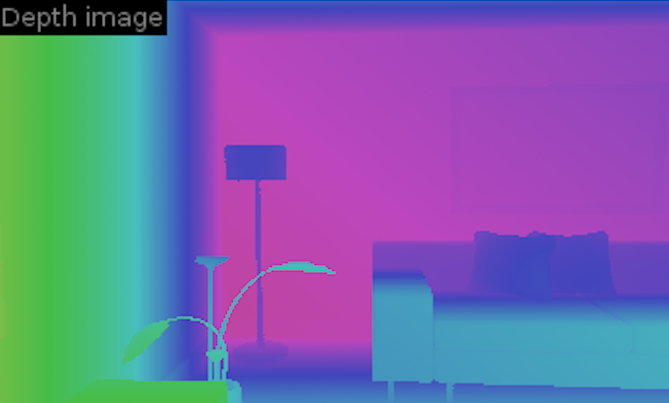
(a) Depth frame captured by an agent

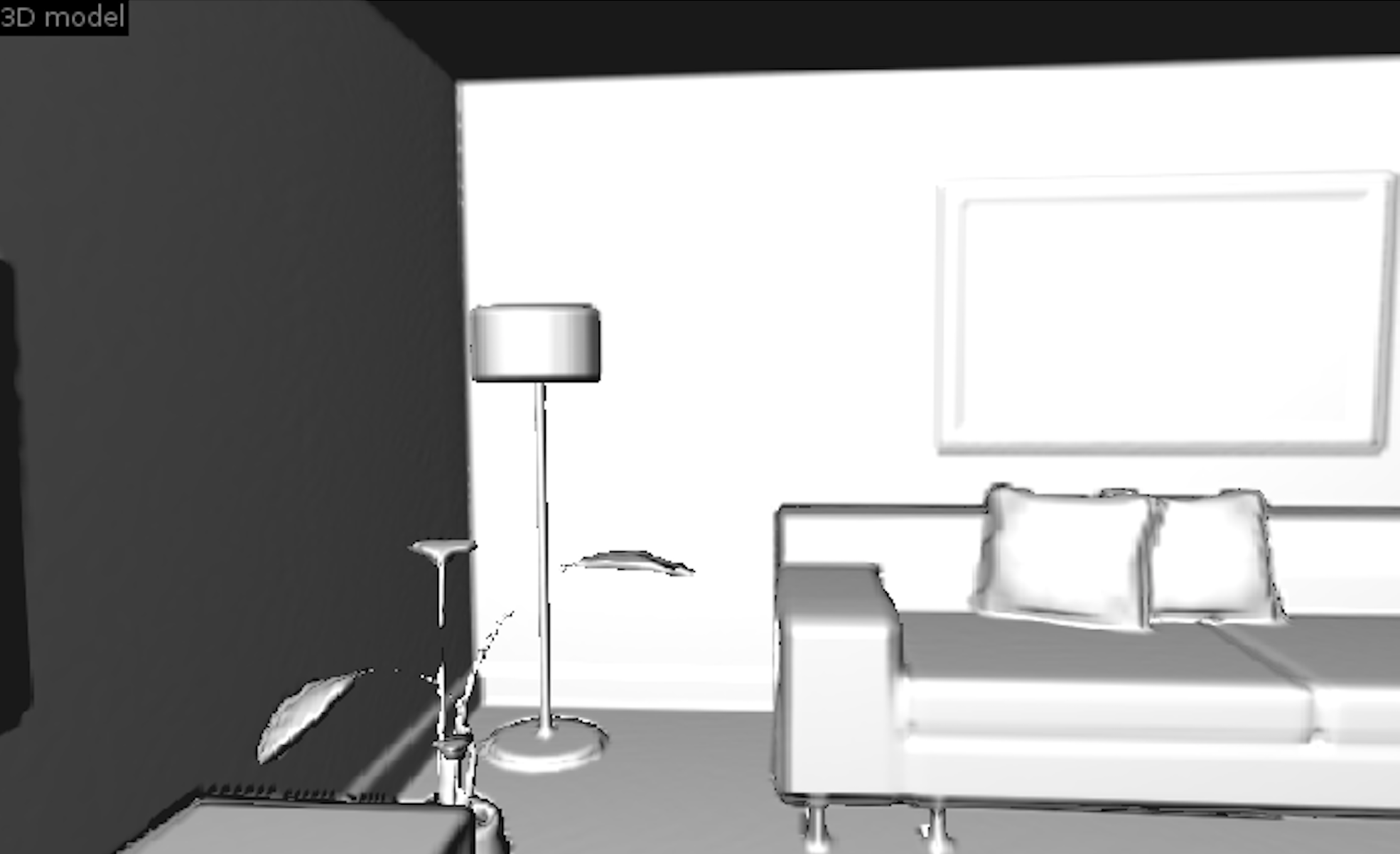
(b) 3D reconstructed surface

Figure 1: KinectFusion takes depth frames as inputs and produces a 3D reconstructed surface with the trajectory of the agent in that environment.

II-A Brief Description of KinectFusion

The KinectFusion algorithm performs the following high-level steps for each input frame [9, 8, 24].

1. Acquisition: an input depth frame such as the one shown in Figure 1a is read in either from a camera or from disk.

2. Preprocessing: depth values in the frame are normalized and a bilateral filter is applied for noise reduction.

3. Localization: a new estimate of the position and orientation (together called a pose) of the camera is computed using the Iterative Closest Point (ICP) algorithm. The algorithm determines the difference in the alignment of the current normalized depth frame with the depth frame computed from the previous camera pose (see raycasting below). This phase is also called tracking in the SLAM literature.

4. Integration: the existing 3D map is updated to incorporate the aligned data for the current frame using the pose determined in the tracking phase.

5. Raycasting: a depth frame from the new camera pose is computed from the global 3D map by raytracing.

6. Rendering: a visualization of the 3D surface is generated, as shown in Figure 1b.

II-B SLAMBench

The SLAMBench [26] implementation of the KinectFusion algorithm exposes the following algorithmic parameters (knobs), which are set to certain default values in SLAMBench.

1. Compute size ratio (csr): resolution of the depth frame used as input.

2. Tracking rate (tr): rate at which tracking and localization are performed.

3. Integration rate (ir): rate at which new frames are integrated to the scene.

4. ICP threshold (icp): threshold for the ICP algorithm.

5. Pyramid level iterations (pd): maximum number of iterations that ICP algorithm can perform on each level of the image pyramid.

6. Volume resolution (vr): resolution at which the scene is reconstructed.

7. $\mu$ distance (mu): the truncation distance in the output volume representation.

These knobs can be tuned to optimize the computation time or energy required for processing each frame. However, this tuning needs to be done under the constraint that the output quality is acceptable since KinectFusion can construct inaccurate 3D maps or trajectories when too much approximation is introduced.

The constraints on output quality are defined as follows. The difference between the actual and the computed location of the agent at any frame is defined as instantaneous trajectory error (ITE). One widely used quality metric used for SLAM is the average trajectory error (ATE), which is the average of the ITE over all the frames of the trajectory. Since ATE is a property of the entire trajectory, it is not known until the end of the trajectory. Furthermore, it requires knowing ground truth (i.e., the actual trajectory taken by the agent), which is usually not available except in simulated SLAM environments. Online control of knobs in SLAM therefore requires a proxy for the ATE that can be computed at each frame rather than at the end of the computation. Section III-B describes the proxy used in SLAMBooster.

II-C Performance of KinectFusion in SLAMBench

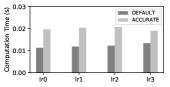
(a) Computation time

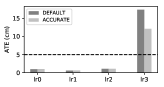
(b) ATE

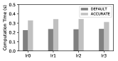
(c) Computation time (in seconds)

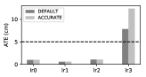
(d) ATE

Figure 2: Performance of the default and the most accurate configurations of KinectFusion. The top row shows performance on an Intel Xeon system, while the bottom row shows performance with an ODROID XU4 system.

To get a sense of the performance of KinectFusion with the default knob settings used in SLAMBench, we ran an unmodified OpenCL implementation of KinectFusion on two platforms with different compute capabilities. The first platform is an Intel Xeon E5-2630 desktop system with a Nvidia Quadro M4000 GPU, and the other is an ODROID XU4 board which is an widely used platform for emulating embedded systems. The ODROID XU4 has an octa-core Exynos 5422 big.LITTLE processor and a Mali-T628 MP6 GPU. The top row in Figure 2 shows the computation time per frame and ATE on the Xeon system, while the bottom row shows these values for the ODROID system. In each figure, the horizontal axis shows four living room trajectories named lr0-lr3 from the ICL-NUIM dataset [33]. The dataset includes ground truth, so it is possible to compute the ATE for these trajectories.

For computation time performance, the vertical axis shows the computation time required by KinectFusion to process each input frame. For the ATE, the vertical axis shows the average deviation between the reconstructed trajectories and the ground truth. In SLAM literature, an ATE of 5 cm or less is considered reasonable [24]; the horizontal dashed lines in Figures 2b and 2d show the 5 cm constraint on the ATE. The left bar, DEFAULT, represents the default settings of the parameters in KinectFusion as set in SLAMBench. ACCURATE represents the most accurate configuration of the parameters for KinectFusion and thus incurs more overhead than DEFAULT. (Note that neither DEFAULT nor ACCURATE can process lr3 well because lr3 has frames that are too difficult to be accurately tracked, so the difference in the amount of error for lr3 introduced by DEFAULT and ACCURATE can be ignored.)

From Figure 2, we see that the best frame rate attainable by KinectFusion on the high-end Xeon system is approximately 90 fps, but it is only 3-4 fps on the big.LITTLE embedded system. Thus, while KinectFusion can achieve real-time processing rates on high-end hardware, it performs poorly on an embedded system with constraints on resources such as hardware capabilities, energy or power consumption, and peak frequency. One way around this problem is to use approximation but this needs to be done without reducing the quality of the output to an unacceptable level. The rest of the paper explores how this is done in SLAMBooster.

III Design Choices in Approximation Controller

In this section, we describe the main choices made in the design of SLAMBooster.

III-A Offline vs. Online Control of Knobs

An offline control system for SLAM would use fixed knob settings for the entire computation, and it would choose the knob settings using cost and error models built from training data, and features of the input trajectory. Offline control has been used successfully to control approximation in long-running compute-intensive programs [34] but there are some obvious drawbacks in using this approach for SLAM. In most applications of SLAM such as robot motion, the environment is discovered while moving through it so the trajectory is not known before the SLAM computation begins. Furthermore, online control permits knob settings to be set adaptively, utilizing information from each frame, and this can be more efficient than setting the knobs once and for all at the start of the SLAM computation. For example, if the scene has objects like chairs or tables, localization and integration are relatively easy and the SLAM computation can be performed with lower precision. Conversely, when the scene has only smooth surfaces like walls, it complicates the process of tracking and aligning frames, and a more precise computation may be needed to avoid large tracking error. A quantitative comparison between online control and offline control is given in Section V-B. For these reasons, SLAMBooster uses online control of approximation.

III-B Proxy for Instantaneous Trajectory Error

An online control system needs online metrics to monitor the performance of the application during execution. As discussed in Section II, the usual error metric used in SLAM is the Average Trajectory Error (ATE) but this is a property of the entire trajectory so it cannot be used directly as an online error estimator. If ground truth is available, we can use the instantaneous trajectory error (ITE) but in most applications of SLAM, ground truth is not available.

To devise a proxy for ITE, we exploit the basic assumption in the KinectFusion algorithm that the movement of the agent between successive frames is small (the algorithm for localization is based on this assumption). To make use of this observation, we evaluated several plausible metrics including the inter-frame difference in depth values and the alignment error as online proxies for error; intuitively, large values of these metrics suggest that the scene is changing suddenly, requiring higher precision computation to avoid large tracking error. However, our experiments showed that there is no strong correlation between these metrics and the ITE. The metric which correlated best with the ITE is the velocity of the agent. The localization phase in the KinectFusion algorithm estimates the pose of the agent, and by looking at the difference in poses between successive frames (assuming every frame is tracked), we can estimate the velocity of the agent. We used Lasso [35] to confirm a positive correlation between the velocity and the ITE for the four ICL-NUIM trajectories for which we have the ground truth. Therefore, we use the estimated velocity of the agent as a proxy for the ITE.

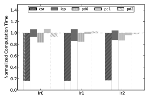
(a) Ranking knobs for computation time

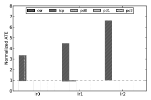
(b) Ranking knobs for ATE

Figure 3: Ranking knobs by importance for ATE and computation time

III-C Reducing the Knob Space

Precise modeling of the relationship between knob settings and computation time or error requires extensive exploration of the knob space and is input-sensitive, which makes it intractable [24]. To make the control problem more tractable, we ignore knobs that are ill-suited for online tuning, such as vr and mu, since they’re input dependent and require recomputing the global map data structure, which is expensive. We also do not control the tracking rate tr or integration rate ir and we set them to one, since every frame should be tracked and integrated in an effort to not violate the assumption that the movement between successive frames is small.

We ranked the remaining knobs by their influence on ATE and computation time. These knobs are csr, icp, and pd. The knob pd has three components, referred to as pd0, pd1, and pd2. Figures 3a and 3b show how computation time and ATE change for the first three living room trajectories from the ICL-NUIM dataset when knobs are changed one at a time, keeping all other knobs fixed at their default values. We find that knobs csr, icp and pd0 have the most impact on performance, and this finding is consistent with prior work [24]. Among the three, csr has dominant impact on computation time and also significantly impacts ATE, which is intuitive since it controls the resolution of the depth image to be used for computation. Knob pd1 and pd2 did not significantly influence ATE or computation time, and hence are less interesting for control. Therefore, we only use csr, icp and pd0 for approximation control in SLAMBooster.

IV SLAMBooster Online Control System

This section describes SLAMBooster in stages. Section IV-A presents a proportional-integral-derivative (PID) controller that controls the knobs identified in Section III-C. This PID controller is successful in reducing computation time and power consumption but it violates the error constraint by a significant margin for some trajectories. Therefore, we improve it by exploiting domain-specific knowledge of the KinectFusion algorithm, using smooth surface detection (Section IV-B) and pose correction (Section IV-C). The computation time performance is further improved by using reduced-precision floating-point operations in some of the computation phases (Section IV-D).

Algorithm 1 Online controller in SLAMBooster for the KinectFusion algorithm applied on each input frame Frame_t.

1:Frame_t $\leftarrow$ KF.acquisition()

2:if $t$ $\leq$ BOOTSTRAP_FRAMES then $\triangleright$ Do not approximate

3:    Knob_t $\leftarrow$ Knob_t-1

4:    Frame_t $\leftarrow$ KF.preprocessing(Frame_t, Knob_t)

5:    Pose_t $\leftarrow$ KF.tracking(Frame_t, Knob_t)

6:    KF.integration(Pose_t, Frame_t, Knob_t)

7:    KF.raycasting(Pose_t, Knob_t)

8:    KF.rendering(Pose_t, Knob_t)

9:else$\triangleright$ Check for approximation opportunities

10:    

11:    Knob_t $\leftarrow$ PID (V_t-1, V_ref) $\triangleright$ PID controller

12:    surface_trigger $\leftarrow$ SurfaceDetection(Frame_t)

13:    if surface_trigger or correction_trigger_t-1 then

14:         Knob_t $\leftarrow$ Knob_t - 1 $\triangleright$ Increase precision

15:    end if

16:    

17:    Frame_t $\leftarrow$ KF.preprocessing(Frame_t, Knob_t)

18:    Pose_t $\leftarrow$ KF.tracking(Frame_t, Knob_t)

19:    

20:    V_t $\leftarrow$ Pose_t - Pose_t-1$\triangleright$ Compute velocity

21:    correction_trigger_t $\leftarrow$ (V_t > CORRECTION_THRES)

22:    if correction_trigger then

23:         Pose_t $\leftarrow$ T_t-1 * Pose_t-1

24:         T_t $\leftarrow$ T_t-1

25:    else

26:         T_t $\leftarrow$ Pose_t * Pose${}_{t-1}^{-1}$

27:    end if

28:    

29:    KF.integration(Pose_t, Frame_t, Knob_t)

30:    KF.raycasting(Pose_t, Knob_t)

31:    KF.rendering(Pose_t, Knob_t)

32:end if

IV-A PID Controller

In its simplest form, a PID controller [36] is like an automobile cruise control - it adjusts knob settings by looking at the difference between a reference value and a value that is derived from the state of the system. This is a proportional (P) controller. To make control more smooth, we can take history into account by considering also the integral (I) of this difference over a time window, and we can make the controller more reactive by considering the derivative (D) of this difference [36].

Algorithm 1 shows the pseudocode for SLAMBooster and incorporates the refinements discussed later in this section. KF in Algorithm 1 stands for KinectFusion, and lines showing operations on KF represent logic from the unmodified KinectFusion algorithm. For simplicity, knobs settings are described in discrete levels. Increasing the level means introducing more approximation, or vice versa. The highlighted code implements optimizations to the baseline controller, and should be ignored for now.

• Line 1 shows an input frame Frame_t is acquired from the I/O device. The rest of Algorithm 1 shows computations performed on Frame_t. Frame pixels are depth values.

• After acquiring the frame, the controller determines whether it is still in the bootstrap phase. No approximation is done for the first few frames to allow KinectFusion to initialize an accurate global 3D map, so the original KinectFusion algorithm is executed (lines 3–8).

• If SLAM is not in the bootstrap phase, the controller picks the knob settings (denoted by Knob_t) based on a PID controller (line 11), which compares the agent’s current velocity (denoted by V_t) and a reference velocity (denoted by V_ref). V_t is estimated using the difference between the poses in the current frame and the previous frame (line 20). The level of the knobs is set proportionately to the difference between V_t and V_ref if V_t is smaller than V_ref. A larger difference means more approximation. When V_t is larger than V_ref, the most accurate knob setting will be applied because higher velocity usually implies higher ITE. After estimated by the proportional (P) part, the knob settings will be further refined by the integral (I) part and the derivative (D) part.

• The I part is a sliding window of the history of V_t and tracks the average velocity over the current window. It adjusts the knob level by comparing the average velocity with a predefined threshold. The length of the velocity window is set to the length of the bootstrap phase. On the other hand, the D part checks whether the velocity is consistently increasing or decreasing over the same sliding window that the I part uses. If the velocity is consistently decreasing, the knob level can be increased to exploit more approximation and vice versa.

Our experiments showed that although this PID controller is effective in reducing the computation time by more than half, it fails to meet the trajectory error constraint for many of our real-world trajectories (see Section V-C). This application-agnostic approach itself is not enough to balance the trade-off between computation time and localization accuracy for the following two reasons:

• This controller does not utilize any information from the input frame. The controller would introduce approximation too aggressively when V_t is low, while low V_t doesn’t necessarily mean that the next frame is easy to track. For example, smooth surfaces are much more difficult to track than scenes with table and chairs.

• For several reasons such as noisy frames, SLAM algorithms may produce a wrong pose that differs substantially from the previous pose. This controller cannot react to such potential incorrect estimations.

Next, we improve the controller by incorporating domain knowledge.

IV-B Smooth Surface Detection

In the tracking and integration phases, KinectFusion merges information from the current depth frame with the global 3D map. Each incoming depth frame in KinectFusion is an abstraction of the scene at which the camera is pointing. If the scene has objects like chairs and tables, it is easier for the algorithm to align and integrate a depth frame with the existing 3D map than if the scene is a blank wall for example. Therefore, it is desirable to adapt the level of approximation to the scene: the smoother the surface is, the more the accuracy that is needed.

The degree of smoothness of a frame is represented by calculating the standard deviations of representative regions of a frame. Lower standard deviation means smoother surfaces. To implement this idea, we sample the four quadrants of the input depth frame, leaving out pixels at the margins of the frame since the Kinect sensor is known to potentially produce invalid depth pixels at the periphery (Figure 4). To reduce computational overhead, a fixed number of pixels are sampled from each quadrant, independent of the resolution of the frame; this number is chosen so that at the lowest resolution, all pixels are sampled. At the second lowest resolution, every other pixel is sampled, etc. We then compute the standard deviation of depth values within each quadrant. If all these standard deviations are below some threshold value, the camera might be pointing to a smooth surface so the control system increases the precision of KinectFusion computation.

Figure 4: Smooth surface detection heuristic. We compute the intra-sample deviation from samples in the depth image.

Algorithm 1 shows the augmented control system using smooth surface detection. The SurfaceDetection function implements smooth surface detection (line 12, Figure 4). This additional information is used by the controller to manipulate knobs (line 13). Our experiments indicate that compared with the PID controller, this improves the ATE with little additional computation overhead.

IV-C Pose Correction

The final enhancement we make to the basic PID control system is to use a simple form of Kalman filtering [37, 38] to recompute the pose when it appears that the agent has made a sudden movement. Informally, Kalman filtering is a method for combining a number of uncorrelated estimates of some unknown quantity to obtain a more reliable estimate. In many practical problems, the unknown quantity is the state of a dynamical system, and there are two estimates of this state at each time step, one from a model of state evolution and one from measurement, that are combined using Kalman filtering.

In the context of SLAM, the unknown state is the pose of the agent. When a frame is processed by KinectFusion, the tracking module uses the measured depth values in the frame to provide an estimate of the new pose, as shown in line 18 in Algorithm 1. However, if this estimated pose differs substantially from the pose in the previous frame, it violates the assumption that the movement of the agent between successive frames should be small. This indicates that KinectFusion has potentially inferred an inaccurate pose, and the pose estimate from the tracking module may be unreliable.

In the spirit of Kalman filtering, we use a simple model to estimate the pose if the estimate from the measurement produced by the tracking module is substantially different from the pose in the previous frame. Lines 22–27 in Algorithm 1 show the pseudocode. KinectFusion represents the live 6DOF camera pose estimate by a rigid body transformation matrix. T_t-1 represents the transformation matrix calculated at frame $t-1$ when Pose_t-1 is computed from Pose_t-2. The logic compares $V_{t}$ with a threshold to check whether correcting Pose_t is required. If the velocity is below the threshold, the matrix T_t will be calculated using the current and the previous pose. On the other hand, if the difference in poses is abnormally large, Pose_t is recomputed by applying T_t-1 to Pose_t-1, following the assumption that the movement between successive frames should be small. Downstream KinectFusion kernels work using this corrected estimate of Pose_t.

Section V-C shows that correcting pose estimations in this way improves the accuracy of the trajectory reconstruction substantially, with minimal control overhead.

IV-D Reduced-precision Floating-point Format

Finally, we explored the benefit of using half-precision floating-point numbers instead of the default single-precision floating-point numbers. Half-precision format can potentially improve vector operation efficiency and cache miss rates. OpenCL extension cl_khr_fp16 has support for half scalar and vector types as built-in types that can be used for arithmetic operations, type casts, etc.

Some phases in KinectFusion such as Localization and Integration have constants that are too small to be represented in half-precision format. Therefore, we manually transformed only the Raycasting and Preprocessing phases to use half-precision format. Since these phases perform a large number of vector operations, use of reduced precision can be beneficial [25].

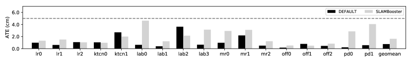
(a) Absolute ATE.

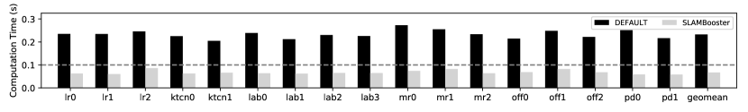
(b) Average Computation Time Per Frame.

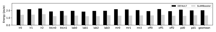
(c) Average Energy Consumption Per Frame.

Figure 5: ATE, computation time and energy performance on embedded platform

V Experimental Results

This section evaluates the benefits and effectiveness of SLAMBooster for approximating KinectFusion.

V-A Methodology

We implemented SLAMBooster in the open-source SLAMBench [26] infrastructure.

Platform

Figure 2 shows that unmodified KinectFusion achieves good performance ($\sim$90 fps) on a high-end Intel Xeon E5-2630 system with a Nvidia Quadro M4000 GPU. Our experiments with the Intel Xeon system show that SLAMBooster is able to improve the performance further ($\sim$200 fps) without failing the accuracy constraint. We do not show results with the Intel Xeon system for lack of space. Instead, we present detailed results with SLAMBooster on a low-power embedded environment using an ODROID XU4 board with a Samsung Exynos 5422 octa-core processor. The Exynos processor has four Cortex-A15 cores running at 2 GHz and four Cortex-A7 cores running at 1.4 GHz, and has 2 GB LPDDR3 RAM. The XU4 board is equipped with a Mali-T628 MP6 GPU that supports OpenCL 1.2, and runs Ubuntu 16.04.4 LTS with Linux Kernel 4.14 LTS. The XU4 board does not have on-board power monitors, we use a SmartPower2 device to monitor energy consumption for the whole board.

Benchmark trajectories

SLAMBench supports the ICL-NUIM RGB-D living room dataset, which is used for benchmarking SLAM algorithms [33]. This dataset is obtained by using the Kintinuous system [10] with ground truth trajectory. Each scene has several synthetically-generated trajectories. We excluded benchmark lr3 from our experiments since even the ACCURATE configuration cannot meet the error constraint (Figure 2). Therefore, we use three trajectories with the living room scene, referred to as lr0, lr1 and lr2 in this paper.

To increase the diversity of trajectories, we used a first-generation Kinect camera to collect fourteen additional trajectories from real-world scenes in an indoor environment. The fourteen trajectories are: ktcn0, ktcn1, lab0, lab1, lab2, lab3, mr0, mr1, mr2, off0, off1, off2, pd0, and pd1. All the inputs are collected at 30 fps with resolution 640x480. We do not have ground truth for these trajectories, hence we use the trajectory computed by the most accurate setting of KinectFusion as a stand-in for ground truth. We have verified using SLAMBench GUI that KinectFusion is able to rebuild the trajectories and 3D map correctly. Column 2 in Table I shows the length of each trajectory.

The extended SLAMBench implementation and collected trajectories will be made publicly available when the paper is published.

V-B Performance of SLAMBooster

Figure 5 shows the ATE, average computation time per frame, and average energy consumption per frame for the benchmark trajectories on the embedded platform. The figures compare two configurations: using the default knob settings in SLAMBench, and using SLAMBooster to control knobs online. Each bar is the average of three trials. Performance numbers are shown in a tabular form in Table I.

For most trajectories, ATE is higher when knobs are controlled with SLAMBooster, as expected. Nevertheless, all individual ATEs are less than 5 cm and therefore meets the required quality constraint. Figure 5b shows the average computation time for each frame. The average speedup of SLAMBooster over DEFAULT is 3.6x and achieves a throughput of 15 fps. Although this frame rate does not meet real time constraint, computer graphics researchers consider 15 fps to be reasonable for providing smooth user experience.

Figure 5c shows another important metric, the average energy consumed for processing a frame. The idle power dissipation of an ODROID XU4 board is about $\sim$4 Watt. The energy saving for each frame is about $\sim$35%. The reduction in energy per frame is not as significant as the reduction in computation time per frame because of the frequent up and down scaling of certain data structures, required while tuning the csr knob.

Control overhead

The overhead of SLAMBooster arises mainly from data structure down sampling and up sampling when tuning knob csr. Measurements show that the average overhead introduced by the controller is $\sim$1 ms on ODROID XU4 board, which is $\sim$1% of the total computation time. Therefore, the overhead of the control logic is negligible.

		Default KinectFusion				SLAMBooster
	# frames		Comp.	ATE	Energy (J)/		Comp.	ATE	Energy (J)/
			time (ms)	(cm)	frame		time (ms)	(cm)	frame
lr0	1510		235	0.98	2.13		62	1.30	1.41
lr1	967		234	0.61	2.19		60	1.51	1.44
lr2	882		246	1.07	2.28		86	1.03	1.50
ktcn0	1550		225	1.05	1.87		63	0.97	1.23
ktcn1	800		204	2.70	1.94		66	2.00	1.31
lab0	800		239	0.63	1.96		64	4.62	1.30
lab1	1250		212	0.39	1.85		62	1.21	1.22
lab2	1250		230	3.63	1.95		65	2.14	1.23
lab3	1250		226	0.65	1.96		65	3.14	1.35
mr0	929		273	0.97	2.18		74	2.93	1.28
mr1	1494		255	2.19	2.15		82	3.10	1.31
mr2	1450		236	0.49	2.06		64	1.22	1.33
off0	750		215	0.17	1.92		69	0.52	1.33
off1	1050		248	0.78	2.20		82	0.49	1.41
off2	1200		221	0.45	1.91		68	0.83	1.28
pd0	1600		251	0.21	2.12		59	2.85	1.26
pd1	1500		216	0.57	2.01		58	4.06	1.34
geomean			232	0.75	2.04		67	1.63	1.32

TABLE I: Detailed results with input trajectories controlled by the SLAMBooster on the ODROID XU4 platform.

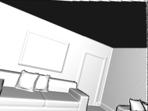
(a) 3D surface reconstructed by ACCURATE

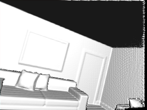
(b) 3D surface reconstructed by SLAMBooster

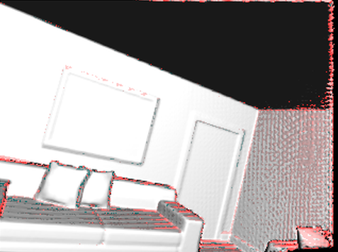
(c) 3D surface difference

Figure 6: Evaluation of the quality of 3D maps

3D map comparison

Since SLAM is used for navigation, the 3D map is mainly a mean to an end rather than an end in itself; nevertheless it is interesting to study the quality of the 3D map produced by SLAMBooster. Figure 6 compares a typical global 3D map built by using the most accurate knob settings (Figure 6a) with the one built by using SLAMBooster (Figure 6b). Figure 6c is a diff of these two maps in which pixels that are substantially different are marked in red. We see that using SLAMBooster does not impact the quality of the 3D map substantially.

Use only csr in control

Since knob csr dominates the knob space, it is interesting to see how the controller performs without knob icp and pd0. Our experiment shows that the saving in computation time and energy with only csr is 58% and 29% respectively, compared to 72% and 35% with icp and pd0. Having more knobs in the controller helps improve the performance of SLAMBooster.

V-C Impact of Optimizations

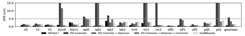
(a) Absolute ATE.

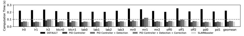
(b) Average Computation Time Per Frame.

Figure 7: Incremental optimization impact on ATE and computation time

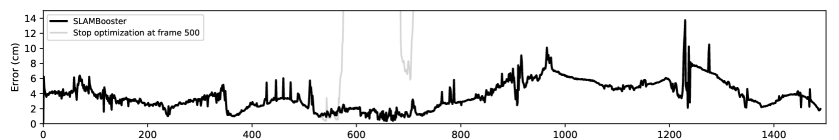
(a) Trajectory Error

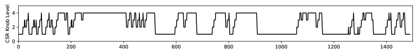
(b) Knob Activity: csr

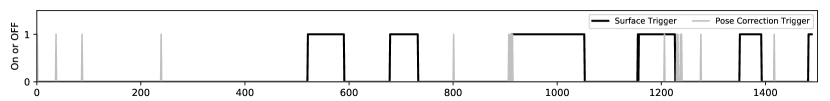
(c) Trigger Activity: Surface Trigger and Pose Correction Trigger

Figure 8: Trajectory error, knob activity and trigger activity in chronological order for benchmark: mr1

Figure 7 shows the incremental impact of the different optimizations on the PID controller. The controller configurations are listed below.

• DEFAULT setting provided by SLAMBench

• PID control

• PID control + smooth surface detection

• PID control + smooth surface detection + pose correction

• SLAMBooster: PID control + smooth surface detection + pose correction + half-precision floating point

Figures 7a and 7b show the ATE and computation time respectively for the different controller configurations. The PID controller by itself achieves much of the time savings but violates the error constraint for 5 out of 17 inputs. This is not acceptable since nearly a third of the inputs fail to meet the error constraint. When the smooth surface detection is incorporated into the controller, the overall error performance is improved, but 4 inputs still fail to meet the 5 cm error constraint. Note that surface detection introduces a $\sim$15% computation time overhead compared to the PID controller.

When pose correction is incorporated, all the benchmarks meet the error constraint. It is interesting to note that this reduces the overall computation time compared to using only smooth surface detection. The reason is that this setting improves localization and mapping, so more approximation can be done safely, leading to reduced computation time. Finally, when half-precision floating-point arithmetic is added, the overall computation time is improved by $\sim$5% at the cost of slightly worse error. Note that for a few of the trajectories, SLAMBooster produces less ATE than "PID controller + Detection + Correction" does. This is because KinectFusion is highly non-linear, so the reduction in precision may affect the results in a positive way.

V-D Effectiveness of Online Control

The results in the previous section showed the effectiveness of SLAMBooster for entire trajectories. To get a better sense of how online control in SLAMBooster works, it is useful to visualize how knob settings change from the beginning to the end of a complete trajectory. Figure 8 is such a visualization for the mr1 trajectory, which is one of the most difficult trajectories in our benchmark set. The PID controller, even with smooth surface detection, fails to meet the error constraint. In Figure 8, the $x$ axis represents frame number in chronological order.

The black line in Figure 8a shows instantaneous trajectory error (ITE) over time when SLAMBooster is used for the entire trajectory. Those ITEs are computed after the execution by comparing the reconstructed trajectory with the ground truth, which is assumed to be the trajectory reconstructed with the most accurate setting of KinectFusion. Figure 8b and Figure 8c show the settings of the csr knob and the activation of smooth surface triggers and pose correction triggers respectively.

To demonstrate the effectiveness of SLAMBooster, we show another configuration in Figure 8a (represented by the gray line). In this configuration, we switch SLAMBooster to the PID controller after frame 500. During frames 520–590, the camera encounters a smooth surface and the PID controller cannot deal with it by itself. As shown in Figure 8a, ITE increases dramatically (peak ITE is $\sim$100 cm and is too large to be plotted on this scale) and never comes down to an acceptable level. This shows that the optimization techniques used in SLAMBooster are critical for complex trajectories like mr1.

Figure 8b shows the activity of the most important knob csr. Frames 200 to 400 are relatively easy and speed is low, so SLAMBooster tunes the knob all the way up to approximate the computation. For frames between 700 to 1200, ITE gets larger because the velocity of the agent increases. As a result, csr is set to the most accurate value by SLAMBooster in order to handle the drift in the trajectory.

This example shows that SLAMBooster can control the knobs dynamically to exploit opportunities to save computation time and energy while ensuring that the localization error is within some reasonable bound.

V-E PID Controller vs. Hierarchical Step Controller

As discussed in Section V-B, the energy saving of SLAMBooster is not as good as its saving in computation time. The potential reason is that the PID controller in SLAMBooster frequently changes knob csr, causing certain data buffers within the SLAM algorithm to be scaled up and down frequently.

To explore this issue, we designed a variant of SLAMBooster, with a hierarchical step controller as an alternative to the PID controller. Instead of generating exact knob settings, the hierarchical step controller only generates two signals: increase or decrease approximation. Signals are generated by comparing velocity and average velocity to predefined thresholds, and checking whether the velocity is ascending or descending, similar to the PID controller. Instead of tuning multiple knobs simultaneously, a hierarchical step controller tunes only one knob one level at a time, following the order of importance of the knobs discussed in Section III-C. Other optimizations like surface detection, pose correction, and reduced-precision floating-point computation are the same in the design variant.

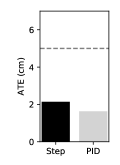
(a)

(b)

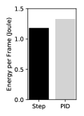
(c)

Figure 9: SLAMBooster with PID controller or hierarchical step controller.

Figure 9 compares the performance of the two controllers. Though the step controller version SLAMBooster spends 29% more computation time than the PID version, it uses 12% less energy. The saving in energy can be explained by the fact that the tuning of the knob settings become smoother with the hierarchical step controller. However, the longer reaction time to get to ideal knob setting hurts its computation time.

V-F Comparison with Other Control Strategies

This section compares SLAMBooster with controllers based on two very different design philosophies: offline control and application-agnostic control.

Comparison with offline control

We compare the performance of SLAMBooster with offline control, given the best offline knob setting of each trajectory. The best offline knob setting is conducted by exhaustively searching the knob space described in Section III-C for each input with the same error bound. On average, SLAMBooster is 1.32x faster than offline control. Interestingly, SLAMBooster is 1.39x faster for real world inputs while the best offline knob setting is slightly faster (3%) for synthetic inputs (lr0, lr1, lr2). The reason is that SLAMBooster is designed for general inputs whereas synthetic inputs are generally easier to process.

Comparison with application-agnostic control

We compare SLAMBooster with an application-agnostic control system for software applications. Application-agnostic control systems have been used successfully in the literature to control a diverse set of applications [39, 30]. Next, we first briefly present a general strategy to design such a control system, which we call TC, and then describe our adaptions to SLAM.

• The application execution is divided into intervals or windows of some size (e.g., 32 or 64 frames in our experiments). TC tries to meet the desired performance constraints and objectives on the average for each window.

• In each interval, TC tracks how well the performance constraint has been met, and this information is used to decide whether the system should be sped up or slowed down in the next interval to better meet the performance constraint. This desired performance level is normalized by the performance obtained by setting knobs to their default values, and this dimensionless quantity ("performance speedup") is used to find the knobs for the next interval.

• To find knob settings for a desired performance speedup, TC consults a configuration table, which returns Pareto optimal knob settings for a given performance speedup (in some cases, it returns a pair of knob configurations but this detail can be ignored). The configuration table is constructed ahead of time by profiling the program using representative inputs and knob configurations.

We implemented an online controller for SLAM following the traditional control design scheme described above. Instead of a performance speedup requirement, each time interval is given an error budget (i.e., the total amount of error allowed in the next interval) whose value is computed using TC’s strategy for determining performance speedup. Since ground truth is not available for most of our trajectories, we use velocity as a proxy for the actual error in each interval (a reference velocity is defined as the required velocity). The base velocity for each window, corresponding to the base performance in the original traditional controller, is provided by ground truth instead of implementing Kalman filtering [30]. Note that this value is at least as accurate as what Kalman filtering estimates. We used two approaches to build the configuration table. The first one used the three synthetically-generated living room trajectories lr0, lr1 and lr2 for profiling. Since these trajectories are not representative of the entire set of trajectories in our benchmark set, we would expect the performance of the controller to be poor. The second approach is to use a more diverse set of inputs, one from each scene in the benchmark set (for example, mr1 is picked from the meeting room category).

	Living Rooms Config		Diverse Rooms Config
Ref	# Error	# Better	# Error	# Better
Velocity	Violated	Time	Violated	Time
0.004	3.5	1	1	0
0.005	5.5	2	1	0
0.006	7	3	1	0
0.008	10	3	2	0
0.010	10	5	2	0
0.012	10	6	2	0

TABLE II: Traditional online controller performance

Table II shows the performance of the traditional control scheme compared to SLAMBooster. The evaluation includes running all the benchmarks using the traditional controller on each configuration table with different values for the reference velocity. The Error Violated column shows the number of inputs that violate the 5 cm error constraint, while the Better Time column shows the number of trajectories that satisfy the error constraint and have less computation time than with SLAMBooster. When the configuration table is built using only the living room trajectories (Living Rooms Config), the controller introduces approximation too aggressively because the profiling set, living room trajectories (lr0, lr1, lr2), are relatively simple to approximate comparing to other real world trajectories. When the error budget (reference velocity) gets looser, more trajectories achieve better computation time at the cost of unacceptable tracking error. On the other hand, when profiling is done with the diverse trajectory set (Diverse Rooms Config), the error constraint is rarely violated but the computation times are slower than with SLAMBooster because the configuration table is overly conservative.

Prior work has shown that a traditional controller can control a diverse set of applications [30, 39]. However, high input sensitivity and low error tolerance characteristic of SLAM makes it difficult for a traditional controller to control KinectFusion. Intuitively, the configuration table is a model of system behavior that averages over all the trajectories used in the profiling (training) phase, so the controller cannot optimize the behavior of the system for the particular trajectory of interest in a given execution. In addition, this controller does not exploit the SLAM-specific techniques in SLAMBooster such as smooth surface detection and pose correction, which proved essential in Section V-D.

VI Related Work

We discuss work on approximation in SLAM algorithms and on using control-theoretic approaches for optimal resource management.

VI-A Approximating SLAM

Recent work has used KinectFusion and the SLAMBench infrastructure to study the performance impact of reduced-precision floating-point arithmetic in SLAM algorithms [25, 40]. Unlike SLAMBooster, these approaches do not exploit approximation at the algorithmic level.

Offline control of KinectFusion has been explored by Bodin et al.[24] using an active learning technique. Given the entire trajectory ahead of time, they use a random forest of decision trees to characterize the input trajectory, and generate a Pareto optimal set of configurations that trades off computation time, energy consumption and the ATE. In addition to algorithmic knobs, they also explore approximation of compiler and hardware-level knobs. Their study is limited to a subset of frames for one synthetically-generated trajectory. Follow-up work utilizes the motion information of the autonomous agent to improve offline control and evaluates the offline approximation technique on other SLAM algorithms [41, 27]. In contrast, SLAMBooster performs online control so it does not need to know the entire trajectory before the agent begins to move. Adaptive control of knobs also permits SLAMBooster to optimize knob settings dynamically to take advantage of diverse environments, which is not possible with offline control.

VI-B Adaptive Resource Management

Several systems have been proposed that aim to balance power or energy consumption along with performance and program accuracy [28, 29, 30, 31]. Rumba is an online quality management system for detection and correction of large approximation errors in an approximate accelerator-based computing environment. Rumba applies lightweight checks during the execution to detect large approximation errors and then fixes these errors by exact re-computation [31]. However, recomputation is not feasible in the context of SLAM algorithms because it takes a stream of frame as input and the result of SLAM is used for real-time control. JouleGuard is a runtime control system that coordinates approximate applications with system resource usage to provide control-theoretic guarantees on energy consumption (i.e., will not exceed a given threshold), while maximizing accuracy [28]. The control system uses reinforcement learning to identify the most energy-efficient configuration, and uses an adaptive PID controller-like mechanism to maintain application accuracy. POET measures program progress and power consumption, uses feedback control theory to ensure the timing goals are met, and solves a linear optimization problem to select minimal energy resource allocations based on a user-provided specification [30]. MeanTime is a approximation system for embedded hardware that uses control theory for resource allocation [29]. These techniques combine PID-like control techniques to various parts of the system, and provide empirical demonstrations of overall system behavior without taking domain knowledge into consideration. Recent work on optimal resource allocation focuses on designing sophisticated control systems using linear quadratic Gaussian control for example [42, 43, 44]. Unlike SLAMBooster, they also do not exploit application-specific properties to perform control.

VII Conclusion

SLAM algorithms are increasingly being deployed in low-power systems but a big obstacle to widespread adoption of SLAM is its computational expense. In this work, we present SLAMBooster, a PID control system, to approximate the computation in KinectFusion, which is a popular dense SLAM algorithm. We show that the SLAMBooster, augmented with insights from the application domain, is effective in reducing the computation time and the energy consumption, with acceptable bounds on the localization accuracy.

References

- [1] S. Sidiroglou-Douskos, S. Misailovic, H. Hoffmann, and M. Rinard, “Managing Performance vs. Accuracy Trade-offs With Loop Perforation,” in Proceedings of the 19th ACM SIGSOFT Symposium and the 13th European Conference on Foundations of Software Engineering, ser. ESEC/FSE ’11. New York, NY, USA: ACM, 2011, pp. 124–134.
- [2] M. Samadi, D. A. Jamshidi, J. Lee, and S. Mahlke, “Paraprox: Pattern-Based Approximation for Data Parallel Applications,” in Proceedings of the 19th International Conference on Architectural Support for Programming Languages and Operating Systems, ser. ASPLOS ’14. New York, NY, USA: ACM, 2014, pp. 35–50.
- [3] M. Carbin, D. Kim, S. Misailovic, and M. C. Rinard, “Proving Acceptability Properties of Relaxed Nondeterministic Approximate Programs,” in Proceedings of the 33rd ACM SIGPLAN Conference on Programming Language Design and Implementation, ser. PLDI ’12. New York, NY, USA: ACM, 2012, pp. 169–180.
- [4] M. Carbin, S. Misailovic, and M. C. Rinard, “Verifying Quantitative Reliability for Programs That Execute on Unreliable Hardware,” in Proceedings of the 2013 ACM SIGPLAN International Conference on Object Oriented Programming Systems Languages & Applications, ser. OOPSLA ’13. New York, NY, USA: ACM, 2013, pp. 33–52.
- [5] J. Park, H. Esmaeilzadeh, X. Zhang, M. Naik, and W. Harris, “FlexJava: Language Support for Safe and Modular Approximate Programming,” in Proceedings of the 2015 10th Joint Meeting on Foundations of Software Engineering, ser. ESEC/FSE 2015. New York, NY, USA: ACM, 2015, pp. 745–757.
- [6] A. Sampson, W. Dietl, E. Fortuna, D. Gnanapragasam, L. Ceze, and D. Grossman, “EnerJ: Approximate Data Types for Safe and General Low-Power Computation,” in Proceedings of the 32Nd ACM SIGPLAN Conference on Programming Language Design and Implementation, ser. PLDI ’11. New York, NY, USA: ACM, 2011, pp. 164–174.
- [7] A. Sampson, P. Panchekha, T. Mytkowicz, K. S. McKinley, D. Grossman, and L. Ceze, “Expressing and Verifying Probabilistic Assertions,” in Proceedings of the 35th ACM SIGPLAN Conference on Programming Language Design and Implementation, ser. PLDI ’14. New York, NY, USA: ACM, 2014, pp. 112–122.
- [8] S. Izadi, D. Kim, O. Hilliges, D. Molyneaux, R. Newcombe, P. Kohli, J. Shotton, S. Hodges, D. Freeman, A. Davison, and A. Fitzgibbon, “KinectFusion: Real-time 3D Reconstruction and Interaction Using a Moving Depth Camera,” in Proceedings of the 24th annual ACM symposium on User interface software and technology. ACM, Oct. 2011, pp. 559–568.
- [9] R. A. Newcombe, S. Izadi, O. Hilliges, D. Molyneaux, D. Kim, A. J. Davison, P. Kohli, J. Shotton, S. Hodges, and A. Fitzgibbon, “KinectFusion: Real-Time Dense Surface Mapping and Tracking,” in IEEE ISMAR. IEEE, Oct. 2011.
- [10] T. Whelan, J. Mcdonald, M. Kaess, M. Fallon, H. Johannsson, and J. J. Leonard, “Kintinuous: Spatially Extended KinectFusion,” in 3rd RSS Workshop on RGB-D: Advanced Reasoning with Depth Cameras, 2012.
- [11] R. Mur-Artal, J. M. M. Montiel, and J. D. Tardøs, “ORB-SLAM: A Versatile and Accurate Monocular SLAM System,” IEEE Transactions on Robotics, vol. 31, no. 5, pp. 1147–1163, Oct. 2015.
- [12] S. Borthwick and H. Durrant-Whyte, “Simultaneous Localisation and Map Building for Autonomous Guided Vehicles,” in Intelligent Robots and Systems ’94. ’Advanced Robotic Systems and the Real World’, IROS ’94. Proceedings of the IEEE/RSJ/GI International Conference on, vol. 2, Sep. 1994, pp. 761–768 vol.2.
- [13] T. Whelan, S. Leutenegger, R. S. Moreno, B. Glocker, and A. Davison, “ElasticFusion: Dense SLAM Without A Pose Graph,” in Proceedings of Robotics: Science and Systems, Rome, Italy, Jul. 2015.
- [14] J. Engel, T. Schöps, and D. Cremers, “Lsd-slam: Large-scale direct monocular slam,” in European conference on computer vision. Springer, 2014, pp. 834–849.
- [15] K. Tateno, F. Tombari, I. Laina, and N. Navab, “Cnn-slam: Real-time dense monocular slam with learned depth prediction,” in Proceedings of the IEEE Conference on Computer Vision and Pattern Recognition, 2017, pp. 6243–6252.
- [16] O. Kähler, V. A. Prisacariu, C. Y. Ren, X. Sun, P. Torr, and D. Murray, “Very high frame rate volumetric integration of depth images on mobile devices,” IEEE transactions on visualization and computer graphics, vol. 21, no. 11, pp. 1241–1250, 2015.
- [17] S. Leutenegger, S. Lynen, M. Bosse, R. Siegwart, and P. Furgale, “Keyframe-based visual–inertial odometry using nonlinear optimization,” The International Journal of Robotics Research, vol. 34, no. 3, pp. 314–334, 2015.
- [18] K. Boikos and C. S. Bouganis, “Semi-Dense SLAM on an FPGA SoC,” in 2016 26th International Conference on Field Programmable Logic and Applications (FPL), Aug. 2016, pp. 1–4.
- [19] A. Ratter, C. Sammut, and M. McGill, “GPU Accelerated Graph SLAM and Occupancy Voxel Based ICP for Encoder-Free Mobile Robots,” in 2013 IEEE/RSJ International Conference on Intelligent Robots and Systems, Nov. 2013, pp. 540–547.
- [20] A. J. Davison, I. D. Reid, N. D. Molton, and O. Stasse, “Monoslam: Real-time single camera slam,” IEEE Transactions on Pattern Analysis & Machine Intelligence, no. 6, pp. 1052–1067, 2007.
- [21] G. Klein and D. Murray, “Parallel tracking and mapping for small ar workspaces,” in Proceedings of the 2007 6th IEEE and ACM International Symposium on Mixed and Augmented Reality. IEEE Computer Society, 2007, pp. 1–10.
- [22] C. Forster, M. Pizzoli, and D. Scaramuzza, “Svo: Fast semi-direct monocular visual odometry,” in 2014 IEEE international conference on robotics and automation (ICRA). IEEE, 2014, pp. 15–22.
- [23] R. Sim, P. Elinas, M. Griffin, J. J. Little et al., “Vision-based slam using the rao-blackwellised particle filter,” in IJCAI Workshop on Reasoning with Uncertainty in Robotics, vol. 14, no. 1, 2005, pp. 9–16.
- [24] B. Bodin, L. Nardi, M. Z. Zia, H. Wagstaff, G. Sreekar Shenoy, M. Emani, J. Mawer, C. Kotselidis, A. Nisbet, M. Lujan, B. Franke, P. H. Kelly, and M. O’Boyle, “Integrating Algorithmic Parameters into Benchmarking and Design Space Exploration in 3D Scene Understanding,” in Proceedings of the 2016 International Conference on Parallel Architectures and Compilation, ser. PACT ’16. New York, NY, USA: ACM, 2016, pp. 57–69.
- [25] O. Palomar, A. Nisbet, J. Mawer, G. Riley, and M. Lujan, “Reduced precision applicability and trade-offs for SLAM algorithms,” in Third Workshop on Approximate Computing, ser. WACAS, 2017.
- [26] L. Nardi, B. Bodin, M. Z. Zia, J. Mawer, A. Nisbet, P. H. J. Kelly, A. J. Davison, M. Luján, M. F. P. O’Boyle, G. Riley, N. Topham, and S. Furber, “Introducing SLAMBench, a performance and accuracy benchmarking methodology for SLAM,” in IEEE International Conference on Robotics and Automation (ICRA), May 2015, arXiv:1410.2167.
- [27] S. Saeedi, L. Nardi, E. Johns, B. Bodin, P. Kelly, and A. Davison, Application-oriented Design Space Exploration for SLAM Algorithms. IEEE, Jul. 2017, pp. 5716–5723.
- [28] H. Hoffmann, “JouleGuard: Energy Guarantees for Approximate Applications,” in Proceedings of the 25th Symposium on Operating Systems Principles, ser. SOSP ’15. New York, NY, USA: ACM, 2015, pp. 198–214.
- [29] A. Farrell and H. Hoffmann, “MEANTIME: Achieving Both Minimal Energy and Timeliness with Approximate Computing,” in 2016 USENIX Annual Technical Conference (USENIX ATC 16). Denver, CO: USENIX Association, Jun. 2016, pp. 421–435. [Online]. Available: https://www.usenix.org/conference/atc16/technical-sessions/presentation/farrell
- [30] C. Imes, D. H. K. Kim, M. Maggio, and H. Hoffmann, “POET: A Portable Approach to Minimizing Energy Under Soft Real-time Constraints,” in 21st IEEE Real-Time and Embedded Technology and Applications Symposium, Apr. 2015, pp. 75–86.
- [31] D. S. Khudia, B. Zamirai, M. Samadi, and S. Mahlke, “Rumba: An online quality management system for approximate computing,” in 2015 ACM/IEEE 42nd Annual International Symposium on Computer Architecture (ISCA). IEEE, 2015, pp. 554–566.
- [32] T. Whelan, M. Kaess, H. Johannsson, M. Fallon, J. J. Leonard, and J. McDonald, “Real-time large-scale dense rgb-d slam with volumetric fusion,” The International Journal of Robotics Research, vol. 34, no. 4-5, pp. 598–626, 2015.
- [33] A. Handa, T. Whelan, J. McDonald, and A. J. Davison, “A Benchmark for RGB-D Visual Odometry, 3D Reconstruction and SLAM,” in 2014 IEEE International Conference on Robotics and Automation (ICRA), May 2014, pp. 1524–1531.
- [34] X. Sui, A. Lenharth, D. S. Fussell, and K. Pingali, “Proactive Control of Approximate Programs,” in Proceedings of the Twenty-First International Conference on Architectural Support for Programming Languages and Operating Systems, ser. ASPLOS ’16. New York, NY, USA: ACM, 2016, pp. 607–621.
- [35] R. Tibshirani, “Regression Shrinkage and Selection via the Lasso,” Journal of the Royal Statistical Society, vol. 58, no. 1, pp. 267–288, 1996.
- [36] N. Nise, Control systems engineering. Wiley Interscience, 1994.
- [37] M. S. Grewal and A. P. Andrews, Kalman Filtering: Theory and Practice with MATLAB, 4th ed. Wiley-IEEE Press, 2014.
- [38] Yan Pei, Swarnendu Biswas, Donald S. Fussell, and Keshav Pingali, “An Elementary Introduction to Kalman Filtering,” ArXiv e-prints, Oct. 2017.
- [39] A. Filieri, H. Hoffmann, and M. Maggio, “Automated Design of Self-adaptive Software with Control-Theoretical Formal Guarantees,” in Proceedings of the 36th International Conference on Software Engineering, ser. ICSE 2014. New York, NY, USA: ACM, 2014, pp. 299–310.
- [40] J. Oh, J. Choi, G. C. Januario, and K. Gopalakrishnan, “Energy-efficient simultaneous localization and mapping via compounded approximate computing,” in Signal Processing Systems (SiPS), 2016 IEEE International Workshop on. IEEE, 2016, pp. 51–56.
- [41] L. Nardi, B. Bodin, S. Saeedi, E. Vespa, A. J. Davison, and P. H. J. Kelly, “Algorithmic Performance-Accuracy Trade-off in 3D Vision Applications Using HyperMapper,” ArXiv e-prints, Feb. 2017.
- [42] R. P. Pothukuchi, A. Ansari, P. Voulgaris, and J. Torrellas, “Using Multiple Input, Multiple Output Formal Control to Maximize Resource Efficiency in Architectures,” in Proceedings of the 43rd International Symposium on Computer Architecture, ser. ISCA ’16. Piscataway, NJ, USA: IEEE Press, 2016, pp. 658–670. [Online]. Available: https://doi.org/10.1109/ISCA.2016.63
- [43] N. Mishra, C. Imes, J. D. Lafferty, and H. Hoffmann, “CALOREE: Learning Control for Predictable Latency and Low Energy,” in Proceedings of the Twenty-Third International Conference on Architectural Support for Programming Languages and Operating Systems, ser. ASPLOS ’18. New York, NY, USA: ACM, 2018, pp. 184–198. [Online]. Available: http://doi.acm.org/10.1145/3173162.3173184
- [44] A. M. Rahmani, B. Donyanavard, T. Müch, K. Moazzemi, A. Jantsch, O. Mutlu, and N. Dutt, “SPECTR: Formal Supervisory Control and Coordination for Many-core Systems Resource Management,” in Proceedings of the Twenty-Third International Conference on Architectural Support for Programming Languages and Operating Systems, ser. ASPLOS ’18. New York, NY, USA: ACM, 2018, pp. 169–183. [Online]. Available: http://doi.acm.org/10.1145/3173162.3173199