Driven-Dissipative Dynamics of Atomic Ensembles in a Resonant Cavity I: Nonequilibrium Phase Diagram and Periodically Modulated Superradiance

Abstract

We study the dynamics of two ensembles of atoms (or equivalently, atomic clocks) coupled to a bad cavity and pumped incoherently by a Raman laser. Our main result is the nonequilibrium phase diagram for this experimental setup in terms of two parameters - detuning between the clocks and the repump rate. There are three main phases - trivial steady state (Phase I), where all atoms are maximally pumped, nontrivial steady state corresponding to monochromatic superradiance (Phase II), and amplitude-modulated superradiance (Phase III). Phases I and II are fixed points of the mean-field dynamics, while in most of Phase III stable attractors are limit cycles. Equations of motion possess an axial symmetry and a $\mathbb{Z}_{2}$ symmetry with respect to the interchange of the two clocks. Either one or both of these symmetries are spontaneously broken in various phases. The trivial steady state loses stability via a supercritical Hopf bifurcation bringing about a $\mathbb{Z}_{2}$-symmetric limit cycle. The nontrivial steady state goes through a subcritical Hopf bifurcation responsible for coexistence of monochromatic and amplitude-modulated superradiance. Using Floquet analysis, we show that the $\mathbb{Z}_{2}$-symmetric limit cycle eventually becomes unstable and gives rise to two $\mathbb{Z}_{2}$-asymmetric limit cycles via a supercritical pitchfork bifurcation. Each of the above attractors has its own unique fingerprint in the power spectrum of the light radiated from the cavity. In particular, limit cycles in Phase III emit frequency combs - series of equidistant peaks, where the symmetry of the frequency comb reflects the symmetry of the underlying limit cycle. For typical experimental parameters, the spacing between the peaks is several orders of magnitude smaller than the monochromatic superradiance frequency, making the lasing frequency highly tunable.

I Introduction and Summary of Main Results

Atomic condensates trapped in optical cavities host a range of intriguing collective behaviors, such as superradiance SR_Exist_1 ; SR_Exist_2 ; SR_Exist_3 ; SR_Exist_4 , Bragg crystals Bragg_1 ; Bragg_2 ; Bragg_3 and collective atomic recoil lasers CARL_1 ; CARL_2 ; CARL_3 . Here pumping and dissipation play a key role. For example, they facilitate superradiance – a macroscopic population of photons in the cavity mode SR_Debate_1 ; Keeling_Ref_1 ; Keeling_Ref_2 ; Keeling_Ref_3 ; Keeling_Ref_4 ; Keeling_Ref_5 ; Keeling_Ref_6 ; Keeling_Ref_7 ; Keeling_Ref_8 ; Keeling_Ref_9 ; Keeling_Ref_10 ; Keeling_Ref_11 ; Keeling_Ref_12 ; Keeling_Ref_13 ; Keeling_Ref_14 ; Keeling_1 ; Keeling_2 . In addition to providing a platform for studying far-from-equilibrium physics, atom-cavity systems have interesting technological applications, such as an ultrastable superradiant laser Holland_One_Ensemble_Expt_1 ; Holland_One_Ensemble_Expt_2 ; Holland_One_Ensemble_Theory_1 ; Holland_One_Ensemble_Theory_2 . In this setup a large number of ultracold atoms exchange photons with an isolated mode of a “bad cavity”. This type of cavity leaks photons to the environment very fast. The phases of individual atoms synchronize in the process resulting in superradiance. In the bad cavity limit, the frequency of the emitted light is solely determined by the atomic transitions, thereby circumventing thermal noise plaguing lasers operating in the good cavity limit. Moreover, if $N$ is the number of atoms in a superradiant laser, the intensity of the emitted light is proportional to $N^{2}$; unlike a usual laser, where atoms do not radiate in a correlated fashion and the intensity is proportional to $N$. Recent work proposed to utilize such high intensity light for an atomic clock Holland_atomic_clock . Having this in mind, below we use the terms “atomic ensemble” (coupled to a bad cavity mode) and “atomic clock” interchangeably.

Figure 1: Nonequilibrium phase diagram of two atomic ensembles resonantly coupled to a bad cavity, where $\delta$ and $W$ are the detuning between the ensembles and incoherent repump rate, respectively, in units of the collective decay rate. In Phase I (the normal phase) atoms interfere destructively and produce no light. In Phase II, we observe monochromatic superradiance, i.e., the ensembles synchronize and radiate light with the mean frequency. Phase III features various types of amplitude-modulated superradiance – frequency combs (limit cycles) in green and yellow subregions as well as quasiperiodic and chaotic behaviors near the origin (blue and orange). Inside the green part of region III the limit cycles possess a $\mathbb{Z}_{2}$ symmetry with respect to the interchange of the two ensembles (see the text), which is spontaneously broken to the left of the dashed line. We depict the region near the boundary of II and III, where monochromatic and amplitude-modulated superradiance coexist, in purple.

External driving and dissipation are also major factors in exciton-polariton condensates confined inside semiconductor microcavities Wouters_1 ; Wouters_2 ; Keeling ; Wertz ; Littlewood ; Balili ; Lai . The condensate often fragments into several interacting droplets due to intrinsic inhomogeneities. Already two such droplets reveal several complicated synchronized phases. Besides lasing with a fixed frequency, which is referred to as “weak lasing” Kavokin_1 ; Boris_Steady_State and is similar to the usual, monochromatic superradiance, the droplets can synchronize to produce a frequency comb, i.e., light with periodically modulated amplitude Boris_Freq_Comb ; Kavokin_3 .

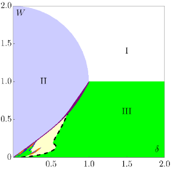
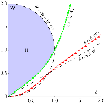
Recent research points out that two atomic clocks Rabi coupled to the same optical cavity mode synchronize and radiate with a common frequency Holland_Two_Ensemble_Theory ; Holland_Two_Ensemble_Theory_Followup ; Holland_Two_Ensemble_Expt ; Shammah . This is an analog of the weak lasing phenomenon and is reminiscent of the original synchronization experiment performed by C. Huygens in the 18th century. He studied the long-time dynamics of the pendulums of two clocks suspended from a common support and observed that after some time their phases and frequencies synchronize Pikovsky . In this paper, we map out the nonequilibrium phase diagram of two atomic ensembles in a bad cavity, see Fig. 1. In addition to monochromatic superradiance, we discover a plethora of fascinating dynamical behaviors – periodic, quasiperiodic and chaotic modulations of superradiance amplitude. Here we focus on monochromatic and periodic regimes, leaving more complicated behaviors for later Patra_2 ; Patra_3 . An interesting feature of the periodically modulated superradiance, where the power spectra are frequency combs (see Fig. 5), is that it makes the frequency of the ultrastable superradiant laser tunable.

(a) (a)

(b) (b)

Figure 2: Schematics of the setup (a) and energy level diagram (b). Two atomic ensembles A and B couple with Rabi coupling $\Omega$ (double-headed block arrows) to a heavily damped cavity mode (dashed line). Cavity intensity decays with a rate $\kappa$. The atoms (shown with solid arrows) in the two ensembles are effective two-level systems with level splittings $\omega_{A}$ and $\omega_{B}$. The dot-dashed line in (b) shows their shared ground state. The atoms are pumped incoherently from the ground state to their excited states via a third metastable state at a rate $W$.

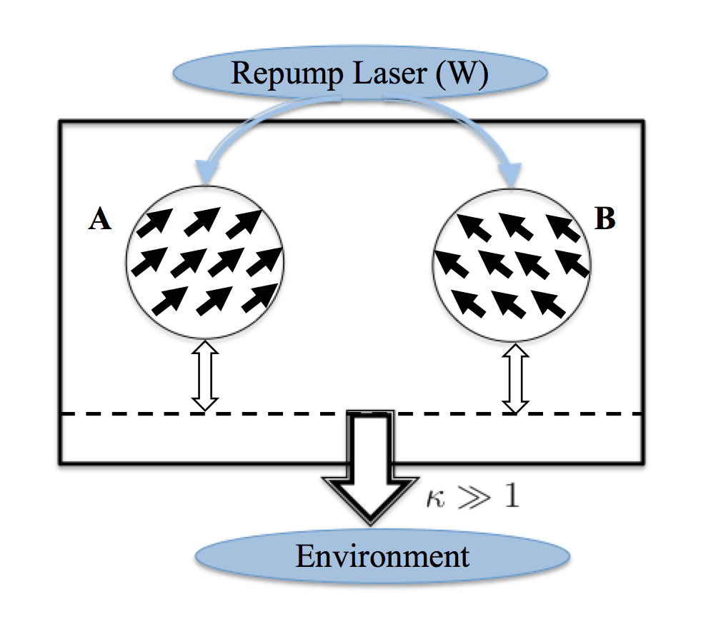
In the reminder of this section we describe our setup and summarize main results. We model the two atomic ensembles $(\tau=A,B)$ coupled to each other through a bad cavity mode, in the presence of dissipation and pumping (see Fig. 2), by the following master equation for the density matrix $\rho$:

$$\begin{split}\dot{\rho}=-\imath\big{[}\hat{H},\rho\big{]}+\kappa\mathcal{L}[a]\rho+W\sum_{\tau=A,B}\sum_{j=1}^{N}\mathcal{L}[\hat{\sigma}^{\tau}_{j+}]\rho,\\ \hat{H}=\omega_{0}\hat{a}^{\dagger}\hat{a}+\!\!\!\sum_{\tau=A,B}\big{[}\omega_{\tau}\hat{S}_{z}^{\tau}+\frac{\Omega}{2}\big{(}\hat{a}^{\dagger}\hat{S}_{-}^{\tau}+\hat{a}\hat{S}_{+}^{\tau}\big{)}\big{]},\end{split}$$ (1)

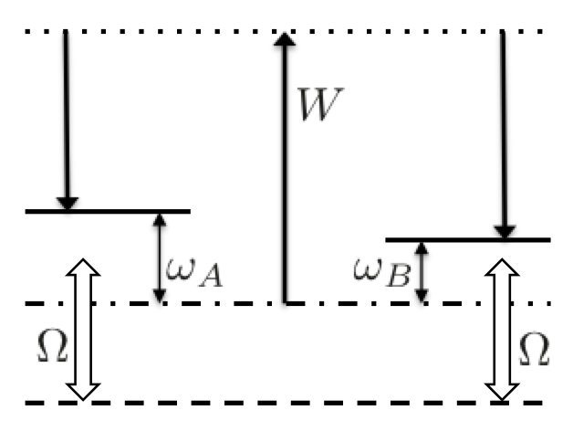
where the Hamiltonian for the system without energy nonconserving processes is $\hat{H}$ and the creation (annihilation) operator for the cavity mode $\omega_{0}$ is $\hat{a}^{\dagger}(\hat{a})$. Each ensemble contains $N(\approx 10^{6})$ atoms of the same type (e.g., $\prescript{87}{}{\textrm{Sr}}$ or $\prescript{87}{}{\textrm{Rb}}$). We regard the atoms as two-level systems and only focus on the two atomic energy levels most strongly coupled to the cavity mode. As a result, it is sufficient to represent the two ensembles with two collective spin operators

$$\hat{S}^{A,B}_{z}=\frac{1}{2}\sum_{j=1}^{N}\hat{\sigma}^{A,B}_{jz},\quad\hat{S}^{A,B}_{\pm}=\sum_{j=1}^{N}\hat{\sigma}^{A,B}_{j\pm},$$ (2)

where the Pauli operators $\hat{\bm{\sigma}}_{j}$ stand for individual atoms. Level spacings $\omega_{A}$ and $\omega_{B}$ of the two-level atoms in ensembles A and B, respectively, are controlled by separate Raman dressing lasers Holland_Two_Ensemble_Expt .

Besides the atom-cavity coherent coupling, we consider two energy nonconserving processes: (1) decay of the cavity mode with a rate $\kappa$ and (2) incoherent pumping of the atoms with a transverse laser at an effective repump rate $W$. We model these processes via Lindblad superoperators acting on the density matrix

$$\mathcal{L}[\hat{O}]\rho=\frac{1}{2}\big{(}2\hat{O}\rho\hat{O}^{\dagger}-\hat{O}^{\dagger}\hat{O}\rho-\rho\hat{O}^{\dagger}\hat{O}\big{)}.$$ (3)

In the bad cavity regime $\kappa\gg 1$, we neglect other sources of dissipation, such as spontaneous emission and background dephasing.

Our final goal is to analyze the light emitted by the cavity. To this end, we eliminate the cavity mode using the adiabatic approximation, which is exact in the $\kappa\rightarrow\infty$ limit, and then derive the following mean-field equations of motion in Sect. II.1 that describe the dynamics of the system in terms of two classical spins $\bm{s}^{A}$ and $\bm{s}^{B}$:

$$\dot{s}^{\tau}_{\pm} = \biggl{(}\pm\imath\omega_{\tau}-\frac{W}{2}\biggr{)}s^{\tau}_{\pm}+\frac{1}{2}s^{\tau}_{z}l_{\pm},$$ (4a)

$$\dot{s}^{\tau}_{z} = W\big{(}1-s^{\tau}_{z}\big{)}-\frac{1}{4}s^{\tau}_{+}l_{-}-\frac{1}{4}s^{\tau}_{-}l_{+},$$ (4b)

where

$$s^{\tau}_{\pm}=s_{x}^{\tau}\pm\imath s_{y}^{\tau}=\frac{2}{N}\langle\hat{S}_{\pm}^{\tau}\rangle,\quad s^{\tau}_{z}=\frac{2}{N}\langle\hat{S}_{z}^{\tau}\rangle,$$ (5)

are components of the classical spins and

$$\bm{l}=\sum_{\tau}\bm{s}^{\tau}=\bm{s}^{A}+\bm{s}^{B},$$ (6)

is the total classical spin. In the coordinate frame rotating with the angular frequency $\frac{1}{2}\sum_{\tau}\omega_{\tau}$ around the $z$-axis, the level spacings are

$$\omega_{A}=-\omega_{B}=\frac{\delta}{2},\quad\delta=\omega_{A}-\omega_{B},$$ (7)

where $\delta$ is the “detuning” between the two level-spacings. We note that Eq. (4) is valid for an arbitrary number $n$ of spatially separated ensembles of $N$ atoms each, identically coupled to the cavity. In Sect. II.2, we further derive the Fokker-Planck equation governing quantum fluctuations over the mean-field dynamics for $n$ ensembles. In the equations of motion and from now on we set the units of time and energy so that

$$N\Gamma_{c}=1,$$ (8)

where $\Gamma_{c}=\Omega^{2}/\kappa$ is the collective decay rate. Thus, the mean-field dynamics and nonequilibrium phase diagram for two atomic ensembles depend on only two dimensionless parameters $\delta$ and $W$. In a typical experiment $N\Gamma_{c}$ is approximately $1$ kHz, whereas $\delta$ and $W$ can be varied between zero and $4\pi$ MHz  Holland_One_Ensemble_Theory_1 ; Holland_One_Ensemble_Expt_1 ; Holland_One_Ensemble_Expt_2 ; Holland_Two_Ensemble_Expt .

Equations of motion (4) are axially symmetric, i.e., they are invariant with respect to $\bm{s}^{\tau}\to\mathbb{R}(\phi)\cdot\bm{s}^{\tau}$, where $\mathbb{R}(\phi)$ is a rotation by $\phi$ about the $z$-axis,

$$\mathbb{R}(\phi):(s^{\tau}_{\pm},s^{\tau}_{z})\longrightarrow(s^{\tau}_{\pm}e^{\pm\imath\phi},s^{\tau}_{z}).$$ (9)

Using axial symmetry and introducing a set of new variables,

$$s^{\tau}_{\pm}=s^{\tau}_{\perp}e^{\pm\imath\phi_{\tau}},\quad\phi_{A}=\Phi+\varphi,\quad\phi_{B}=\Phi-\varphi,$$ (10)

where $\varphi$ is defined modulo $\pi$, we factor out the evolution of the overall phase $\Phi$ from Eq. (4),

$$\dot{\Phi}=\frac{1}{2}\big{(}\omega_{A}+\omega_{B}\big{)}+\frac{\sin{2\varphi}}{4}\bigg{(}\frac{s^{A}_{z}s^{B}_{\perp}}{s^{A}_{\perp}}-\frac{s^{B}_{z}s^{A}_{\perp}}{s^{B}_{\perp}}\bigg{)}.$$ (11)

Note, $\dot{\Phi}$ as well as the equations of motion for the remaining five variables,

$$\begin{split}\dot{s}^{A}_{\perp}=-\frac{W}{2}s^{A}_{\perp}+\frac{s^{A}_{z}}{2}\big{(}s^{A}_{\perp}+s^{B}_{\perp}\cos{2\varphi}\big{)},\\ \dot{s}^{B}_{\perp}=-\frac{W}{2}s^{B}_{\perp}+\frac{s^{B}_{z}}{2}\big{(}s^{A}_{\perp}\cos{2\varphi}+s^{B}_{\perp}\big{)},\\ \dot{s}^{A}_{z}=W\big{(}1-s^{A}_{z}\big{)}-\frac{s^{A}_{\perp}}{2}\big{(}s^{A}_{\perp}+s^{B}_{\perp}\cos{2\varphi}\big{)},\\ \dot{s}^{B}_{z}=W\big{(}1-s^{B}_{z}\big{)}-\frac{s^{B}_{\perp}}{2}\big{(}s^{A}_{\perp}\cos{2\varphi}+s^{B}_{\perp}\big{)},\\ \dot{\varphi}=\frac{1}{2}\big{(}\omega_{A}-\omega_{B}\big{)}-\frac{\sin{2\varphi}}{4}\bigg{(}\frac{s^{A}_{z}s^{B}_{\perp}}{s^{A}_{\perp}}+\frac{s^{B}_{z}s^{A}_{\perp}}{s^{B}_{\perp}}\bigg{)},\end{split}$$ (12)

do not contain $\Phi$ as a consequence of the axial symmetry. This ensures that the values of $s^{\tau}_{\perp},s_{z}^{\tau}$ and $\varphi$ at subsequent times do not depend on the initial value of $\Phi$.

For two ensembles, Eq. (4) and Eq. (12) also possess a $\mathbb{Z}_{2}$ symmetry. Eq. (4) remains unchanged upon the replacement $\bm{s}^{\tau}\to\mathbb{\Sigma}\circ\mathbb{R}(\phi_{0})\cdot\bm{s}^{\tau}$, i.e., a rotation of the spins by a fixed angle $\phi_{0}$ about the $z$-axis, followed by an interchange of the two atomic clocks with a simultaneous change of the sign of the $y$-component

$$\mathbb{\Sigma}:\big{(}s_{\pm}^{A},s_{z}^{A},s_{\pm}^{B},s_{z}^{B}\big{)}\longrightarrow\big{(}s_{\mp}^{B},s_{z}^{B},s_{\mp}^{A},s_{z}^{A}\big{)}.$$ (13)

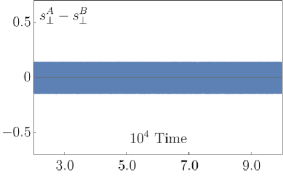
$\mathbb{Z}_{2}$-symmetric asymptotic solutions (attractors) obey $\bm{s}^{\tau}=\mathbb{\Sigma}\circ\mathbb{R}(\phi_{0})\cdot\bm{s}^{\tau}$, where $\phi_{0}$ depends on the initial condition. This condition defines a confining 4D submanifold of the full 6D phase space defined (independently of the initial conditions) by the following two constraints:

$$\begin{split}s_{\perp}^{A}=s_{\perp}^{B},\quad s_{z}^{A}=s_{z}^{B}.\end{split}$$ (14)

In a reference frame rotated by $\phi_{0}$ around the $z$-axis, the $\mathbb{Z}_{2}$-symmetric solutions satisfy

$$s^{A}_{x}=s^{B}_{x},\quad s^{A}_{y}=-s^{B}_{y},\quad s^{A}_{z}=s^{B}_{z}.$$ (15)

These three constraints define an invariant 3D submanifold, which is obtained by considering a fixed value of $\phi_{0}$ along with Eq. (14). An initial condition on this submanifold restricts the future dynamics on the same. The geometric meaning of the $\mathbb{Z}_{2}$ transformation is a reflection of the spin configuration through the plane containing the total spin $\bm{l}$ and the $z$-axis. In Eq. (12) it amounts to an interchange of $s_{\perp}^{A}$ with $s_{\perp}^{B}$ and of $s_{z}^{A}$ with $s_{z}^{B}$. In Eq. (11), one additionally needs to replace $\Phi\to-\Phi$ and set $\omega_{A}+\omega_{B}=0$.

For $\mathbb{Z}_{2}$-symmetric attractors, Eq. (15) implies that in a suitable coordinate frame $l_{x}=2s^{A}_{x}$, $l_{y}=0$, and Eq. (4) yields closed equations of motion for $\bm{s}^{A}$,

$$\dot{s}_{x} = -\frac{\delta}{2}s_{y}-\frac{W}{2}s_{x}+s_{z}s_{x},$$ (16a)

$$\dot{s}_{y} = \frac{\delta}{2}s_{x}-\frac{W}{2}s_{y},$$ (16b)

$$\dot{s}_{z} = W\big{(}1-s_{z}\big{)}-\big{(}s_{x}\big{)}^{2},$$ (16c)

where we dropped the superscript. Therefore, for a $\mathbb{Z}_{2}$ symmetric attractor it is sufficient to study Eq. (16). Even though Eq. (16) describes a motion of one spin, it is much more complex than Eq. (4) for a single atomic ensemble. Indeed, as we show in Appendix A, the phase diagram for the latter case is effectively 1D and contains only two phases (monochromatic superradiance and the normal phase).

Mean-field dynamics of several ensembles in a bad cavity have two types of fixed points, which we derive by equating the time derivatives to zero in Eq. (4). The first one is

$$s^{\tau}_{\pm}=0,\quad s^{\tau}_{z}=1.$$ (17)

This is a normal state, where atomic clocks are not synchronized and no light emanates from the cavity $(\langle\hat{a}^{\dagger}\hat{a}\rangle\propto|l_{-}|^{2}=0)$. In this phase (region I in Fig. 1), the atoms are maximally pumped $(s^{\tau}_{z}=1)$ and the cavity mode is not populated. We call this fixed point the trivial steady state (TSS). It is the only attractor with both the axial and $\mathbb{Z}_{2}$ symmetry.

The second type (non-trivial steady state or NTSS) corresponds to monochromatic superradiance (region II of Fig. 1). Here the damping is nontrivially balanced by the external pumping leading to a macroscopic population of the cavity mode. For two ensembles the NTSS reads

$$s^{A}_{-} =e^{-\imath(\Phi+\varphi)}\frac{l_{\perp}}{2}\sqrt{1+\frac{\delta^{2}}{W^{2}}},$$ (18)

$$s^{B}_{-} =e^{-\imath(\Phi-\varphi)}\frac{l_{\perp}}{2}\sqrt{1+\frac{\delta^{2}}{W^{2}}},$$

$$s^{A}_{z} =s^{B}_{z}=\frac{\delta^{2}+W^{2}}{2W},$$

where

$$l_{\perp}=\sqrt{2\big{(}1-(W-1)^{2}-\delta^{2}\big{)}},\quad\varphi=\arctan{\frac{\delta}{W}},$$ (19)

and $\Phi$ is an arbitrary angle. The NTSS comes to pass when the TSS loses stability on the quarter-circular arc depicting the boundary of Phases I and II. It spontaneously breaks the axial symmetry, while retaining the $\mathbb{Z}_{2}$ symmetry. Specifically, it is invariant under $\mathbb{\Sigma}\circ\mathbb{R}(-\Phi)$, where $\Phi$ is the overall phase in Eq. (18). NTSS is not a single point, but a one-parameter ($\Phi$) family of fixed points related to each other by rotations around the $z$-axis. Eqs. (7), (11) and (18) imply $\dot{\Phi}=0$. When $\omega_{A}+\omega_{B}\neq 0$, the axial symmetry of the NTSS is restored, and it becomes a trivial limit cycle with $\dot{\Phi}\neq 0$. Note also that for Eq. (12) the NTSS is a single fixed point, since $s_{\perp}^{A}$ and $s_{\perp}^{B}$ are independent of $\Phi$, while for Eq. (16) it reduces to two fixed points corresponding to $\Phi=0$ and $\pi$ in Eq. (18).

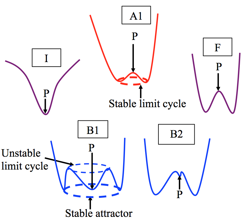
We determine the regions of stability of the TSS and NTSS in Sect. III.1. In Sect. III.2, we go beyond linear stability analysis (introducing the Poincaré-Birkhoff normal form) to explain the coexistence of NTSS with other attractors. We find that, in addition to the I-II boundary, TSS losses stability via a supercritical Hopf bifurcation (see Fig. 3) on the $\delta\geq 1$ part of the $W=1$ line separating Phases I and III in Fig. 1. After the bifurcation it gives rise to an infinitesimal limit cycle (frequency comb) as shown in Fig. 7. The NTSS, on the other hand, loses stability via a subcritical Hopf bifurcation (see Fig. 3 and Fig. 8), bringing about an unstable limit cycle before the bifurcation Intro_bifurc ; Kuznetsov ; Hilborn . This limit cycle is the separatrix – the boundary separating the basin of attraction of the NTSS from that of another attractor. As one nears criticality, the size of the separatrix shrinks, and after the bifurcation it disappears altogether. Therefore, any perturbation will push the dynamics far away from the fixed points right after the bifurcation, making it a catastrophic bifurcation. This not only explains the absence of any infinitesimal limit cycle after the bifurcation, but also justifies the coexistence (in the purple region of Fig. 1) of the NTSS with other attractors before the bifurcation. As explained in Fig. 3, the loss of stability of the NTSS is analogous to the first (rather than second Holland_Two_Ensemble_Theory ) order phase transition.

Figure 3: Cartoon demonstrating the similarity between Hopf bifurcations and phase transitions. Supercritical (subcritical) Hopf bifurcations are analogous to second (first) order phase transitions. The curves indicate 2D free energy plots and the direction of the flow towards stable attractors in the case of phase transitions and driven-dissipative dynamics, respectively. The leftmost curve depicts a stable equilibrium point P at the minimum. In a supercritical Hopf bifurcation (I $\rightarrow$ A1 $\rightarrow$ F) the fixed point loses stability by giving rise to a stable limit cycle. At the bifurcation the limit cycle is infinitesimally small just like the order parameter in a second order phase transition. In a subcritical Hopf bifurcation (I$\rightarrow$ B1 $\rightarrow$ B2 $\rightarrow$ F) an unstable limit cycle comes to exist before the bifurcation. This limit cycle acts as a separatrix between the basins of attraction of the fixed point P and another stable attractor.

Figure 4: $\mathbb{Z}_{2}$-symmetric limit cycles from the green parts of region III in Fig. 1 resemble potato chips. Here $(\delta,W)=(1.5,0.5)$. We only show spin $\bm{s}^{A}$ (blue arrow) representing the dynamics of atomic ensemble A, since spin $\bm{s}^{B}$ is related to $\bm{s}^{A}$ by the $\mathbb{Z}_{2}$ symmetry. In this regime the cavity radiates a frequency comb similar to the one shown in Fig. 5a. Individual spin trajectories for $\mathbb{Z}_{2}$-symmetry-broken limit cycles are similarly potato chip-like shaped, but the two spins are no longer tied to each other in a simple way.

For the sake of completeness, let us mention that in the absence of pumping (on the $\delta$ axis, sans the origin), the system goes to a nonradiative fixed point distinct from the TSS. For $W=0$, the mean-field equations of motion (4) reduce to a variant of the Landau-Lifshitz-Gilbert equation. The asymptotic solution only retains the axial symmetry, where both spins point along the negative $z$-axis. Finally, at the origin ($\delta=W=0$), the equations of motion are integrable. The attractor is a nonradiative fixed point that breaks both symmetries. We include a detailed discussion of these fixed points in Appendix C.

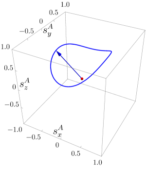
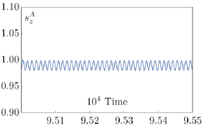
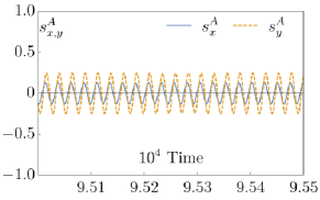
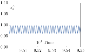
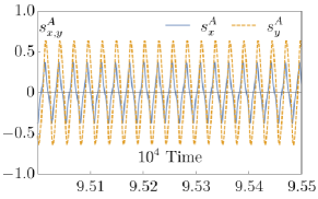
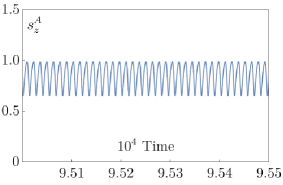
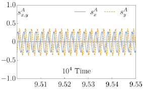
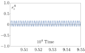
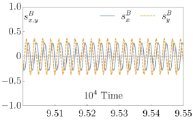
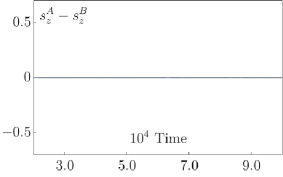
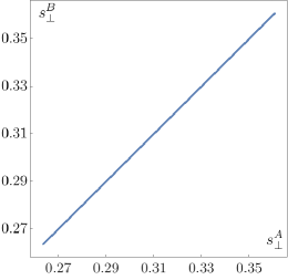
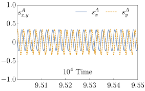
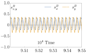
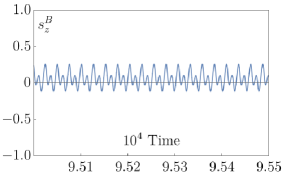
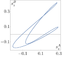
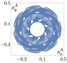
In region III of Fig. 1, all stable asymptotic solutions of Eq. (12) are time-dependent. In particular, there are limit cycles that lead to periodically modulated superradiance or frequency combs. None of them retain the axial symmetry. The limit cycle in the green part of region III possesses $\mathbb{Z}_{2}$ symmetry, while the ones in the light yellow subregion break it. A typical $\mathbb{Z}_{2}$-symmetric limit cycle is shown in Fig. 4. Using Eq. (16), we are able to analytically determine this limit cycle in various limits in Sect. IV.1.1. For example, when either $W\ll\delta$ or $1-W\ll 1$ (but $\delta$ is not too close to 1), in a suitably rotated frame,

$$s^{A}_{x} =s^{B}_{x}\approx \sqrt{2W(1-W)}\cos{(\omega t-\alpha)},$$ (20a)

$$s^{A}_{y} =-s^{B}_{y}\approx \sqrt{2W(1-W)}\sin{(\omega t)},$$ (20b)

$$s^{A}_{z} =s^{B}_{z}\approx W,$$ (20c)

where

$$\omega=\frac{1}{2}\sqrt{\delta^{2}-W^{2}},\qquad\tan{\alpha}=\frac{W}{2\omega}.$$ (21)

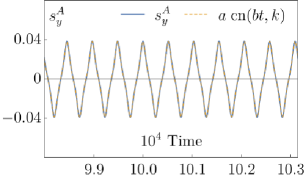
Then, the potato chip in Fig. 4 is flat and normal to the $z$-axis. For a comparison of Eq. (20) with the numerical result, see Fig. 12. We also note that the $z$-component of the limit cycle in the $\delta\gg W$ limit agrees with the result obtained with the help of quantum regression theorem in Ref. Holland_Two_Ensemble_Theory, . Especially interesting is the case when both $W$ and $\delta$ are close to 1, i.e., the vicinity of the tricritical point in Fig. 1. In this case, the harmonic approximation (20) breaks down and the solution for the limit cycle is now in terms of the Jacobi elliptic function cn, see Sect. IV.1.2.

We analyze the stability of $\mathbb{Z}_{2}$-symmetric limit cycles with the help of the Floquet technique in Sect. IV.2 and find that it becomes unstable as we cross the dotted line in Fig. 1. As a result, two new, symmetry-broken limit cycles related to each other by the $\mathbb{Z}_{2}$ symmetry operation emerge, see Sect. IV.3.

(a) (a)

(b) (b)

(c) (c)

Figure 5: Power spectra of periodically modulated superradiance in a rotating frame with the monochromatic superradiance frequency set as the origin. The unit of frequency $(f)$ is the collective decay rate $N\Gamma_{c}$. Top to bottom, $\mathbb{Z}_{2}$-symmetric limit cycle ($\delta=0.50$, $W=0.0802$) and two $\mathbb{Z}_{2}$-symmetry-broken limit cycles [($\delta,W)=(0.49,0.0802)$ and $(\delta,W)=(0.225,0.05)$]. Both in (a) and (b) the fundamental frequency is $f_{0}\approx 0.044$. Unlike (a), where only odd harmonics are present, in (b) even harmonics appear (most prominently at zero). In spite of both not having the $\mathbb{Z}_{2}$-symmetry, (c) visibly breaks the reflection symmetry about the vertical axis and features an overall frequency shift unlike (b).

Limit cycles in region III of the phase diagram are periodic solutions of Eq. (12) for given $W$ and $\delta=(\omega_{A}-\omega)/2$. They are closed curves in the 5D space with coordinates $s_{\perp}^{\tau}$, $s_{z}^{\tau}$, and $\varphi$ (mod $\pi$). Eq. (11) may introduce the second fundamental frequency $\omega_{q}$ depending on the reference frame and the limit cycle. Indeed, this equation implies

$$\Phi(t)=\Theta t+F(t),\quad\Theta=\frac{1}{2}(\omega_{A}+\omega_{B})+\omega_{q},$$ (22)

where $F(t)$ is periodic with the same period as the limit cycle and $\omega_{q}$ is the zeroth harmonic term in the Fourier series of the second term on the right hand side of Eq. (11). When $\Theta\neq 0$, the limit cycle precesses with constant angular frequency $\Theta$ in the full 6D space of components of $\bm{s}^{A}$ and $\bm{s}^{B}$, i.e., the corresponding attractor of Eq. (4) is an axially symmetric 2-torus. If $\Theta=0$, then $\Phi=\mathrm{const}$ and instead of a 2-torus we have a one parameter ($\Phi$) family of limit cycles related to each other via an overall rotation. Each of them breaks the axial symmetry. Regardless of the value of $\Theta$, we refer to all above attractors as a limit cycle at a point $(\delta,W)$ throughout this paper, keeping in mind that it is always a single limit cycle for Eq. (12). We are using a rotating frame such that $\omega_{A}+\omega_{B}=0$. In addition, $\omega_{q}=0$ for $\mathbb{Z}_{2}$-symmetric limit cycles, since the second term on the right hand side of Eq. (11) vanishes by $\mathbb{Z}_{2}$ symmetry. Therefore, $\Theta=0$ in this case.

Each of the above nonequilibrium phases of two atomic ensembles coupled to a heavily damped cavity mode has its unique signature in the power spectrum of the light radiated by the cavity. Experimentally, one measures the autocorrelation function of the radiated complex electric field. The power spectrum is the Fourier transform of this function, i.e., the modulus squared of the Fourier transform of the electric field. In terms of the classical spin variables, we identify the power spectrum to be proportional to $|l_{-}(f)|^{2}$ within mean-field approximation, where

$$l_{-}(f)=\int_{-\infty}^{+\infty}dt\;l_{-}(t)\;e^{2\pi\imath ft},\quad l_{-}=\sum_{\tau}s_{-}^{\tau}.$$ (23)

We derive this relationship between $l_{-}$ and the power spectrum in Appendix D starting from the master equation.

The power spectrum of monochromatic superradiance (NTSS) consists of a single peak at $f_{\mathrm{mc}}=(\omega_{A}+\omega_{B})/4\pi$, see Sect. V.1. For example, for $\prescript{87}{}{\textrm{Sr}}$ in a bad cavity, the peak appears approximately at $4.3\times 10^{5}$ GHz 3P0-1S0_87Sr . Subsequently, we show all spectra in a rotating frame and set the above superradiant frequency to be the origin.

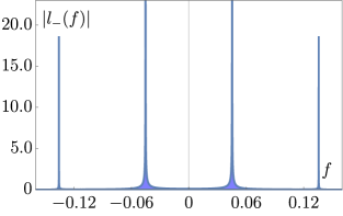
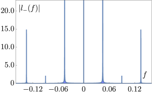
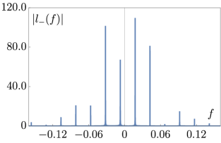
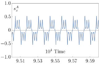
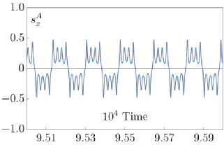
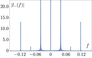
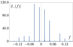
For the $\mathbb{Z}_{2}$-symmetric limit cycle the power spectrum is a frequency comb that contains only odd harmonics (see Fig. 5a). Moreover, because of the $\mathbb{Z}_{2}$ symmetry the spectrum possesses a reflection symmetry about the vertical axis. As one moves into the yellow subregion (to the left of the dashed line in Fig. 1), the $\mathbb{Z}_{2}$ symmetry breaks spontaneously. The power spectra of these limit cycles display both odd and even harmonics (see Fig. 5b). In particular, unlike the spectrum of the $\mathbb{Z}_{2}$-symmetric limit cycle, they have a pronounced peak at the origin. Despite the loss of the $\mathbb{Z}_{2}$ symmetry, the breaking of the reflection symmetry about the vertical axis is not so pronounced here. It is however possible to find examples of symmetry-broken limit cycles, where the reflection symmetry is visibly broken as in Fig. 5c. Another interesting feature of the spectrum in Fig. 5c is an overall shift of all frequencies by $\omega_{q}/2\pi$, see the discussion around Eq. (22). In Sect. V.2, we show more examples of power spectra (frequency combs) for different limit cycles.

Frequency combs arising from these limit cycles provide a range of frequencies (harmonics) around the main peak – the carrier frequency corresponding to the monochromatic superradiance. We will see that the spacing between consecutive peaks varies continuously in region III of the phase diagram and can take arbitrary values depending on $\delta$ and $W$. When $\delta$ and $W$ are of order 1, this spacing is many orders of magnitude smaller (tens of Hertz for $\prescript{87}{}{\textrm{Sr}}$) than the carrier frequency. For the ultrastable superradiant laser mentioned above this implies that its frequency is in principle tunable to within this amount.

II Semiclassical Dynamics and Quantum Corrections

In this paper we primarily explore the semiclassical dynamics of the system depicted in Eq. (1), see also Fig. 2. As mentioned above Eq. (4), one obtains the necessary evolution equations after adiabatically eliminating the cavity mode and employing the mean-field approximation $\langle\hat{O}_{1}\hat{O}_{2}\rangle\approx\langle\hat{O}_{1}\rangle\langle\hat{O}_{2}\rangle$. To derive the Fokker-Planck equation governing quantum fluctuations, we use the system size expansion (expansion in $N^{-\frac{1}{2}}$) Carmichael_1 ; Carmichael_2 ; Carmichael_3 . This also confirms the veracity of the mean-field equations as we obtain the same equations from the system size expansion.

II.1 Mean-Field Equations

We write the mean-field equations in terms of classical spins $\bm{s}^{\tau}$ introduced in Eq. (5), where the average of an operator $\hat{O}$ is $\mathrm{Tr}\,[\hat{O}\rho]$. To obtain the evolution equations for these variables, we first adiabatically eliminate the cavity mode Bad_cavity and then apply the mean-field approximation to the expression

$$\dot{\bm{s}}^{\tau}=\frac{2}{N}\mathrm{Tr}\,\big{[}\hat{\bm{S}}^{\tau}\dot{\rho}\big{]}=\frac{2}{N}\mathrm{Tr}\,\big{[}\hat{\bm{S}}^{\tau}\dot{\rho}_{\mathrm{at}}\big{]},$$ (24)

where $\rho_{\mathrm{at}}=\mathrm{Tr}\,_{\!F}(\rho)$ (traced over the cavity mode) is the atomic density matrix.

We start by rewriting the master equation (1) in the interaction representation,

$$\begin{split}\dot{\rho}_{I}=-\imath\big{[}\hat{H}_{I},\rho_{I}\big{]}+\kappa\mathcal{L}[a]\rho_{I}+W\sum_{\tau,j}\mathcal{L}[\hat{\sigma}^{\tau}_{j+}]\rho_{I},\\ \hat{H}_{I}=\frac{\delta}{2}\big{(}\hat{S}_{z}^{A}-\hat{S}_{z}^{B}\big{)}+\frac{\Omega}{2}\big{(}\hat{a}^{\dagger}\hat{J}_{-}+\hat{a}\hat{J}_{+}^{+}\big{)}.\end{split}$$ (25)

Here

$$\rho_{I} =e^{\imath(\hat{H}_{\mathrm{at}}+\hat{H}_{F})t}\rho e^{-\imath(\hat{H}_{\mathrm{at}}+\hat{H}_{F})t},$$ (26)

$$\hat{H}_{\mathrm{at}} =\frac{(\omega_{A}+\omega_{B})}{2}\big{(}\hat{S}_{z}^{A}+\hat{S}_{z}^{B}\big{)},\quad\hat{H}_{F}=\omega_{0}a^{\dagger}a$$

$$\hat{J}_{\pm} =\hat{S}^{A}_{\pm}+\hat{S}^{A}_{\pm}.$$

Next, we trace out the cavity mode in the above master equation and write the right hand side as a power series in $\Omega^{2}N/\kappa^{2}$. In the bad cavity regime ($\kappa\gg\Omega\sqrt{N}$), retaining only the zeroth order term and neglecting any memory effects, we derive

$$\begin{split}\dot{\rho}_{\mathrm{at}}=-\imath\big{[}\hat{h},\rho_{\mathrm{at}}\big{]}+\Gamma_{c}\mathcal{L}[\hat{J}_{-}]\rho_{\mathrm{at}}+W\sum_{\tau,j}^{N}\mathcal{L}[\hat{\sigma}^{\tau}_{j+}]\rho_{\mathrm{at}},\\ \hat{h}=\frac{\delta}{2}\big{(}\hat{S}_{z}^{A}-\hat{S}_{z}^{B}\big{)},\\ \end{split}$$ (27)

where we introduced the collective decay rate

$$\Gamma_{c}=\frac{\Omega^{2}}{\kappa}.$$ (28)

This procedure is exact in the limit $\kappa\to\infty$.

A heuristic explanation of the adiabatic approximation is as follows. In the interaction representation, the classical equation of motion for the cavity mode is

$$\frac{d\langle\hat{a}(t)\rangle}{dt}=-\frac{1}{2}\big{(}\kappa\langle\hat{a}(t)\rangle+\imath\Omega\langle\hat{J}_{-}(t)\rangle\big{)},$$ (29)

In the bad cavity regime, the cavity mode decays very quickly. As a result, the time derivative on the left hand side of Eq. (29) is negligible and we obtain

$$\langle\hat{a}\rangle\approx-\frac{\imath\Omega}{\kappa}\langle\hat{J}_{-}\rangle=-\frac{2\imath\Omega}{N\kappa}l_{-}.$$ (30)

If we extend this equality to the operator level and replace $\hat{a}$ with $\frac{\imath\Omega}{\kappa}\hat{J}_{-}$ in Eq. (1), we immediately arrive at Eq. (27). From Eq. (30) it is also apparent why, within the mean-field approach the intensity of emitted light ($\langle\hat{a}^{\dagger}\hat{a}\rangle$) is proportional to $|l_{-}|^{2}$.

Finally, using Eqs. (24), (27), and with the help of the mean-field approximation, we derive Eq. (4). In terms of the $x$, $y$ and $z$ components Eq. (4) reads

$$\dot{s}^{\tau}_{x} = -\omega_{\tau}s^{\tau}_{y}-\frac{W}{2}s^{\tau}_{x}+\frac{1}{2}s^{\tau}_{z}l_{x},$$ (31a)

$$\dot{s}^{\tau}_{y} = \omega_{\tau}s^{\tau}_{x}-\frac{W}{2}s^{\tau}_{y}+\frac{1}{2}s^{\tau}_{z}l_{y},$$ (31b)

$$\dot{s}^{\tau}_{z} = W\big{(}1-s^{\tau}_{z}\big{)}-\frac{1}{2}s^{\tau}_{x}l_{x}-\frac{1}{2}s^{\tau}_{y}l_{y}.$$ (31c)

Note also that our choice of units (8) of time and energy implies that $\Gamma_{c}$ scales as $N^{-1}$ with the number of atoms $N$. This ensures that the pumping and decay terms in Eq. (27) are comparable in magnitude. Moreover, in Sect. II.2 we show that assuming $\Gamma_{c}\propto N^{-1}$ helps achieve proper scaling factors in front of the semiclassical and the Fokker-Planck terms in the system size expansion.

II.2 Fokker-Planck Equation

In this subsection, we derive the Fokker-Planck equations for quantum fluctuations for $n$ atomic ensembles inside a bad cavity. The master equation is Eq. (27), but with

$$\hat{h}=\sum_{\tau=1}^{n}\omega_{\tau}\hat{S}_{z}^{\tau},$$ (32)

where $\omega_{\tau}$ are arbitrary. In the process, we also rederive the mean-field equations (31). We summarize the main steps and final results, referring the reader to a similar derivation in Refs. Carmichael_1, ; Carmichael_3, for further details.

Define the characteristic function $\chi$,

$$\chi\big{(}\bm{\xi},\bm{\xi^{*}},\bm{\eta},t\big{)}=\mathrm{Tr}\,\left[\prod_{\tau}\rho_{\mathrm{at}}e^{\imath\xi^{*}_{\tau}\hat{S}_{+}^{\tau}}e^{\imath\eta_{\tau}\hat{S}_{z}^{\tau}}e^{\imath\xi_{\tau}\hat{S}_{-}^{\tau}}\right].$$ (33)

Taking the time derivative of $\chi$ and using Eq. (27), we obtain, after some algebra, a partial differential equation for $\chi$. Then, we trade $\chi$ for the Glauber-Sudarshan $\cal P$-distribution function Glauber ; Sudarshan , which is the Fourier transform of $\chi$. In other words, we substitute

$$\chi=\int d^{2}\bm{v}\int d\bm{m}{\cal P}\big{(}\bm{v},\bm{v^{*}},\bm{m},t\big{)}e^{\imath\bm{\xi^{*}}\cdot\bm{v^{*}}}e^{\imath\bm{\xi}\cdot\bm{v}}e^{\imath\bm{\eta}\cdot\bm{m}}\!,$$ (34)

into the partial differential equation for $\chi$. This allows us to make the following replacements:

$$\partial_{\xi_{\tau}} \rightarrow\imath v_{\tau}, \partial_{\xi^{*}_{\tau}} \rightarrow\imath v^{*}_{\tau}, \partial_{\eta_{\tau}} \rightarrow\imath m_{\tau}$$ (35)

$$\xi_{\tau} \rightarrow-\imath\partial_{v_{\tau}}, \xi^{*}_{\tau} \rightarrow-\imath\partial_{v^{*}_{\tau}}, e^{\pm\imath\eta_{\tau}} \rightarrow e^{\pm\partial_{m_{\tau}}}.$$

After some additional manipulations (integration by parts to shift the differential operators onto ${\cal P}$), we arrive at a partial differential equation for the distribution function ${\cal P}\big{(}\bm{v},\bm{v^{*}},\bm{m},t\big{)}$ known as the Krammers-Moyal expansion,

$$\frac{\partial{\cal P}}{\partial t}=\bigg{(}\sum_{\tau}\mathbb{L}_{\tau}\bigg{)}{\cal P},$$ (36)

where

$$\mathbb{L}_{\tau}=\imath\omega_{\tau}\partial_{v_{\tau}}v_{\tau}+\frac{\Gamma_{c}}{2}\mathbb{A}_{\tau}\sum_{\tau^{\prime}}v_{\tau^{\prime}}+\\ +\frac{W}{2}\bigg{[}\frac{N}{2}\big{(}e^{\partial_{m_{\tau}}}\mathbb{B}^{2}_{\tau}-1\big{)}+\mathbb{C}_{\tau}m_{\tau}+\\ +\partial_{v_{\tau}}\big{(}2\mathbb{B}_{\tau}-1\big{)}v_{\tau}\bigg{]}+\textrm{c.c},$$ (37)

$$\mathbb{A}_{\tau} =v_{\tau}^{*}-e^{-\partial_{m_{\tau}}}v^{*}_{\tau}+2\partial_{v_{\tau}}m_{\tau}-\partial^{2}_{v_{\tau}}v_{\tau},$$ (38)

$$\mathbb{B}_{\tau} =e^{-\partial_{m_{\tau}}}+\partial_{v_{\tau}}\partial_{v^{*}_{\tau}},$$

$$\mathbb{C}_{\tau} =1-e^{-\partial_{m_{\tau}}}+\partial^{2}_{v_{\tau}}\partial^{2}_{v^{*}_{\tau}},$$

and ‘c.c’ stands for complex conjugate. The complex conjugate of $\partial_{z}$ is $\big{(}\partial_{z}\big{)}^{*}\equiv\partial_{z^{*}}$. The right-hand side of Eq. (36) contains derivatives of all orders.

To separate out the classical motion from the quantum fluctuations, we partition variables $\big{(}\bm{v},\bm{v^{*}},\bm{m}\big{)}$ as

$$v_{\tau}=N\left(\frac{s^{\tau}_{-}}{2}+N^{-\frac{1}{2}}\nu_{\tau}\right),$$ (39)

$$v_{\tau}^{*}=N\left(\frac{s^{\tau}_{+}}{2}+N^{-\frac{1}{2}}\nu_{\tau}^{*}\right),$$

$$m_{\tau}=N\left(\frac{s^{\tau}_{z}}{2}+N^{-\frac{1}{2}}\mu_{\tau}\right),$$

where $s^{\tau}_{\pm,z}$ are the classical spins defined in Eq. (5), and $\big{(}\bm{\nu},\bm{\nu^{*}},\bm{\mu}\big{)}$ correspond to quantum fluctuations over the classical motion. Let $\bar{{\cal P}}\big{(}\bm{\nu},\bm{\nu^{*}},\bm{\mu},t\big{)}$ be the probability density function of these fluctuations. By definition

$$\int d^{2}\bm{v}\int d\bm{m}{\cal P}\big{(}\bm{v},\bm{v^{*}},\bm{m},t\big{)}=\\ =\int d^{2}\bm{\nu}\int d\bm{\mu}\bar{{\cal P}}\big{(}\bm{\nu},\bm{\nu^{*}},\bm{\mu},t\big{)}\equiv 1.$$ (40)

Using Eqs. (39) and (40), we conclude

$$\bar{{\cal P}}\big{(}\bm{\nu},\bm{\nu^{*}},\bm{\mu},t\big{)}=N^{3n/2}{\cal P}\big{(}\bm{v},\bm{v^{*}},\bm{m},t\big{)}.$$ (41)

Substituting Eqs. (39) and (41) into Eq. (36) and recalling that $N\Gamma_{c}=1$, we obtain an expansion in powers of $N^{-\frac{1}{2}}$

$$\frac{\partial}{\partial t}\bar{{\cal P}}\big{(}\bm{\nu},\bm{\nu},\bm{\mu},t\big{)}=N^{\frac{1}{2}}\big{(}\textrm{semiclassical part}\big{)}+\\ +N^{0}\big{(}\textrm{Fokker-Planck equation}\big{)}+\mathcal{O}\left(N^{-\frac{1}{2}}\right),$$ (42)

where the semi-classical part is

$$\sum_{\tau}\bigg{[}\big{(}\#\big{)}\partial_{\nu_{\tau}}+\big{(}\#\big{)}\partial_{\nu^{*}_{\tau}}+\big{(}\#\big{)}\partial_{\mu_{\tau}}\bigg{]}\bar{{\cal P}}$$ (43)

We note that the coefficient at $N^{\frac{1}{2}}$ contains only the first order derivatives with respect to $\nu_{\tau}$, $\nu^{*}_{\tau}$ and $\mu_{\tau}$; the one at $N^{0}$ – the first and second order derivatives with respect to the same variables; etc. In $N\rightarrow\infty$ limit, the semiclassical part needs to vanish. Moreover, the coefficients at each partial derivative in Eq. (43) must vanish separately, because otherwise we would end up with a time-independent constraint on the probability density function $\bar{\cal P}$ of quantum fluctuations. The resulting three conditions are precisely the mean-field equations of motion (4).

Finally, neglecting terms of the order $N^{-\frac{1}{2}}$ in Eq. (42), we obtain the Fokker-Planck equation

$$\frac{\partial\bar{\cal P}}{\partial t}=\bigg{(}\sum_{\tau}\mathbb{L}^{(2)}_{\tau}\bigg{)}\bar{\cal P},$$ (44)

where

$$\mathbb{L}^{(2)}_{\tau}=\bigg{[}\imath\omega_{\tau}+\frac{1}{2}\big{(}W-s_{z}^{\tau}\big{)}\bigg{]}\partial_{\nu_{\tau}}\nu_{\tau}+\frac{1}{2}\partial_{\mu_{\tau}}\mu_{\tau}+\\ +\frac{1}{4}s_{-}^{\tau}l_{-}\partial^{2}_{\nu_{\tau}}+\frac{1}{64}\big{[}2W(1-2s_{z}^{\tau})+s_{-}^{\tau}l_{+}\big{]}\partial^{2}_{\mu_{\tau}}+\\ +\frac{W}{2}\partial_{\nu_{\tau}}\partial_{\nu^{*}_{\tau}}+\frac{W}{4}s_{-}^{\tau}\partial_{\nu_{\tau}}\partial_{\mu_{\tau}}+\textrm{c.c}.$$ (45)

This operator does not contain derivatives of orders higher than the second.

III Stability Analysis of TSS and NTSS

In this section, we determine regions of stability for the TSS (normal nonradiative phase) and NTSS (monochromatic superradiance). These fixed points are described by Eqs. (17) and (18), respectively. We show that linear stability analysis of the reduced spin equations (16) obtains the same regions of stability as that of full equations of motion (4). This means that perturbations that respect the $\mathbb{Z}_{2}$-symmetry destabilize these steady states before or at the same time as the ones that do not. Then, going beyond the linear analysis, we establish that the TSS and NTSS undergo different types of Hopf bifurcations.

III.1 Linear Stability Analysis of the Fixed Points

III.1.1 Jacobian Matrix

To analyze the stability of a fixed point $({\bm{s}}^{A}_{0},{\bm{s}}^{B}_{0})$ we linearize the right hand side of Eq. (31) about $({\bm{s}}^{A}_{0},{\bm{s}}^{B}_{0})$. This produces a $6\times 6$ Jacobian matrix,

$$\mathbb{J}=\begin{bmatrix}[1.5]\mathbb{D}^{A}&\mathbb{X}^{A}\\ \mathbb{X}^{B}&\mathbb{D}^{B}\end{bmatrix},$$ (46)

where

$$\mathbb{D}^{\tau} =\begin{bmatrix}[1.5]\frac{1}{2}\big{(}s^{\tau}_{z0}-W\big{)}&-\omega_{\tau}&\frac{1}{2}l_{x0}\\ \omega_{\tau}&\frac{1}{2}\big{(}s^{\tau}_{z0}-W\big{)}&\frac{1}{2}l_{y0}\\ -\frac{1}{2}\big{(}l_{x0}+s^{\tau}_{x0}\big{)}&-\frac{1}{2}\big{(}l_{y0}+s^{\tau}_{y0}\big{)}&-W\end{bmatrix},$$ (47)

$$\mathbb{X}^{\tau} =\begin{bmatrix}[1.5]\frac{1}{2}s^{\tau}_{z0}&0&0\\ 0&\frac{1}{2}s^{\tau}_{z0}&0\\ -\frac{1}{2}s^{\tau}_{x0}&-\frac{1}{2}s^{\tau}_{y0}&0\end{bmatrix}.$$

Its eigenvalues are the characteristic values of the fixed point $({\bm{s}}^{A}_{0},{\bm{s}}^{B}_{0})$, while the eigenvectors are the corresponding characteristic directions. If a characteristic value has a positive real part at certain point $(\delta,W)$, the fixed point is unstable. Accordingly, we define the region of stability of a fixed point as the region in the $\delta-W$ plane, where all characteristic values have negative real parts.

III.1.2 Stability of TSS

We observe that the TSS exists everywhere on the $\delta-W$ plane. Substituting $({\bm{s}}^{A}_{0},{\bm{s}}^{B}_{0})$ from Eq. (17) into Eq. (46), we determine the characteristic equation as

$$\big{[}Q_{3}(\lambda)\big{]}^{2}\equiv\bigg{[}\big{(}W+\lambda\big{)}\times\\ \times\bigg{(}\lambda^{2}+\big{(}W-1\big{)}\lambda+\frac{1}{4}\big{(}W^{2}+\delta^{2}-2W\big{)}\bigg{)}\bigg{]}^{2}=0.$$ (48)

The roots of the above equation,

$$\begin{split}\lambda_{1,2}=-W,\\ \lambda_{3,4}=\frac{1}{2}\big{[}\big{(}1-W\big{)}+\sqrt{1-\delta^{2}}\big{]},\\ \lambda_{5,6}=\frac{1}{2}\big{[}\big{(}1-W\big{)}-\sqrt{1-\delta^{2}}\big{]},\end{split}$$ (49)

are the characteristic values of the TSS. All eigenvalues are double degenerate. The symmetry responsible for the degeneracy is the $\mathbb{Z}_{2}$ transformation (13), i.e., $\mathbb{J}\mathbb{\Sigma}-\mathbb{\Sigma}\mathbb{J}=0$ for the TSS, where $\mathbb{\Sigma}$ is the $6\times 6$ matrix representation of the mapping (13). This implies that if $|\lambda\rangle$ is a characteristic direction with the characteristic value $\lambda$, so is $\mathbb{\Sigma}|\lambda\rangle$.

For $\delta>1$ the characteristic values $\lambda_{3,4}$ and $\lambda_{5,6}$ are complex and conjugate to each other. Their real part changes sign from negative to positive as $W$ goes from $1^{+}$ to $1^{-}$. This pair of degenerate characteristic values simultaneously crosses the imaginary axis at $W=1$, i.e., a Hopf bifurcation takes place across the $W=1,\delta\geq 1$ half-line. In Sect. III.2, we will see that this Hopf bifurcation is supercritical giving rise to a stable limit cycle as illustrated in Fig. 3. We will find in Sect. III.2 below that the the real and imaginary parts of characteristic values $\lambda_{3,4}$ and $\lambda_{5,6}$ determine the amplitude ($\propto\sqrt{1-W}$) and the period ($\approx 4\pi/\sqrt{\delta^{2}-1}$) of the limit cycle, respectively, at its inception. The analytical expression (20) for this $\mathbb{Z}_{2}$-symmetric limit cycle in various limits further corroborates these results.

Note also that when $\omega_{A}+\omega_{B}\neq 0$ this limit cycle rotates around the $z$-axis with a constant angular frequency $\frac{\omega_{A}+\omega_{B}}{2}$ according to Eq. (11) [the additional term on the right hand side vanishes by $\mathbb{Z}_{2}$ symmetry]. It thus becomes a 2D torus and the bifurcation is fixed point $\to$ torus, rather than fixed point $\to$ limit cycle Resonant_Hopf . This marks an important difference between this bifurcation and the TSS $\to$ NTSS transition, which is fixed point $\to$ limit cycle for any $\omega_{A}+\omega_{B}\neq 0$.

For $\delta<1$ all roots are real. For these values of $\delta$, $\lambda_{3,4}<0$ only when

$$(W-1)^{2}+\delta^{2}>1.$$ (50)

The above condition also ensures that $\lambda_{5,6}<0.$ The quarter arc arising from this condition that separates Phases I and II in Fig. 1 depicts a supercritical Hopf bifurcation. Indeed, in a rotating frame where $\omega_{A}+\omega_{B}\neq 0$, NTSS is a trivial limit cycle and the roots $\lambda_{3}$ and $\lambda_{4}$ acquire imaginary parts $\pm\frac{\imath(\omega_{A}+\omega_{B})}{2}$ and cross the imaginary axis in unison. Outside the quarter arc, TSS is a node, i.e., all characteristic values are negative. Inside it turns into a saddle point – a few characteristic values become positive. At the same time a stable NTSS comes into existence. On the bifurcation line the NTSS is indistinguishable from the TSS, but deviates from it significantly as we move deeper into Phase II. Later in this section we provide an alternative interpretation of the TSS $\to$ NTSS transition as a supercritical pitchfork bifurcation using the reduced spin equations (16).

III.1.3 Stability of NTSS

From Eq. (18), we observe that for the NTSS to exist, $l_{\perp}$ needs to be real. So, it only exists inside the semicircle $\delta^{2}+(W-1)^{2}=1$. However, presently we show that it is not stable everywhere inside this semicircle. As we have done for the TSS earlier, we derive the characteristic equation for the NTSS,

$$\lambda P_{2}(\lambda)P_{3}(\lambda)=0,$$ (51)

where the polynomials $P_{2}$ and $P_{3}$ are

$$P_{2}(\lambda) \equiv \lambda^{2}+c_{2}\lambda+c_{1},$$ (52a)

$$P_{3}(\lambda) \equiv \lambda^{3}+c_{2}\lambda^{2}+c_{1}\lambda+c_{0},$$ (52b)

with the coefficients

$$c_{0} =W\bigg{(}W-\frac{W^{2}+\delta^{2}}{2}\bigg{)},$$ (53)

$$c_{1} =2W-\frac{W^{2}+3\delta^{2}}{2},$$

$$c_{2} =\frac{3W^{2}-\delta^{2}}{2W}.$$

We observe that one characteristic value is always zero. This corresponds to the characteristic direction along the overall rotation around the $z$-axis [changing $\Phi$ in Eq. (18)]. Recall that NTSS is a collection of fixed points on a circle. Thus, when we perturb one such point along this direction, it neither goes to infinity nor does it come back to the original point. Instead, it just lands onto the neighboring NTSS point.

Figure 6: The domain of stability of the NTSS (Phase II) is shown in blue. NTSS exists inside the semicircle (dashed line) $\delta^{2}+(W-1)^{2}=1$. The dot-dashed line is $\delta=\sqrt{3}W$ [Eq. (54b)]. Red triangles and green squares denote the lines $\delta=\delta_{+}(W)$ and $\delta=\delta_{-}(W)$, respectively, where $\delta_{\pm}(W)$ are defined in Eq. (55). This picture shows that the minimal description of Phase II is $\big{[}\delta^{2}+(W-1)^{2}<1\big{]}\wedge\big{[}\delta<\delta_{-}(W)\big{]}$. Since the $\delta=\delta_{-}(W)$ line is inside the semicircle, the NTSS loses stability via a Hopf bifurcation (see the text).

We use the Routh-Hurwitz stability criterion Gradshteyn_Ryzhik to determine the boundary between Phases II and III. According to this criterion, the NTSS is stable when $\big{(}c_{i}>0\;\textrm{for all $i$}\big{)}\wedge\big{(}c_{2}c_{1}>c_{0}\big{)}$. Moreover, $\big{(}c_{2}c_{1}>c_{0}\big{)}\wedge\big{(}c_{2}>0\big{)}\wedge\big{(}c_{0}>0\big{)}$ guarantees $\big{(}c_{1}>0\big{)}$. Therefore, the NTSS is stable if and only if

$$(W-1)^{2}+\delta^{2} < 1,$$ (54a)

$$W > \frac{\delta}{\sqrt{3}},$$ (54b)

$$3\delta^{4}-\big{(}6W^{2}+4W\big{)}\delta^{2}+W^{3}\big{(}8-W\big{)} > 0,$$ (54c)

where the last inequality corresponds to $c_{2}c_{1}>c_{0}$. Its left hand side is a biquadratic polynomial in $\delta$. We write it as $\big{[}\delta^{2}-\delta_{+}^{2}(W)\big{]}\big{[}\delta^{2}-\delta_{-}^{2}(W)\big{]}$, where

$$\delta_{\pm}^{2}(W)=\frac{2W}{3}\bigg{(}\frac{3W}{2}+1\pm\sqrt{3W^{2}-3W+1}\bigg{)},$$ (55)

$$\delta_{+}(W)>\delta_{-}(W)>0,\textrm{ (for $\delta,W>0$).}$$

Taking into account $\delta>0$ and $W>0$, we see that Eq. (54c) requires

$$\big{[}\delta>\delta_{+}(W)\big{]}\vee\big{[}\delta<\delta_{-}(W)\big{]}.$$ (56)

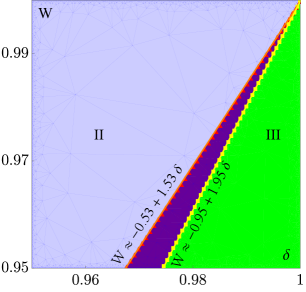
Plotting the above two conditions along with Eqs. (54a) and (54b) in Fig. 6, we conclude that the equation for the lower ($W<1$) part of the Phase II boundary is

$$\delta=\delta_{-}(W).$$ (57)

This means that the real part of at least one of the roots of $P_{3}(\lambda)$ changes sign from negative to positive as we cross the boundary. Since $P_{3}(\lambda)=0$ is a cubic equation with real coefficients, this implies one of the following two complimentary circumstances:

1. A real root is equal to zero at criticality.

2. Near the boundary, the cubic polynomial has one real and two complex conjugate roots. None of them are zero on the boundary. The real part of the complex conjugate roots changes sign at criticality. This second scenario entails a Hopf bifurcation.

$P_{3}(\lambda)$ has a zero root only when $c_{0}=0$, i.e., on the semicircle $\delta^{2}+(W-1)^{2}=1$. We observe from Fig. 6 that the condition $c_{2}c_{1}>c_{0}$ is violated first, while $c_{i}>0$ for all $i$ still holds. This proves that the NTSS must obey the condition 2 above. In other words, it loses stability via a Hopf bifurcation. Moreover, in Sect. III.2 we prove that it, in fact, undergoes a subcritical Hopf bifurcation to bring about a coexistence region near the boundary between Phases II and III, see also Figs. 3 and 8.

III.1.4 Stability Analysis with Symmetric Spin Equations

Since the TSS and NTSS both have $\mathbb{Z}_{2}$ symmetry, we also carry out linear stability analysis with the reduced spin equations (16) to learn more about perturbations destabilizing these steady states. The fixed points of Eq. (16) are

$$s_{-}=0,\quad s_{z}=1,\quad$$ (58)

and

$$s_{-}=\pm\frac{l_{\perp}e^{-\imath\varphi}}{2}\sqrt{1+\frac{\delta^{2}}{W^{2}}},\quad s_{z}=\frac{\delta^{2}+W^{2}}{2W},$$ (59)

where $\varphi$ and $l_{\perp}$ are given in Eq. (19). Eq. (58) is the TSS (17), where we now only need the components of spin $\bm{s}^{A}$. Similarly, Eq. (59) is the NTSS (18), but now we also need to pick a specific frame where $l_{y}=0$ [see the text above Eq. (16)]. Note that with this choice of initial-condition-dependent frame, NTSS turns from a one parameter family of fixed points into two fixed points.

The linearization of Eq. (16) about a fixed point $\bm{s}=\bm{s}_{0}$ yields the Jacobian matrix

$$\mathbb{J}=\begin{bmatrix}[1.5]s_{z0}-\frac{1}{2}W&-\frac{1}{2}\delta&s_{x0}\\ \frac{1}{2}\delta&-\frac{1}{2}W&0\\ -2s_{x0}&0&-W\end{bmatrix}.$$ (60)

Substituting explicit solutions for the TSS and the NTSS, we obtain

$$\textrm{TSS}:\qquad Q_{3}(\lambda) =0,$$ (61a)

$$\textrm{NTSS}:\qquad P_{3}(\lambda) =0,$$ (61b)

where $Q_{3}(\lambda)$ and $P_{3}(\lambda)$ are defined in Eqs. (48) and (52b). We saw above that it was the behavior of the roots of $Q_{3}(\lambda)$ and $P_{3}(\lambda)$ that determined the regions of stability of the TSS and NTSS. Thus, linear stability analysis with both Eqs. (4) and (16) produces the same regions, but for different reasons. For the TSS, factoring out the $\mathbb{Z}_{2}$ symmetry from Eq. (4) reduces the degree of the degeneracy for each of the three distinct characteristic values from two to one. On the other hand, for the NTSS the deviations destabilizing the fixed point are $\mathbb{Z}_{2}$-symmetric. Therefore, for our problem it is sufficient to analyze the reduced spin equations (16) to study the properties of the TSS and the NTSS near criticality.

From the point of view of the reduced spin equation, the TSS $\to$ NTSS transition is what is known as a supercritical pitchfork bifurcation Intro_bifurc . This is a situation when there is a single stable fixed point before and three fixed points – one unstable and two stable – after the bifurcation. At criticality all these fixed points coincide.

III.2 Different Types of Hopf Bifurcations: Beyond Linear Stability

(a) (a)

(b) (b)

(c) (c)

(d) (d)

(e) (e)

(f) (f)

Figure 7: Evolution of the limit cycle born out of the supercritical Hopf bifurcation at $(\delta,W)=(1.1,1)$. We fix $\delta=1.1$ and gradually decrease $W$ moving vertically from Phase I (TSS) into the green part of region III ($\mathbb{Z}_{2}$-symmetric limit cycle) in Fig. 1. Top to bottom, $W=0.999,0.99$ and 0.98 in the first, second and third row. We plot $s^{A}_{x}$ and $s^{A}_{y}$ vs. time in the first column and $s^{A}_{z}$ vs. time in the second.

(a) (a)

(b) (b)

Figure 8: Limit cycle with finite amplitude right after subcritical Hopf bifurcation of the NTSS at $(\delta,W)=(0.888,0.800)$. Here $(\delta,W)=(0.890,0.800)$. We show $s^{A}_{x}$ and $s^{A}_{y}$ vs. time in (a) and $s^{A}_{z}$ vs. time in (b).

To differentiate between Hopf bifurcations, we need to go beyond the linear stability analysis Intro_bifurc ; Kuznetsov ; Hilborn . Since only two characteristic directions become unstable in a Hopf bifurcation, one can determine its essential features by projecting the dynamics onto a 2D manifold called the “center manifold”. At criticality, this manifold is the vector space spanned by the two unstable characteristic directions. The dynamics on the center manifold near criticality in terms of polar coordinates $(s,\theta)$ take the form

$$\dot{s} = s\bigg{(}\gamma+\sum_{j=1}^{\infty}a_{j}s^{2j}\bigg{)},$$ (62a)

$$\dot{\theta} = \omega+\sum_{j=1}^{\infty}b_{j}s^{2j},$$ (62b)

where the origin is at the fixed point and $\gamma\pm\imath\omega$ are the complex conjugate characteristic values responsible for the instability of the fixed point; $\gamma=0$ at criticality. Eq. (62) is a perturbative expansion near the fixed point. Its right hand side is known as the “Poincaré-Birkhoff normal form”. We derive Eq. (62) for the TSS and NTSS starting from Eq. (16), including the coefficient $a_{1}$ as a function of $\delta$ and $W,$ in Appendix B.

(a) (a)

(b) (b)

Figure 9: Plots of the coefficient $a_{1}$ in the Poincaré-Birkhoff normal form (62) near Hopf bifurcations of the TSS and NTSS. The bifurcation is supercritical (subcritical) if $a_{1}<0$ ($a_{1}>0$). (a) $a_{1}$ is negative for the TSS at $\delta=1.5$ for a substantial range of $W$ around $W=1$. It behaves in a similar manner elsewhere near the bifurcation along the $W=1,\delta\geq 1$ boundary of Phases I and III in Fig. 1. (b) Here $W=0.95$. The Hopf bifurcation of the NTSS takes place at $\delta_{H}(0.95)=0.97$, where $a_{1}=0.46$. Note the finite neighborhood around $\delta_{H}$ where $a_{1}$ is positive. The qualitative variation of $a_{1}$ for NTSS remains the same elsewhere near the bifurcation along the boundary of Phases II and III.

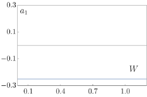
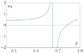
Suppose $\dot{s}=0$. Since $s$ is small near the bifurcation, Eq. (62a) yields $s\big{(}\gamma+a_{1}s^{2}\big{)}\approx 0$. There are two solution, $s=0$ and $s=s_{H}=\sqrt{-\gamma/a_{1}}$. In order to have a limit cycle we need $s_{H}$ to be real. Thus, if $a_{1}<0$, the limit cycle comes to exist only after $\gamma(\delta,W)$ becomes positive, i.e., after the bifurcation, signaling a supercritical Hopf bifurcation. Linearizing the right hand side of Eq. (62a) near $s_{H}$, we find $d\Delta s/dt=-2\gamma\Delta s$, where $\Delta s=s-s_{H}$. Since after the bifurcation $\gamma>0$, the limit cycle is stable in the supercritical scenario. Eq. (62b) shows that near the bifurcation the polar angle $\theta=\omega t$. Therefore, the period of the limit cycle is $2\pi/\omega$, where $\omega$ is evaluated at the criticality. On the other hand, if $a_{1}>0$, the limit cycle must exist before the bifurcation has taken place. This is because in order for $s_{H}$ to be real we need $\gamma<0$, which is the case only before the bifurcation. This type of bifurcation is known as a subcritical Hopf bifurcation. From the stability analysis we observe that this limit cycle is unstable. As a consequence, it serves as the separatrix of the basin of attraction for the fixed point, see Fig. 3.

We plot representative examples of $a_{1}$ across the Hopf bifurcation for the TSS and NTSS in Fig. 9 . For the TSS, $a_{1}<0$ near the half-line $W=1,\delta\geq 1$ corroborating our earlier claim that it loses stability via a supercritical Hopf bifurcation. Fig. 7 shows the (initially infinitesimal) limit cycle emerging right after the bifurcation of the TSS. In contrast, the NTSS undergoes a subcritical Hopf bifurcation on the boundary of Phases II and III. Indeed, there is a region in Fig. 9b around $\delta_{H}(W)$ – the value of $\delta$ on the boundary at a given $W$ – where $a_{1}>0$.

III.2.1 Coexistence Due to Subcritical Hopf Bifurcation

In accordance with the above discussion, the unstable limit cycle existing before the bifurcation separates basins of attraction of the NTSS and another attractor, which continues into Phase III after NTSS loses stability. An example of such an attractor is the limit cycle shown in Fig. 8. As we approach the bifurcation from inside Phase II, $\gamma$ tends to zero. Since the size of the separatrix (unstable limit cycle) is proportional to $\sqrt{|\gamma|}$, the basin of attraction of the NTSS shrinks to zero. Thus, there is a region of coexistence of NTSS with other attractors inside Phase II (shown in purple in Fig. 1). Its right boundary coincides with the Phase II-III boundary, while the left boundary is somewhere inside Phase II. In Sect. IV.1.3 we determine the shape of this region analytically in the vicinity of the tricritical point $\delta=W=1$.

Observe that the dashed line in Fig. 1 merges with the Phase II-III boundary at a certain point. Numerically, we find that the value of $W$ at this point is $W_{c}\approx 0.575$. For $W>W_{c}$, the attractor to the right of Phase II is the $\mathbb{Z}_{2}$-symmetric limit cycle. Therefore, NTSS coexists with this limit cycle in the purple sliver near the boundary for $W_{c}<W<1$. For $W<W_{c}$, it coexists with other time-dependent asymptotic solutions of Eq. (4), such as chaotic superradiance Patra_2 ; Patra_3 . We have also observed empirically that the coexistence region is an order of magnitude thinner in the latter case.

We determine the left boundary of the coexistence region in Fig. 1 using the following numerical method:

1. Determine the time-dependent asymptotic solution immediately to the right of $\delta_{H}(W)$ for a fixed $W$.

2. Record ten random $\big{(}{\bm{s}}^{A},{\bm{s}}^{B}\big{)}$ on this solution. We use these as initial conditions in the next step.

3. Decrease $\delta$ and see whether any of these initial conditions lead to a time-dependent asymptotic solution. If yes, repeat steps 2 and 3. If not, record the value of $\delta$ as $\delta_{\textrm{End}}(W)$. Check that for $0<\delta\leq\delta_{\textrm{End}}(W)$ the time evolution for all these initial conditions converges to the NTSS.

4. Repeat this procedure for other values of $W$.

Note that $a_{1}$ in Fig. 9b decreases to zero as we move horizontally into Phase II, i.e., decrease $\delta$ below $\delta_{H}(W)$ keeping $W$ fixed. A way to estimate the left boundary of the coexistence region is to obtain the value of $\delta=\delta_{a_{1}=0}(W)$ where $a_{1}$ becomes zero. However, we find that this estimate is rather inaccurate. Consider, for example, four distinct values of $W$ in Table 1. Two of them are greater than $W_{c}$ and the other two are smaller. For each $W$, we report the values of $\delta_{H}(W),\delta_{a_{1}=0}(W)$ and $\delta_{\textrm{End}}(W)$. In all these cases, an independent numerical analysis using the procedure outlined above reveals that the coexistence ends well before $\delta_{a_{1}=0}(W)$. This indicates that to accurately determine its left boundary, one needs to consider higher order terms in the Poincaré-Birkhoff normal form.

$W$	$\delta_{H}(W)$	$\delta_{a_{1}=0}(W)$	$\delta_{\textrm{End}}(W)$
0.30	0.410	0.358	0.408
0.45	0.592	0.520	0.588
0.65	0.782	0.687	0.759
0.95	0.974	0.820	0.967

Table 1: Comparison of $\delta_{H}(W),\delta_{a_{1}=0}(W)$ and $\delta_{\textrm{End}}(W)$. For all four values of $W$, $\delta_{\textrm{End}}(W)>\delta_{a_{1}=0}(W)$, i.e., the coexistence of NTSS with other attractors ends before a naive estimate based on the first two orders of the perturbative expansion (62).

IV Limit Cycles

In this section, we study limit cycles in region III of the nonequilibrium phase diagram in Fig. 1. We will see in Sect. V that these attractors translate into periodic modulations of the superradiance amplitude – the cavity radiates frequency combs in this regime. The radiation power spectrum has various features depending on the symmetry of the limit cycle, such as presence or absence of even harmonics of the limit cycle frequency, symmetry with respect to the vertical axis, and a shift of the carrier frequency.

In most of Phase III, we observe $\mathbb{Z}_{2}$-symmetric limit cycles, such as the ones in Figs. 4, 10, and 11. When $\delta$ is large or $W(1-W)$ is small, oscillations of spin components become harmonic and we determine the approximate form of the limit cycle analytically. A special situation arises in the vicinity of the tricritical point $(\delta,W)=(1,1)$ in Fig. 1. Now the oscillations are anharmonic, but we are still able to derive analytic expressions for the spins in terms of the Jacobi elliptic function cn. This also helps us determine the shape of the coexistence region of the NTSS with $\mathbb{Z}_{2}$-symmetric limit cycles near the tricritical point. Eventually, limit cycles lose the $\mathbb{Z}_{2}$-symmetry across the dashed line in Fig. 1. We determine this line and independently explain the mechanism of the symmetry breaking with the help of Floquet stability analysis. We conclude this section by discussing properties of limit cycles with broken $\mathbb{Z}_{2}$ symmetry, such as the ones in Figs. 16e, 17 and 18.

IV.1 Solution for the $\mathbb{Z}_{2}$-Symmetric Limit Cycle in Various Limits

As discussed below Eq. (22), a $\mathbb{Z}_{2}$-symmetric limit cycle at a given $(\delta,W)$ is in fact a one parameter family of limit cycles that differ from each other only by the constant value of the net phase $\Phi$. Eq. (10) shows that the projection $\bm{l}_{\perp}=(l_{x},l_{y})$ of the total spin onto the $xy$-plane moves on a line making a constant angle $\Phi$ with the $x$-axis. It is convenient to rotate the coordinate system, as we did in Eq. (16), so that $\bm{l}_{\perp}$ is along the $x$-axis. Eq. (15) then relates the components of $\bm{s}^{A}$ and $\bm{s}^{B}$ and we see that it is sufficient to study reduced spin equations (16) to describe $\mathbb{Z}_{2}$-symmetric limit cycles.

(a) (a)

(b) (b)

(c) (c)

(d) (d)

(e) (e)

(f) (f)

Figure 10: A $\mathbb{Z}_{2}$-symmetric limit cycle at $(\delta,W)=(0.44,0.056)$. Classical spins $\bm{s}^{A}$ and $\bm{s}^{B}$ describe the mean-field dynamics of two atomic ensembles in a bad cavity. Spin components fulfill $\mathbb{Z}_{2}$-symmetry conditions $s_{\perp}^{A}=s_{\perp}^{B}$ and $s_{z}^{A}=s_{z}^{B}$, see Eq. (14). For these values of the detuning $\delta$ between level spacings of the two ensembles and pumping $W,$ the cavity radiates the frequency comb shown in Fig. 20.

(a) (a)

(b) (b)

Figure 11: $s^{A}_{\perp}$ vs. $s^{B}_{\perp}$ and $s^{A}_{z}$ vs. $s^{B}_{z}$ projections of the $\mathbb{Z}_{2}$-symmetric limit cycle at $(\delta,W)=(0.44,0.056)$, same as in Fig. 10. These are straight lines passing through the origin with $45^{\circ}$ slope due to the $\mathbb{Z}_{2}$ symmetry of the attractor. Note the difference with the $\mathbb{Z}_{2}$-asymmetric limit cycle at a nearby point $(\delta,W)=(0.42,0.056)$ in Fig. 17.

(a) (a)

(b) (b)

(c) (c)

(d) (d)

Figure 12: Comparison between numerics and perturbative solutions (66) and (74) for the $\mathbb{Z}_{2}$ symmetric limit cycle. We show the $y$-components only, the agreement for other components is similarly good. (a) $\delta=5.0,W=10^{-3}.$ (b) $\delta=5.0,W=1-10^{-3}.$ (c) $\delta=500,W=0.5.$ (d) $\delta=1-(500/755)\times 10^{-3},W=1-10^{-3}.$ Note the highly anharmonic nature of the oscillations in (d).

IV.1.1 Harmonic Solution

Here we work out a simple solution for the $\mathbb{Z}_{2}$-symmetric limit cycle valid in various limits. Expressing $s_{x}$ through $s_{y}$ and $\dot{s}_{y}$ in Eq. (16b) and substituting the result into Eq. (16a), we find

$$\ddot{s}_{y}+\dot{s}_{y}\big{(}W-s_{z}\big{)}+s_{y}\bigg{(}\frac{\delta^{2}}{4}+\frac{W^{2}}{4}-\frac{W}{2}s_{z}\bigg{)}=0.$$ (63)

We interpret this as a damped harmonic oscillator with a complicated feedback. To cancel the damping term, we assume $s_{z}\approx W$. We will later check the self-consistency of this assumption. For a constant $s_{z}$, Eq. (63) is simple to solve and using additionally Eq. (16b), we derive

$$s_{y}=a\sin{\omega t},\qquad s_{x}=a\cos{(\omega t-\alpha)},$$ (64)

where

$$\omega=\frac{\sqrt{\delta^{2}-W^{2}}}{2},\quad\alpha=\arctan\frac{W}{2\omega}.$$ (65)

Substituting this $s_{x}$ into Eq. (16c), we notice that it has solutions of the form $s_{z}=C_{1}+C_{2}\cos{(2\omega t+\beta)}$, where we require $C_{1}=W$ for consistency. This requirement also fixes the constants $a$, $C_{2}$ and $\beta$, so that (recall that $0<W<1$ in Phase III)

$$s_{x} = \sqrt{2W(1-W)}\cos{(\omega t-\alpha)},$$ (66a)

$$s_{y} = \sqrt{2W(1-W)}\sin{\omega t},$$ (66b)

$$s_{z} = W-\frac{W}{\delta}(1-W)\sin{(2\omega t-\alpha)}.$$ (66c)

We see that the assumption $s_{z}\approx W$ is reasonable when $W(1-W)\ll\delta$. Substituting $s_{z}$ from Eq. (66c) into the coefficient of the $s_{y}$ term in Eq. (63), we obtain $(\delta^{2}-W^{2})/4+\left[W^{2}(1-W)/2\delta\right]\sin{(2\omega t-\alpha)}$. Therefore, to neglect the time-dependent part of $s_{z}$ in the frequency term in Eq. (63), we additionally need

$$\omega^{2}=\frac{\delta^{2}-W^{2}}{4}\gg\frac{W^{2}}{2\delta}(1-W).$$ (67)

These conditions are fulfilled when: (1) $\delta$ is large, (2) $W$ is small and $\delta$ is of order 1, and (3) $W$ is close to 1 and $\delta$ is not too close to $W$, namely, $\delta-W\gg 1-W$. In these regimes, Eq. (66) agrees with numerical results very well, see Fig. 12.

In particular, for small $W$ the solution takes the form

$$s_{x} \approx \sqrt{2W}\cos{(\delta t/2)},$$ (68a)

$$s_{y} \approx \sqrt{2W}\sin{(\delta t/2)},$$ (68b)

$$s_{z} \approx 0,$$ (68c)

while just below the Hopf bifurcation $W=1$ line,

$$s_{x} \approx \sqrt{2(1-W)}\cos{(\omega t-\alpha)},$$ (69a)

$$s_{y} \approx \sqrt{2(1-W)}\sin{\omega t},$$ (69b)

$$s_{z} \approx 1,$$ (69c)

where $\omega\approx\frac{1}{2}\sqrt{\delta^{2}-1}$. Note that the amplitude and frequency of the limit cycle in this limit matches those in Sect. III.1.2. Generally, if we neglect the small sine term in Eq. (66c), Eq. (66) describes an ellipse perpendicular to the $z$-axis. This is what becomes of the potato chip in Fig. 4 in the harmonic approximation. When $W\ll\delta$ the ellipse turns into a circle.

IV.1.2 Elliptic Solution Close to $W=\delta=1$ Point

The harmonic approximation breaks down in the vicinity of the $(\delta,W)=(1,1)$ point, where Phases I, II and III merge in Fig. 1. In this case the frequency $\omega$ of the limit cycle is small and inequality (67) does not hold. However, now we can exploit the fact that oscillations are slow. As a result, derivatives are suppressed by a factor of $\omega$ in Eq. (16), so that

$$s_{x} = \frac{W}{\delta}s_{y}+\frac{2}{\delta}\dot{s}_{y}\approx\frac{W}{\delta}s_{y},$$ (70a)

$$s_{z} = 1-\frac{s^{2}_{x}}{W}-\frac{\dot{s}_{z}}{W}\approx 1-\frac{s^{2}_{x}}{W}.$$ (70b)

Let

$$W=1-\epsilon,\quad\delta=1+r,$$ (71)

where $\epsilon>0$ and $r$ are small. Substituting $s_{z}$ from Eq. (70b) into Eq. (63), we obtain

$$\ddot{s}_{y}-\dot{s}_{y}\left(2s_{y}^{2}+\epsilon\right)+\frac{s_{y}}{2}\left(r+s_{y}^{2}\right)=0,$$ (72)

where we kept only the leading orders in $\epsilon$ and $r$ in the coefficients. Assuming $r$ is of the order of $\epsilon$, we see from Eq. (69) that in the harmonic solution $s_{y}$ and the frequency $\omega$ are both of the order $\sqrt{\epsilon}$. Then, the $\dot{s}_{y}$ term in Eq. (72) is negligible. We also verified that this as well as the approximations in Eq. (70) are self-consistent regardless of the magnitude of $|r|/\epsilon$ using the Jacobi elliptic solution for $s_{y}$ we work out below.

Neglecting the $\dot{s}_{y}$ term in Eq. (72) , we find

$$\ddot{s}_{y}+\frac{r}{2}s_{y}+\frac{1}{2}s^{3}_{y}=0.$$ (73)

This reduces to the standard equation for the Jacobi elliptic function cn Gradshteyn_Ryzhik ; Abramowitz_Stegun via a substitution

$$s_{y}(t)=a\;\textrm{cn}(bt,k),$$ (74)

where

$$b^{2}=\frac{r}{2(1-2k^{2})},\quad a^{2}=\frac{2k^{2}r}{1-2k^{2}}.$$ (75)

Eq. (75) provides two constraints for three undetermined parameters $a,b$ and $k$. We derive one more constraint by minimizing the effect of the the $\dot{s}_{y}$ term that we neglected in Eq. (72). Specifically, we multiply Eq. (72) by $\dot{s}_{y}$ and integrate over one period. Since the first and the last terms turn into complete derivatives, we are left with

$$\epsilon\langle\dot{s}^{2}_{y}\rangle=2\langle s^{2}_{y}\dot{s}^{2}_{y}\rangle.$$ (76)

Evaluating the integrals on both sides of this equation, we derive

$$a^{2}=\frac{\epsilon}{2}Y(k),$$ (77)

where

$$Y(k)=\frac{5k^{2}\big{[}(2k^{2}-1)E+(1-k^{2})K\big{]}}{2(k^{4}-k^{2}+1)E-(2-k^{2})(1-k^{2})K},$$ (78)

and $K\equiv K(k)$ and $E\equiv E(k)$ are complete elliptic integrals of the first and second kind, respectively. Matching Eq. (77) to $a^{2}$ in Eq. (75) yields an equation for $k$,

$$Z(k)\equiv\frac{4k^{2}}{5(1-2k^{2})Y(k)}=\frac{\epsilon}{r}.$$ (79)

This equation along with Eq. (75) specify all three constants of $s_{y}(t)$ in Eq. (74). A plot of $Z(k)$ for $r<0$ appears in Fig. 14. We see that when $\epsilon/r$ is between $-8/5$ and the maximum of $Z(k)$ at approximately $-1.50$, there are two solutions for $k$. Numerically we observe that the evolution with Eq. (16) picks up the solution with smaller $k$ in this case.

The oscillation period,

$$T=\frac{4K(k)\sqrt{2|1-2k^{2}|}}{\sqrt{|r|}},$$ (80)

diverges when $r\to 0$ at fixed $\epsilon/r$.

For small $r$ and $\epsilon$, the condition (67) of validity of the harmonic solution reads $r\gg\epsilon>0$. Hence, the elliptic and harmonic solutions must agree in the limit $\epsilon/r\to 0^{+}$, which we now check. The solution of (79) to the first order in $\epsilon/r$ is $k^{2}\approx\epsilon/r$. Elliptic functions become harmonic when $k\to 0$. In particular, $s_{y}=a\,\textrm{cn}(bt)\approx a\cos{(bt)}$ Elliptic . Further, Eq. (75) yields $a^{2}=2\epsilon$ and $b^{2}=r/2$, which agrees exactly with $a^{2}$ and $\omega^{2}$ for the harmonic solution for small $\epsilon$, $r$, and $\epsilon/r$. We also checked that this agreement does not go beyond the leading order in $\epsilon/r$.

IV.1.3 Gauging the Taper of Coexistence Region Near $W=\delta=1$

Figure 13: Linear fit to the boundaries of the coexistence region (purple) near $\delta=W=1$. The right boundary is the subcritical Hopf bifurcation line. Yellow squares is the numerical result for this line and solid yellow line with the slope $1.95$ is the best linear fit to these points. Orange triangles depict points on the left boundary of the coexistence region. The best linear fit to these points (solid orange line) has a slope 1.53.

Figure 14: The function $Z(k)$ defined in Eq. (79) in the domain $1/\sqrt{2}<k<1$. We show $Z(1)=-1.6$ by the dashed line. In this interval $Z(k)$ reaches its maximum of -1.50 at $k\approx 0.96$.

The coexistence region gradually tapers off to a point $(\delta,W)=(1,1)$, see Fig. 13. Let us determine the angle with which the coexistence region approaches its pinnacle. To that end, we utilize the elliptic solution for the $\mathbb{Z}_{2}$-symmetric limit cycle valid near $\delta=W=1$ point. The right boundary of the coexistence region is the subcritical Hopf bifurcation line (57). Linearizing Eq. (57) in $\epsilon$ and $r$, we find $\epsilon=-2r$. Therefore, the line tangential to the right boundary at $(\delta,W)=(1,1)$ has a slope

$$\tan{\theta_{R}}=2.$$ (81)

We also see that $r<0$ in the coexistence region, because $\epsilon=1-W>0$.

The left boundary of the coexistence region near $\delta=W=1$ point is the line where the elliptic solution (74) ceases to exist. Since $r<0$, in order for $b^{2}$ in Eq. (75) to be positive, we need $k>1/\sqrt{2}$. Thus, for the elliptic solution to exist inside the coexistence region, the solution of Eq. (79) must satisfy $1/\sqrt{2}<k<1$. We plot $Z(k)$ in this interval in Fig. 14. Observe that $Z(1)=-8/5=-1.6$ and the maximum value of $Z(k)$ is approximately $-1.50$. Therefore, Eq. (79) has no solutions in the desired range when $\epsilon\leq-1.50r$ and the slope of the tangent to the left boundary of the coexistence region at $(\delta,W)=(1,1)$ is

$$\tan{\theta_{L}}\approx 1.50.$$ (82)

Eqs. (81) and (82) agree well with the results of numerical analysis shown in Fig. 13. The taper angle of the coexistence region near $\delta=W=1$ is $\theta_{R}-\theta_{L}\approx\arctan{(2)}-\arctan{(1.5)}\approx 7^{\circ}$.

IV.2 Stability of the $\mathbb{Z}_{2}$-Symmetric Limit Cycle: Floquet Analysis

$(\delta,W)$	$\delta_{>},$ $\rho_{1}$, $\rho_{2}$, $\rho_{3}$	$\delta_{<},$ $\rho_{1}$, $\rho_{2}$, $\rho_{3}$
(0.40, 0.051)	0.42, 1.0, 0.99, 0.27	0.41, 1.0, 1.1, 0.24
(0.52, 0.10)	0.54, 1.0, 0.97, 0.14	0.53, 1.0, 1.0+, 0.066
(0.54, 0.15)	0.56, 1.0, 1.0-, 0.069	0.55, 1.0, 1.0+, 0.031
(0.53, 0.20)	0.53, 1.0, 0.99, 0.033	0.52, 1.0, 1.0+, 0.031
(0.55, 0.25)	0.55, 1.0, 1.0-, 0.017	0.54, 1.0, 1.0+, 0.016
(0.54, 0.30)	0.58, 1.0, 1.0-, 0.00+	0.57, 1.0, 1.0+, 0.00+
(0.60, 0.35)	0.61, 1.0, 1.0-, 0.00+	0.60, 1.0, 1.0+, 0.00+
(0.64, 0.40)	0.64, 1.0, 0.97, 0.00+	0.63, 1.0, 1.1, 0.00+
(0.64, 0.45)	0.67, 1.0, 0.90, 0.00+	0.66, 1.0, 1.0+, 0.00+
(0.67, 0.50)	0.69, 1.0, 0.93, 0.00+	0.68, 1.0, 1.1, 0.00+
(0.70, 0.55)	0.71, 1.0, 0.98, 0.00+	0.70, 1.0, 1.1, 0.00+

Table 2: As discussed in the text, we determine points $(\delta,W)$ where the $\mathbb{Z}_{2}$-symmetric limit cycle loses stability by requiring that $|s_{z}^{A}-s_{z}^{B}|$ exceeds a certain threshold at large times. The 1st column shows some of these points. Here we compare them to the results of Floquet stability analysis. The 2nd and 3rd columns show Floquet multipliers $\rho_{1}$, $\rho_{2}$, and $\rho_{3}$ for the same $W$ as in the 1st column and two values of $\delta$, $\delta=\delta_{>}$ and $\delta_{<}$. We see that one of $\rho_{i}$ exceeds 1, signaling instability, at approximately the same value of $\delta$ as in the 1st column. We indicate values in the intervals $(0.00,0.01)$, $(1.00,1.01)$ and $(0.99,1.00)$ as $0.00+$, $1.0+$ and $1.0-$.

In this section, we analyze the stability of $\mathbb{Z}_{2}$-symmetric limit cycles using the Floquet theory. As before, it is convenient to rotate the coordinate system by a fixed angle so that the $\mathbb{Z}_{2}$-symmetric limit cycle obeys the constraints (15). We introduce symmetric coordinates covering the $\mathbb{Z}_{2}$-symmetric submanifold,

$$s_{x}=\frac{s^{A}_{x}+s^{B}_{x}}{2},\quad s_{y}=\frac{s^{A}_{y}-s^{B}_{y}}{2},\quad s_{z}=\frac{s^{A}_{z}+s^{B}_{z}}{2},$$ (83)

and transverse coordinates that take the dynamics away from it,

$$q_{x}=s^{A}_{x}-s^{B}_{x},\quad q_{y}=s^{A}_{y}+s^{B}_{y},\quad q_{z}=s^{A}_{z}-s^{B}_{z}.$$ (84)

Recasting Eq. (31) in terms of the new variables, we have,

$$\dot{s}_{x} = -\frac{\delta}{2}s_{y}-\frac{W}{2}s_{x}+s_{z}s_{x},$$ (85a)

$$\dot{s}_{y} = \frac{\delta}{2}s_{x}-\frac{W}{2}s_{y}-\frac{1}{4}q_{y}q_{z},$$ (85b)

$$\dot{s}_{z} = W\big{(}1-s_{z}\big{)}-s_{x}^{2}-\frac{1}{4}q_{y}^{2}$$ (85c)

$$\dot{q}_{x} = -\frac{\delta}{2}q_{y}-\frac{W}{2}q_{x}+s_{x}q_{z},$$ (85d)

$$\dot{q}_{y} = \frac{\delta}{2}q_{x}+\left(s_{z}-\frac{W}{2}\right)q_{y},$$ (85e)

$$\dot{q}_{z} = -Wq_{z}-s_{x}q_{x}-s_{y}q_{y}.$$ (85f)

For the unperturbed $\mathbb{Z}_{2}$-symmetric limit cycle $q_{x}=q_{y}=q_{z}=0$ and $\bm{s}$ obeys the reduced spin equations (16). To analyze the linear stability with respect to symmetry-breaking perturbations, we linearize Eq. (85) in $\bm{m}$,

$$\dot{q}_{x} = -\frac{\delta}{2}q_{y}-\frac{W}{2}q_{x}+s_{x}(t)q_{z},$$ (86a)

$$\dot{q}_{y} = \frac{\delta}{2}q_{x}+\left(s_{z}(t)-\frac{W}{2}\right)q_{y},$$ (86b)

$$\dot{q}_{z} = -Wq_{z}-s_{x}(t)q_{x}-s_{y}(t)q_{y},$$ (86c)

where $s_{x}(t),s_{y}(t)$ and $s_{z}(t)$ are the spin components for the $\mathbb{Z}_{2}$-symmetric limit cycle, which we obtain separately by simulating Eq. (16). They play the role of periodic in time coefficients for the linear system (86).

By Floquet theorem the general solution of Eq. (86) is

$$\bm{q}(t)=\sum_{i=1}^{3}d_{i}e^{\varkappa_{i}t}\bm{p}_{i}(t),$$ (87)

where $\bm{p}_{i}(t)$ are linearly independent vectors periodic with the same period $T$ as the limit cycle, $d_{i}$ are arbitrary constants, and $\varkappa_{i}$ are the Floquet exponents.. To evaluate $\varkappa_{i}$, we first compute the monodromy matrix $\mathbb{M}=[\mathbb{S}(0)]^{-1}\mathbb{S}(T)$, where $\mathbb{S}(t)$ is a $3\times 3$ matrix whose columns are any three linearly independent solutions $\bm{q}_{i}(t)$ of Eq. (86). We determine $\bm{q}_{i}(t)$ by simulating Eq. (86) for one period for three randomly chosen initial conditions. The eigenvalues of the monodromy matrix $\rho_{i}=e^{\varkappa_{i}T}$ are known as characteristic multipliers. If one of the them is greater than one, the corresponding $\varkappa_{i}$ is positive and the $\mathbb{Z}_{2}$-symmetric limit cycle is unstable.

Figure 15: Absolute values of Floquet multipliers $|\rho_{i}|$ as functions of $\delta$ for the $\mathbb{Z}_{2}$-symmetric limit cycle at $W=0.40$. The red dotted line marks the point of symmetry breaking (loss of stability) according to the criterion $|s_{z}^{A}-s_{z}^{B}|>0.01$ at large times. Across criticality $|\rho_{1}|=1$ indicates the presence of nearby $\mathbb{Z}_{2}$-symmetric limit cycles related by overall rotations about the $z$-axis, whereas $|\rho_{3}|<1$ corresponds to a stable direction.

(a) (a)

(b) (b)

(c) (c)

(d) (d)

(e) (e)

(f) (f)

Figure 16: A limit cycle at $(\delta,W)=(0.42,0.056)$. Classical spins $\bm{s}^{A}$ and $\bm{s}^{B}$ describe the mean-field dynamics of two atomic ensembles A and B coupled to a heavily damped cavity mode. This limit cycle breaks the $\mathbb{Z}_{2}$-symmetry because $s_{\perp}^{A}-s_{\perp}^{B}$ and $s_{z}^{A}-s_{z}^{B}$ are nonzero and time-dependent (see also Fig. 17), unlike for the $\mathbb{Z}_{2}$-symmetric limit cycle at a nearby point $(\delta,W)=(0.44,0.056)$ shown in Fig. 10. For these values of the detuning $\delta$ between the two ensembles and pumping $W,$ the cavity radiates the frequency comb shown in Fig. 21.

    

(a) (a)

(b) (b)

Figure 17: $s^{A}_{\perp}$ vs. $s^{B}_{\perp}$ and $s^{A}_{z}$ vs. $s^{B}_{z}$ projections for the limit cycle in Fig. 16e. The difference with the $\mathbb{Z}_{2}$-symmetric limit cycle at a nearby point $(\delta,W)=(0.44,0.056)$ shown in Fig. 11 is dramatic. Nevertheless, both plots are symmetric with respect to reflection through the diagonal. Note also self-intersections that result from projecting a multi-dimensional (5D) curve onto 2D planes.

In our case, one of the characteristic multipliers is identically equal to one. This is because, as we discussed below Eq. (22), each limit cycle is a member of a one parameter family of limit cycles related to each other by rotations around the $z$-axis. An infinitesimal rotation of the original limit cycle produces an identical limit cycle just in a ‘wrong’ coordinate system, where $q_{x}$ and $q_{y}$ are infinitesimal but nonzero. This must be a periodic solution of Eq. (86). Specifically, $\Delta s_{x}^{\tau}=-\Delta\Phi s_{y}^{\tau}$ and $\Delta s_{y}^{\tau}=\Delta\Phi s_{x}^{\tau}$ for a rotation by $\Delta\Phi$. Eq. (84) then implies $q_{x}=-2\Delta\Phi s_{y}$ and $q_{y}=2\Delta\Phi s_{x}$. Therefore,

$$\bm{p}_{1}=\begin{pmatrix}s_{y}\\ -s_{x}\\ 0\end{pmatrix},$$ (88)

is a solution of Eq. (86) with the same period $T$. We verify this directly using also Eq. (16). Thus, Eq. (87) simplifies to

$$\bm{q}(t)=d_{1}\bm{p}_{1}(t)+d_{2}e^{\varkappa_{2}t}\bm{p}_{2}(t)+d_{3}e^{\varkappa_{3}t}\bm{p}_{3}(t).$$ (89)

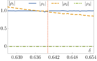
We observe that the $\mathbb{Z}_{2}$-symmetric limit cycle becomes unstable as we cross the dashed line in Fig. 1 and the asymptotic dynamics of the two ensembles loose the $\mathbb{Z}_{2}$ symmetry in the yellow region to its left. Near this line of symmetry breaking the other two characteristic multipliers ($\rho_{2}$ and $\rho_{3}$) are also real. Both are less than one to the immediate right of this line, while one of them becomes greater than one as we cross the line and enter the yellow subregion, see, e.g., Fig. 15.

In practice, we find it more convenient to determine the line of symmetry breaking by monitoring the asymptotic value of $|s_{z}^{A}-s_{z}^{B}|$, which is zero for a $\mathbb{Z}_{2}$-symmetric limit cycle. When this quantity exceeds a certain threshold (0.01 at $t>2\times 10^{4}$ in our algorithm), we declare the symmetry broken and the $\mathbb{Z}_{2}$-symmetric limit cycle unstable. This method agrees with our Floquet stability analysis to within few percent as evidenced by Table 2 and Fig. 15.

IV.3 Limit Cycles without $\mathbb{Z}_{2}$ symmetry

(a)   (a)

(b)   (b)

(c)           (c)

Figure 18: An asymmetric limit cycle at $(\delta,W)=(0.225,0.05)$ from the dark blue subregion near the origin of Fig. 1. This is a periodic attractor when we factor out the net phase $\Phi(t)$ as in Eq. (12). Otherwise, $\Phi(t)$ brings about another frequency $\omega_{q}$ transforming it into a 2-torus in the full phase-space. Plot (c) is the projection of this torus onto the $s_{x}^{A}-s_{y}^{A}$ plane. Given enough time the trajectory densely fills an annulus with radii $s^{A}_{\perp,\max}$ and $s^{A}_{\perp,\min}$. The additional frequency disappears if we move into a rotating frame or consider rotationally invariant quantities as in (a) and (b), but shows up as an overall shift by $\omega_{q}/2\pi$ in the power spectrum of the light radiated by the cavity, see Fig. 5c.

(a) (a)

(b) (b)

(d) (d)

Figure 19: Different limit cycles in the $\mathbb{Z}_{2}$-symmetric green island to the left of the symmetry breaking line in Fig. 1; $(\delta,W)=(0.23,0.0802)$ and $(0.12,0.055)$ in the first and second rows, respectively. In the main figures, we plot $s_{x}^{A}$ vs. time, whereas in the insets we corroborate the $\mathbb{Z}_{2}$-symmetry in the $s_{z}^{A}-s_{z}^{B}$ projections. The initial condition for the two limit cycles in the first column, which are unstable in the full 6D phase-space, is $(\bm{s}_{0}^{A},\bm{s}_{0}^{B})=(0.4,-0.469,0.7,0.4,0.469,0.7)$. The ones in the second column are stable in the full phase-space. The initial condition for (b) is $(\bm{s}_{0}^{A},\bm{s}_{0}^{B})=(0.4,0.63,0.7,0.4,-0.64,0.7)$, whereas (d) has $(\bm{s}_{0}^{A},\bm{s}_{0}^{B})=(0.471036,-0.423628,-0.566317,0.471036,0.43,-0.566317)$.

    
    

(c) (c)

Upon losing stability, each $\mathbb{Z}_{2}$-symmetric limit cycle gives birth to two limit cycles with broken $\mathbb{Z}_{2}$-symmetry in the yellow subregion to the left of the dashed line in Fig. 1. The two are related by the $\mathbb{Z}_{2}$ transformation $\mathbb{\Sigma}\circ\mathbb{R}(\phi_{0})$ [see the text below Eq. (13)]. We verified the existence of these two distinct limit cycles numerically by simulating the equations of motion (4) for two initial conditions similarly related by the $\mathbb{Z}_{2}$ transformation. Thus, the $\mathbb{Z}_{2}$-symmetric limit cycle undergoes a supercritical pitchfork bifurcation on the dashed line, see the text at the end of Sect. III.1.4 keeping in mind that limit cycles correspond to fixed points on the Poincaré section – intersection of the attractor with a hyperplane transverse to the flow Hilborn . Examples of limit cycles without $\mathbb{Z}_{2}$ symmetry appear in Figs. 16e, 17 and 18.

While the limit cycles in the yellow subregion of Fig. 1 break the $\mathbb{Z}_{2}$ symmetry, e.g., $s_{z}^{A}(t)\neq s_{z}^{B}(t)$, we find that a weaker version of this symmetry specific to periodic solutions of Eq. (12) still survives. Namely,

$$\bm{s}^{\tau}(t)=\mathbb{\Sigma}\circ\mathbb{R}(\phi_{0})\cdot\bm{s}^{\tau}\left(t+\frac{T}{2}\right),$$ (90)

and in particular,

$$s_{\perp}^{A}(t)=s_{\perp}^{B}\left(t+\frac{T}{2}\right),\quad s_{z}^{A}(t)=s_{z}^{B}\left(t+\frac{T}{2}\right).$$ (91)

In Fig. 17 this property manifests itself as the symmetry with respect to reflection through the diagonal. In contrast, the limit cycle in Fig. 18 does not have this symmetry. This limit cycle is from the dark blue subregion near the origin of Fig. 1, where it coexists with a quasiperiodic solution of Eq. (12), see Ref. Patra_2, for details.

The property (90) ensures that the offset frequency $\omega_{q}$ in Eq. (22) vanishes even in the absence of the true $\mathbb{Z}_{2}$ symmetry. Consider Eq. (11) and recall that by definition $\omega_{q}$ is the zeroth harmonic of

$$G(t)=\frac{\sin{2\varphi}}{4}\bigg{(}\frac{s^{A}_{z}s^{B}_{\perp}}{s^{A}_{\perp}}-\frac{s^{B}_{z}s^{A}_{\perp}}{s^{B}_{\perp}}\bigg{)}.$$ (92)

Eq. (91) implies that the term in the brackets on the right hand side changes sign when shifted by half a period and Eq. (90) shows that $\sin 2\varphi$ is periodic with a period $T/2$. Therefore,

$$G(t)=-G\left(t+\frac{T}{2}\right).$$ (93)

This in turn means that the Fourier series of $G(t)$ contains only odd harmonics, i.e., $\omega_{q}=0$.

On the other hand, $\omega_{q}\neq 0$ for the limit cycle in Fig. 18. Like all limit cycles in region III of the phase diagram, this limit cycle is a periodic solution Eq. (12). However, the net phase $\Phi$ introduces the second fundamental frequency $\omega_{q}$ as discussed below Eq. (22). We can eliminate this frequency by going to an appropriate rotating frame. If we stay in the frame where $\omega_{A}=-\omega_{B}$ as we did throughout this paper, then $\Phi=\omega_{q}t+F(t)$ and the two frequency motion in the full 6D phase-space of components of $\bm{s}^{A}$ and $\bm{s}^{B}$ traces out a 2-torus rather than a closed curve. Consider, for example, the projection of this attractor onto the $s_{x}^{A}-s_{y}^{A}$ plane. The relation $s^{A}_{+}=s^{A}_{\perp}e^{\imath(\Phi+\varphi)}$ implies

$$\begin{split}s_{x}^{A}(t)=s^{A}_{\perp}(t)\cos\left[\omega_{q}t+F_{1}(t)\right],\\ s_{y}^{A}(t)=s^{A}_{\perp}(t)\sin\left[\omega_{q}t+F_{1}(t)\right],\end{split}$$ (94)

where $F_{1}(t)=F(t)+\varphi(t)$ and $s^{A}_{\perp}(t)$ are periodic with the period of the limit cycle [recall that $\varphi$ is defined modulo $\pi$]. For time-independent $s^{A}_{\perp}$ and $F_{1}$, Eq. (94) describes a motion on a circle of radius $s^{A}_{\perp}$. In the present case, the radius of the circle $s^{A}_{\perp}(t)$ oscillates periodically between certain $s^{A}_{\perp,\max}$ and $s^{A}_{\perp,\min}$ with a frequency that is in general incommensurate with $\omega_{q}$. The $s_{x}^{A}-s_{y}^{B}$ projection then fills an annulus of inner radius $s^{A}_{\perp,\min}$ and outer radius $s^{A}_{\perp,\max}$ as seen in Fig. 18c.

Similarly, $l_{-}=s_{-}^{A}+s_{-}^{B}$ contains two frequencies,

$$l_{-}(t)=e^{-\imath\omega_{q}t}\left[s_{\perp}^{A}e^{-\imath(\varphi+F)}+s_{\perp}^{A}e^{-\imath(\varphi-F)}\right],$$ (95)

where we used Eq. (10). The term in square brackets is periodic with the period of the limit cycle, while $e^{-\imath\omega_{q}t}$ in front introduces the second period $2\pi/\omega_{q}$.

IV.4 Reentrance of $\mathbb{Z}_{2}$-Symmetric Limit Cycles

$\mathbb{Z}_{2}$-symmetric limit cycles remerge as stable attractors of the equations of motion (4) in the green island to the left of the symmetry breaking line in Fig. 1, see Figs. 19b and 19d. It turns out that the stable $\mathbb{Z}_{2}$-symmetric limit cycle living in this island is unrelated to that in the unbounded green subregion to the right of the dashed line. The latter limit cycle remains unstable in the full 6D phase-space, but is stable in the $\mathbb{Z}_{2}$-symmetric submanifold $s^{A}_{\perp}=s^{B}_{\perp}$ and $s^{A}_{z}=s^{B}_{z}$ well past the symmetry breaking line. Therefore, restricting the dynamics to the above submanifold, we are able to continuously follow this limit cycle into the green island (see Fig. 19a) and observe that it is distinct from the stable one shown in Fig. 19b . In fact, there are more than one such limit cycles stable in the $\mathbb{Z}_{2}$-symmetric submanifold, but unstable in the full phase-space in various parts of the green island. For example, unstable limit cycles in Figs. 19a and 19c are not related by a continuous deformation. We ascertained the stability or instability of these limit cycles using Floquet analysis.

V Experimental Signatures

A key experimental observable is the autocorrelation function of the radiation electric field outside of the cavity, measurable with a Michelson interferometer. Its Fourier transform is the power spectrum of the radiated light. In Appendix D, we show that within mean-field approximation this quantity is proportional to $|l_{-}(f)|^{2}$ – the Fourier transform of the transverse part of the total classical spin $\bm{l}(t)$, see Eq. (23). In other words,

$$\mbox{Power spectrum $\propto|l_{-}(f)|^{2}$}.$$ (96)

V.1 Fixed Points: Time Independent superradiance

In the TSS both spins are along the $z$-axis and $l_{-}=0$, see Eq. (17). Therefore, $|l_{-}(f)|^{2}=0$ and no light is radiated by the cavity when $(\delta,W)$ is in Phase I.

On the other hand, the power spectrum of the NTSS has a single peak at $f=0$. Here we must recall that we are working in a rotating frame, where all frequencies are shifted by $f_{\mathrm{mc}}=(\omega_{A}+\omega_{B})/4\pi$. Thus, the NTSS produces monochromatic superradiance with this frequency. For example, if we take $\prescript{1}{}{\textrm{S}}_{0}$ and $\prescript{3}{}{\textrm{P}}_{0}$ levels of $\prescript{87}{}{\textrm{Sr}}$ atoms to be the ground and excited states of our two-level atoms, the monochromatic superradiance frequency is $f_{\mathrm{mc}}\approx 4.3\times 10^{5}$ GHz 3P0-1S0_87Sr . Also, note that in this phase we have

$$|\langle\hat{J}_{-}(f)\rangle|^{2}=\frac{|l_{-}(f)N|^{2}}{4}\propto N^{2},$$ (97)

where $\hat{J}_{-}(f)$ is the Fourier transform of $\hat{J}_{-}(t)$ defined below Eq. (26). This provides high intensity light (recall that in good cavity lasers the intensity is proportional to $N$). Moreover, such lasers have relatively high Q-factors. These observations motivated the proposal for accurate atomic clocks utilizing this kind of superradiance Holland_One_Ensemble_Theory_1 ; Holland_One_Ensemble_Theory_2 .

V.2 Limit Cycles: Frequency Combs

In Phase III, the ensembles synchronize nontrivially to emit a frequency comb, such as the one in Fig. 20, rather than a single frequency. This behavior corresponds to the limit cycle that comes to pass after the TSS loses stability via a supercritical Hopf bifurcation on the boundary between Phases I and III in Fig. 1. We will see that the distance between consecutive peaks in the comb can take arbitrary values depending on $\delta$ and $W.$ For typical experimental parameters and $\delta$ and $W$ of order 1, this distance is many orders of magnitude smaller than the frequency $f_{\mathrm{mc}}$ of the monochromatic superradiance in the NTSS. By filtering out one of the peaks, we can therefore fine-tune the laser frequency to a high precision.

V.2.1 $\mathbb{Z}_{2}$-Symmetric Limit Cycle

Figure 20: Power spectrum for a $\mathbb{Z}_{2}$-symmetric limit cycle at $(\delta,W)=(0.44,0.056)$. Note, only odd peaks with fundamental frequency $f_{0}\approx 0.040$, are present. In particular, there is no peak at the origin.

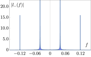
Fig. 20 shows the power spectrum for a representative $\mathbb{Z}_{2}$-symmetric limit cycle at $\delta=0.44$ and $W=0.056$ in the rotating frame. This frequency comb has peaks at $\pm f_{0},\pm 3f_{0},\pm 5f_{0},\cdots$, where $f_{0}\approx 0.040$ is the fundamental frequency. To estimate the value of $f_{0}$ in SI units, recall that in our units $N\Gamma_{c}=1$. In a typical experiment there are about $N=10^{6}$ atoms inside the optical cavity. Representative values of the Rabi frequency $\Omega$ and the cavity decay rate $\kappa$ are $\Omega=$37 Hz and $\kappa=9.4\times 10^{5}$ Hz according to Ref. Holland_One_Ensemble_Theory_1, . Using these numbers, we calculate,

$$\mbox{$N\Gamma_{c}=1.4$ kHz},\quad\mbox{$f_{0}=0.040N\Gamma_{c}=56$ Hz,}$$ (98)

which is indeed 4 orders of magnitude smaller than $f_{\mathrm{mc}}$.

We numerically verify that $\mathbb{Z}_{2}$-symmetric limit cycles have the following time translation property:

$$s_{x,y}\left(t\pm\frac{T}{2}\right)=-s_{x,y}(t),\quad s_{z}\left(t\pm\frac{T}{2}\right)=s_{z}(t).$$ (99)

This property explains why the power spectrum consists only of odd harmonics. We prove this by Fourier transforming the two sides of the equation $l_{-}(t)=l_{-}(t+T/2)$. Eq. (99) also holds for the analytical solutions in Eqs. (69) and (74). Since the $\mathbb{Z}_{2}$ symmetric limit cycle elsewhere is topologically connected to the one near the $W=1$ line, it also retains the above property. However, note that Eq. (99) is different from a related property (90) of limit cycles without $\mathbb{Z}_{2}$ symmetry. Eq. (99) is valid for any choice of $x$ and $y$-axes. On the other hand, Eq. (90) implies that $s_{y}(t)$ changes sign when shifted by half a period, while $s_{x}(t)$ does not, in a special coordinate frame rotated by $\phi_{0}$ around the $z$-axis.

Moreover, because of the $\mathbb{Z}_{2}$ symmetry $l_{y}(t)=0$ and $l_{x}(t)=2s_{x}(t)$ in a suitable coordinate system [see the text above Eq. (16)], i.e., $l_{-}(t)$ is a real function. As a result the power spectrum has a reflection symmetry about $f=0$,

$$|l_{-}(f)|^{2}=|l_{-}(-f)|^{2}.$$ (100)

One can infer more about the power spectra where analytical solutions exist. The harmonic solution from Sect. IV.1.1 entails prominent peaks at $\pm f_{0}$, where $f_{0}$ in various limits is,

$$W \rightarrow 1:\quad f_{0}=\frac{\sqrt{\delta^{2}-1}}{4\pi},$$ (101a)

$$W \rightarrow 0:\quad f_{0}=\frac{\delta}{4\pi},$$ (101b)

$$\delta \gg 1:\quad f_{0}=\frac{\sqrt{\delta^{2}-W^{2}}}{4\pi}.$$ (101c)

Near $\delta=W=1$ the solution is in terms of the Jacobi elliptic function cn. According to Eqs. (74) and (70), $l_{x}(t)=2s_{x}(t)=\frac{2aW}{\delta}\mathrm{cn}(bt,k)$. The function cn has the following series expansion Abramowitz_Stegun ; Gradshteyn_Ryzhik :

$$\textrm{cn}u=\frac{2\pi}{kK(k)}\sum_{n=1}^{\infty}\frac{q^{n-\frac{1}{2}}}{1-q^{2n-1}}\cos{\bigg{[}(2n-1)\frac{\pi u}{2K(k)}\bigg{]}}.$$ (102)

where $q=e^{-\frac{\pi K(k^{\prime})}{K(k)}}$ and $k^{\prime}=\sqrt{1-k^{2}}$. In our case,

$$u\equiv bt=\frac{\sqrt{|r|}t}{\sqrt{2|1-2k^{2}|}},$$ (103)

where $r=\delta-1$ and we used Eq. (75). This again corroborates the appearance of only odd harmonics in the power spectrum at $\pm f_{0},\pm 3f_{0},\pm 5f_{0},\cdots$, where $f_{0}$ is

$$f_{0}=\frac{\sqrt{|r|}}{4K(k)\sqrt{2\left|1-2k^{2}\right|}}.$$ (104)

Expressions (101) and (104) demonstrate that the frequency $f_{0}$ and, therefore, the spacing between peaks in the power spectrum, can take any value from 0 to $\infty$ depending on $\delta$ and $W$. In particular, for $\delta$ and $W$ of order 1, $f_{0}\sim 0.1N\Gamma_{c}$ close to the value in Eq. (98).

V.2.2 $\mathbb{Z}_{2}$-Symmetry-Broken Limit Cycle

Figure 21: Power spectrum for a $\mathbb{Z}_{2}$-symmetry-broken limit cycle at $(\delta,W)=(0.42,0.056)$. Unlike in the $\mathbb{Z}_{2}$-symmetric spectrum, both even and odd peaks are present. The fundamental frequency is $f_{0}\approx 0.038$. The most pronounced peak is at $f=0$.

Figure 22: Power spectrum for a $\mathbb{Z}_{2}$-symmetry-broken limit cycle at $(\delta,W)=(0.23,0.056)$. In contrast to Fig. 21, the reflection symmetry of the power spectrum is completely lost and the carrier frequency is shifted to a negative value from $f=0$.

In Fig. 21, we show the power spectrum of a $\mathbb{Z}_{2}$-symmetry-broken limit cycle at $\delta=0.42$ and $W=0.056$ in the rotating frame. Unlike for the $\mathbb{Z}_{2}$-symmetric limit cycle, both odd and even harmonics are present, i.e., peaks are at $0,\pm f_{0},\pm 2f_{0},\cdots$ The most pronounced peak is at zero. This is because of the loss of the time translation property (99).

Moreover, here $l_{y}(t)\neq 0$ and as a result $l_{-}(t)$ is complex. Thus, $l_{-}(f)$ does not obey Eq. (100) and the spectra no longer have reflection symmetry about the $f=0$ axis. However, notice that the spectrum in Fig. 21 still seems to have retained this symmetry. We explain this based on our numerical observation that for these values of $\delta$ and $W,$ in a suitably rotated frame,

$$l_{y}(t)=l_{y0}+\textrm{small oscillations},$$ (105)

where $l_{y0}$ is a constant complex number. In the Fourier transform of $l_{-}(t)=l_{x}(t)+\imath l_{y}(t)$, $l_{x}(t)$ produces a symmetric spectrum, $l_{y0}$ contributes only to the peak at $f=0$, and the small oscillations lead to a small asymmetry. As a result, although a careful analysis of the peak heights shows that the reflection symmetry of the power spectrum is in fact broken, this is hard to discern from Fig. 21.

In contrast, the $\mathbb{Z}_{2}$-symmetry-broken limit cycle in Fig. 22 is visibly asymmetric with respect to the $f=0$ axis. Furthermore, it features an offset of all frequencies originating from the $\omega_{q}t$ term (overall precession) in the net phase $\Phi(t)$ discussed in detail in Sect. IV.3. Specifically, Eq. (95) implies that the power spectrum of such limit cycles is $f_{q}+pf_{0},$ where $p$ is an arbitrary integer, $f_{q}=\omega_{q}/2\pi$, and $f_{0}$ is the frequency of the limit cycle.

VI Discussion

In this paper, we studied the long time dynamics of two atomic ensembles (clocks) in an optical cavity and constructed the nonequilibrium phase diagram for this system shown in Fig. 1. In the extreme bad cavity regime, we adiabatically eliminated the cavity degrees of freedom to obtain an effective master equation in terms of the atomic operators only. Further, we performed a consistent system size expansion for the master equation to derive the mean-field equations of motion and the Fokker-Planck equation governing quantum fluctuations. Mean-field time evolution is in terms of two collective classical spins representing individual ensembles. Each nonequilibrium phase in Fig. 1 corresponds to a distinct attractor (asymptotic solution) of the mean-field dynamics.

Mean-field equations of motion for two ensembles have two symmetries: an axial symmetry about the $z$-axis and a $\mathbb{Z}_{2}$ symmetry with respect to an interchange of the two ensembles. The phase diagram features spontaneous breaking of one or both of these symmetries.

There are two types of fixed points – the trivial steady state or TSS (normal nonradiative phase), and the nontrivial steady state or NTSS (monochromatic superradiance). Using linear stability analysis, we obtained their basins of attraction as Phases I and II in Fig. 1. Both of them lose stability via Hopf bifurcations. Going beyond the linear stability analysis, by deriving the Poincaré-Birkhoff normal form, we proved that the TSS goes through a supercritical Hopf bifurcation on the boundary of Phases I and III, whereas the NTSS undergoes a subcritical Hopf bifurcation on the II-III boundary. Thus, II to III and I to III transitions are analogous to the first and second order phase transitions, respectively. This analysis also explains the coexistence region near the boundary of Phases II and III.

After bifurcation, the TSS gives rise to a $\mathbb{Z}_{2}$-symmetric limit cycle (periodically modulated superradiance). We were able to derive analytical solutions for this limit cycle in terms of harmonic or Jacobi elliptic functions in several parts of Phase III. Moreover, we have shown with Floquet analysis that the $\mathbb{Z}_{2}$-symmetric limit cycle becomes unstable on the symmetry breaking line (the dashed line in Fig. 1) to bring about two distinct $\mathbb{Z}_{2}$-symmetry-broken limit cycles.

Experimentally, one distinguishes between different dynamical phases of the two ensembles by measuring the power spectrum of the light radiated by the cavity. In particular, the NTSS emits monochromatic light at a certain frequency $f_{\mathrm{mc}}$. Limit cycles emit frequency combs – series of equidistant peaks at $f_{\mathrm{mc}}+pf_{0}$, where $p$ is an integer and $f_{0}$ is the limit cycle frequency. For a $\mathbb{Z}_{2}$-symmetric limit cycle, $p$ is always odd, while for $\mathbb{Z}_{2}$-symmetry-broken limit cycles it takes arbitrary integer values. Certain symmetry-broken limit cycles also renormalize the value of $f_{\mathrm{mc}}$ relative to the NTSS and produce power spectra that are asymmetric about the $f=0$ axis. We estimated typical values of $f_{0}$ from available experimental data and found that it is several orders of magnitude smaller than $f_{\mathrm{mc}}$. Therefore, an interesting feature of limit cycles from the point of view of applications to ultrastable lasers is that they provide access to a range of frequencies drastically different from the atomic transition (lasing) frequency.

Here we have not analyzed more complicated time-dependent solutions to the left of the dashed line in Fig. 1 marking the spontaneous breaking of the $\mathbb{Z}_{2}$ symmetry. After the loss of the symmetry between the two ensembles, one needs to consider all six mean-field equations of motion (three for each classical spin) together. According to the Poincaré-Benedixson theorem, a system of three or more coupled first-order ordinary differential equations admits chaos. Indeed, we show in Refs. Patra_2, ; Patra_3, that chaos emerges by way of quasiperiodicity in our system. Moreover, eventually the chaotic time dependence of one of the clocks synchronizes with that of the other via on-off intermittency. The transition from chaos to chaotic synchronization is an example of spontaneous restoration of the $\mathbb{Z}_{2}$ symmetry.

Making system parameters, such as pump rates and numbers of atoms, unequal for the two ensembles naturally destroys the $\mathbb{Z}_{2}$ symmetry of the mean-field equations of motion with respect to the interchange of the ensembles. Nevertheless, we verified numerically that for a weak asymmetry in system parameters the long time dynamics of the two ensembles remain close to that in our nonequilibrium phase diagram in Fig. 1 and exhibit the same main phases. For example, a nearly $\mathbb{Z}_{2}$-symmetric limit cycle replaces the $\mathbb{Z}_{2}$-symmetric limit cycle in Phase III etc.

Let us also briefly discuss how the mean-field dynamics changes when the cavity decay rate $\kappa$ is not extremely large. Note that although one cannot adiabatically eliminate the photon degrees of freedom in this case, the fixed points are identical to the ones obtained in the bad cavity limit. The dynamics, however, lead to higher dimensional phase diagrams. For example, in the single ensemble setup, the semiclassical equations for fixed $N$ (number of atoms in the ensemble) have two dimensionless parameters and can be mapped to the Lorenz equation Carmichael_1 . Thus, even the single ensemble equations lead to periodic and chaotic asymptotic solutions. For two ensembles, we do not anticipate any new kinds of asymptotic solutions other than fixed points, limit cycles, quasiperiodicity, and chaos. However, the mechanisms that give rise to different phases (especially chaos and chaotic synchronization) and the corresponding stability analyses are expected to be more complicated.

It would be interesting to explore the many-body version of our system with $n\gg 1$ atomic ensembles identically coupled to a heavily damped cavity mode. It is simple to check that the TSS and NTSS survive in the many-body case. At zero pumping, the evolution equations (4) for $n$ ensembles resemble mean-field equations of motion for the $s$-wave Bardeen-Cooper-Schrieffer (BCS) superconductor in terms of classical Anderson pseudospins. Here too individual spins couple through the $x$ and $y$ components of the total spin. The main difference is that BCS dynamics are Hamiltonian and integrable yuzbashyan2005 . Nevertheless, there are many similarities between the nonequilibrium phase diagram in Fig. 1 and many-body quantum quench phase diagrams of BCS superconductors ydgf . In particular, the latter contain three phases closely analogous to Phases I-III in Fig. 1. Here the amplitude of the superconducting order parameter, which is the analog of $|l_{-}(t)|$, either asymptotes to zero (Phase I) or to a finite constant (Phase II) or oscillates periodically (Phase III), see Ref. jasen, for more on this similarity between the phase diagrams.

Another interesting problem, especially in the many-body context, is to analyze the dynamics beyond mean-field and determine if the full master equation supports truly quantum attractors inaccessible to the semiclassical dynamics Vakulchyk . Recent work has also pointed out an interpretation of limit cycles in atom-cavity systems as boundary time crystals saro . Alternatively, one can consider the same two atomic ensembles, but place them inside a multimode cavity to see if new types of correlated behaviors emerge in this setup Multimode .

Appendix A Nonequilibrium Phase Diagram for a Single Atomic Clock

Here we show that the nonequilibrium phase diagram for a single atomic clock maps to the $\delta=0$ axis of the two-clock diagram in Fig. 1. Therefore, there are only two phases in this case – the normal phase with no radiation (TSS), and monochromatic superradiance (NTSS), see also Refs. Holland_One_Ensemble_Theory_1, ; Holland_One_Ensemble_Theory_2, ; Holland_One_Ensemble_Expt_1, . We will also show that the mean-field evolution equations in this case reduce to damped Toda oscillator.

For one ensemble, the evolution equations (4) read,

$$\dot{s}_{-} = \biggl{(}-\imath\omega_{1}-\frac{W}{2}\biggr{)}s_{-}+\frac{1}{2}s_{z}s_{-},$$ (106a)

$$\dot{s}_{z} = W\big{(}1-s_{z}\big{)}-\frac{1}{2}s_{+}s_{-}.$$ (106b)

Going to a uniformly rotating frame, $s_{-}\to s_{-}e^{-\imath\omega_{1}t}$ and $s_{z}\to s_{z}$, we eliminate $\omega_{1}$ from Eq. (106a), i.e.,

$$\dot{s}_{-} = -\frac{W}{2}s_{-}+\frac{1}{2}s_{z}s_{-},$$ (107a)

$$\dot{s}_{z} = W\big{(}1-s_{z}\big{)}-\frac{1}{2}s_{+}s_{-}.$$ (107b)

Now consider Eq. (4) for two ensembles with $\omega_{A}=-\omega_{B}=\delta/2$ at detuning $\delta=0$. Summing these equations over $\tau$, we obtain

$$\dot{l}_{-} = -\frac{W}{2}l_{-}+\frac{1}{2}l_{z}l_{-},$$ (108a)

$$\dot{l}_{z} = W\big{(}2-l_{z}\big{)}-\frac{1}{2}l_{+}l_{-}.$$ (108b)

After rescaling $\bm{l}\to 2\bm{s},W\to 2W$ and $2t\to t$, these equations coincide with Eq. (107). The scaling factor of 2 arises because Eq. (108) describes a single ensemble with $2N$ atoms, while Eq. (107) is for $N$ atoms.

On the other hand, Eq. (108) corresponds to two ensembles at $\delta=0$. Thus, the phases are those on the vertical $\delta=0$ axis in Fig. 1, i.e., $l_{-}=2s_{-}$ asymptotes to its value in the TSS or NTSS for $\delta=0$. Therefore, the nonequilibrium phase diagram for a single atomic clock is 1D with the following two phases:

$$\begin{array}[]{llll}\mbox{TSS:}&s_{-}=0,&\quad s_{z}=1&\mbox{for $W>1;$}\\ \mbox{NTSS:}&s_{-}=e^{-\imath\Phi}\sqrt{2W(1-W)},&\quad s_{z}=W,&\mbox{for $W<1,$ }\\ \end{array}$$ (109)

where $\Phi$ is arbitrary. We derive these expressions directly from Eqs. (17) and (18) by replacing $l_{\perp}\to 2s_{\perp}$, $W\to 2W$, and setting $\delta=0$.

Let us also analyze the transient mean-field dynamics of a single atomic clock. Using $s_{-}=s_{\perp}e^{-\imath\Phi}$ in Eq. (107a) and separating it into real and imaginary parts, we find that $\dot{\Phi}=0$. Eq. (107) becomes,

$$s_{z}=\frac{2\dot{s}_{\perp}}{s_{\perp}}+W,\quad\dot{s}_{z}=W\big{(}1-s_{z}\big{)}-\frac{s_{\perp}^{2}}{2}.$$ (110)

Making the substitution $s_{\perp}=e^{X/2}$, we obtain $s_{z}=\dot{X}+W$ and the second order differential equation for $X$,

$$\ddot{X}+W\dot{X}+\frac{e^{X}}{2}+W(W-1)=0.$$ (111)

This equation describes the damped Toda oscillator Toda . It has been studied with Painlevé analysis and argued to be nonintegrable unless the last term in Eq. (111) is twice the square of the damping coefficient toda1 . In our case, this condition of integrability reads $W(W-1)=2W^{2},$ i.e., $W=0$ or $W=-1$. The case $W=0$ is straightforward to solve. It corresponds to the origin, $\delta=W=0$, of the two clock phase diagram and we solve it in Appendix C.1. The case $W=-1$ is unphysical in our context. Thus, dynamics in the presence of pumping are nonintegrable already for one bad cavity ensemble.

Appendix B Derivation of the Poincaré-Birkhoff Normal Form

We established in Sect. III.1.4 that the reduced equations of motion (16) determine the stability of the TSS and NTSS. In this appendix we derive the corresponding Poincaré-Birkhoff normal forms, i.e., the right hand side of Eq. (62), starting from Eq. (16). We closely follow the steps in Ref. Intro_bifurc, , but fix a number of mistakes along the way and in the final answer.

A key ingredient in this construction is the center manifold. Recall that in a Hopf bifurcation two complex conjugate characteristic values cross the imaginary line and acquire positive real parts. In this case, it is sufficient to study the dynamics projected onto a 2D center manifold. Imagine all the limit cycles as they continuously change their shape and size upon changing a parameter, such as $\delta$ or $W$. Heuristically, the center manifold is the 2D sheet (this can be sufficiently warped away from the bifurcation) made by putting these limit cycles one after the other. This manifold is tangent to the plane defined by the two unstable characteristic directions at the bifurcation. For a pitchfork bifurcation, where a real characteristic value becomes positive and there is a single unstable characteristic direction, the center manifold is 1D.

B.1 Hopf Bifurcation of the TSS and NTSS

The main steps of the derivation of the Poincaré-Birkhoff normal form for a Hopf bifurcation are as follows:

1. Shift the origin of the coordinate system to the fixed point.

2. Perform a linear transform $\bm{s}\to{\bm{s}}^{\prime}$ such that Eq. (16) takes the form

   $$\frac{d{\bm{s}}^{\prime}}{dt}=\big{[}\underbrace{\textrm{Block diagonal linear part}}_{(2\times 2)\bigoplus(1\times 1)}\big{]}\cdot{\bm{s}}^{\prime}+\textrm{ Second or higher order terms},$$ (112)

   where the $2\times 2$ part corresponds to the dynamics in the center manifold ($s_{x}^{\prime},s_{y}^{\prime}$).

3. Since the center manifold is 2D, parameterize $s_{z}^{\prime}$ in terms of the other two spin components near criticality,

   $$s_{z}^{\prime}=h(s_{x}^{\prime},s_{y}^{\prime}).$$ (113)

   Using this, produce the effective part of the dynamics projected onto the center manifold. This is still not the Poincaré-Birkhoff normal form. It contains all (including the non-essential) nonlinear terms.

4. Write the equations in terms of $s^{\prime}_{\pm}=s^{\prime}_{x}\pm\imath s^{\prime}_{y}$.

5. Perform the “near identity transformation”. This is a smooth change of variables $s^{\prime}_{\pm}\to s^{\prime\prime}_{\pm}$ that simplifies the $k$th and higher order terms in projected dynamical equations. For Hopf bifurcations, it is possible to eliminate even order nonlinear terms in this way (nonessential terms for this bifurcations). Carrying out this transformation up to the second order, we obtain the coefficient $a_{1}$ in front of $s^{3}$ in the Poincaré-Birkhoff normal form as written in Eq. (62).

B.1.1 Center Manifold Reduction

We start by shifting the origin of the coordinate system to the fixed point $\bm{s}_{0}$ in Eq. (16),

$$\dot{s}_{x} = \bigg{(}s_{z0}-\frac{W}{2}\bigg{)}s_{x}-\frac{\delta}{2}s_{y}+s_{x0}s_{z}+s_{z}s_{x},$$ (114a)

$$\dot{s}_{y} = \frac{\delta}{2}s_{x}-\frac{W}{2}s_{y},$$ (114b)

$$\dot{s}_{z} = -2s_{x0}s_{x}-Ws_{z}-s^{2}_{x}.$$ (114c)

Although the fixed point is now at $(0,0,0)$, the Jacobian matrix (60) remains the same. Let $\lambda_{r}$ ($v_{1}$) and $\gamma\pm\imath\omega$ ($v_{r}\pm\imath v_{i}$) be the real and complex characteristic values (vectors) at a Hopf bifurcation. Explicitly, for the bifurcation of the TSS on the $W=1,\delta\geq 1$ half-line, we read off $\lambda_{r}$, $\gamma$, and $\omega$ from Eq. (49) and the characteristic vectors are,

$$v_{1}=\begin{pmatrix}[1.5]0\\ 0\\ 1\end{pmatrix},\qquad v_{r}=\begin{pmatrix}[1.5]1\\ \delta\\ 0\end{pmatrix},\qquad v_{i}=\begin{pmatrix}[1.5]\sqrt{\delta^{2}-1}\\ 0\\ 0\end{pmatrix}.$$ (115)

Similarly, for the bifurcation of the NTSS on the II-III boundary $\lambda_{r}$ and $\gamma\pm\imath\omega$ are the roots of the polynomial $P_{3}(\lambda)$ in Eq. (52b), while the characteristic vectors read,

$$v_{1}=\begin{pmatrix}[1.5]\lambda_{r}+W\\ \delta\bigg{(}\frac{\lambda_{r}+W}{2\lambda_{r}+W}\bigg{)}\ \\ -2s_{x0}\end{pmatrix},\qquad v_{r}=\begin{pmatrix}[1.5]\gamma+W\\ \frac{\delta\big{[}(2\gamma+W)(\gamma+W)+2\omega^{2}\big{]}}{\big{[}(2\gamma+W)^{2}+4\omega^{2}\big{]}}\\ -2s_{x0}\end{pmatrix},\qquad v_{i}=\begin{pmatrix}[1.5]\omega\\ \frac{-W\omega\delta}{\big{[}(2\gamma+W)^{2}+4\omega^{2}\big{]}}\\ 0\end{pmatrix},$$ (116)

Next, we perform a linear transformation that block-diagonalizes the Jacobian into $2\times 2$ and $1\times 1$ blocks,

$$\begin{pmatrix}s_{x}\\ s_{y}\\ s_{z}\end{pmatrix}=\mathbb{Q}_{H}\cdot\begin{pmatrix}s^{\prime}_{x}\\ s^{\prime}_{y}\\ s^{\prime}_{z}\end{pmatrix},$$ (117)

where $\mathbb{Q}_{H}=(v_{r}\;v_{i}\;v_{1})$. Using the above relation in Eq. (114), we obtain,

$$\begin{pmatrix}[1.5]\dot{s}^{\prime}_{x}\\ \dot{s}^{\prime}_{y}\end{pmatrix} = \begin{pmatrix}[1.5]\gamma&\omega\\ -\omega&\gamma\end{pmatrix}\begin{pmatrix}[1.5]s^{\prime}_{x}\\ s^{\prime}_{y}\end{pmatrix}+\begin{pmatrix}[1.5]R_{1}\big{(}s^{\prime}_{x},s^{\prime}_{y},s^{\prime}_{z}\big{)}\\ R_{2}\big{(}s^{\prime}_{x},s^{\prime}_{y},s^{\prime}_{z}\big{)}\end{pmatrix},$$ (118a)

$$\dot{s}^{\prime}_{z} = \lambda_{r}s^{\prime}_{z}+R_{3}\big{(}s^{\prime}_{x},s^{\prime}_{y},s^{\prime}_{z}\big{)},$$ (118b)

where,

$$R_{i}\big{(}s^{\prime}_{x},s^{\prime}_{y},s^{\prime}_{z}\big{)}=R_{i1}\big{(}s^{\prime}_{x}\big{)}^{2}+R_{i2}\big{(}s^{\prime}_{y}\big{)}^{2}+R_{i3}s^{\prime}_{x}s^{\prime}_{y}+R_{i4}s^{\prime}_{x}s^{\prime}_{z}+R_{i5}s^{\prime}_{y}s^{\prime}_{z}+R_{i6}\big{(}s^{\prime}_{z}\big{)}^{2}.$$ (119)

Note, $R_{ij}$ for all $i$ and $j$ are known functions of $\delta$ and $W$.

Near the fixed point $(0,0,0)$ we parameterize the center manifold through $s^{\prime}_{z}\equiv h\big{(}s^{\prime}_{x},s^{\prime}_{y}\big{)}$. Since the fixed point belongs to the manifold and the $s^{\prime}_{x}\!\!-\!\!s^{\prime}_{y}$ plane is tangential to it at $(0,0,0)$, we have,

$$h(0,0)=0,\qquad\frac{\partial h}{\partial s^{\prime}_{x}}\bigg{|}_{(0,0)}=0,\qquad\frac{\partial h}{\partial s^{\prime}_{y}}\bigg{|}_{(0,0)}=0.$$ (120)

This implies,

$$h\big{(}s^{\prime}_{x},s^{\prime}_{y}\big{)}=h_{1}\big{(}s^{\prime}_{x}\big{)}^{2}+h_{2}\big{(}s^{\prime}_{y}\big{)}^{2}+h_{3}s^{\prime}_{x}s^{\prime}_{y}+\mathcal{O}\left(|\bm{s}^{\prime}_{\perp}|^{3}\right).$$ (121)

Substituting $s^{\prime}_{z}=h(s^{\prime}_{x},s^{\prime}_{y})$ into Eq. (118), we derive,

$$\begin{pmatrix}[1.5]\frac{\partial h}{\partial s^{\prime}_{x}}&\frac{\partial h}{\partial s^{\prime}_{y}}\end{pmatrix}\begin{bmatrix}[1.5]\begin{pmatrix}[1.5]\gamma&\omega\\ -\omega&\gamma\end{pmatrix}\begin{pmatrix}[1.5]s^{\prime}_{x}\\ s^{\prime}_{y}\end{pmatrix}+\begin{pmatrix}[1.5]R_{1}\\ R_{2}\end{pmatrix}\end{bmatrix}=\lambda_{r}h\big{(}s^{\prime}_{x},s^{\prime}_{y}\big{)}+R_{3}.$$ (122)

Now using the form of $h\big{(}s^{\prime}_{x},s^{\prime}_{y}\big{)}$ in Eq. (121) and equating the coefficients of $\big{(}s^{\prime}_{x}\big{)}^{2},\big{(}s^{\prime}_{y}\big{)}^{2}$ and $s^{\prime}_{x}s^{\prime}_{y}$ on both sides, we solve for $h_{1},h_{2}$ and $h_{3}$ as follows:

$$h_{1}=\frac{h_{3}\omega+R_{31}}{2\gamma-\lambda_{r}},\qquad h_{2}=\frac{-h_{3}\omega+R_{32}}{2\gamma-\lambda_{r}},\qquad h_{3}=\frac{2\omega(R_{32}-R_{31})+(2\gamma-\lambda_{r})R_{33}}{(2\gamma-\lambda_{r})^{2}+4\omega^{2}}.$$ (123)

Finally, the effective equation projected on the center manifold is,

$$\begin{pmatrix}[1.5]\dot{s}^{\prime}_{x}\\ \dot{s}^{\prime}_{y}\end{pmatrix}=\begin{pmatrix}[1.5]\gamma&\omega\\ -\omega&\gamma\end{pmatrix}\begin{pmatrix}[1.5]s^{\prime}_{x}\\ s^{\prime}_{y}\end{pmatrix}+\begin{pmatrix}[1.5]R_{11}\big{(}s^{\prime}_{x}\big{)}^{2}+R_{12}\big{(}s^{\prime}_{y}\big{)}^{2}+R_{13}s^{\prime}_{x}s^{\prime}_{y}\\ R_{21}\big{(}s^{\prime}_{x}\big{)}^{2}+R_{22}\big{(}s^{\prime}_{y}\big{)}^{2}+R_{23}s^{\prime}_{x}s^{\prime}_{y}\end{pmatrix}+\\ +\bigg{(}h_{1}\big{(}s^{\prime}_{x}\big{)}^{2}+h_{2}\big{(}s^{\prime}_{y}\big{)}^{2}+h_{3}s^{\prime}_{x}s^{\prime}_{y}\bigg{)}\begin{pmatrix}[1.5]R_{14}s^{\prime}_{x}+R_{15}s^{\prime}_{y}\\ R_{24}s^{\prime}_{x}+R_{25}s^{\prime}_{y}\end{pmatrix}+\mathcal{O}\left(|s^{\prime}_{-}|^{4}\right).$$ (124)

B.1.2 The Normal Form

The next step is to rewrite Eq. (124) in terms of $s^{\prime}_{\pm}=s^{\prime}_{x}\pm\imath s^{\prime}_{y}$,

$$\begin{pmatrix}[1.5]\dot{s}^{\prime}_{+}\\ \dot{s}^{\prime}_{-}\end{pmatrix}=\underbrace{\begin{pmatrix}[1.5](\gamma-\imath\omega)s^{\prime}_{+}\\ (\gamma+\imath\omega)s^{\prime}_{-}\end{pmatrix}}_{V^{(1)}\big{(}s^{\prime}_{+},s^{\prime}_{-}\big{)}}+\underbrace{\begin{pmatrix}[1.5]R^{(2,0)}_{+}\big{(}s^{\prime}_{-}\big{)}^{2}+R^{(2,1)}_{+}s^{\prime}_{-}s^{\prime}_{+}+R^{(2,2)}_{+}\big{(}s^{\prime}_{-}\big{)}^{2}\\ R^{(2,0)}_{-}\big{(}s^{\prime}_{-}\big{)}^{2}+R^{(2,1)}_{-}s^{\prime}_{+}s^{\prime}_{-}+R^{(2,2)}_{-}\big{(}s^{\prime}_{+}\big{)}^{2}\end{pmatrix}}_{V^{(2)}\big{(}s^{\prime}_{+},s^{\prime}_{-}\big{)}}+\\ +\underbrace{\begin{pmatrix}[1.5]R^{(3,0)}_{+}\big{(}s^{\prime}_{-}\big{)}^{3}+R^{(3,1)}_{+}s^{\prime}_{+}\big{(}s^{\prime}_{-}\big{)}^{2}+R^{(3,2)}_{+}\big{(}s^{\prime}_{+}\big{)}^{2}s^{\prime}_{-}+R^{(3,3)}_{+}\big{(}s^{\prime}_{+}\big{)}^{3}\\ R^{(3,0)}_{-}\big{(}s^{\prime}_{-}\big{)}^{3}+R^{(3,1)}_{-}s^{\prime}_{+}\big{(}s^{\prime}_{-}\big{)}^{2}+R^{(3,2)}_{-}\big{(}s^{\prime}_{+}\big{)}^{2}s^{\prime}_{-}+R^{(3,3)}_{-}\big{(}s^{\prime}_{+}\big{)}^{3}\end{pmatrix}}_{V^{(3)}\big{(}s^{\prime}_{+},s^{\prime}_{-}\big{)}}+\mathcal{O}\left(|s^{\prime}_{-}|^{4}\right),$$ (125)

where $V^{(k)}:\mathbb{R}^{2}\longrightarrow\mathbb{R}^{2}$ are homogeneous polynomial maps of degree $k=1,2,3,\ldots$. Hence, for $a\in\mathbb{R}$ one has $V^{(k)}\big{(}as^{\prime}_{+},as^{\prime}_{-}\big{)}=a^{k}V^{(k)}\big{(}s^{\prime}_{+},s^{\prime}_{-}\big{)}$. At this point it is helpful to introduce the following basis functions for $V^{(k)}$:

$$\left.\begin{array}[]{l}\xi^{{(k,l)}}_{+}=\begin{pmatrix}[1.5]s_{+}^{l}s_{-}^{k-l}\\ 0\end{pmatrix},\\[25.0pt] \xi^{{(k,l)}}_{-}=\begin{pmatrix}[1.5]0\\ s_{+}^{l}s_{-}^{k-l}\end{pmatrix},\end{array}\right\}\qquad\text{$l$ = 0, 1, \ldots, $k$.}$$ (126)

From the definitions of $R_{\pm}^{(k,l)}$ in Eq. (125), it is clear that they are nothing but the coefficients of different $\xi^{{(k,l)}}_{\pm}$, i.e.,

$$V^{(k)}=\sum_{l=0}^{k}R_{+}^{(k,l)}\xi^{(k,l)}_{+}+\sum_{l=0}^{k}R_{-}^{(k,l)}\xi^{(k,l)}_{-}.$$ (127)

We read off these coefficients $R_{\pm}^{(k,l)}$ from Eqs. (125) and (124) as,

$$R_{+}^{(3,0)}=\left[R_{-}^{(3,3)}\right]^{*} =\frac{1}{8}\big{[}h_{1}\big{(}R_{14}-R_{25}\big{)}+h_{2}\big{(}R_{25}-R_{14}\big{)}-h_{3}\big{(}R_{15}+R_{24}\big{)}\big{]}+$$

$$\qquad\qquad\qquad\qquad\qquad+\frac{\imath}{8}\big{[}\big{(}h_{1}-h_{2}\big{)}\big{(}R_{15}+R_{24}\big{)}+h_{3}\big{(}R_{14}+R_{25}\big{)}\big{]},$$ (128a)

$$R_{+}^{(3,1)}=\left[R_{-}^{(3,2)}\right]^{*} =\frac{1}{8}\big{[}3\big{(}h_{1}R_{14}-h_{2}R_{25}\big{)}+h_{2}R_{14}+h_{3}R_{15}-h_{3}R_{24}-h_{1}R_{25}\big{]}+$$

$$\qquad\qquad\qquad\quad+\frac{\imath}{8}\big{[}3\big{(}h_{2}R_{15}+h_{1}R_{24}\big{)}+h_{3}R_{14}+h_{1}R_{15}+h_{2}R_{24}+h_{3}R_{25}\big{]},$$ (128b)

$$R_{+}^{(3,2)}=\left[R_{-}^{(3,1)}\right]^{*} =\frac{1}{8}\big{[}3\big{(}h_{1}R_{14}+h_{2}R_{25}\big{)}+h_{2}R_{14}+h_{3}R_{15}+h_{3}R_{24}+h_{1}R_{25}\big{]}+$$

$$\qquad\qquad\qquad\quad+\frac{\imath}{8}\big{[}3\big{(}h_{1}R_{24}-h_{2}R_{15}\big{)}+h_{2}R_{24}+h_{3}R_{25}-h_{3}R_{14}+h_{1}R_{15}\big{]},$$ (128c)

$$R_{+}^{(3,3)}=\left[R_{-}^{(3,0)}\right]^{*} =\frac{1}{8}\big{[}h_{3}\big{(}-R_{15}+R_{24}\big{)}+h_{1}\big{(}R_{14}+R_{25}\big{)}-h_{2}\big{(}R_{14}+R_{25}\big{)}\big{]}+$$

$$\qquad\qquad\qquad\qquad\qquad+\frac{\imath}{8}\big{[}-\big{(}h_{1}-h_{2}\big{)}\big{(}R_{15}-R_{24}\big{)}-h_{3}\big{(}R_{14}+R_{25}\big{)}\big{]},$$ (128d)

$$R_{+}^{(2,0)}=\left[R_{-}^{(2,2)}\right]^{*} =\frac{1}{4}\big{(}R_{11}-R_{12}-R_{23}\big{)}+\frac{\imath}{4}\big{(}R_{13}+R_{21}-R_{22}\big{)},$$ (128e)

$$R_{+}^{(2,1)}=\left[R_{-}^{(2,1)}\right]^{*} =\frac{1}{2}\big{(}R_{11}+R_{12}\big{)}+\frac{\imath}{2}\big{(}R_{21}+R_{22}\big{)},$$ (128f)

$$R_{+}^{(2,2)}=\left[R_{-}^{(2,0)}\right]^{*} =\frac{1}{4}\big{(}R_{11}-R_{12}+R_{23}\big{)}+\frac{\imath}{4}\big{(}R_{21}-R_{13}-R_{22}\big{)}.$$ (128g)

Next, we eliminate as many nonlinear terms as possible from Eq. (125). To achieve this, we introduce the following transformation:

$$\begin{pmatrix}[1.5]s^{\prime}_{+}\\ s^{\prime}_{-}\end{pmatrix}=\begin{pmatrix}[1.5]s^{\prime\prime}_{+}\\ s^{\prime\prime}_{-}\end{pmatrix}-\begin{pmatrix}[1.5]\phi^{(k)}_{s^{\prime\prime}_{+}}\big{(}s^{\prime\prime}_{+},s^{\prime\prime}_{-}\big{)}\\ \phi^{(k)}_{s^{\prime\prime}_{-}}\big{(}s^{\prime\prime}_{+},s^{\prime\prime}_{-}\big{)}\end{pmatrix},\qquad\phi^{(k)}\big{(}s^{\prime\prime}_{+},s^{\prime\prime}_{-}\big{)}\equiv\begin{pmatrix}[1.5]\phi^{(k)}_{s^{\prime\prime}_{+}}\big{(}s^{\prime\prime}_{+},s^{\prime\prime}_{-}\big{)}\\ \phi^{(k)}_{s^{\prime\prime}_{-}}\big{(}s^{\prime\prime}_{+},s^{\prime\prime}_{-}\big{)}\end{pmatrix},$$ (129)

where $\phi^{(k)}_{s^{\prime\prime}_{\pm}}\big{(}s^{\prime\prime}_{+},s^{\prime\prime}_{-}\big{)}$ are small homogeneous polynomials of order $k$. One needs to perform such near identity transformations iteratively. In particular, substituting Eq. (129) into Eq. (125) and using Taylor expansions for $V^{(2)}$ and $(\mathbb{1}-\mathbb{O})^{-1}=\mathbb{1}+\mathbb{O}+\mathbb{O}^{2}+\ldots$, we derive

$$\begin{pmatrix}[1.5]\dot{s}^{\prime\prime}_{+}\\ \dot{s}^{\prime\prime}_{+}\end{pmatrix}=V^{(1)}+\bigg{[}V^{(2)}-DV^{(1)}\cdot\phi^{(2)}+D\phi^{(2)}\cdot V^{(1)}\bigg{]}+\\ +\bigg{[}V^{(3)}-DV^{(2)}\cdot\phi^{(2)}+D\phi^{(2)}\cdot V^{(2)}-D\phi^{(2)}\cdot DV^{(1)}\cdot\phi^{(2)}+\left(D\phi^{(2)}\right)^{2}\cdot V^{(1)}\bigg{]}+\mathcal{O}\left(|s^{\prime\prime}_{-}|^{4}\right),$$ (130)

where

$$DV^{k}\equiv\begin{pmatrix}[2]\frac{\partial V^{k}_{+}}{\partial s^{\prime\prime}_{+}}&\frac{\partial V^{k}_{+}}{\partial s^{\prime\prime}_{-}}\\ \frac{\partial V^{k}_{-}}{\partial s^{\prime\prime}_{+}}&\frac{\partial V^{k}_{-}}{\partial s^{\prime\prime}_{-}}\end{pmatrix},\qquad\qquad D\phi^{k}\equiv\begin{pmatrix}[2]\frac{\partial\phi^{k}_{s^{\prime\prime}_{+}}}{\partial s^{\prime\prime}_{+}}&\frac{\partial\phi^{k}_{s^{\prime\prime}_{+}}}{\partial s^{\prime\prime}_{-}}\\ \frac{\partial\phi^{k}_{s^{\prime\prime}_{-}}}{\partial s^{\prime\prime}_{+}}&\frac{\partial\phi^{k}_{s^{\prime\prime}_{-}}}{\partial s^{\prime\prime}_{-}}\end{pmatrix}.$$ (131)

The modified nonlinear terms are

$$\widetilde{V}^{(2)} \equiv \bigg{[}V^{(2)}-DV^{(1)}\cdot\phi^{(2)}+D\phi^{(2)}\cdot V^{(1)}\bigg{]},$$ (132a)

$$\widetilde{V}^{(3)} \equiv \bigg{[}V^{(3)}-DV^{(2)}\cdot\phi^{(2)}+D\phi^{(2)}\cdot V^{(2)}-D\phi^{(2)}\cdot DV^{(1)}\cdot\phi^{(2)}+\left(D\phi^{(2)}\right)^{2}\cdot V^{(1)}\bigg{]}.$$ (132b)

Note, a near identity transformation at the $k$th order, alters terms of the $k$th and higher orders. In particular, the $k$th order term becomes

$$\widetilde{V}^{(k)}=V^{(k)}-DV^{(1)}\cdot\phi^{(k)}+D\phi^{(k)}\cdot V^{(1)}\equiv V^{(k)}-L\left(\phi^{(k)}\right),$$ (133)

where we have introduced a linear operator. A function $\phi^{(k)}$ satisfying

$$V^{(k)}=L\left(\phi^{(k)}\right),$$ (134)

eliminates the $k$th order nonlinear term. We verify that the eigenfunctions of $L$ are the column vectors $\xi^{{(k,l)}}_{\pm}$ defined in Eq. (126). The corresponding eigenvalues are

$$\lambda^{(k,l)}_{\pm}\equiv\gamma(1-k)-\imath\omega(k-2l\pm 1),\quad L\left(\xi^{{(k,l)}}_{\pm}\right)=\lambda^{(k,l)}_{\pm}\xi^{{(k,l)}}_{\pm}.$$ (135)

At criticality $(\gamma=0,\omega>0)$ one ends up with $\lambda^{(k,l)}_{\pm}=0$, if and only if $k=2l\mp 1$, i.e., when $k$ is odd. Moreover, $\lambda^{(k,l)}_{\pm}=0$ guarantees that one is unable to invert Eq. (134) to obtain $\phi^{(k)}$. Therefore, Eq. (134) does not have a solution if $k$ is odd and $V^{(k)}$ contains terms proportional to either $\xi^{{(k,\frac{k+1}{2})}}_{+}$ or $\xi^{{(k,\frac{k-1}{2})}}_{-}$, i.e., when $R_{\pm}^{(k,\frac{k\pm 1}{2})}\neq 0$ in Eq. (127). Such nonlinearities that cannot be eliminated with a near identity transformation are known as essential nonlinearities. We see that any $k$th order polynomial map is of the form $V^{(k)}=V^{(k)}_{r}+V^{(k)}_{c}$, where $V^{(k)}_{r}$ and $V^{(k)}_{c}$ are the removable (inessential) and essential nonlinearities.

Eq. (135) implies that to eliminate $V^{(2)}$ by the second order near identity transformation, we need

$$\phi^{(2)}=\sum_{l=0}^{2}\bigg{[}\frac{R_{+}^{(2,l)}}{\lambda_{+}^{2,l}}\xi_{+}^{(2,l)}+\frac{R_{-}^{(2,l)}}{\lambda_{-}^{2,l}}\xi_{-}^{(2,l)}\bigg{]}.$$ (136)

This introduces extra terms at the third and higher order. Similarly, the third order near identity transformation, such that $L\big{(}\phi^{(3)}\big{)}=\widetilde{V}^{(3)}_{r}$, eliminates the nonessential parts of $\widetilde{V}^{(3)}$ defined in Eq. (132). This transformation does not affect $\widetilde{V}^{(3)}_{c}=\alpha_{1}\xi^{{(3,2)}}_{+}+\alpha^{*}_{1}\xi^{{(3,1)}}_{-}$. Thus,

$$\alpha_{1}=R_{+}^{(3,2)}+R_{+}^{(2,1)}\left(\phi_{+}^{(2,2)}-\phi_{-}^{(2,1)}\right)+\phi_{+}^{(2,1)}\left(R_{-}^{(2,1)}-R_{+}^{(2,2)}\right)+2\left(R_{-}^{(2,2)}\phi_{+}^{(2,0)}-R_{+}^{(2,0)}\phi_{-}^{(2,2)}\right)+\gamma\left[2\phi_{-}^{(2,2)}\phi_{+}^{(2,0)}\right.+\\ +\left.\phi_{+}^{(2,1)}\left(\phi_{-}^{(2,1)}+3\phi_{+}^{(2,2)}\right)\right]+\imath\omega\left[\phi_{+}^{(2,1)}\left(\phi_{+}^{(2,2)}-\phi_{-}^{(2,1)}\right)-6\phi_{-}^{(2,2)}\phi_{+}^{(2,0)}\right],$$ (137)

where

$$\phi_{\pm}^{(2,l)}\equiv\frac{R_{\pm}^{(2,l)}}{\lambda_{\pm}^{(2,l)}}.$$ (138)

Substituting $s^{\prime\prime}_{\pm}=se^{\pm\imath\theta}$ into the resulting equations of motion, we obtain

$$\dot{s} = \gamma s+\mathrm{Re}(\alpha_{1})s^{3}+\mathcal{O}\big{(}s^{5}\big{)},$$ (139a)

$$\dot{\theta} = \omega-\mathrm{Im}(\alpha_{1})s^{2}+\mathcal{O}\big{(}s^{4}\big{)}.$$ (139b)

This is Eq. (62) with $a_{1}=\mathrm{Re}(\alpha_{1})$.

B.2 Pitchfork Bifurcation of the TSS

As we discussed at the end of Sect. III.1.4, the TSS loses stability via a pitchfork bifurcation in the reduced equations of motion (16) on the upper quarter-arc forming the boundary between phases I and II. In this case, the center manifold is 1D. We diagonalize the linear part of Eq. (114) with the following linear transformation:

$$\begin{pmatrix}s_{x}\\ s_{y}\\ s_{z}\end{pmatrix}=\mathbb{Q}_{P}\cdot\begin{pmatrix}s^{\prime}_{x}\\ s^{\prime}_{y}\\ s^{\prime}_{z}\end{pmatrix},$$ (140)

where $\mathbb{Q}_{P}=(v_{x^{\prime}}\;v_{y^{\prime}}\;v_{z^{\prime}})$, and $v_{x^{\prime}},v_{y^{\prime}}$ and $v_{z^{\prime}}$ are the eigenvectors of the Jacobian (60), where now $s_{x0}=0$ and $s_{z0}=1$. We wrote down the corresponding eigenvalues in Eq. (49), which we now rename as $\lambda_{x^{\prime}}\equiv\lambda_{3,4}$, $\lambda_{y^{\prime}}\equiv\lambda_{5,6}$, and $\lambda_{z^{\prime}}\equiv\lambda_{1,2}$. Explicitly, the eigensystem of the Jacobian matrix at the TSS reads,

$$\lambda_{x^{\prime}}= \frac{1}{2}\big{(}1-W+\sqrt{1-\delta^{2}}\big{)},\qquad \lambda_{y^{\prime}} =\frac{1}{2}\big{(}1-W-\sqrt{1-\delta^{2}}\big{)},\qquad \lambda_{z^{\prime}} =-W,$$ (141)

$$v_{x^{\prime}}= \begin{pmatrix}[1.5]\frac{1}{\delta}\big{(}1+\sqrt{1-\delta^{2}}\big{)}\\ 1\\ 0\end{pmatrix},\qquad v_{y^{\prime}} =\begin{pmatrix}[1.5]\frac{1}{\delta}\big{(}1-\sqrt{1-\delta^{2}}\big{)}\\ 1\\ 0\end{pmatrix},\qquad v_{z^{\prime}} =\begin{pmatrix}[1.5]0\\ 0\\ 1\end{pmatrix}.$$

Inside Phase II, $\lambda_{x^{\prime}}$ becomes positive. After the linear transformation (140), Eq. (114) becomes

$$\dot{s}^{\prime}_{x} = \lambda_{x^{\prime}}s^{\prime}_{x}+R_{1}\big{(}s^{\prime}_{x},s^{\prime}_{y},s^{\prime}_{z}\big{)},$$ (142a)

$$\dot{s}^{\prime}_{y} = \lambda_{y^{\prime}}s^{\prime}_{y}+R_{2}\big{(}s^{\prime}_{x},s^{\prime}_{y},s^{\prime}_{z}\big{)},$$ (142b)

$$\dot{s}^{\prime}_{z} = \lambda_{z^{\prime}}s^{\prime}_{z}+R_{3}\big{(}s^{\prime}_{x},s^{\prime}_{y},s^{\prime}_{z}\big{)}.$$ (142c)

Below we list the nonzero $R_{ij}$ using the same notation as in Eq. (119):

$$R_{14}=-R_{24}=\frac{1}{2}+\frac{1}{2\sqrt{1-\delta^{2}}},\quad R_{15}=-R_{25}=-\frac{1}{2}+\frac{1}{2\sqrt{1-\delta^{2}}},$$ (143)

$$R_{31}=-\frac{1}{\delta^{2}}\big{(}1+\sqrt{1-\delta^{2}}\big{)}^{2},\quad R_{32}=-\frac{1}{\delta^{2}}\big{(}1-\sqrt{1-\delta^{2}}\big{)}^{2},\quad R_{33}=-2.$$

Since the center manifold is 1D, we parametrize it as,

$$s^{\prime}_{y}=h_{1}(s^{\prime}_{x})^{2}+\cdots,\qquad s^{\prime}_{z}=g_{1}(s^{\prime}_{x})^{2}+\cdots.$$ (144)

This parameterization guarantees that the fixed point $s^{\prime}_{x}=s^{\prime}_{y}=s^{\prime}_{z}=0$ lies on the center manifold and the $s^{\prime}_{x}$-axis (the unstable characteristic direction) is tangential to it, cf. Eq. (120). Using Eq. (144) in Eqs. (142b) and (142c) and equating the coefficients of $s^{\prime}_{x}$ and $(s^{\prime}_{x})^{2}$ on both sides, we find

$$h_{1}=0,\quad g_{1}=\frac{R_{31}}{2\lambda_{x^{\prime}}-\lambda_{z^{\prime}}}=-\frac{1}{\delta^{2}}\big{(}1+\sqrt{1-\delta^{2}}\big{)}.$$ (145)

Finally, substituting the resulting $s^{\prime}_{y}$ and $s^{\prime}_{z}$ into Eq. (142a), we derive the normal form for this bifurcation as

$$\dot{s}^{\prime}_{x}=\lambda_{x^{\prime}}s^{\prime}_{x}+R_{14}g_{1}(s^{\prime}_{x})^{3}+\mathcal{O}\big{(}s^{4}\big{)}.$$ (146)

The coefficient of $(s^{\prime}_{x})^{3}$ is $-\frac{\big{(}1+\sqrt{1-\delta^{2}}\big{)}^{2}}{2\delta^{2}\sqrt{1-\delta^{2}}}<0$ proving that the TSS goes through a supercritical pitchfork bifurcation at the boundary between Phases I and II.

Appendix C Dynamics of Two Atomic Ensembles in a Bad Cavity in the Absence of Pumping

In this Appendix, we analyze the dynamics of our system without pumping, i.e., on the $W=0$ line of the nonequilibrium phase diagram in Fig. 1. Only attractors on this line are non-radiative fixed points. In fact, there is a family of such fixed points for each value of the detuning $\delta$, only one of which is continuously connected to the limit cycle living in the green region of Fig. 1 at $W\neq 0$. We will also see that in the absence of pumping, mean-field equations of motion (4) for an arbitrary number $n$ of ensembles are a set of generalized Landau-Lifshitz-Gilbert equations that conserve the lengths of the spins. Separately, we will study the dynamics for $\delta=W=0$, which reduces to the $W=0$ case of the one ensemble dynamics we considered in Appendix A.

At $W=0$ it is useful to rewrite the mean-field evolution equations (4) [or equivalently Eq. (31)] in a vector form as

$$\frac{d\bm{s}^{\tau}}{dt}=\omega_{\tau}\hat{z}\times\bm{s}^{\tau}+\frac{1}{2}\big{(}\hat{z}\times\bm{l}\big{)}\times\bm{s}^{\tau},\quad\bm{l}=\sum_{\tau}\bm{s}^{\tau}.$$ (147)

This is the Landau-Lifshitz-Gilbert equation LL ; gilbert for the total spin $\bm{l}$ when all $\omega_{\tau}$ are the same. Otherwise, it is an inhomogeneous variant of the latter. The Landau-Lifshitz-Gilbert damping term in Eq. (147) pushes the spins towards the $z$-axis whenever $\bm{l}\neq 0$. Eq. (147) conserves the magnitudes of classical spins $\bm{s}^{\tau}$ since

$$\bm{s}^{\tau}\cdot\frac{d\bm{s}^{\tau}}{dt}=0.$$ (148)

First, consider the case $\delta\neq 0$. We observe numerically that for a generic initial condition $\big{(}s^{A}_{x0},s^{A}_{y0},s^{A}_{z0},s^{B}_{x0},s^{B}_{y0},s^{B}_{z0}\big{)}$, the asymptotic solution for two atomic ensembles is $\big{(}0,0,-|\bm{s}^{A}_{0}|,0,0,-|\bm{s}^{B}_{0}|\big{)}$. By analyzing the eigenvalues of the Jacobian (46), we also establish that this fixed point is stable, while any other choice of signs of the $z$-components results in an unstable fixed point. Therefore, there is a family of stable fixed points labeled by $|\bm{s}^{A}_{0}|$ and $|\bm{s}^{B}_{0}|$ for each $\delta$ on the $W=0$ axis of the phase diagram, which are not $\mathbb{Z}_{2}$-symmetric and different from the TSS. According to Eq. (68), the $\mathbb{Z}_{2}$-symmetric limit cycle in $W\to 0$ limit turns into a fixed point $\bm{s}^{A}=\bm{s}^{B}=0$, which is only one member of the above family of fixed points.

C.1 The Origin of the Phase Diagram

Here we exactly solve the case $W=\delta=0$. In this case, the total spin satisfies Eq. (108) with $W=0$, which is the same as Eq. (107) at $W=0$. Therefore, it is legitimate to simply replace $\bm{s}$ with $\bm{l}$ and set $W=0$ in Eq. (110), i.e.,

$$l_{z}l_{\perp}=2\dot{l}_{\perp},\quad\dot{l}_{z}=-\frac{l_{\perp}^{2}}{2}.$$ (149)

Let $l_{\perp}=e^{X/2}$ to obtain the Toda oscillator equation,

$$\ddot{X}+\frac{e^{X}}{2}=0.$$ (150)

As discussed below Eq. (111), this equation is integrable. Its general solution is

$$l_{\perp}^{2}=\frac{2C^{2}_{1}}{1+\cosh{\big{[}C_{1}t+C_{2}\big{]}}},$$ (151)

where $C_{1}$ and $C_{2}$ are arbitrary constants. Eqs. (151) and (149) show that $l_{\perp}\to 0$ and $l_{z}\to\mathrm{const}$ as $t\to+\infty$.

Then, Eq. (31), where now $W=0$ and $\omega_{A}=-\omega_{B}=\delta/2=0$, implies that the time derivatives $\dot{s}^{\tau}_{x},\dot{s}^{\tau}_{y}$ and $\dot{s}^{\tau}_{z}$ vanish since $l_{\perp}\to 0$ at large times. Thus, the asymptotic solution for an arbitrary initial condition $\big{(}s^{A}_{x0},s^{A}_{y0},s^{A}_{z0},s^{B}_{x0},s^{B}_{y0},s^{B}_{z0}\big{)}$ is

$$s^{A}_{x}(\infty) =-s^{B}_{x}(\infty)=s_{x\infty},$$ (152a)

$$s^{A}_{y}(\infty) =-s^{B}_{y}(\infty)=s_{y\infty},$$ (152b)

$$s^{\tau}_{z}(\infty) =\pm\sqrt{|\bm{s}^{\tau}_{0}|^{2}-s_{x\infty}^{2}-s_{y\infty}^{2}},\quad\tau=A,B.$$ (152c)

In the last equation we took into account that the spin length is conserved in the absence of pumping. The choice of signs in Eq. (152c) depends on the initial condition, but should be such that $l_{z}\leq 0$. Indeed, a linear stability analysis with the Jacobian (46) reveals that fixed points (152) are unstable when $l_{z}>0$ and stable when $l_{z}<0$. These fixed points are distinct from the TSS and generally do not retain the $\mathbb{Z}_{2}$ symmetry.

One describes the resultant dynamics as follows. Start with two arbitrary pointing spin vectors. Since $\delta=0$, $\omega_{\tau}=0$ in Eq. (147) and the spins do not precess. Due to the Landau-Lifshitz-Gilbert damping, both spins are pushed towards the $z$-axis. Eventually, they align in such a way that $l_{x}=l_{y}=0$ and $l_{z}\leq 0$. At that point all the time derivatives vanish and the spins get stuck.

Appendix D Power Spectrum of Radiated Electric Field

In this appendix, we show that the emission spectrum of atomic ensembles coupled through a heavily damped cavity mode is proportional to $|l_{-}(f)|^{2}$, where $l_{-}(f)$ is defined in Eq. (23). Our derivation combines the approaches of Refs. Carmichael_1, ; Carmichael_3, . For simplicity, we examine a ring cavity at $z=0$ coupled to a 1D reservoir of length $\mathsf{L}$, which is a collection of standing waves with nodes at $\pm\mathsf{L}/2$. The Hamiltonian is,

$$\hat{H}=\hat{H}_{S}+\hat{H}_{R}+\hat{H}_{SR},$$ (153)

where,

$$\hat{H}_{S}=\omega_{0}\hat{a}^{\dagger}\hat{a},\quad\hat{H}_{R}=\sum_{j}\omega_{j}\hat{r}_{j}^{\dagger}\hat{r}_{j},\quad\hat{H}_{SR}=\sum_{j}\big{(}\kappa_{j}^{*}\hat{a}\hat{r}_{j}^{\dagger}+\kappa_{j}\hat{a}^{\dagger}\hat{r}_{j}\big{)},$$ (154)

and $\hat{a}(\hat{a}^{\dagger})$ and $\hat{r}_{j}(\hat{r}_{j}^{\dagger})$ are the annihilation (creation) operators for the cavity and the reservoir modes, respectively. The periodic boundary condition allows us to replace the sum over $\omega_{j}$ with an integration over $\omega$ with the density of states $g(\omega)=\mathsf{L}/2\pi c$, where $c$ is the speed of light. Assuming the reservoir is in the state of thermal equilibrium at temperature $T_{0}$ and adopting the Born-Markov approximation, we obtain the following master equation:

$$\dot{\rho}=-\imath\omega_{0}\big{[}\hat{a}^{\dagger}\hat{a},\rho\big{]}+\underbrace{\kappa(1+\bar{n})\mathcal{L}[\hat{a}]\rho}_{\textrm{Emission}}+\underbrace{\kappa\bar{n}\mathcal{L}[\hat{a}^{\dagger}]\rho}_{\textrm{Absorption}},$$ (155)

where $\bar{n}\equiv\frac{\exp{(-\omega_{0}/k_{B}T_{0})}}{1-\exp{(-\omega_{0}/k_{B}T_{0})}}$, $\kappa\equiv 2\pi g(\omega_{0})|\kappa(\omega_{0})|^{2}=\Xi c/2\mathsf{L}$ and $\Xi<1$ is the transmission coefficient of the mirror separating the cavity from its surrounding. At temperatures close to 0 K, we neglect all terms proportional to $\bar{n}$ in Eq. (155). As a result, we are left only with the spontaneous emission of the cavity mode as shown in Eq. (1). We also neglect the Lamb shift.

The measurable output electric field in terms of the reservoir operators reads,

$$\hat{\textbf{E}}(z,t)=\hat{\textbf{E}}^{(+)}(z,t)+\hat{\textbf{E}}^{(-)}(z,t),$$ (156)

where,

$$\hat{\textbf{E}}^{(+)}(z,t)\equiv\imath\hat{e}_{0}\sum_{k}\sqrt{\frac{\omega_{k}}{2\varepsilon_{0}\mathsf{A}\mathsf{L}}}\hat{r}_{k}(t)e^{\imath\omega_{k}z/c+\zeta(z)},\quad\hat{\textbf{E}}^{(-)}(z,t)\equiv\hat{\textbf{E}}^{(+)}(z,t)^{\dagger}.$$ (157)

The phase shift $\zeta(z)$ due to the mirror separating the cavity from the reservoir is $\zeta(z)=\zeta_{R}$ for $z>0$ and zero otherwise. The unit vector $\hat{e}_{0}$ is perpendicular to the $z$-axis and $A$ is the cross-sectional area of the cavity mode.

To relate the evolution of the reservoir modes $\hat{r}_{k}(t)$ to that of the cavity mode $\hat{a}(t)$, consider the equation of motion for $\hat{r}_{k}(t)$,

$$\dot{\hat{r}}_{k}(t)=-\imath\omega_{k}\hat{r}_{k}(t)-\imath\kappa_{k}^{*}\hat{a}(t).$$ (158)

The solution of the above equation is

$$\hat{r}_{k}(t)=\hat{r}_{k}(0)e^{-\imath\omega_{k}t}-\imath\kappa_{k}^{*}\int_{0}^{t}dt^{\prime}\hat{a}(t)e^{\imath\omega_{k}(t^{\prime}-t)}.$$ (159)

Eq. (157) becomes

$$\hat{\textbf{E}}^{(+)}(z,t)=\hat{\textbf{E}}^{(+)}_{f}(z,t)+\hat{\textbf{E}}^{(+)}_{s}(z,t).$$ (160)

Here $\hat{\textbf{E}}^{(+)}_{f}(z,t)$ is the freely evolving part of the electric field involving only $\hat{r}_{k}$ and $\hat{\textbf{E}}^{(+)}_{s}(z,t)$ originating from the second term on the right hand side of Eq. (159) describes the effect of the cavity. We are interested in the autocorrelation function,

$$\mathrm{Auto}(\tau)=\int_{-\infty}^{+\infty}dt\;\left\langle\hat{\textbf{E}}^{(-)}(z,t+z/c)\hat{\textbf{E}}^{(+)}(z,t+z/c+\tau)\right\rangle,$$ (161)

where the angular brackets denote taking a trace over the system and the reservoir degrees of freedom. At low temperatures the state of the reservoir is very close to the vacuum electromagnetic field, $\bar{n}(\omega_{j},T_{0})\approx 0$. Therefore, the contribution of the freely evolving part of the electric field is negligible, i.e.,

$$\left\langle\hat{\textbf{E}}^{(-)}(z,t+z/c)\hat{\textbf{E}}^{(+)}(z,t+z/c+\tau)\right\rangle\approx\left\langle\hat{\textbf{E}}^{(-)}_{s}(z,t+z/c)\hat{\textbf{E}}^{(+)}_{s}(z,t+z/c+\tau)\right\rangle.$$ (162)

Following the steps outlined in Sect. 1.4 of Ref. Carmichael_3, , we obtain,

$$\hat{\textbf{E}}^{(+)}_{s}(z,t)=\begin{cases}\hat{e}_{0}\sqrt{\frac{\omega_{0}}{2\varepsilon_{0}\mathsf{A}c}}\sqrt{2\kappa}e^{\imath\zeta_{R}}\hat{a}(t-z/c),&\text{if }ct>z>0\\ 0,&\text{if }z<0\end{cases}$$ (163)

According to Eq. (30) in the bad cavity limit,

$$\langle\hat{a}(t)\rangle\propto l_{-}(t).$$ (164)

Outside of the cavity, using Eqs. (163), (164) and the mean-field approximation in Eqs. (161) and (162), we derive,

$$\mathrm{Auto}(\tau)\propto\int_{-\infty}^{+\infty}dt\;l_{+}(t)l_{-}(t+\tau).$$ (165)

Finally, the Fourier transform of the autocorrelation function (the power spectrum) is,

$$\mathrm{Auto}(f)\propto|l_{-}(f)|^{2},$$ (166)

where we used the Wiener-Khintchine theorem.

References

- (1) R. H. Dicke, Coherence in Spontaneous Radiation Processes, Phys. Rev. 93, 99 (1954).
- (2) K. Hepp and E. Lieb, On the superradiant phase transition for molecules in a quantized radiation field: the Dicke maser model, Ann. Phys. 76, 360 (1973).
- (3) Y. K. Wang and F. T. Hioe, Phase Transition in the Dicke Model of Superradiance, Phys. Rev. A 7, 831 (1973).
- (4) H.J. Carmichael, C.W. Gardiner and D.F. Walls, Higher order corrections to the Dicke superradiant phase transition, Phys. Lett. A 46, 47 (1973).
- (5) P. Domokos and H. Ritsch, Collective Cooling and Self-Organization of Atoms in a Cavity, Phys. Rev. Lett. 89, 253003 (2002).
- (6) J. K. Asbóth, P. Domokos, H. Ritsch, and A. Vukics, Self-organization of atoms in a cavity field: Threshold, bistability, and scaling laws, Phys. Rev. A 72, 053417 (2005).
- (7) S. Gopalakrishnan, B. L. Lev and P. M. Goldbart, Atom-light crystallization of Bose-Einstein condensates in multimode cavities: Nonequilibrium classical and quantum phase transitions, emergent lattices, supersolidity, and frustration, Phys. Rev. A 82, 043612 (2010).
- (8) R. Bonifacio, L. De Salvo, L. M. Narducci, and E. J. D’Angelo, Exponential gain and self-bunching in a collective atomic recoil laser, Phys. Rev. A 50, 1716 (1994).
- (9) P. R. Berman, Comparison of recoil-induced resonances and the collective atomic recoil laser, Phys. Rev. A 59, 585 (1999).
- (10) D. Kruse, C. von Cube, C. Zimmermann, and Ph. W. Courteille, Observation of Lasing Mediated by Collective Atomic Recoil, Phys. Rev. Lett. 91, 183601 (2003).
- (11) K. Rzażewski, K. Wódkiewicz, and W. Żakowicz, Phase Transitions, Two-Level Atoms, and the Term, Phys. Rev. Lett. 35, 432 (1975).
- (12) F. Dimer, B. Estienne, A. S. Parkins, and H. J. Carmichael, Proposed realization of the Dicke-model quantum phase transition in an optical cavity QED system, Phys. Rev. A 75, 013804 (2007).
- (13) K. Baumann, C. Guerlin, F. Brennecke, and T. Esslinger, Dicke quantum phase transition with a superfluid gas in an optical cavity, Nature 464, 1301 (2010).
- (14) J. Keeling, M. J. Bhaseen, and B. D. Simons, Collective Dynamics of Bose-Einstein Condensates in Optical Cavities, Phys. Rev. Lett. 105, 043001 (2010).
- (15) K. Baumann, R. Mottl, F. Brennecke, and T. Esslinger, Exploring Symmetry Breaking at the Dicke Quantum Phase Transition, Phys. Rev. Lett. 107, 140402 (2011).
- (16) B. Öztop, M. Bordyuh, Ö. E. Müstecaplıoğlu and B. D. Simons, Collective Dynamics of Bose-Einstein Condensates in Optical Cavities, New J. Phys. 14, 085011 (2012).
- (17) M. J. Bhaseen, J. Mayoh, B. D. Simons, and J. Keeling, Dynamics of nonequilibrium Dicke models, Phys. Rev. A. 85, 013817 (2012).
- (18) E. G. Dalla Torre, S. Diehl, M. D. Lukin, S. Sachdev, and P. Strack, Keldysh approach for nonequilibrium phase transitions in quantum optics: Beyond the Dicke model in optical cavities, Phys. Rev. A 87, 023831 (2013).
- (19) F. Piazza, P. Strack, W. Zwerger, Bose-Einstein Condensation versus Dicke-Hepp-Lieb Transition in an Optical Cavity, Ann. Phys. 339, 135 (2013).
- (20) H. Ritsch, P. Domokos, F. Brennecke, and T. Esslinger, Cold atoms in cavity-generated dynamical optical potentials, Rev. Mod. Phys. 85, 553 (2013).
- (21) R. I. Moodie, K. E. Ballantine, J. Keeling, Generalized classes of continuous symmetries in two-mode Dicke models, Phys. Rev. A 97, 033802 (2018).
- (22) D. Nagy and P. Domokos, Nonequilibrium Quantum Criticality and Non-Markovian Environment: Critical Exponent of a Quantum Phase Transition, Phys. Rev. Lett. 115, 043601 (2015).
- (23) J. Klinder, H. Keßler, M. Reza Bakhtiari, M. Thorwart and A. Hemmerich, Observation of a superradiant Mott insulator in the Dicke-Hubbard model, Phys. Rev. Lett. 115, 230403 (2015).
- (24) E. G. Dalla Torre, Y. Shchadilova, E. Y. Wilner, M. D. Lukin, and E. Demler, Dicke phase transition without total spin conservation, Phys. Rev. A 94, 061802(R) (2016).
- (25) P. Kirton and J. Keeling, Suppressing and Restoring the Dicke Superradiance Transition by Dephasing and Decay, Phys. Rev. Lett. 118, 123602 (2017).
- (26) J. Gelhausen, M. Buchhold, and P. Strack, Many-body quantum optics with decaying atomic spin states: Dicke model, Phys. Rev. A 95, 063824 (2017).
- (27) P. Kirton and J. Keeling, Superradiant and Lasing States in Driven-Dissipative Dicke Models, New J. Phys. 20, 015009 (2018).
- (28) D. Meiser, Jun Ye, D. R. Carlson and M. J. Holland, Prospects for a Milihertz- Linewidth Laser, Phys. Rev. Lett. 102, 163601 (2009).
- (29) D. Meiser and M. J. Holland, Steady-state superradiance with alkaline-earth-metal atoms, Phys. Rev. A 81, 033847 (2010).
- (30) J. G. Bohnet, Z. Chen, J. M. Weiner, D. Meiser, M. J. Holland and J. K. Thompson, A steady-state superradiant laser with less than one intracavity photon, Nature 484, 78 (2012).
- (31) M. A. Norcia and J. K. Thompson, Cold-Strontium Laser in the Superradiant Crossover Regime, Phys. Rev. X 6, 011025 (2016).
- (32) Minghui Xu and M. J. Holland, Conditional Ramsey Spectroscopy with Synchronized Atoms, Phys. Rev. Lett. 114, 103601 (2015).
- (33) M. Wouters and I. Carusotto, Excitations in a Nonequilibrium Bose-Einstein Condensate of Exciton Polaritons, Phys. Rev. Lett. 99, 140402 (2007).
- (34) M. Wouters, I. Carusotto, and C. Ciuti, Spatial and spectral shape of inhomogeneous nonequilibrium exciton-polariton condensates, Phys. Rev. B 77, 115340 (2008).
- (35) J. Keeling and N. G. Berloff, Spontaneous Rotating Vortex Lattices in a Pumped Decaying Condensate, Phys. Rev. Lett. 100, 250401 (2008).
- (36) E. Wertz, L. Ferrier, D. D. Solnyshkov, P. Senellart, D. Bajoni, A. Miard, A. Lemaitre, G. Malpuech, and J. Bloch, Spontaneous formation of a polariton condensate in a planar GaAs microcavity, Appl. Phys. Lett. 95(5), 051108 (2009).
- (37) J. Kasprzak, M. Richard, S. Kundermann, A. Baas, P. Jeambrun, J. M. J. Keeling, F. M. Marchetti, M. H. Szymanska, R. André, J. L. Staehli, V. Savona, P. B. Littlewood, B. Deveaud, and L. S. Dang, Bose-Einstein condensation of exciton polaritons, Nature 443, 409 (2006).
- (38) R. Balili, V. Hartwell, D. Snoke, L. Pfeiffer, and K. West, Bose-Einstein Condensation of Microcavity Polaritons in a Trap, Science 316, 1007 (2007).
- (39) C. W. Lai, N. Y. Kim, S. Utsunomiya, G. Roumpos, H. Deng, M. D. Fraser, T. Byrnes, P. Recher, N. Kumada, T. Fujisawa and Y. Yamamoto, Coherent zero-state and -state in an exciton-polariton condensate array, Nature 450, 529 (2007).
- (40) I. L. Aleiner, B. L. Altshuler, and Y. G. Rubo, Radiative coupling and weak lasing of exciton-polariton condensates, Phys. Rev. B 85, 121301(R) (2012).
- (41) H. Ohadi, R. L. Gregory, T. Freegarde, Y. G. Rubo, A. V. Kavokin and P. G. Lagoudakis, Dissipative phase locking of exciton-polariton condensates, Phys. Rev. X 6, 031032 (2016).
- (42) K. Rayanov, B. L. Altshuler, Y. G. Rubo, and S. Flach, Frequency Combs with Weakly Lasing Exciton-Polariton Condensates, Phys. Rev. Lett. 114, 193901 (2015).
- (43) I.Y. Chestnov, S.S. Demirchyan, S.M. Arakelian, A.P. Alodjants, Y.G. Rubo and A.V. Kavokin, Permanent Rabi oscillations in coupled exciton-photon systems with PT symmetry, Scientific Reports 6, 19551 (2016).
- (44) Minghui Xu, D. A. Tieri, E. C. Fine, James K. Thompson and M. J. Holland, Synchronization of Two Ensembles of Atoms, Phys. Rev. Lett. 113, 154101 (2014).
- (45) A. Roth and K. Hammerer, Synchronization of active atomic clocks via quantum and classical channels, Phys. Rev. A 94, 043841 (2016).
- (46) J. M. Weiner, K. C. Cox, J. G. Bohnet, and J. K. Thompson, Phase synchronization inside a superradiant laser, Phys. Rev. A 95, 033808 (2017).
- (47) N. Shammah, S. Ahmed, N. Lambert, S. De Liberato, and F. Nori, Open quantum systems with local and collective incoherent processes: Efficient numerical simulation using permutational invariance, arXiv:1805.05129 (2018)
- (48) A. Pikovsky, M. Rosenblum and J. Kurths, Synchronization: A Universal Concept in Nonlinear Sciences, Cambridge Nonlinear Science Series, Vol. 12 (Cambridge University Press, Cambridge, UK, 2003).
- (49) A. Patra, B. L. Altshuler and E. A. Yuzbashyan, Driven-Dissipative Dynamics of Atomic Ensembles in a Resonant Cavity II: Quasiperiodic Route to Chaos and Chaotic Synchronization, arXiv:1909.01687.
- (50) A. Patra, B. L. Altshuler and E. A. Yuzbashyan, Chaotic Synchronization between Atomic Clocks, Phys. Rev. A 100, 023418 (2019).
- (51) J. D. Crawford, Introduction to bifurcation theory, Rev. Mod. Phys. 63, 991 (1991).
- (52) Y. A. Kuznetsov, Elements of Applied Bifurcation Theory, 2nd ed. (Springer-Verlag, New York, 1998).
- (53) R. C. Hilborn, Chaos and Nonlinear Dynamics, An Introduction for Scientists and Engineers, 2nd ed. (Oxford University Press, New York, 2001).
- (54) A. D. Ludlow, M. M. Boyd, T. Zelevinsky, S. M. Foreman, S. Blatt, M. Notcutt, T. Ido, and J. Ye, Systematic Study of the Clock Transition in an Optical Lattice, Phys. Rev. Lett. 96, 033003 (2006).
- (55) R. Bonifacio, P. Schwendimann, and Fritz Haake, Quantum Statistical Theory of Superradiance. I, Phys. Rev. A 4, 302 (1971).
- (56) H. J. Carmichael, Statistical Methods in Quantum Optics 1 - Master Equations and Fokker-Planck Equations (Springer-Verlag Berlin Heidelberg, 1999).
- (57) H. J. Carmichael, Statistical Methods in Quantum Optics 2 - Non-Classical Fields (Springer-Verlag, 2008).
- (58) H. J. Carmichael, An Open System Approach to Quantum Optics (Springer-Verlag, 1993).
- (59) R. J. Glauber, Coherent and Incoherent States of the Radiation Field, Phys. Rev. 131, 2766 (1963).
- (60) E. C. G. Sudarshan, Equivalence of Semiclassical and Quantum Mechanical Descriptions of Statistical Light Beams, Phys. Rev. Lett. 10, 277 (1963).
- (61) Since a pair of complex conjugate characteristic values acquire positive real parts, this is a double-Hopf bifurcation. When , all four of these characteristic values have same imaginary parts at criticality – making it a resonant Hopf bifurcation. This brings out the innate codimension 2 (in terms of and ) nature of the bifurcation.
- (62) I. S. Gradshteyn, and I. M. Ryzhik, Table of Integrals, Series, and Products, 7th English ed. (Academic Press, New York, 2007).
- (63) M. Abramowitz, and I Stegun, Handbook of Mathematical Functions with Formulas, Graphs, and Mathematical Tables, United States Department of Commerce, National Bureau of Standards (Dover Publications, New York, 1964).
- (64) Note that in Eq. (69) , whereas here we find . This is not a contradiction, because while solving for Eqs. (63) and (73) we have not fixed the origin of time. By suitably choosing the origin in one of the solutions, one can match the phases of the two functions exactly.
- (65) E. A. Yuzbashyan, B. L. Altshuler, V. B. Kuznetsov, and V. Z. Enolskii, Nonequilibrium Cooper pairing in the nonadiabatic regime, Phys. Rev. B 72, 220503(R) (2005).
- (66) E. A. Yuzbashyan, M. Dzero, V. Gurarie and M. S. Foster, Quantum quench phase diagrams of an -wave BCS-BEC condensate, Phys. Rev. A 91, 033628 (2015).
- (67) J. A. Scaramazza, P. Smacchia, E. A. Yuzbashyan, Consequences of integrability breaking in quench dynamics of pairing Hamiltonians, Phys. Rev. B 99, 054520 (2019).
- (68) I. Vakulchyk, I. Yusipov, M. Ivanchenko, S. Flach and S. Denisov, Signatures of many-body localization in steady states of open quantum systems, Phys. Rev. B 98, 020202(R) (2018).
- (69) F. Iemini, A. Russomanno, J. Keeling, M. Schirò, M. Dalmonte, and R. Fazio, Boundary Time Crystals, Phys. Rev. Lett. 121, 035301 (2018)
- (70) V. Vaidya, Y. Guo, R. Kroenze, K. Ballentine, A. Köllar, J. Keeling and B. Lev, Tunable-Range, Photon-Mediated Atomic Interactions in Multimode Cavity QED, Phys. Rev. X 8, 011002 (2018).
- (71) M. Toda, Theory of Nonlinear Lattices (Springer-Verlag, Berlin, Germany, 1988).
- (72) S. Parthasarathy and J. M. Dixon, Analytic structure and chaotic dynamics of the damped driven Toda oscillator, Phys. Rev. E 55, 3942 (1997).
- (73) L. D. Landau, E. M. Lifshitz, On the theory of the dispersion of magnetic permeability in ferromagnetic bodies, Phys. Z. Sowjet. 8, 153 (1935).
- (74) T. L. Gilbert, A phenomenological theory of damping in ferromagnetic materials, IEEE Trans. Mag. 40, 3443 (2004).