Theoretical and Experimental Analysis on the Generalizability of Distribution Regression Network

Abstract

There is emerging interest in performing regression between distributions. In contrast to prediction on single instances, these machine learning methods can be useful for population-based studies or on problems that are inherently statistical in nature. The recently proposed distribution regression network (DRN) (Kou et al., 2018) has shown superior performance for the distribution-to-distribution regression task compared to conventional neural networks. However, in Kou et al. (2018) and some other works on distribution regression, there is a lack of comprehensive comparative study on both theoretical basis and generalization abilities of the methods. We derive some mathematical properties of DRN and qualitatively compare it to conventional neural networks. We also perform comprehensive experiments to study the generalizability of distribution regression models, by studying their robustness to limited training data, data sampling noise and task difficulty. DRN consistently outperforms conventional neural networks, requiring fewer training data and maintaining robust performance with noise. Furthermore, the theoretical properties of DRN can be used to provide some explanation on the ability of DRN to achieve better generalization performance than conventional neural networks.

1 Introduction

There has been emerging interest in perform regression on complex inputs such as probability distributions. Performing prediction on distributions has many important applications. Many real-world systems are driven by stochastic processes. For instance, the Fokker-Planck equation (Risken, 1996) has been used to model a time-varying distribution, with applications such as astrophysics (Noble & Wheatland, 2011), biological physics (Guérin et al., 2011) and weather forecasting (Palmer, 2000). Extrapolating a time-varying distribution has also been used to train a classifier where the data distribution drifts over time (Lampert, 2015).

A recently proposed distribution regression model, distribution regression network (DRN) (Kou et al., 2018), outperforms conventional neural networks by proposing a novel representation of encoding an entire distribution in a single network node. On the datasets used by Kou et al. (2018), DRN achieves better accuracies with 500 times fewer parameters compared to the multilayer perceptron (MLP) and one-dimensional convolutional neural network (CNN). However, in Kou et al. (2018) and other distribution regression methods (Oliva et al., 2013, 2015), there is a lack of comprehensive comparative study on both theoretical basis and generalization abilities of the methods.

In this work, we derive some mathematical properties of DRN and qualitatively compare it to conventional neural networks. We also performed comprehensive experiments to study the generalizability of distribution regression models, by studying their robustness to limited training data, data sampling noise and task difficulty. DRN consistently outperforms conventional neural networks, requiring two to five times fewer training data to achieve similar generalization performance. With increasing data sampling noise, DRN’s performance remains robust whereas the neural network models saw more drastic decrease in test accuracy. Furthermore, the theoretical properties of DRN can be used to provide insights on the ability of DRN to achieve better generalization performance than conventional neural networks.

2 Related work

Various machine learning methods have been proposed for distribution data, ranging from distribution-to-real regression (Póczos et al., 2013; Oliva et al., 2014) to distribution-to-distribution regression (Oliva et al., 2015, 2013). The Triple-Basis Estimator (3BE) has been proposed for function-to-function regression. It uses basis representations of functions and learns a mapping from Random Kitchen Sink basis features (Oliva et al., 2015). 3BE shows improved accuracies for distribution regression compared to an instance-based learning method (Oliva et al., 2013). More recently, Kou et al. (2018) proposed the distribution regression network which extends the neural network representation such that an entire distribution is encoded in a single node. With this compact representation, DRN showed better accuracies while using much fewer parameters than conventional neural networks and 3BE (Oliva et al., 2015).

For predicting the future state of a time-varying distribution, Lampert (2015) proposed Extrapolating the Distribution Dynamics (EDD) which predicts the future state of a time-varying distribution given samples from previous time steps. EDD uses the reproducing kernel Hilbert space (RKHS) embedding of distributions and learns a linear mapping to model how the distribution evolves between adjacent time steps. EDD is shown to work for a few variants of synthetic data, but the performance deteriorates for tasks where the dynamics is non-linear.

3 Distribution Regression Network

For the distribution regression task, the dataset consists of $M$ data points $\mathcal{D}=\{(X_{1}^{1},\cdots,X_{1}^{K},Y_{1}),\cdots,(X_{M}^{1},\cdots,X_{M}^{K},Y_{M})\}$ where $X_{i}^{k}$ and $Y_{i}$ are univariate continuous distributions with compact support. The regression task is to learn the function $f$ which maps the input distributions to output distribution: $Y_{i}=f(X_{i}^{1},\cdots,X_{i}^{K})$ on unseen test data.

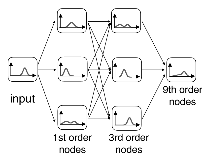
(a)

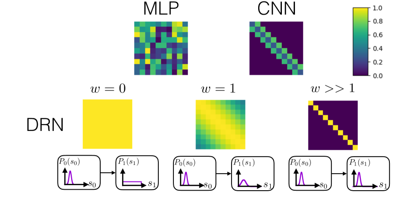
(b)

Figure 1: (a) DRN performs distribution regression by encoding each node with an entire distribution. Using multiple hidden layers, the DRN network shown has an output up with up to $9^{th}$ order transformation. (b) Visualization of the weight matrices for DRN, MLP and CNN where $q=10$. For DRN, we show different values of weight, along with the propagation behaviors.

Kou et al. (2018) proposed the distribution regression network (DRN) for the task of distribution-to-distribution regression. We give a brief description of DRN following the notations of Kou et al. (2018). Figure 1(a) shows that DRN consists of multiple fully-connected layers connecting the data input to the output in a feedforward manner, where each connection has a real-valued weight. The novelty of DRN is that each node in the network encodes a univariate probability distribution. The distribution at each node is computed using the distributions of the incoming nodes, the weights and the bias parameters. Let $P_{k}^{(l)}$ represent the probability density function (pdf) of the $k^{\text{th}}$ node in the $l^{\text{th}}$ layer where $P_{k}^{(l)}(s_{k}^{(l)})$ is the density of the distribution when the node variable is $s_{k}^{(l)}$. The unnormalized distribution $\tilde{P}_{k}^{(l)}$ is computed by marginalizing over the product of the unnormalized conditional probability and the incoming probabilities.

$$\tilde{P}_{k}^{(l)}\left(s_{k}^{(l)}\right)=\int_{\mathbf{s}^{(l-1)}}\tilde{Q}(s_{k}^{(l)}|\mathbf{s}^{(l-1)})P_{1}^{(l-1)}\left(s_{1}^{(l-1)}\right)\cdots P_{n}^{(l-1)}\left(s_{n}^{(l-1)}\right)\,d\mathbf{s}^{(l-1)},$$ (1)

where the shorthand $\mathbf{s}^{(l-1)}=s_{1}^{(l-1)}\cdots s_{n}^{(l-1)}$ is used for the incoming node variables and $\tilde{Q}(s_{k}^{(l)}|\mathbf{s}^{(l-1)})=\exp[-E(s_{k}^{(l)}|s_{1}^{(l-1)},\cdots,s_{n}^{(l-1)})]$. The unnormalized conditional probability has the form of the Boltzmann distribution, where $E$ is the energy for a given set of node variables,

$$E\left(s_{k}^{(l)}|\mathbf{s}^{(l-1)}\right)=\sum_{i}^{n}w_{ki}^{(l)}\left(\frac{s_{k}^{(l)}-s_{i}^{(l-1)}}{\Delta}\right)^{2}+b_{q,k}^{(l)}\left(\frac{s_{k}^{(l)}-\lambda_{q,k}^{(l)}}{\Delta}\right)^{2}+b_{a,k}^{(l)}\left|\frac{s_{k}^{(l)}-\lambda_{a,k}^{(l)}}{\Delta}\right|,$$ (2)

where $w_{ki}^{(l)}$ is the weight connecting the $i^{\text{th}}$ node in layer $l-1$ to the $k^{th}$ node in layer $l$. $b_{q,k}^{(l)}$ and $b_{a,k}^{(l)}$ are the quadratic and absolute bias terms acting on positions $\lambda_{q,k}^{(l)}$ and $\lambda_{a,k}^{(l)}$ respectively. $\Delta$ is the support length of the distribution. After obtaining the unnormalized probability, the distribution from Eq. (1) is normalized. Forward propagation is performed layer-wise to obtain the output prediction. The DRN propagation model, with the Boltzmann distribution, is motivated by work on spin models in statistical physics (Katsura, 1962; Lee et al., 2002). The distribution regression task is general and in this paper we extend it to the task of forward prediction on a time-varying distribution: Given a series of distributions with $T$ equally-spaced time steps, $X^{(1)},X^{(2)},\cdots,X^{(T)}$, we want to predict $X^{(T+k)}$, i.e. the distribution at $k$ time steps later. The input at each time step may consist of more than one distribution. To use DRN for the time series distribution regression, the input distributions for all time steps are concatenated at the input layer. The DRN framework is flexible and can be extended to architectures beyond feedforward networks. Since we are addressing the task of time series distribution regression, we also implemented a recurrent extension of DRN, which we call recurrent distribution regression network (RDRN). The extension is straightforward and we provide details of the architecture in the supplementary material.

Following Kou et al. (2018), the cost function for the prediction task is measured by the Jensen-Shannon divergence (Lin, 1991) between the label and predicted distributions. We adopt the same parameter initialization method as Kou et al. (2018), where the network weights and bias are randomly initialized following a uniform distribution and the bias positions are uniformly sampled from the support length of the data distribution. The integrals in Eq. (1) are performed numerically. Each continuous distribution density function is discretized into $q$ bins, resulting in a discrete probability mass function (i.e. a $q$-dimensional vector that sums to one).

4 Properties of DRN

DRN is able to perform transformations such as peak spreading and peak splitting, as discussed in detail in Kou et al. (2018). In this section, we provide further theoretical analysis on the functional form of DRN propagation which gives more insight to DRN’s generalization abilities. By expressing the integral in Eq. (1) with summation and the distribution at each node as a discretized $q$-length vector, we can express the output at a node in vector form, $\tilde{p}_{0}=B_{0}\circ(T_{w_{1}}\cdot p_{1})\circ(T_{w_{2}}\cdot p_{2})\circ\cdots\circ(T_{w_{n}}\cdot p_{n})=B_{0}\circ\breve{\prod}^{n}_{i=1}T_{w_{i}}\cdot p_{i},$ where $\breve{\prod}$ is a symbol for Hadamard products and upon normalization, $p_{0}=\tilde{p}_{0}/|\tilde{p}_{0}|$. $\circ$ is the element wise Hadamard product operator and $\cdot$ is the matrix multiplication operator. $B_{0}$ is a vector representing the bias term whose components are given by $(B_{0})_{i}=\exp\left(-b_{q}\left(\frac{s_{i}-\lambda_{q}}{\Delta}\right)^{2}-b_{a}\left|\frac{s_{i}-\lambda_{a}}{\Delta}\right|\right)$. $T_{w_{i}}$ is a symmetric $q$ by $q$ transformation matrix corresponding to the connections in DRN with elements $(T_{w_{i}})_{qr}=\exp\left(-w_{i}\left(\frac{s_{q}-s_{r}}{\Delta}\right)^{2}\right)$. With the Boltzmann distribution, under positive weight $w$, the matrix $T_{w_{i}}$ acts as a Gaussian filter on the input distribution, where $w$ controls the spread, as shown in Figure 1(b). In the following, we present some propositions concerning DRN, where their corresponding proofs are in the supplementary material.

Proposition 1.

A node connecting to a target node with zero weight $w=0$ has no effect on the activation of the target node.

Similar to conventional neural networks, this is a mechanism for which DRN can learn to ignore spurious nodes by setting their weights to zero or near zero.

Proposition 2.

For a node connecting to a target node with sufficiently large positive weight $w\to\infty$, the transformation matrix $T_{w}\to I$.

The consequence is that the identity mapping from one node to another can be realized.

Proposition 3.

Output of DRN is invariant to normalization of all hidden layers of DRN.

As an extension to Proposition 3, it can be shown that the output of DRN is invariant to scaling of the hidden layers. Therefore arbitrary scaling can be applied in the layers to control numerical stability. These normalization can be done dynamically during the computation. In this paper, we found that normalization of all layers is sufficient to provide the required numerical stability and precision for all our datasets.

Definition 1.

A node in DRN is said to be an order $n$ node when it is connected with non-zero weights from $n$ incoming nodes in the previous layer.

Lemma 1.

For an order $n$ node, components of $\tilde{p}_{0}$ (which we denote as $\tilde{p}_{0i}$), follow a power law of $n$th order cross terms of the components of connecting nodes.

$$\tilde{p}_{0i} = (B_{0})_{i}\sum_{j_{1}}\cdots\sum_{j_{n}}\underbrace{\left[(T_{w_{1}})_{i,j_{1}}\cdots(T_{w_{n}})_{i,j_{n}}\right]}_{\text{coefficients}}\underbrace{\left[(p_{1})_{j_{1}}\cdots(p_{n})_{j_{n}}\right]}_{\text{cross terms}}$$ (3)

Writing in short hand notation, $J^{(1)}=(j_{1},\cdots j_{n})$ where the superscript indicates $J$ is the indices over the first layer. Write $\sum_{j_{1}}\cdots\sum_{j_{n}}=\sum_{J^{(1)}}$ and consolidate the coefficients into a tensor, $c_{i,J^{(1)}}(w,B)=(B_{0})_{i}(T_{w_{1}})_{i,j_{1}}\cdots(T_{w_{n}})_{i,j_{n}}$, and the cross terms into a tensor, $P_{J^{(1)}}=(p_{1})_{j_{1}}\cdots(p_{n})_{j_{n}}$, where $w=(w_{1},\cdots w_{n})$. Eq. (3) can be written compactly as,

$$p_{0}=\sum_{J^{(1)}}c_{J^{(1)}}(w,B)P_{J^{(1)}}/\sum_{{\hat{J}}^{(1)}}z_{{\hat{J}}^{(1)}}(w,B)P_{{\hat{J}}^{(1)}}$$ (4)

where $p_{0}=(p_{01},p_{02},\cdots p_{0q})$, $c_{J^{(1)}}=(c_{1,J^{(1)}},\cdots c_{q,J^{(1)}})$, and $z_{{\hat{J}}^{(1)}}(w,B)=\sum_{i}c_{i,J^{(1)}}(w,B)$.

Using Proposition 3, we consider unnormalized hidden layers. The activations for the $\alpha^{th}$ node of the first hidden layer $h^{(1)}_{\alpha}$ and second hidden layer $h^{(2)}_{\alpha}$ are, $h^{(1)}_{\alpha}=\sum_{J^{(1)}_{\alpha}}c_{J^{(1)}_{\alpha}}P_{J^{(1)}_{\alpha}}$,

$h^{(2)}_{\alpha}=\sum_{J^{(2)}_{\alpha}}c_{J^{(2)}_{\alpha}}H_{J^{(2)}_{\alpha}}$ and $H_{J^{(2)}_{\beta}}=\prod_{\beta=1}^{n_{1}}\sum_{J^{(1)}_{\beta}}c_{j_{\beta},J^{(1)}_{\beta}}P_{J^{(1)}_{\beta}}$. Detailed derivations of the above equations are given in the supplementary material. Each of the $P_{J^{(1)}_{\beta}}$ consists of cross terms of the input distributions to order $n_{0}$ ($n_{0}$ is the number of input nodes). $H_{J^{(2)}_{\alpha}}$ is a product of $n_{1}$ terms of $P_{J^{(1)}_{\beta}}$’s, hence $H_{J^{(2)}_{\alpha}}$ will be cross terms of the input distributions to order $n_{1}\times n_{0}$. For a network of $L$ hidden layers with number of nodes, $n_{1},n_{2},\cdots n_{L}$, the output consist of multiplications of the components of input distributions to the power of $n_{0}\times n_{1}\cdots\times n_{L}$. In this way, DRN can fit high order functions exponentially quickly by adding hidden layers. For instance, the network in Figure 1(a) obtains a $9^{th}$ order transformation by using two hidden layers of only 3 nodes each.

Proposition 4.

For a node of order $n$, in the limit of small weights $|w_{\alpha}|\ll 1$ for $\alpha=1,\cdots n$, the output activions, ${p}_{0}$ can be approximated as a fraction of two linear combinations of the activations in the input nodes.

The consequence of proposition 4 is that by adjusting the weights and by expanding the matrix $T_{w_{\alpha}}$ to orders linear in $w_{\alpha}$, DRN can approximate the output distribution to be a fraction of linear combinations of the input distributions in the form,

$$p_{0i}\approx\frac{B_{0i}+\sum_{\alpha}B_{0i}\circ(\mathcal{E}(w_{\alpha})\cdot p_{\alpha})_{i}}{\sum_{j}\left[B_{0j}+\sum_{\alpha^{\prime}}B_{0j}\circ(\mathcal{E}(w_{\alpha^{\prime}})\cdot p_{\alpha^{\prime}})_{j}\right]}$$ (5)

$\mathcal{E}$ is a matrix linear in $w_{\alpha}$. Indeed, the matrix $T_{w_{\alpha}}$ can be approximated by expanding to $K$ orders in $w_{\alpha}$ with accuracy of expansion depending on the magnitudes of $w_{\alpha}$. If expansion is up to second order in $w_{\alpha}$ then the output is a fraction of quadratic expressions. If the expansion in $w_{\alpha}$ is up to $K$ order then the resulting output is a fraction of polynomials of $K$ order. At this point we wish to mention DRN’s analogy to the well known Padé approximant (Baker et al., 1996). Padé approximant is a method of function approximation using fraction of polynomials.

We compare the linear transformations of DRN with MLP and CNN for the case of transforming an input distribution to an (unnormalized) output distribution using one network layer. MLP consists of a linear transformation with a weight matrix followed by addition of a bias vector and elementwise transformation with an activation function. The linear transformation can be expressed as $\mathbf{\tilde{p}}_{1}^{\text{MLP}}=W\mathbf{p}_{0}+\mathbf{b}$, where $\mathbf{p}_{0}$ is a $q$-length vector, and $\mathbf{\tilde{p}}_{1}^{\text{MLP}}$ is the corresponding unnormalized output distribution, $W$ is a dense weight matrix with $q\times q$ parameters and $\mathbf{b}$ has $q$ values. For CNN, the one-dimensional convolutional filter acts on the input distribution with the weight matrix $W_{c}$ arising from a convolutional filter. We compare the linear transformations with the illustration in Figure 1(b). DRN’s weight matrix is highly regularized, where the single free parameter $w$ controls the propagation behavior. In contrast, MLP has a dense weight with $q\times q$ parameters. The weight matrix in CNN is more regularized than in MLP but uses more free parameters than DRN. As a result of DRN’s compact representation of the distribution and regularized weight matrix, interpretation of the network by analyzing the weights becomes easier for DRN.

For non linear transformation, MLP uses a non-linear activation function and with the single hidden layer, MLP can fit a wide range of non-linear functions with sufficient number of hidden nodes (LeCun et al., 2015). The non-linear transformation in CNN is similar to MLP, except that the convolutional filters act as a regularized transformation. Without the hidden layer, MLP and CNN behave like logistic regression and they can only fit functions with linear level-sets. In contrast, DRN has no activation function, it achieves nonlinear transformations by using the Hadamard product as explained in Definition 1. As a consequence of the Hadamard product, with no hidden layers, DRN can fit functions with non-linear level-sets.

In this section we have provided theoretical analysis on DRN’s propagation and showed how the varied propagation behaviors can be controlled by just a few network parameters in contrast to MLP and CNN. In the subsequent experiments, we show that DRN consistently uses fewer model parameters than tranditional neural networks and 3BE while achieving better test accuracies. We further investigate the generalization capablities by varying the number of training data and number of samples drawn from the distributions.

5 Experiments

We conducted experiments with DRN and RDRN on four datasets which involve prediction of time-varying distributions. We also compare with conventional neural network architectures and other distribution regression methods. The benchmark methods are multilayer perceptron (MLP), recurrent neural network (RNN) and Triple-Basis Estimator (3BE) (Oliva et al., 2015). For the third dataset, we also compare with Extrapolating the Distribution Dynamics (EDD) (Lampert, 2015) as the data involves only a single trajectory of distribution. Among these methods, RDRN, RNN and EDD are designed to take in the inputs sequentially over time while for the rest the inputs from all $T$ time steps are concatenated. Each distribution is discretized into $q$ bins.

(a)

	Shifting Gaussian		Climate Model
	(20 training data)		(100 training data)
	Test $L_{2}(10^{-2})$	$N_{p}$	Test $L_{2}(10^{-2})$	$N_{p}$
DRN	4.90(0.46)	224	12.27(0.34)	44
RDRN	4.55(0.42)	59	11.98(0.13)	59
MLP	10.32(0.41)	1303	13.52(0.25)	22700
RNN	17.50(0.89)	2210	13.29(0.59)	12650
3BE	22.30(1.89)	6e+5	14.18(1.29)	2.2e+5

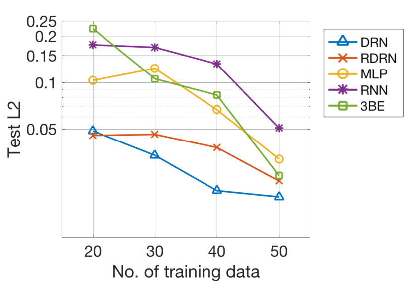
(a)

Figure 2: (a) Regression results for the shifting Gaussian and climate model datasets. $N_{p}$: number of model parameters. The number in the parentheses is the standard error over repeated runs. (b) Shifting Gaussian dataset: The test performance at small training sizes. Best viewed incolor.

5.1 Shifting Gaussian

For the first experiment, we adapted the shifting Gaussian experiment from Lampert (2015) but made it more challenging. Although this is a synthetic data set, this is the most challenging of all our datasets as it involves complex shifts in the distribution peaks. It is used to empirically study how DRN performs better even with fewer number of parameters as compared to the benchmark methods. Our shifting Gaussian means varies sinusoidally over time. Given a few consecutive input distributions taken from time steps spaced $\Delta t=0.2$ apart, we predict the next time step distribution. Because of the sinusoidal variation, it is apparent that we require more than one time step of past distributions to predict the future distribution. The specific details of the data construction is in supplementary material. We found that for all methods, a history length of 3 time steps is optimal. Following Oliva et al. (2014) the regression performance is measured by the $L_{2}$ loss, where lower $L_{2}$ loss is favorable.

The plots in Figure 2(a) show the test $L_{2}$ loss as the number of training data varies. Across the varying training sizes, DRN and RDRN outperform the other methods, except at training size of 50, where 3BE’s test performance catches up. As training size decreases, MLP, RNN and 3BE show larger decrease in test performance. DRN performs better than RDRN, except at the smallest training size of 20 where there is no significant difference. The table in Figure 1(a) shows the regression results for the training size of 20, and we note DRN and RDRN use much fewer parameters than the other methods. Overall, DRN and RDRN require at least two times fewer training data than the other methods for similar test accuracies.

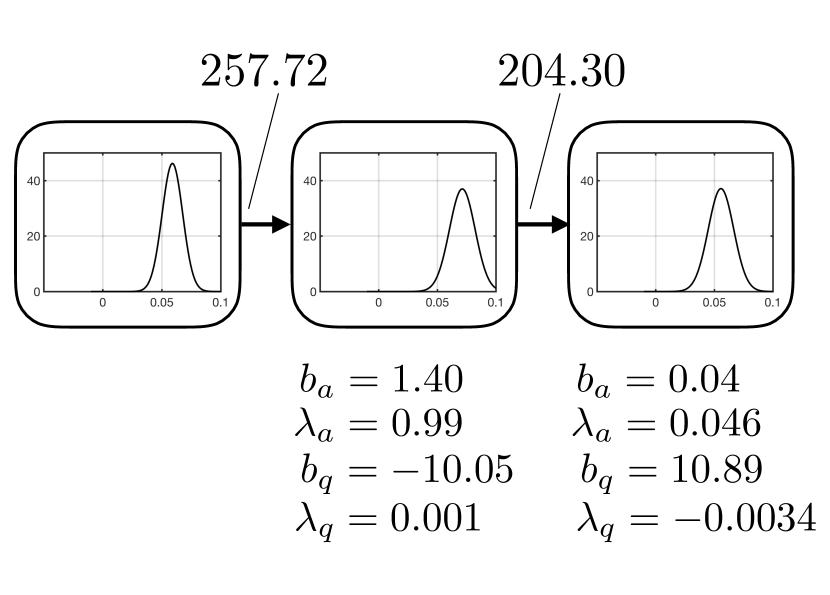
(a)

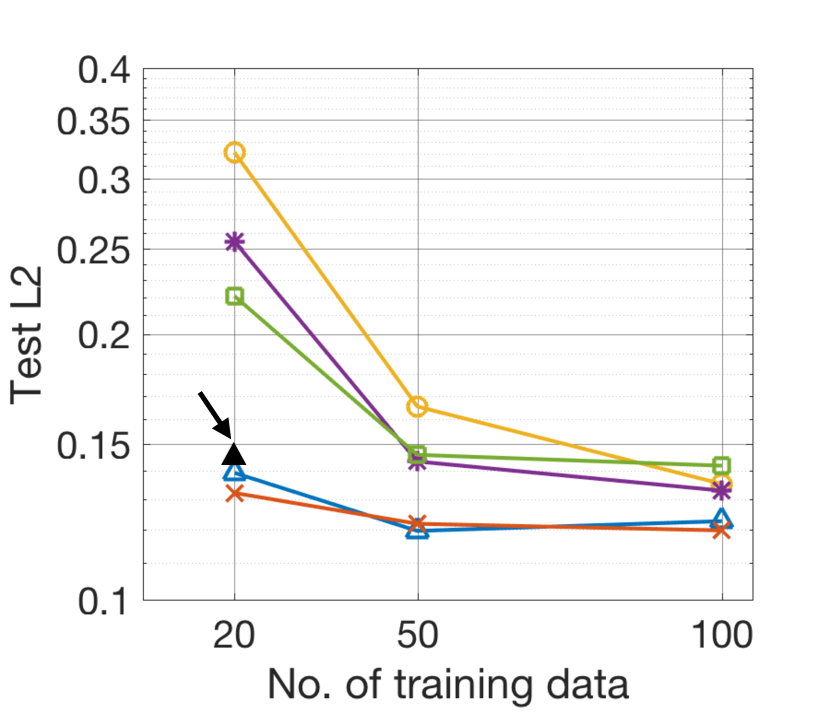
(b) Varying number of training data
(full pdf, without sampling)

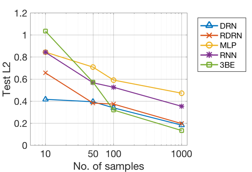
(c) Varying number of samples per distribution
(100 training data)

Figure 3: Climate model dataset: (a) A DRN network with only 2 weight and 8 bias parameters performs well for the climate model dataset. (b) The accuracies of DRN and RDRN remain high as number of training data decreases. The black triangle indicated by the arrow gives the performance obtained by the DRN network in (a). (c) As number of samples decreases, DRN and RDRN remain robust while the other methods saw larger decrease in accuracy.

5.2 Climate model

In this experiment, we test the ability of the regression methods to model unimodal Gaussian distributions spreading and drifting over time. We use a climate model which predicts how heat flux at the sea surface varies (Lin & Koshyk, 1987). The evolution of the heat flux obeys the Ornstein-Uhlenbeck (OU) process which describes how a unimodal Gaussian distribution spreads and drifts over time. The regression task is as follows: Given a sequence of distributions spaced equally apart with some fixed time gap, predict the distribution some fixed time step after the final distribution. Details of the dataset is in the supplementary material.

The regression results on the test set are shown in the table in Figure 1(a). The regression accuracies for DRN and RDRN are the best, followed by MLP and RNN. With limited training data, the performance of DRN and RDRN remain very good whereas the other methods saw large decrease in performance (see Figure  3(b)). Next, we study how the sampling noise in data affects the regression models’ performance by generating different numbers of samples drawn from distribution. Figure 3(c) shows the performance for varying number of samples drawn for a training size of 100. DRN and RDRN remain robust at large sampling noise whereas the other methods saw larger increase in error.

DRN’s compact representation of distributions allows it to perform transformations with very few network parameters, as discussed in Section 4. In Figure 3(a), we show a DRN network that has good test accuracy on the climate model dataset. The network consists of just one hidden node in between the input and output nodes and has only 10 parameters. We observe that the output distribution follows the expected behavior for the climate model: shifting towards the long-term mean at zero, with some spread from the input distribution. The DRN network in Figure 3(a) does this by first shifting the distribution right, and then left, with additional spread at each step.

	CarEvolution (5 training data)
	Test NLL	$N_{p}$
DRN	3.9663(2e-5)	28676
RDRN	3.9660(3e-4)	12313
MLP	3.9702(6e-4)	1.2e+7
3BE	3.9781(0.003)	1.2e+7
EDD	4.0405	64

(a)

	Stock (200 training data)
	Test NLL (1 day)	Test NLL (10 days)	$T$	$N_{p}$
DRN	-473.93(0.02)	-458.08(0.01)	1	9
RDRN	-469.47(2.43)	-459.14(0.01)	3	37
MLP	-471.00(0.04)	-457.08(0.98)	3	10300
RNN	-467.37(1.33)	-457.96(0.20)	3	4210
3BE	-464.22(0.16)	-379.43(11.8)	1	14000

(b)

Table 2: Regression results for the (a) CarEvolution and (b) stock dataset. $NLL$: negative log-likelihood, $T$: optimal number of input time steps, $N_{p}$: number of model parameters used. Lower loss values reflect better regression accuracies.

5.3 CarEvolution data

For the next experiment, we use the CarEvolution dataset (Rematas et al., 2013) which was used by Lampert (2015) to evaluate EDD’s ability to track the distribution drift of image datasets. This is very useful for training classifiers where the data distribution changes over time. The dataset consists of images of cars manufactured from different years and from each time period, we obtain a distribution of DeCAF features (Donahue et al., 2014) of the car images in that period. Here we make the approximation that the DeCAF features are independent. For this dataset, the distributions can be multimodal and non-Gaussian, as shown in the pdfs in the supplementary material.

The regression task is to predict the next time step distribution of features given the previous $T$ time step distributions. We found $T$=2 to work best for all methods. The regression performance is measured by the negative log-likelihood (NLL) of the test samples following Oliva et al. (2013), where lower NLL is favorable. The regression results are shown in Table 2(a). DRN and RDRN have the best test performance. RNN had difficulty in optimization possibly due to the high number of input dimensions, so the results are not presented. EDD has the fewest number of parameters as it assumes the dynamics of the distribution follows a linear mapping between the RKHS features of consecutive time steps (i.e. $T$=1). However, as the results show, the EDD model may be too restrictive for this dataset. For this dataset, since the number of training data is very small, we do not vary the size of the training set. We also do not vary the sample size since each distribution contains varying number of samples.

5.4 Stock prediction

The next experiment is on stock price distribution prediction which has been studied extensively by Kou et al. (2018). We adopt a similar experimental setup and extend to multiple time steps. Predicting future stock returns distributions has significant value in the real-world setting and here we test the methods’ abilities to perform such a task. Our regression task is as follows: given the past $T$ days’ distribution of returns of constituent companies in FTSE, Dow and Nikkei, predict the distribution of returns for constituent companies in FTSE $k$ days later. We used 5 years of daily returns and each distribution is obtained using kernel density estimation with the constituent companies’ returns as samples. In the supplementary material, we show some samples of the distributions.

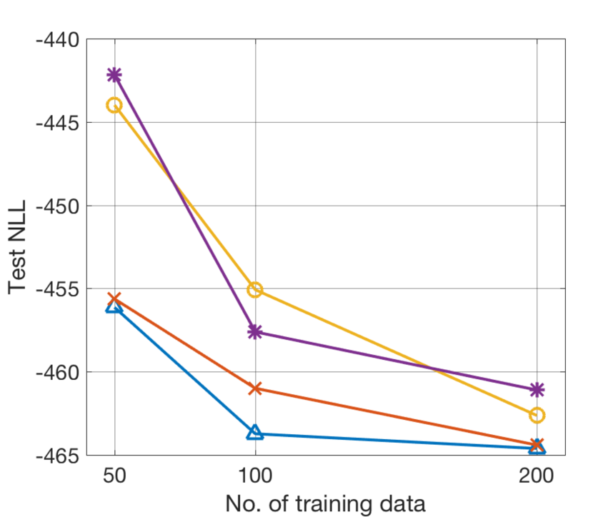
(a) 5 days ahead

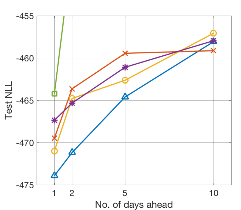
(b) 200 training data

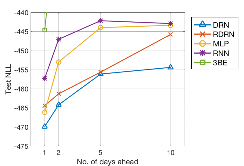
(c) 50 training data

Figure 4: Stock dataset: (a) Test negative log-likelihood for varying number of training data, for 5 days ahead prediction. DRN and RDRN’s performance remains robust at low training sizes. 3BE’s result is not shown as it is out of range. (b, c) Test NLL for varying number of days ahead prediction, for 50 and 200 training data. 3BE’s NLL is out of range for 2, 5, and 10 days ahead. DRN’s performance remains robust as number of days increases, especially for limited training size of 50.

We first observe how robust the methods are when training data is limited. Figure 4(a) shows the performance for 5 days ahead prediction with varying number of training sizes. DRN and RDRN’s performance remains robust even as the number of training data decreases from 200 to 50, whereas MLP, RNN and 3BE have larger decrease in test accuracy. Next, to study how the models perform with increasing level of task difficulty, we vary number of days ahead to predict. The results are shown in Figure 4(b) and 4(c) for 200 and 50 training data respectively. As expected, as the number of days ahead increases, the task difficulty increases and all methods see a decrease in accuracy. DRN remains robust as the number of days ahead increases, especially for the smaller training size of 50.

Table 2(b) shows the regression results for training size of 200 for 1 and 10 days ahead. For 1 day ahead performance, DRN outperforms the other methods, followed by MLP then RDRN. Since for this experiment DRN uses only one previous day of input, this suggests that the 1 day ahead prediction task does not involve long time dependencies. Predicting 10 days ahead is a more challenging task which may benefit from having a longer history of stock movements. For a training size of 200, RDRN is the best method, using 3 days of input history. This suggests that for a prediction task which involves longer time dependencies, having a recurrent architecture for DRN is beneficial when training size is sufficiently large.

6 Discussion

In this work, we address a gap in current work on distribution regression models, in that there is a lack of systematic study on the theoretical basis and generalization abilities of the various methods. The distribution regression network (DRN) has been shown to achieve higher accuracies than conventional neural networks (Kou et al., 2018). To address a lack of theoretical comparison of previous works, we studied the mathematical properties of DRN and conventional neural networks in Section 4, which gave further insights to the difference in the effects of the network parameters in the various models. In summary, we analyzed that a single weight parameter in DRN can control the propagation behavior in single nodes, ranging from the identity function to peak spreading. The propagation in DRN is highly regularized in contrast to that in MLP and CNN where there are many more parameters. In addition, DRN can fit higher order functions exponentially quickly by adding hidden layers while keeping the network compact.

These mathematical properties of DRN give insights to our experimental findings. We conducted thorough experimental validation on the generalization performance of DRN, conventional neural network models and 3BE. DRN achieves superior test accuracies with robust performance at limited training sizes, noisy data sampling and increasing task difficulty. Furthermore, the number of model parameters in DRN is much smaller. This can be attributed to the mathematical properties of DRN: the highly regularized propagation allows it to generalize better than conventional neural networks.

For future work, we look to extend to multivariate distributions, which will be useful in various applications such as modeling the 3D distribution of dark matter (Ravanbakhsh et al., 2016) and studying human populations through multi-dimensional census data (Flaxman et al., 2015). Another possibility is to extend DRN for the general function-to-function regression task.

Appendix A Recurrent extension for DRN

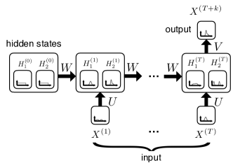
Figure 5: Recurrent distribution regression network

We introduce the recurrent distribution regression network (RDRN) which is a recurrent extension of DRN. The input data is a distribution sequence as described in Section 3.1. Figure 5 shows an example network for RDRN, where the network takes in $T$ time steps of distributions to predict the distribution at $T+k$. The hidden state at each time step may consist of multiple distributions. The arrows represent fully-connected weights. The input-hidden weights $U$ and the hidden-hidden weights $W$ are shared across the time steps. $V$ represents the weights between the final hidden state and the output distribution. The bias parameters for the hidden state nodes are also shared across the time steps. The hidden state distributions at $t=0$ represents the ‘memory’ of all past time steps before the first input and can be initialized with any prior information. In our experiments, we initialize the $t=0$ hidden states as uniform distributions as we assume no prior information is known.

We formalize the propagation for the general case where there can be multiple distributions for each time step in the data input layer and the hidden layer. Let $n$ and $m$ be the number of distributions per time step in the data layer and hidden layers respectively. Propagation starts from $t$=1 and performed through the time steps to obtain the hidden state distributions. $X_{i}^{(t)}(r_{i}^{(t)})$ represents the input data distribution at node $i$ and time step $t$, when the node variable is $r_{i}^{(t)}$. ${H}_{k}^{(t)}(s_{k}^{(t)})$ represents the density of the pdf of the $k^{\text{th}}$ hidden node at time step $t$ when the node variable is $s_{k}^{(t)}$. $\tilde{H}_{k}^{(t)}(s_{k}^{(t)})$ represents the unnormalized form. The hidden state distributions at each time step is computed from the hidden state distributions from the previous time step and the input data distribution from the current time step.

$$\tilde{H}_{k}^{(t)}\left(s_{k}^{(t)}\right) =\int_{{r_{1}}^{(t)},\cdots,{r_{n}}^{(t)},{s_{1}}^{(t-1)},\cdots,{s_{m}}^{(t-1)}}\tilde{Q}\left(s_{k}^{(t)}|r_{1}^{(t)},\cdots,s_{1}^{(t-1)},\cdots\right)$$ (6)

$$\hskip 56.9055ptX_{1}^{(t)}\left(r_{1}^{(t)}\right)\cdots X_{n}^{(t)}\left(r_{n}^{(t)}\right)H_{1}^{(t-1)}\left(s_{1}^{(t-1)}\right)\cdots H_{m}^{(t-1)}\left(s_{m}^{(t-1)}\right)$$

$$\hskip 199.16928pt\,dr_{1}^{(t)}\cdots dr_{n}^{(t)}\,ds_{1}^{(t-1)}\cdots ds_{m}^{(t-1)}$$

$$\tilde{Q}(s_{k}^{(t)}|r_{1}^{(t)},\cdots,s_{1}^{(t-1)},\cdots)=e^{-E\left(s_{k}^{(t)}|r_{1}^{(t)},\cdots,s_{1}^{(t-1)},\cdots\right)}$$ (7)

The energy function is similar to the one in DRN and is given by

$$E\left(s_{k}^{(t)}|r_{1}^{(t)},\cdots,s_{1}^{(t-1)},\cdots\right) =\sum_{i}^{n}u_{ki}\left(\frac{s_{k}^{(t)}-r_{i}^{(t)}}{\Delta}\right)^{2}+\sum_{j}^{m}w_{kj}\left(\frac{s_{k}^{(t)}-s_{j}^{(t-1)}}{\Delta}\right)^{2}$$ (8)

$$+b_{q,k}\left(\frac{s_{k}^{(t)}-\lambda_{q,k}}{\Delta}\right)^{2}+b_{a,k}\left|\frac{s_{k}^{(t)}-\lambda_{a,k}}{\Delta}\right|,$$

where for each time step, $u_{ki}$ is the weight connecting the $i^{\text{th}}$ input distribution to the $k^{\text{th}}$ hidden node. Similarly, for the hidden-hidden connections, $w_{kj}$ is the weight connecting the $j^{\text{th}}$ hidden node in the previous time step to the $k^{\text{th}}$ hidden node in the current time step. As in DRN, the hidden node distributions are normalized before propagating to the next time step. At the final time step, the output distribution is computed from the hidden state distributions, through the weight vector $V$ and bias parameters at the output node.

Appendix B Proofs for propositions for DRN theory

Forward propagation in DRN can be written as a combination of linear transformation and Hadamard products and then normalized. For a node of order $n$, its activation $p_{0}$ is

$$\tilde{p}_{0}=B_{0}\circ(T_{w_{1}}\cdot p_{1})\circ(T_{w_{2}}\cdot p_{2})\circ\cdots\circ(T_{w_{n}}\cdot p_{n})=B_{0}\circ\breve{\prod}^{n}_{i=1}T_{w_{i}}\cdot p_{i}$$ (9)

$\breve{\prod}$ is a symbol for Hadamard products and

$$p_{0}=\tilde{p}_{0}/|\tilde{p}_{0}|$$ (10)

$\circ$ is the element wise Hadamard product operator, $\cdot$ is the matrix multiplication operator. $B_{0}$ is a vector representing the bias term whose components are given by

$$(B_{0})_{i}=\exp\left(-b_{q}\left(\frac{s_{i}-\lambda_{q}}{\Delta}\right)^{2}-b_{a}\left|\frac{s_{i}-\lambda_{a}}{\Delta}\right|\right)$$ (11)

$T_{w_{i}}$ is a symmetric transformation matrix corresponding to the connections in DRN whose elements are given by

$$(T_{w_{i}})_{qr}=\exp\left(-w_{i}\left(\frac{s_{q}-s_{r}}{\Delta}\right)^{2}\right)$$ (12)

Proposition 5.

A node connecting to a target node with zero weight $w=0$ has no effect on the activation of the target node.

Proof.

Without loss of generality, suppose $w_{1}=0$ in Eq. (9), it is easy to show that

$$T_{w_{1}=0}\cdot p_{1}=e=(1,1,\cdots 1)^{t}$$ (13)

$e=(1,1,\cdots 1)^{t}$ is a vector with all ones. Using the identity, $u\circ e=u$ for any vector $u$, the term $T_{w_{1}}\cdot p_{1}$ drops out from Eq. (9). Therefore $\tilde{p}_{0}$ does not depend on $p_{1}$. ∎

Similar to conventional neural networks, this is a mechanism for which DRN can learn to ignore spurious nodes by setting their weights to zero or near zero.

Proposition 6.

For a node connecting to a target node with sufficiently large positive weight $w\to\infty$, the transformation matrix approaches the identity matrix: $T_{w}\to I$.

Proof.

Suppose $w\to\infty$ in Eq. (9), it is easy to show that

$$T_{w_{1}\to\infty}\cdot p_{1}=I\cdot p_{1}=p_{1}$$ (14)

∎

The consequence is that the identity mapping from one node to another can be realized.

Lemma 2.

Output of DRN is invariant to scaling the input by constant factors.

Proof.

Activation of one layer is invariant to scaling of the activation in the previous layer. Using Eq. (9), performing the transformation $p_{i}\leftarrow c_{i}p_{i}$, where $c_{i}$ are scalars, leads to $\tilde{p}_{0}\leftarrow c_{1}c_{2}\cdots c_{n}\tilde{p}_{0}$, subsequent normalization makes $p_{0}$ invariant to any scaling factors. The effects of scaling in a layer in the network is immediately eliminated in the next layer by normalization. ∎

Proposition 7.

Output of DRN is invariant to normalization of all hidden layers of DRN.

Proof.

For the purpose of proving, construct two networks identical in architecture and weights, forward propagate both networks, one network with nodes in the hidden layer normalized and the other network with nodes in the hidden layer unnormalized.

Let $n_{0}$ be the number of input nodes and $n_{1},\cdots$ be the number of hidden nodes in the hidden layers. Let activation in the input nodes be $p_{i}$, $i=1,\cdots n_{0}$. Let activation of the $i$th node in the $l$th hidden layer be $hn^{(l)}_{i}$ for the network with normalized hidden nodes and $hu^{(l)}_{i}$ for the network with unnormalized hidden nodes.

Performing forward propagation for both networks,

$$\tilde{hn}^{(1)}_{i}=B_{i}^{(1)}\circ\breve{\prod}_{j=1}^{n_{0}}T_{w^{(1)}_{j}}\cdot p_{j}$$ (15)

$${hn}^{(1)}_{i}=\frac{\tilde{hn}^{(1)}_{i}}{|\tilde{hn}^{(1)}_{i}|}$$ (16)

$$\tilde{hu}^{(1)}_{i}=B_{i}^{(1)}\circ\breve{\prod}_{j=1}^{n_{0}}T_{w^{(1)}_{j}}\cdot p_{j}=\tilde{hn}^{(1)}_{i}$$ (17)

For the second layer,

$$\tilde{hn}^{(2)}_{i} = B_{i}^{(2)}\circ\breve{\prod}_{j=1}^{n_{1}}T_{w^{(2)}_{j}}\cdot hn^{(1)}_{j}$$ (18)

$$= \frac{B_{i}^{(2)}\circ\breve{\prod}_{j=1}^{n_{1}}T_{w^{(2)}_{j}}\cdot\tilde{hn}^{(1)}_{j}}{\prod_{j^{\prime}=1}^{n_{1}}|\tilde{hn}^{(1)}_{j^{\prime}}|}$$

$$= \frac{B_{i}^{(2)}\circ\breve{\prod}_{j=1}^{n_{1}}T_{w^{(2)}_{j}}\cdot\tilde{hn}^{(1)}_{j}}{z^{(1)}}$$

$z^{(1)}=\prod_{j^{\prime}=1}^{n_{1}}|\tilde{hn}^{(1)}_{j^{\prime}}|$ is the normalization scalar that factorizes out of the Hadamard product.

$${hn}^{(2)}_{i}=\frac{\tilde{hn}^{(2)}_{i}}{|\tilde{hn}^{(2)}_{i}|}$$ (20)

$$\tilde{hu}^{(2)}_{i} = B_{i}^{(2)}\circ\breve{\prod}_{j=1}^{n_{1}}T_{w^{(2)}_{j}}\cdot\tilde{hu}^{(1)}_{j}$$

$$\tilde{hu}^{(2)}_{i} = \tilde{hn}^{(2)}_{i}z^{(1)}$$ (21)

Using Eq. (21), it can be shown that,

$$\tilde{hu}^{(l)}_{i}=\tilde{hn}^{(l)}_{i}\prod^{(l-1)}_{j=1}z^{(j)}=\tilde{hn}^{(l)}_{i}Z^{(l-1)}$$ (22)

Without loss of generality, assume that the output consists of one node, let $pn$ and $pu$ be the final normalized output of the networks with normalized hidden layers and unnormalized hidden layers respectively. Using Eq. (22), we shall proof that $pn=pu$.

$$\tilde{pn} = (B^{(L)})\circ\breve{\prod}_{j=1}^{n_{L-1}}(T_{w_{j}^{(L)}}\cdot hn^{(L-1)}_{j})$$ (23)

$$\tilde{pu} = (B^{(L)})\circ\breve{\prod}_{j=1}^{n_{L-1}}(T_{w_{j}^{(L)}}\cdot\tilde{hu}^{(L-1)}_{j})$$ (24)

$$= (B^{(L)})\circ\breve{\prod}_{j=1}^{n_{L-1}}(T_{w_{j}^{(L)}}\cdot\tilde{hn}^{(L-1)}_{j})Z^{(L-1)}$$

Eq. (23) and (24) show that $\tilde{pn}$ and $\tilde{pu}$ differ by a constant scalar. Therefore, after normalizing, $pn=pu$. ∎

Although normalization is theoretically unnecessary, normalization step in Eq. (10) provides numerical stability and prevents numeric under-flows and over-flows.

Definition 2.

A node in DRN is said to be an order $n$ node when it is connected with non-zero weights from $n$ incoming nodes in the previous layer.

Lemma 3.

For an order $n$ node, components of $\tilde{p}_{0}$ (which we denote as $\tilde{p}_{0i}$, where $i=1,\cdots,q$ and $q$ is the distribution discretization size), follow a power law of $n$th order cross terms of the components of connecting nodes.

Proof.

By rearranging the cross terms in the Hadamard product, we obtain the $n$th order cross terms from the components of the connecting nodes.

$$\tilde{p}_{0i} = {(B_{0})}_{i}\left(\sum_{j_{1}}(T_{w_{1}})_{i,j_{1}}(p_{1})_{j_{1}}\right)\cdots\left(\sum_{j_{n}}(T_{w_{n}})_{i,j_{n}}(p_{1})_{j_{n}}\right)$$ (25)

$$= (B_{0})_{i}\sum_{j_{1}}\cdots\sum_{j_{n}}\underbrace{\left[(T_{w_{1}})_{i,j_{1}}\cdots(T_{w_{n}})_{i,j_{n}}\right]}_{\text{coefficients}}\underbrace{\left[(p_{1})_{j_{1}}\cdots(p_{n})_{j_{n}}\right]}_{\text{cross terms}}$$

∎

Writing in short hand notation, $J^{(1)}=(j_{1},\cdots j_{n})$ where the superscript indicates $J$ is the indices over the first layer. Write $\sum_{j_{1}}\cdots\sum_{j_{n}}=\sum_{J^{(1)}}$ and consolidate the coefficients into a tensor, $c_{i,J^{(1)}}(w,B)=(B_{0})_{i}(T_{w_{1}})_{i,j_{1}}\cdots(T_{w_{n}})_{i,j_{n}}$, and the cross terms into a tensor, $P_{J^{(1)}}=(p_{1})_{j_{1}}\cdots(p_{n})_{j_{n}}$, where $w=(w_{1},\cdots w_{n})$. Eq. (25) can be written compactly as,

$$\tilde{p}_{0i}=\sum_{J^{(1)}}c_{i,J^{(1)}}(w,B)P_{J^{(1)}}$$ (26)

The normalization factor is,

$$|\tilde{p}_{0}|=\sum_{J^{(1)}}\sum_{i}c_{i,J^{(1)}}(w,B)P_{J^{(1)}}=\sum_{J^{(1)}}z_{J^{(1)}}P_{J^{(1)}}$$ (27)

Finally, the normalized output, written in vector notation is,

$$p_{0}=\frac{\sum_{J^{(1)}}c_{J^{(1)}}P_{J^{(1)}}}{\sum_{{\hat{J}}^{(1)}}z_{{\hat{J}}^{(1)}}P_{{\hat{J}}^{(1)}}}$$ (28)

where $p_{0}=(p_{01},p_{02},\cdots p_{0q})$ and $c_{J^{(1)}}=(c_{1,J^{(1)}},\cdots c_{q,J^{(1)}})$.

For a network with hidden layers, let $h^{(l)}_{1},\cdots h^{(l)}_{n_{l}}$ be the activation in the $l$th hidden layer. By Proposition 7, we only consider unnormalized hidden layers. The activation on the first hidden layer can be written using Eq. (28) without the normalization factor. Using $J^{(1)}_{\alpha}$ to denote the indices connecting to $h^{(1)}_{\alpha}$,

$$h^{(1)}_{\alpha}=\sum_{J^{(1)}_{\alpha}}c_{J^{(1)}_{\alpha}}(w^{(1)}_{\alpha},B^{(1)}_{\alpha})P_{J^{(1)}_{\alpha}}$$ (29)

For the nodes in the second hidden layer, $h^{(2)}_{\alpha}$,

$$h^{(2)}_{\alpha}=\sum_{J^{(2)}_{\alpha}}c_{J^{(2)}_{\alpha}}(w^{(2)}_{\alpha},B^{(2)}_{\alpha})H_{J^{(2)}_{\alpha}}$$ (30)

$$H_{J^{(2)}_{\alpha}} = (h^{(1)}_{1})_{j_{1}}(h^{(1)}_{2})_{j_{2}}\cdots(h^{(1)}_{n_{1}})_{j_{n_{1}}}$$ (31)

$$= \left(\sum_{J^{(1)}_{1}}c_{j_{1},J^{(1)}_{1}}P_{J^{(1)}_{1}}\right)\cdots\left(\sum_{J^{(1)}_{n_{1}}}c_{j_{n_{1}},J^{(1)}_{n_{1}}}P_{J^{(1)}_{n_{1}}}\right)$$

$$= \prod_{\beta=1}^{n_{1}}\left(\sum_{J^{(1)}_{\beta}}c_{j_{\beta},J^{(1)}_{\beta}}P_{J^{(1)}_{\beta}}\right)$$

Each of the $P_{J^{(1)}_{\beta}}$ consists of cross terms of the input distributions to order $n_{0}$ ($n_{0}$ is the number of input nodes). $H_{J^{(2)}_{\alpha}}$ is a product of $n_{1}$ $P_{J^{(1)}_{\beta}}$’s, hence $H_{J^{(2)}_{\alpha}}$ will be cross terms of the input distributions to order $n_{1}\times n_{0}$.

For a network of $L$ hidden layers with number of nodes, $n_{1},n_{2},\cdots n_{L}$, the output consist of multiplications of the components of input distributions to the power of $n_{0}\times n_{1}\cdots\times n_{L}$. In this way, DRN can fit high order functions exponentially quickly by adding hidden layers.

Proposition 8.

For a node of order $n$, in the limit of small weights $|w_{\alpha}|\ll 1$ for $\alpha=1,\cdots n$, the output activions, ${p}_{0}$ can be approximated as a fraction of two linear combinations of the activations in the input nodes.

Proof.

In the limit of small weights, one can expand $T_{w_{\alpha}}$ and keep the terms linear in $w_{\alpha}$. Then $T_{w_{\alpha}}$ is of the form

$$T_{w_{\alpha}} = E+\mathcal{E}_{w_{\alpha}}+\mathcal{O}(w_{\alpha}^{2})$$ (32)

where $E$ is a matrix with all ones in its elements, $\mathcal{O}(w_{\alpha}^{2})$ is a matrix with elements of the order of $w_{\alpha}^{2}$ and $\mathcal{E}_{w_{\alpha}}$ is a matrix linear in $w_{\alpha}$ given by,

$$\mathcal{E}_{w_{\alpha}}=\left(\begin{array}[]{ccc}0&-w_{\alpha}/\Delta^{2}&-4w_{\alpha}/\Delta^{2}\cdots\\ -w_{\alpha}/\Delta^{2}&0&-w_{\alpha}/\Delta^{2}\cdots\\ \vdots&&\end{array}\right)$$ (33)

Using Eq.(9) and dropping higher order terms,

$$\tilde{p}_{0}\approx B_{0}\circ((E+\mathcal{E}(w_{1}))\cdot p_{1})\circ((E+\mathcal{E}(w_{2}))\cdot p_{2})\circ\cdots\circ((E+\mathcal{E}(w_{n}))\cdot p_{n})\\$$

Expanding and using the distributive property of Hadamard product (Million, 2007), then dropping higher order terms in $w_{i}$ again,

$$\tilde{p}_{0i}\approx B_{0i}+\sum_{\alpha}B_{0i}\circ(\mathcal{E}(w_{\alpha})\cdot p_{\alpha})_{i}$$ (34)

Upon normalization,

$$p_{0i}\approx\frac{B_{0i}+\sum_{\alpha}B_{0i}\circ(\mathcal{E}(w_{\alpha})\cdot p_{\alpha})_{i}}{\sum_{j}\left[B_{0j}+\sum_{\alpha^{\prime}}B_{0j}\circ(\mathcal{E}(w_{\alpha^{\prime}})\cdot p_{\alpha^{\prime}})_{j}\right]}$$ (35)

∎

The consequence of proposition 8 is that by adjusting the weights, DRN can approximate the unnormalized output distribution to be a fraction of linear combinations of the input distribution.

Indeed, the matrix $T_{w_{\alpha}}$ can be approximated by expanding to $K$ orders in $w_{\alpha}$ with accuracy of expansion depending on the magnitudes of $w_{\alpha}$. If expansion is up to second order in $w_{\alpha}$ then the output is a fraction of quadratic expressions. If the expansion in $w_{\alpha}$ is up to $K$ order then the resulting output is a fraction of polynomials of $K$ order. At this point we wish to mention DRN’s analogy to the well known Padé approximant (Baker et al., 1996). Padé approximant is a method of function approximation using fraction of polynomials.

Appendix C Experimental details

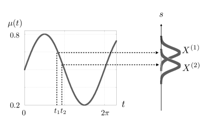
Figure 6:

C.1 Shifting Gaussian

We track a Gaussian distribution whose mean varies in the range $[0.2,0.8]$ sinusoidally over time while the variance is kept constant at 0.1 (see Figure 6). Given a few consecutive input distributions taken from time steps spaced $\Delta t=0.2$ apart, we predict the next time step distribution. For each data we randomly sample the first time step from $[0,2\pi]$. The distributions are truncated with support of $[0,1]$ and discretized with $q$=100 bins. We found that for all methods, a history length of 3 time steps is optimal. Following Oliva et al. (2014) the regression performance is measured by the $L_{2}$ loss, where lower $L_{2}$ loss is favorable. Table 3 shows the detailed network architectures used, for training size of 20. $q=100$ was used for the discretization of the distributions.

Comparison of models tuned for best validation set result (Shifting Gaussian dataset, 20 training data) Test $L_{2}(10^{-2})$ $T$ Model description $N_{p}$ Cost function DRN 4.90(0.46) 3 3 - 2x10 - 1 224 JS divergence RDRN 4.55(0.42) 3 T = 3, m = 5 59 JS divergence MLP 10.32(0.41) 3 300 - 1x3 - 100 1303 MSE RNN 17.50(0.89) 3 T = 3, m = 10 2210 MSE 3BE 22.30(1.89) 3 30 basis functions, 20k RKS features 6e+5 $L_{2}$ loss

Table 3: Regression resutls for the shifting Gaussian dataset, with descriptions of the models. $L_{2}$ denotes the $L_{2}$ loss, $T$ is the optimal number of input time steps and $N_{p}$ is the number of model parameters used, MSE represents the mean squared error. A discretization of $q=100$ is used for the distributions. For RDRN and RNN, $m$ is the number of nodes in the hidden state of each time step. For DRN and MLP (feedforward networks), the architecture is denoted as such: Eg. 3 - 2x10 - 1: 3 input nodes, with 2 fully-connected hidden layers each with 10 nodes, and 1 output node.

C.2 Climate Model

With the long-term mean set at zero, the pdf has a mean of $\mu(t)=y\exp(-\theta t)$ and variance of $\sigma^{2}(t)=D(1-e^{-2\theta t})/\theta$. $t$ represents time, $y$ is the initial point mass position, and $D$ and $\theta$ are the diffusion and drift coefficients respectively. The diffusion and drift coefficients are determined from real data measurements Oort & Rasmusson (1971): $D=0.0013,$ $\theta=2.86$, and each unit of time corresponds to 55 days (Lin & Koshyk, 1987). To create a distribution sequence, we first sample $y\in[0.02,0.09]$. For each $y$, we generate 6 Gaussian distributions at $t_{0}-4\delta$, $t_{0}-3\delta$, …, $t_{0}$ and $t_{0}+0.02$, with $\delta=0.001$ and $t_{0}$ sampled uniformly from $[0.01,0.05]$. The Gaussian distributions are truncated with support of $[-0.01,0.1]$. The regression task is as follows: Given the distributions at $t_{0}-4\delta$, $t_{0}-3\delta$, …, $t_{0}$, predict the distribution at $t_{0}+0.02$. With different sampled values for $y$ and $t_{0}$, we created 100 training and 1000 test data. Table 4 shows the detailed network architectures used, for training size of 100. $q=100$ was used for the discretization of the distributions.

Comparison of models tuned for best validation set result (Climate model dataset, 100 training data) Test $L_{2}(10^{-2})$ $T$ Model description $N_{p}$ Cost function DRN 12.27(0.34) 3 3 - 1x5 - 1 44 JS divergence RDRN 11.98(0.13) 5 T = 5, m = 5 59 JS divergence MLP 13.52(0.25) 3 300 - 2x50 - 100 22700 MSE RNN 13.29(0.59) 5 T = 5, m = 50 12650 MSE 3BE 14.18(1.29) 5 11 basis functions, 20k RKS features 2.2e+5 $L_{2}$ loss

Table 4: Regression results for the climate model dataset, with descriptions of the models. $L_{2}$ denotes the $L_{2}$ loss, $T$ is the optimal number of input time steps and $N_{p}$ is the number of model parameters used, MSE represents the mean squared error. A discretization of $q=100$ is used for the distributions. For RDRN and RNN, $m$ is the number of nodes in the hidden state of each time step. For DRN and MLP (feedforward networks), the architecture is denoted as such: Eg. 3 - 2x10 - 1: 3 input nodes, with 2 fully-connected hidden layers each with 10 nodes, and 1 output node.

C.3 CarEvolution data

The dataset consists of 1086 images of cars manufactured from the years 1972 to 2013. We split the data into intervals of 5 years (i.e. 1970-1975, 1975-1980, $\cdots$, 2010-2015) where each interval has an average of 120 images. This gives 9 time intervals and for each interval, we create the data distribution from the DeCAF (fc6) features (Donahue et al., 2014) of the car images using kernel density estimation. The DeCAF features have 4096 dimensions. Performing accurate density estimation in very high dimensions is challenging due to the curse of dimensionality (Gu et al., 2013). Here we make the approximation that the DeCAF features are independent, such that the joint probability is a product of the individual dimension probabilities. The first 7 intervals were used for the train set while the last 3 intervals were used for the test set, giving 5 training and 1 test data. Table 5 shows the detailed network architectures used for the CarEvolution dataset, for training size of 5. $q=100$ was used for the discretization of the distributions. Figure 7 shows some samples of the distributions formed from the CarEvolution dataset. The distributions’ shapes are much more varied than simple Gaussian distributions.

Table 5: Regression results for the CarEvolution dataset, with descriptions of the models. NLL denotes the negative log-likelihood, $T$ is the optimal number of input time steps and $N_{p}$ is the number of model parameters used, MSE represents the mean squared error. A discretization of $q=100$ is used for the distributions. For RDRN and RNN, $m$ is the number of nodes in the hidden state of each time step. For DRN and MLP (feedforward networks), the architecture is denoted as such: Eg. 3 - 2x10 - 1: 3 input nodes, with 2 fully-connected hidden layers each with 10 nodes, and 1 output node.

Comparison of models tuned for best validation set result (CarEvolution dataset, 5 training data) Test NLL $T$ Model description $N_{p}$ Cost function DRN 3.9663(2e-5) 2 (4096x2) - 1x1 - 4096 28676 JS divergence RDRN 3.9660(3e-4) 2 T = 2, m = 3 12313 JS divergence MLP 3.9702(6e-4) 2 (4096x2x100) - 3x10 - (4096x100) 1.2e+7 MSE 3BE 3.9781(0.003) 2 15 basis functions, 200 RKS features 1.2e+7 $L_{2}$ loss EDD 4.0405 1 8x8 kernel matrix for 8 training data 64 MSE

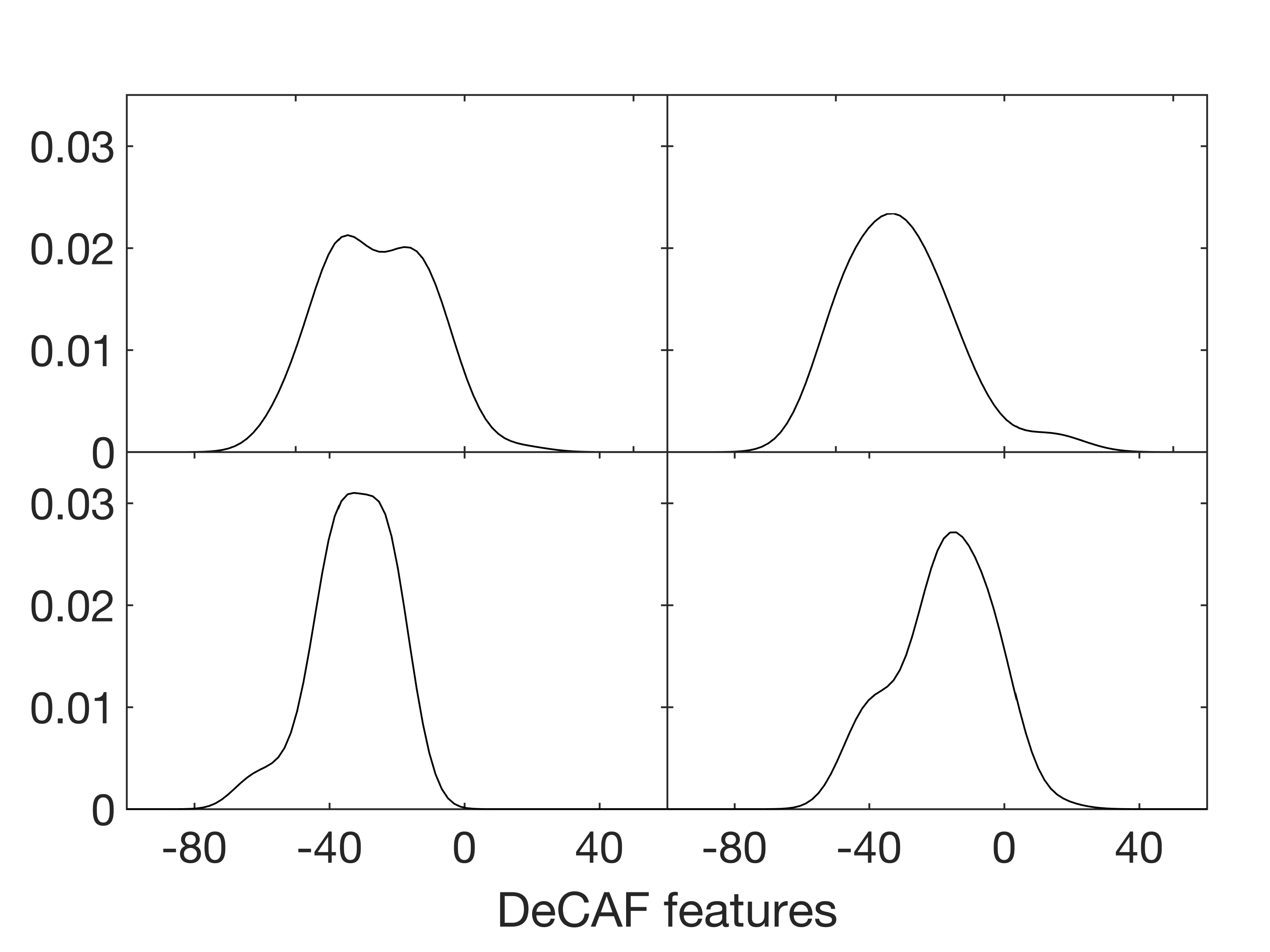
Figure 7: Samples of the DeCAF features (Donahue et al., 2014) distributions for the CarEvolution dataset, showing varied distribution shapes.

C.4 Stock prediction

We used 5 years of daily returns from 2011 to 2015 and performed exponential window averaging on the price series (Murphy, 1999). We also used a sliding-window training scheme (Kaastra & Boyd, 1996) to account for changing market conditions (details are in C.4). The daily stock returns are the logarithmic returns. We used a sliding window scheme where a new window is created and the model retained after every 300 days (the size of the test set). For each window, the previous 500 and 100 days were used for training and validation sets respectively. Table 6 shows the detailed network architectures used. $q=100$ was used for the discretization of the distributions. The RDRN architecture used is shown in Figure 8, where the data input consists past 3 days of distribution returns and one layer of hidden states with 3 nodes per time step is used. Figure 9 shows some samples of the distributions formed from the stock dataset. The distribution shapes are much more varied than simple Gaussian distributions.

Table 6: Regression results for the stock dataset, with descriptions of the models. NLL denotes the negative log-likelihood, $T$ is the optimal number of input time steps and $N_{p}$ is the number of model parameters used, MSE represents the mean squared error. A discretization of $q=100$ is used for the distributions. For RDRN and RNN, $m$ is the number of nodes in the hidden state of each time step. For DRN and MLP (feedforward networks), the architecture is denoted as such: Eg. 3 - 2x10 - 1: 3 input nodes, with 2 fully-connected hidden layers each with 10 nodes, and 1 output node.

Comparison of models tuned for best validation set result (Stock dataset, 200 training data) Test NLL 1 day 10 days $T$ Model description $N_{p}$ Cost function DRN -473.93(0.02) -458.08(0.01) 1 No hidden layer 9 JS divergence RDRN -469.47(2.43) -459.14(0.01) 3 T = 3, m = 3 37 JS divergence MLP -471.00(0.04) -457.08(0.98) 3 (3x3x100) - 3x10 - 100 10300 MSE RNN -467.37(1.33) -457.96(0.20) 3 T = 3, m = 10 4210 MSE 3BE -464.22(0.16) -379.43(11.8) 1 14 basis functions, 1k RKS features 14000 $L_{2}$ loss

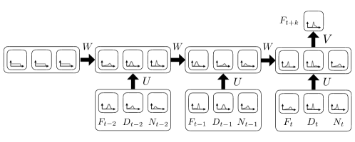
Figure 8: RDRN network for the stock dataset: past 3 days of distribution of returns of constituent companies in FTSE, DOW and Nikkei were used as inputs, to predict the future distribution of returns for constituent companies in FTSE. One layer of hidden states is used, with 3 nodes per hidden state.

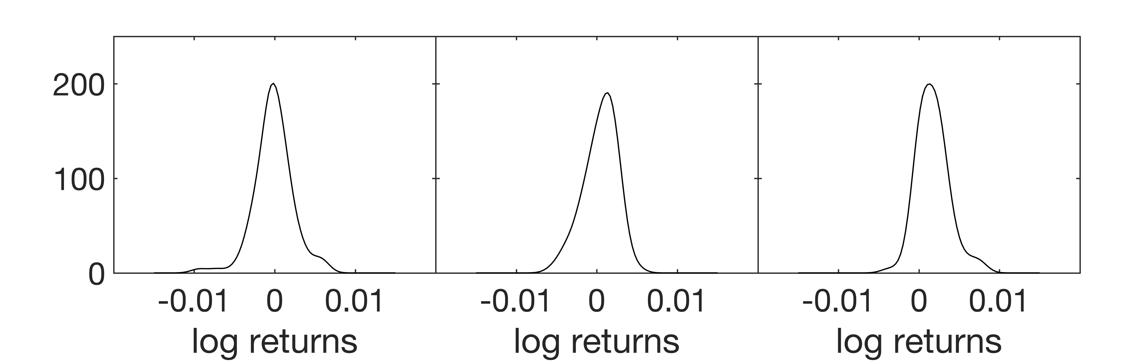
(a) FTSE

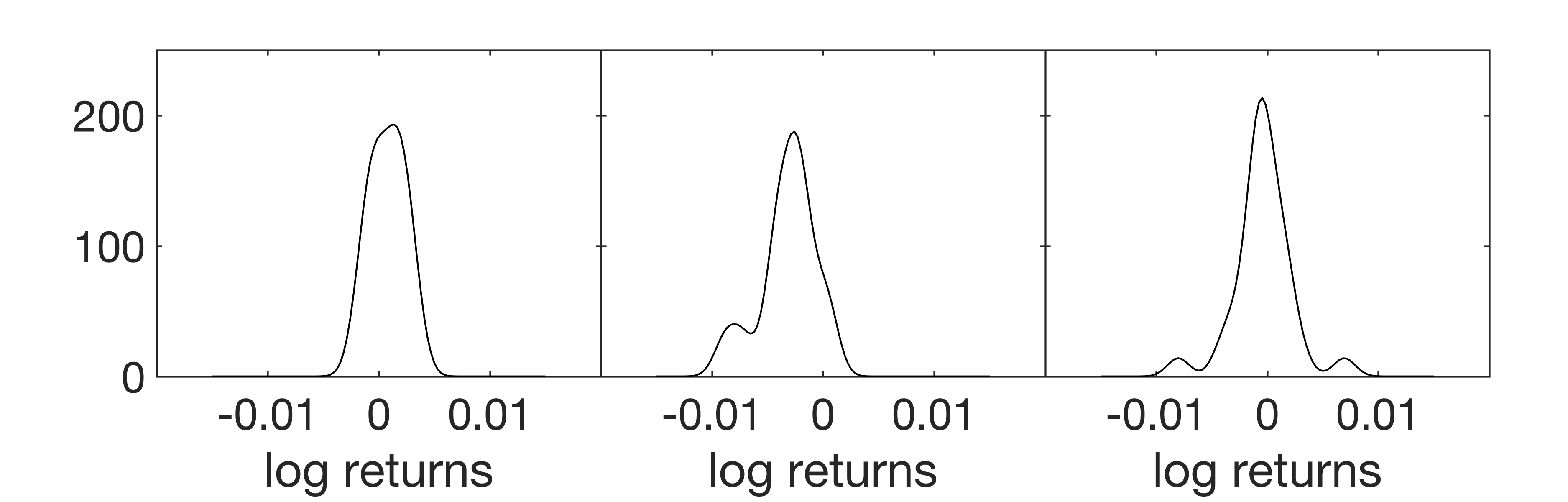
(b) DOW

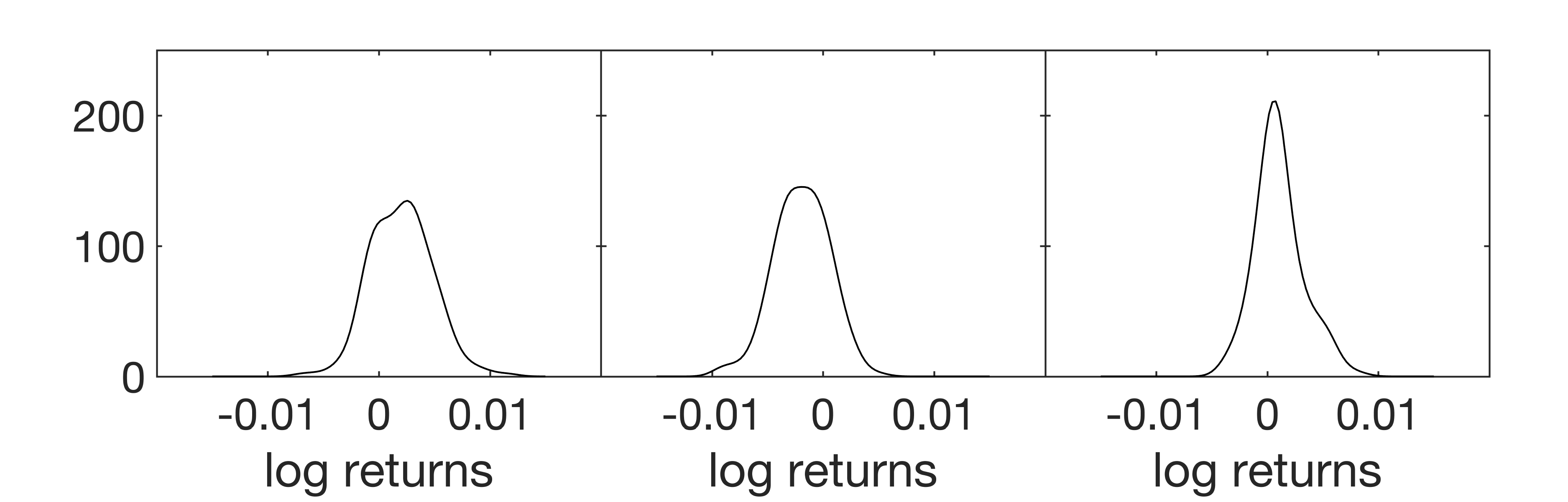
(c) Nikkei

Figure 9: Samples of the data distributions formed from (a) FTSE, (b) DOW and (c) Nikkei constitutent companies’ log returns.

References

- Baker et al. (1996) Baker, George A, Baker Jr, George A, BAKER JR, GEORGE A, Graves-Morris, Peter, and Baker, Susan S. Padé approximants, volume 59. Cambridge University Press, 1996.
- Donahue et al. (2014) Donahue, Jeff, Jia, Yangqing, Vinyals, Oriol, Hoffman, Judy, Zhang, Ning, Tzeng, Eric, and Darrell, Trevor. Decaf: A deep convolutional activation feature for generic visual recognition. In International conference on machine learning, pp. 647–655, 2014.
- Flaxman et al. (2015) Flaxman, Seth R, Wang, Yu-Xiang, and Smola, Alexander J. Who supported obama in 2012?: Ecological inference through distribution regression. In Proceedings of the 21th ACM SIGKDD International Conference on Knowledge Discovery and Data Mining, pp. 289–298. ACM, 2015.
- Gu et al. (2013) Gu, Chong, Jeon, Yongho, and Lin, Yi. Nonparametric density estimation in high-dimensions. Statistica Sinica, pp. 1131–1153, 2013.
- Guérin et al. (2011) Guérin, T, Prost, J, and Joanny, J-F. Bidirectional motion of motor assemblies and the weak-noise escape problem. Physical Review E, 84(4):041901, 2011.
- Kaastra & Boyd (1996) Kaastra, Iebeling and Boyd, Milton. Designing a neural network for forecasting financial and economic time series. Neurocomputing, 10(3):215–236, 1996.
- Katsura (1962) Katsura, Shigetoshi. Statistical mechanics of the anisotropic linear heisenberg model. Physical Review, 127(5):1508, 1962.
- Kou et al. (2018) Kou, Connie Khor Li, Lee, Hwee Kuan, and Ng, Teck Khim. A compact network learning model for distribution regression. Neural Networks, 2018. ISSN 0893-6080. doi: https://doi.org/10.1016/j.neunet.2018.12.007. URL http://www.sciencedirect.com/science/article/pii/S0893608018303381.
- Lampert (2015) Lampert, Christoph H. Predicting the future behavior of a time-varying probability distribution. In Proceedings of the IEEE Conference on Computer Vision and Pattern Recognition, pp. 942–950, 2015.
- LeCun et al. (2015) LeCun, Yann, Bengio, Yoshua, and Hinton, Geoffrey. Deep learning. nature, 521(7553):436, 2015.
- Lee et al. (2002) Lee, Hwee Kuan, Schulthess, Thomas C, Landau, David P, Brown, Gregory, Pierce, John Philip, Gai, Z, Farnan, GA, and Shen, J. Monte Carlo simulations of interacting magnetic nanoparticles. Journal of applied physics, 91(10):6926–6928, 2002.
- Lin & Koshyk (1987) Lin, Charles A and Koshyk, John N. A nonlinear stochastic low-order energy balance climate model. Climate dynamics, 2(2):101–115, 1987.
- Lin (1991) Lin, Jianhua. Divergence measures based on the Shannon entropy. IEEE Transactions on Information theory, 37(1):145–151, 1991.
- Million (2007) Million, Elizabeth. The hadamard product. Course Notes, 3:6, 2007.
- Murphy (1999) Murphy, John J. Technical analysis of the futures markets: A comprehensive guide to trading methods and applications, New York Institute of Finance, 1999.
- Noble & Wheatland (2011) Noble, PL and Wheatland, MS. Modeling the sunspot number distribution with a fokker-planck equation. The Astrophysical Journal, 732(1):5, 2011.
- Oliva et al. (2015) Oliva, Junier, Neiswanger, William, Póczos, Barnabás, Xing, Eric, Trac, Hy, Ho, Shirley, and Schneider, Jeff. Fast function to function regression. In Artificial Intelligence and Statistics, pp. 717–725, 2015.
- Oliva et al. (2013) Oliva, Junier B, Póczos, Barnabás, and Schneider, Jeff G. Distribution to distribution regression. In ICML (3), pp. 1049–1057, 2013.
- Oliva et al. (2014) Oliva, Junier B, Neiswanger, Willie, Póczos, Barnabás, Schneider, Jeff G, and Xing, Eric P. Fast distribution to real regression. In AISTATS, pp. 706–714, 2014.
- Oort & Rasmusson (1971) Oort, Abraham H and Rasmusson, Eugene M. Atmospheric circulation statistics, volume 5. US Government Printing Office, 1971.
- Palmer (2000) Palmer, Tim N. Predicting uncertainty in forecasts of weather and climate. Reports on progress in Physics, 63(2):71, 2000.
- Póczos et al. (2013) Póczos, Barnabás, Singh, Aarti, Rinaldo, Alessandro, and Wasserman, Larry A. Distribution-free distribution regression. In AISTATS, pp. 507–515, 2013.
- Ravanbakhsh et al. (2016) Ravanbakhsh, Siamak, Oliva, Junier B, Fromenteau, Sebastian, Price, Layne, Ho, Shirley, Schneider, Jeff G, and Póczos, Barnabás. Estimating cosmological parameters from the dark matter distribution. In ICML, pp. 2407–2416, 2016.
- Rematas et al. (2013) Rematas, Konstantinos, Fernando, Basura, Tommasi, Tatiana, and Tuytelaars, Tinne. Does evolution cause a domain shift? In Proceedings VisDA 2013, pp. 1–3, 2013.
- Risken (1996) Risken, Hannes. Fokker-planck equation. In The Fokker-Planck Equation, pp. 63–95. Springer, 1996.