Disk wind feedback from high-mass protostars

Abstract

We perform a sequence of 3D magnetohydrodynamic (MHD) simulations of the outflow-core interaction for a massive protostar forming via collapse of an initial cloud core of $60~{}{M_{\odot}}$. This allows us to characterize the properties of disk wind driven outflows from massive protostars, which can allow testing of different massive star formation theories. It also enables us to assess quantitatively the impact of outflow feedback on protostellar core morphology and overall star formation efficiency. We find that the opening angle of the flow increases with increasing protostellar mass, in agreement with a simple semi-analytic model. Once the protostar reaches $\sim 24~{}{M_{\odot}}$ the outflow’s opening angle is so wide that it has blown away most of the envelope, thereby nearly ending its own accretion. We thus find an overall star formation efficiency of $\sim 50\%$, similar to that expected from low-mass protostellar cores. Our simulation results therefore indicate that the MHD disk wind outflow is the dominant feedback mechanism for helping to shape the stellar initial mass function from a given prestellar core mass function.

1 Introduction

Bipolar jets and outflows are commonly observed from accretion disks around low-mass protostars (e.g., Bacciotti et al., 2000; Ray et al., 2007; Coffey et al., 2008). The launching of this outflow is thought to be due to magnetocentrifugal acceleration (Blandford & Payne, 1982; Konigl & Pudritz, 2000), in which a large-scale magnetic field threads the accretion disk. Gas can flow along the magnetic field lines if they are inclined sufficiently with respect to the disk. The gas gains speed as it flows along the field lines. Beyond the Alfvén surface, the field lines will become twisted, which collimates the flow. Although typically more difficult to observe, high-mass protostars are also often seen to have associated jets and outflows (e.g., Arce et al., 2007; Beltrán & de Wit, 2016; Hirota et al., 2017). Indeed, outflows are very commonly seen in most astrophysical settings where there is an accretion disk surrounding a central object, and the magnetocentrifugal model was first proposed for AGN jets. The disk wind mechanism has been studied extensively with numerical simulations (e.g., Shibata & Uchida, 1985; Uchida & Shibata, 1985; Ouyed & Pudritz, 1997; Romanova et al., 1997; Ouyed et al., 1997, 2003; Anderson et al., 2006; Moll, 2009; Staff et al., 2010, 2015; Ramsey & Clarke, 2011; Stute et al., 2014). Other models for launching the outflow have also been proposed. For instance, an outflow may originate in the innermost part of the disk or the disk/magnetosphere boundary (often referred to as the X-wind model, Lovelace et al., 1991; Shu et al., 2000), a stellar wind (Matt & Pudritz, 2005), or driven by the magnetic pressure of the magnetic field (i.e., magnetic tower model of Lynden-Bell, 1996).

One possible formation scenario for high-mass stars is that of Core Accretion, i.e., it is simply a scaled-up version of the standard model for low-mass star formation by accretion from gravitationally bound cores (Shu, Adams & Lizano 1987). In the Turbulent Core Model (McKee & Tan, 2002, 2003), a combination of turbulence and magnetic pressure provide most of the support in a massive core against gravity. In high pressure conditions typical of observed massive star forming regions, the accretion rate from such massive cores is expected to be relatively high, i.e., with $\sim 10^{-4}\>$ to $\sim 10^{-3}\>M_{\odot}\>{\rm yr}^{-1}$, compared to lower-mass protostars in lower pressure regions, i.e., with $\sim 10^{-6}\>$ to $\sim 10^{-5}\>M_{\odot}\>{\rm yr}^{-1}$. In this scenario, the outflows from forming massive stars may therefore also be a scaled-up version of the outflows from lower-mass stars, but with higher mass outflow rates and momentum rates. Alternative formation scenarios include models in which multiple smaller objects form close together, and then collide to form larger stars (Bonnell et al., 1998), and Competitive Accretion (Bonnell et al., 2001), in which stars forming in central, dense regions of protoclusters accrete most of their mass from a globally collapsing reservoir of ambient clump material (see Tan et al., 2014 for a review). In these models, outflows are expected to be more disordered.

There are some observations of highly collimated jets from massive young stellar objects (YSOs). For example, Marti et al. (1993) found a bipolar jet from the central source between HH 80 and 81. McLeod et al. (2018) reported observations of HH 1177, a jet originating from a massive YSO in the Large Magellanic Cloud. Caratti o Garatti et al. (2015) observed jets from 18 intermediate and high mass YSOs, and found that these jets appear as a scaled-up version of jets from lower-mass YSOs. Carrasco-González et al. (2010) and Sanna et al. (2015) studied the magnetic field morphology near massive YSOs, and found a magnetic field configuration parallel to the outflow and perpendicular to the disk. Observations of wider angle, but still collimated, molecular outflows have also been reported: see for instance Beuther et al. (2002); Wu et al. (2004); Zhang et al. (2013b, 2014a); Maud et al. (2015). The general trend found in these works is that a more luminous (and hence generally more massive) protostar has more massive and powerful outflows, perhaps with larger opening angles.

The collapsing gas in a core may be dispersed by the outflows and jets coming from forming stars (e.g., Matzner & McKee, 2000). This occurs both because some gas is ejected from the accretion disk into the outflow, and also because the outflow sweeps up gas in the core as it propagates outwards. If the opening angle of the outflow is small, not much gas is being swept up, while an outflow with a large opening angle will sweep up more gas. This feedback on the core can therefore regulate the core to star formation efficiency (SFE) and this can be related to the opening angle of the flow, which is an observable quantity. We denote the SFE by $\epsilon_{\rm core}$ and defined it to be the final mass of the star divided by the initial core mass. Understanding the SFE can allow for the transformation of the prestellar core mass function (CMF) to the stellar initial mass function (IMF).

Zhang et al. (2014b) performed semi-analytic modeling and radiative transfer calculations of massive protostars forming from massive cores, based on the turbulent core model and including MHD disk wind outflow feedback. They found that a $60\>M_{\odot}$ core resulted in a $26\>M_{\odot}$ star, i.e., a SFE of $\sim 43\%$. Kuiper et al. (2016) performed axisymmetric radiation hydrodynamic (HD) simulations of $100\>M_{\odot}$ cores with a subgrid module for protostellar outflow feedback, and found SFEs of $\sim 20\%-50\%$. Using semi-analytic models extended from those of Zhang et al. (2014b), Tanaka et al. (2017) studied feedback during massive star formation, and found the disk wind to be the dominant feedback mechanism, with overall SFEs of $\sim 30-50\%$. Machida & Matsumoto (2012) investigated the SFE in low-mass cores by doing resistive magnetohydrodynamic (MHD) simulations, and found a SFE of $\lesssim 50\%$ in those cases. Matsushita et al. (2017, 2018) presented results of MHD simulations of outflows from massive YSOs. Their results indicated that massive stars can form through the same mechanism as low mass stars, though they did not follow the evolution until the end, and therefore could not estimate the SFE. Recently, Kölligan & Kuiper (2018) performed axisymmetric, non-ideal MHD collapse simulations of a $100~{}{\rm M_{\odot}}$ core, and followed the evolution until the protostar reached a mass of $\sim 70~{}{M_{\odot}}$.

Observationally, Könyves et al. (2010) and André et al. (2010) reported that in relatively low mass clusters, the CMF and IMF have similar shapes, but the CMF is shifted to higher masses by a factor a few. Cheng et al. (2018) have measured the CMF in a more massive protocluster finding a similar shape as the Salpeter IMF, which may indicate that SFE is relatively constant with core mass. However, Liu et al. (2018) and Motte et al. (2018) have claimed shallower, i.e., top-heavy, high-end CMFs, which may imply SFEs become smaller at higher masses, potentially consistent with the results of Tanaka et al. (2017).

Here we present results of three dimensional ideal MHD simulations of the outflow from a protostar, forming from an initial core of $60\>M_{\odot}$. With these MHD simulations, we aim to test the semi-analytic modeling of Zhang et al. (2014b). We describe the method in §2. We present our results in §3, and discuss them in §4 where we also summarize our results.

2 Methods

2.1 Overview

We consider the formation of a single massive star from the collapse of a cloud core under the framework of the Turbulent Core Model (McKee & Tan, 2003). The initial mass of the core, which is a basic parameter of the model, is here taken to be $M_{c}=60\>M_{\odot}$. The core is assumed to be in pressure equilibrium with an ambient self-gravitating clump environment, which is characterised by its mass surface density—a second basic parameter of the model. Typical observed values of mass surface densities of clumps that form high-mass stars are about $1\>{\rm g\>cm^{-2}}$, which we adopt for the case simulated here. This sets the bounding pressure on the core and thus a core radius of $R_{c}=0.057$ pc or $\simeq 12,000\>{\rm au}$ (McKee & Tan, 2003). With the overall mean density of the core set by these parameters, its collapse time to form a star is about 100,000 years. The infalling material is assumed to join a central disk, through which gas accretes onto the central protostar. The accretion process drives a disk wind via the magnetocentrifugal mechanism (Blandford & Payne, 1982), creating a powerful outflow that reduces the infall rate and the SFE from the core. A poloidal magnetic field threads the core with a total initial magnetic flux in the core of $1~{}{\rm mG}\times R_{c}^{2}$, similar to the value of the fiducial model of McKee & Tan (2003). To investigate the properties of the outflow and the SFE from the core, we perform 3-D MHD simulations using the ZEUS-MP code (Norman, 2000).

However, to follow the full process of star formation from start to finish over the long time period of the collapse of the core, i.e., $\sim 10^{5}$ yr, while at the same time resolving the disk, especially the inner disk, and its launching of an outflow, is computationally extremely expensive because of the very different scales involved. In order to carry out a practical computation, we make two simplifications: 1) Instead of simulating the entire long-term evolution, we divide the problem into an evolutionary sequence of models with protostellar masses $m_{*}=1,\>2,\>4,\>8,\>16$, and $24\>{M_{\odot}}$ and simulate these for relatively short periods, assuming they are quasi steady states. 2) To avoid the extremely high resolution needed to properly resolve the launching of the wind from the disk, we instead inject a disk wind from the boundary of the simulation box set to be 100 au above the midplane (see Figure 1 for a schematic illustration). With these simulations, we will then examine the quasi equilibrium behavior of the system, especially the opening angle ($\theta_{\rm outflow}$) of the outflow cavity, which helps determines the SFE from the core. The accretion rate giving the power of the wind, and the disk radius is taken from the semi-analytic model described by Zhang et al. (2014b). Density and velocity profiles for the injected disk wind are taken from Staff et al. (2015), who performed high resolution simulations of the jet/wind from the disk surface out to $\sim 100~{}{\rm au}$, which helps determine our choice of the height of the the injection boundary in our simulations to be this value (see Figure 1).

At each stage of the sequence, the protostellar disk is assumed to be massive, i.e., the disk mass is a constant fraction $f_{d}=1/3$ of the protostellar mass, and thus possibly moderately self-gravitating due to the high mass supply from the infalling envelope. The disk and stellar radii are held constant for each model, but change from model to model in the evolutionary sequence, following Zhang et al. (2014b) (see Table 1). As a first simple approach, we initiate each model in the sequence with a spherically symmetric core, without an outflow cavity produced by the earlier outflow. To test this approximation, once the opening angle is seen to become significant, we also run a sequence of models with $m_{*}=4,\>8,\>16$, and $24\>{M_{\odot}}$ where the initial setup has a “pre-cleared” cavity mimicking the effect of the outflow earlier in the evolution. We describe this pre-cleared cavity in more detail in section 2.6.

We run each simulation for an amount of time needed for the star to accrete half of the mass needed to bring it to the next simulated model based on the analytic accretion rates of the Turbulent Core Model. For example, we run the $8~{}{M_{\odot}}$ simulation until it would have accreted $4~{}{M_{\odot}}$, which is roughly $15,000~{}{\rm years}$. However, for the $24~{}{M_{\odot}}$ case, which is near the end of the formation process, we run the simulation for $\sim 12,000$ years, i.e., until it would have accreted $\sim 4~{}{M_{\odot}}$. The accretion rates vary between $1.0-3.3\times 10^{-4}~{}{\rm M_{\odot}\>{\rm yr}^{-1}}$, following the estimates in Zhang et al. (2014b), see Table 1.

2.2 Grid setup

We use Cartesian coordinates ($x_{1}$, $x_{2}$, $x_{3}$) to describe our domain, which contains most of one hemisphere, i.e., $100~{}{\rm au}<x_{1}<R_{c}+\zeta_{1}$, $-R_{c}-\zeta_{2}<x_{2}<R_{c}+\zeta_{2}$, and $-R_{c}-\zeta_{3}<x_{3}<R_{c}+\zeta_{3}$, with $\zeta_{1}$ and $\zeta_{2}=\zeta_{3}$ ensuring that the boundary is outside of the core. This is illustrated in Figure 1. The exact values of $\zeta_{1}$, $\zeta_{2}$, and $\zeta_{3}$ depend on the simulation. In order to be able to cover the entire core-scale on the grid, while maintaining a reasonable resolution near the injection region, we use a Cartesian coordinate system with logarithmically spaced grid cells (“ratioed” grid in ZEUS terminology). This means that in the $x_{1}$ direction, the grid cells are fairly small near the inner $x_{1}$ boundary, and gradually become larger farther away from this boundary (see below for details). In the $x_{2}$ and $x_{3}$ directions, the grid cells are fairly small near the central axis, and gradually become larger farther away from the axis. As a consequence, the grid cells can become rather large and deviate substantially from a cubic shape in the outer regions of the core. To ensure that these rather coarse grid cells do not affect the dynamics, we have also performed two comparison simulations with higher resolution (see §3.5).

The number of grid cells varies between the simulations, with the $1$ and $2\>M_{\odot}$ simulations having more cells because the injection region is relatively smaller compared to the core size than in the higher mass simulations. We aim at resolving the scale of the disk wind injection region, $r_{\rm inj}$, with $\sim 10$ cells across. The disk radius increases with time (see Table 1). Thus we increase the injection radius for the higher protostellar masses in the sequence, leading to a change in the number of grid cells between the simulations. The injection scale dictates how small the smallest cells around the axis are. There is a limit to how large a ratio between one cell and the next ZEUS-MP will allow, which therefore sets a lower limit on how many grid cells are needed in order to cover the whole core-hemisphere. These considerations lead us to use a grid with $210\times 380\times 380$ cells for the $m_{*}=1$ and $2~{}{M_{\odot}}$ simulations, and $140\times 260\times 260$ cells in our standard setup for the simulations with $m_{*}\geq 4~{}{M_{\odot}}$. To test the effect of grid resolution on the results, we also ran the $4~{}{M_{\odot}}$ simulation using a grid with $210\times 380\times 380$ cells (medium resolution), and using a grid with $280\times 520\times 520$ cells (i.e., double the number of cells; high resolution).

The inner $x_{1}$ boundary is a special boundary, where we assume that the density and velocity are held constant at all times. Here the boundary condition in ZEUS-MP is “inflow”. To control the magnetic field on such a boundary, one can set the electromotive force (emf) there. However, as discussed in the appendix of Ouyed et al. (2003), it is unclear how to set the optimal boundary conditions in this case. We therefore set the emfs to zero on this boundary. All other boundaries are normal ZEUS outflow boundaries.

2.3 Physical initial conditions for the evolutionary sequence

The density structure of the prestellar core in the fiducial Turbulent Core Model is assumed to be spherical, following a power law of the form $\rho\propto r^{-1.5}$ (see McKee & Tan, 2003). As the collapse starts, the density profile is expected to become shallower. Thus, based on the self-similar solution of inside-out collapse (Shu, 1977; McLaughlin & Pudritz, 1997), we approximate the initial condition for the density profile of the envelope with a power law of index -1:

$$\rho_{\rm env}(t=0)=\rho_{\rm env,out}\left(r/R_{c}\right)^{-1},$$ (1)

where $r$ is the distance from the stellar center, and $\rho_{\rm env,out}$ is a normalization density to give the appropriate total mass of the envelope, i.e., $M_{\rm env}=M_{c}-(1+f_{d})m_{*}$. The core radius is kept constant in all the models in the sequence, i.e., $R_{c}=0.057\>$pc. Although the collapse has started, we assume initial velocities in the envelope to be zero for simplicity. Assuming that the number density of helium nuclei $n_{\rm He}$ is $10\%$ of that of hydrogen nuclei $n_{\rm H}$ and ignoring the contributions of other elements, we set a mass per H nucleus of $2.34\times 10^{-24}~{}{\rm g}$, which corresponds to a mean molecular weight of $2.33$. We approximate the gas as being isothermal, with a temperature of $100~{}{\rm K}$ chosen to be representative of a massive protostellar core, giving a sound speed $c_{s}=0.6~{}{\rm km~{}s^{-1}}$ for molecular gas.

We include the gravitational potential from the protostar, which is taken to be a point mass of $m_{*}$. For the infall envelope, for simplicity we also treat this via a static gravitational potential based on the initial gas mass distribution in the core, i.e., mass $M_{\rm env}$. Note that in this approximation the minor contribution to the potential of the disk is ignored. Tests show that this only has minor effects on the results.

The core is threaded by a magnetic field, which has two contributions. We expect the magnetic field of the core to be dragged along with the accreting material towards the protostar, giving it an “hour-glass shape”. There is therefore a poloidal (“hour-glass shaped”) “Blandford-Payne” (BP) like force-free disk-field (Figure 1 also shows a schematic illustrating this field) originating on the accretion disk (the poloidal magnetic field on the midplane scales as $r^{-1.25}$, Blandford & Payne, 1982; Jørgensen et al., 2001). This disk field is normalized as in Staff et al. (2015) (assuming equipartition at the inner edge of the disk; which we assume extends all the way to the stellar surface), scaled to the relevant protostellar mass in each simulation. In addition, we add a uniform field in the $x_{1}$ direction to this field everywhere, so that the total flux of the initial core is $1~{}{\rm mG}\times R_{c}^{2}$. The uniform field dominates over the disk field in the outer regions of the core. Near the star (and in the central region of our simulation box), the uniform field is much weaker than the BP field.

We also run the $m_{*}=16\>M_{\odot}$ simulation with no magnetic field as a test case. Here, we keep the setup from the regular runs, and simply set the magnetic field strength everywhere to zero. The outflow material is therefore injected in the same direction as in the simulation with magnetic field (see below). This simulation helps to illustrate the role played by the magnetic field.

2.4 Injection of the disk wind

One of our objectives is to test the semi-analytic modeling of Zhang et al. (2014b), and we therefore ensure that the mass flow and momentum rates are similar to those in that work. Our injection boundary is at a height of $100~{}{\rm au}$ above the disk (see Figure 1). For the density and velocity profiles, we adopt the results of the “BP” MHD simulations in Staff et al. (2015). They simulated the driving process of the jet/outflow from the disk surface on scales of $\lesssim 100~{}{\rm au}$ for a low mass protostar. Those were ideal MHD simulations, thus fully scalable for the protostellar mass and radius (see also Ouyed & Pudritz, 1997). In this subsection, we outline the boundary conditions of this injected disk wind. The setup parameters for the simulations are summarized in Table 1.

The width of the flow at the injection radius (a height of $100~{}{\rm au}$) has been calculated based on the shape of the field lines in the “Blandford-Payne” magnetic field configuration (eq. B22 in Zhang et al., 2013a):

$$\frac{r_{\rm inj}}{r_{d}}=1+14\ln\bigg{(}1+0.07\frac{z_{\rm inj}}{r_{d}}\bigg{)},$$ (2)

where $r_{d}$ is the disk radius from Zhang et al. (2014b).

There are three contributions to the injection velocity. The injection velocity profile along the $x_{1}$ direction is found by fitting a power law to the results in Staff et al. (2015):

$$v_{\rm inj}=(r_{\rm cyl}/r_{*})^{-1/2}\phi_{\rm inj}v_{\rm K*},$$ (3)

where $r_{*}$ is the radius of the protostar, $v_{\rm K*}$ is the Keplerian velocity at the stellar surface, $\phi_{\rm inj}$ is a dimensionless factor to ensure that the injected mass and momentum rates are equal to those of Zhang et al. (2014b), and $r_{\rm cyl}=\sqrt{x_{2}^{2}+x_{3}^{2}}$ is the distance from the axis. Hence we used the velocity profile obtained from the simulations in (Staff et al., 2015), and scaled it to ensure the mass and the momentum rates are as found in Zhang et al. (2014b). We find that $\phi_{\rm inj}$ takes values between 40 and 100, i.e., relatively large values due to the resolution constraints of our numerical simulation grid.

The injected velocity is given additional components in the $x_{2}$ and $x_{3}$ directions to angle it in the same direction as the initial magnetic field. The magnitudes of these depend on the inclination of the field lines, which have an angle between $\sim 50^{\circ}$ and $\sim 90^{\circ}$ (with respect to the disk-plane) in the injection region, i.e., this additional poloidal component is less than, but can be comparable to, the vertical injection speed.

In order for the injected flow to be rotating it is given an additional toroidal velocity component:

$$v_{\rm\phi,inj}=0.23\bigg{(}\frac{r_{\rm cyl}}{22.4r_{*}}\bigg{)}^{-1/2}v_{\rm K*}.$$ (4)

This expression was found by fitting a power law to the toroidal velocity found by Staff et al. (2015). The injected speed and direction is kept constant throughout the simulation. The toroidal (rotational) speed is only a few percent of the poloidal speed, so this only leads to a small deviation from the initial field direction. As the magnetic field evolves throughout the simulation, the deviation may however change at later times.

The density of the injected disk wind material has also been found based on the results of (Staff et al., 2015), and is given by

$$\rho_{\rm inj}=\begin{cases}\exp{(0.0289~{}r_{\rm cyl}/r_{*})}\phi_{\rho}\rho_{\rm 0}&\quad r_{\rm cyl}<x_{0}\\ 2.77\bigg{(}\dfrac{r_{\rm cyl}}{x_{0}}\bigg{)}^{-1}\phi_{\rho}\rho_{\rm 0}&\quad r_{\rm cyl}\geq x_{0}\\ \end{cases}$$ (5)

with $x_{0}=35.3r_{*}$ and $\rho_{\rm 0}$ being the injection density on the axis, which is set to match the accretion rate from Zhang et al. (2014b) and by assuming that the injected mass flux is $10\%$ of the accreted mass flux. Such a fiducial ratio of mass outflow rate to accretion rate is consistent with observational estimates (e.g., Beuther et al., 2002; Beltrán & de Wit, 2016), although these are quite uncertain. We note that in our current simulations the resolution is larger than $x_{0}$, so we only use the second line in equation 5. In the $4~{}M_{\odot}$ simulation with the highest resolution, the finest cell size is $50r_{*}$.

The density profile of the injected material in Zhang et al. (2014b) is assumed to be $\rho_{\rm inj}\propto r_{\rm cyl}^{-1.5}$ at the disk. At a height of $100~{}{\rm au}$ in that work, the density profile of the outflow has a power of about $-1.25$ for the innermost $15~{}{\rm au}$, but deviates substantially from a power law at larger radii. This is to be compared with the $-1$ power law in our simulations, based on the work of Staff et al. (2015). It is because of this difference, and because we have limited resolution in our simulations, that we need the factor $\phi_{\rho}$ (typically around 0.5-1 depending on the simulation) in the expression for $\rho_{\rm inj}$, and $\phi_{\rm inj}$ in the expression for $v_{\rm inj}$ in order to obtain the same mass flow and momentum rate as in Zhang et al. (2014b).

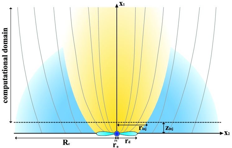
Figure 1: Schematic illustration of the simulation setup. The $x_{3}$ direction is perpendicular to the displayed image, and shows similar features as in the $x_{2}$ direction. The zero-point on the $x_{1}$ axis is on the protostar. Also shown is the disk, the injection region, outflow, and core infall envelope. The gray lines illustrate the shape of the initial magnetic field lines.

Table 1: Summary of the setup parameters for the simulations. $m_{*}$ is the mass of the protostar, $\dot{m}_{*}$ is the accretion rate onto the protostar, $r_{*}$ is the radius of the protostar, $r_{d}$ is the radius of the disk, $r_{\rm inj}$ is the radius of the injection region, $v_{\rm K*}$ is the Keplerian speed at the protostellar surface, $\rho_{\rm 0}$ is the injection density on the axis, $\rho_{\rm env,out}$ is the density at the core boundary, $B_{*}$ is the disk magnetic field at the surface of the protostar, $\dot{m}_{\rm inj}$ is the rate of outflow mass injection (into one hemisphere; equal to 5% of $\dot{m}_{*}$), and $\dot{p}_{\rm inj}$ is the rate of momentum injection (into one hemisphere).

$m_{*}$	$\dot{m}_{*}$	$r_{*}$	$r_{d}$	$r_{\rm inj}$	$v_{\rm K*}$	$\rho_{0}$	$\rho_{\rm env,out}$	$B_{\rm*}$	$\dot{m}_{\rm inj}$	$\dot{p}_{\rm inj}$
$[M_{\odot}]$	$[M_{\odot}~{}{\rm\>yr^{-1}}]$	$[R_{\odot}]$	$[{\rm au}]$	$[{\rm au}]$	$[{\rm km~{}s^{-1}}]$	$[{\rm cm^{-3}}]$	$[{\rm cm^{-3}}]$	$[{\rm G}]$	$[M_{\odot}~{}{\rm\>yr^{-1}}]$	$[M_{\odot}~{}{\rm\>yr^{-1}}~{}{\rm km~{}s}^{-1}]$
$1$	$1.01\times 10^{-4}$	2.61	13.1	91.9	270.31	$2.9\times 10^{8}$	$1.6\times 10^{6}$	324.35	$5.05\times 10^{-6}$	$0.0025$
$2$	$1.42\times 10^{-4}$	3.45	20.9	105.7	332.50	$1.7\times 10^{8}$	$1.6\times 10^{6}$	305.58	$7.10\times 10^{-6}$	$0.0050$
$4$	$1.95\times 10^{-4}$	20.5	34.2	123.7	192.90	$2.3\times 10^{7}$	$1.5\times 10^{6}$	68.152	$9.75\times 10^{-6}$	$0.0047$
$8$	$2.67\times 10^{-4}$	33.4	57.1	150.0	213.73	$1.1\times 10^{7}$	$1.3\times 10^{6}$	51.105	$1.34\times 10^{-5}$	$0.0071$
$16$	$3.19\times 10^{-4}$	6.41	101.0	196.4	689.95	$3.3\times 10^{7}$	$1.0\times 10^{6}$	271.99	$1.60\times 10^{-5}$	$0.021$
$24$	$3.34\times 10^{-4}$	6.38	185.0	282.0	848.6	$2.0\times 10^{7}$	$7.4\times 10^{5}$	262.83	$1.67\times 10^{-5}$	$0.025$

2.5 Calculating the outflow opening angle $\theta_{\rm outflow}$

We are particularly interested in the opening angle ($\theta_{\rm outflow}$) of the outflow, since this is a quantity that is directly related to the star formation efficiency and is a measurable quantity in real protostellar cores. It was also calculated by Zhang et al. (2014b), and can therefore be compared with their work. To calculate it, we search through the grid (at $x_{1}=R_{\rm c}$) for forward velocities $v_{1}>c_{s}=0.6~{}{\rm km~{}s^{-1}}$. Starting from the outside grid boundary, we seek through the grid along the principal axes towards the central rotation axis, and take the first instance of such velocity to be the edge of the flow. We then draw a straight line from there to the protostar (the center of the core). The angle that this line makes with the normal to the disk we define to be $\theta_{\rm outflow}$. As the flow is not entirely symmetric, we do this along both the $x_{2}$ and the $x_{3}$ directions, from both boundaries, and take $\theta_{\rm outflow}$ to be the average of these. If the opening angle is so large that the outflow escapes through the side boundaries, then the angle is calculated at the height at which it escapes, using a similar procedure as described above.

2.6 Cases with a pre-cleared cavity

As described above, our first set of simulations ignore the earlier evolutionary stages in the development of the outflow cavity. To explore the potential effects of this approximation, we run another sequence of models with $m_{*}=4,\>8,\>16$, and $24\>{M_{\odot}}$, with each model having a cavity pre-cleared based on the results of the lower mass model without pre-clearing. In the pre-cleared region, we simply reduced the density by a factor of ten compared to the simulation without pre-clearing. The boundary of the pre-cleared region was defined to be:

$$r_{\rm cyl}=r\sin\theta_{\rm clearing}+50\left(\frac{R_{\odot}}{r_{*}}\right){\rm au}$$ (6)

where $\theta_{\rm clearing}$ is the opening angle $\theta_{\rm outflow}$ of the previous lower-mass simulation (Table 2), and $r_{\rm cyl}$ and r are, as before, the cylindrical distance from the axis and the distance from the protostar. This expression was found to mimic the cavity found in the simulations without pre-clearing reasonably well.

3 Results

3.1 General outflow morphologies and velocity distributions

We perform a sequence of disk wind protostellar outflow simulations with the protostellar mass increasing from 1 to 24 $M_{\odot}$ and the initial envelope mass declining from $59~{}{M_{\odot}}$ to $28~{}{M_{\odot}}$, which maintains the constant total of $60\>M_{\odot}$ (of the envelope, the protostar, and the disk; see above). We show the density slices at $x_{3}=0$ in Figure 2 at the end of the simulations. Figure 3 shows the same, but only showing the material with a velocity component $v_{1}>c_{s}$. Overlayed on that are yellow lines showing the opening angle as found in Zhang et al. (2014b), and blue lines showing the opening angle that we find in this work. As we discuss in more detail below, we find a good agreement between the opening angle in this work and the analytic calculations of Zhang et al. (2014b). In all simulations, the outflow carves out a low density cavity. However, some higher density gas outside of this cavity is also outflowing, and $\theta_{\rm outflow}$ is therefore larger than just the size of the cavity. As described in §2, the time of the snapshots shown in Figure 2 is after an amount of time needed for the star to accrete half of the mass needed to bring it to the next simulated model.

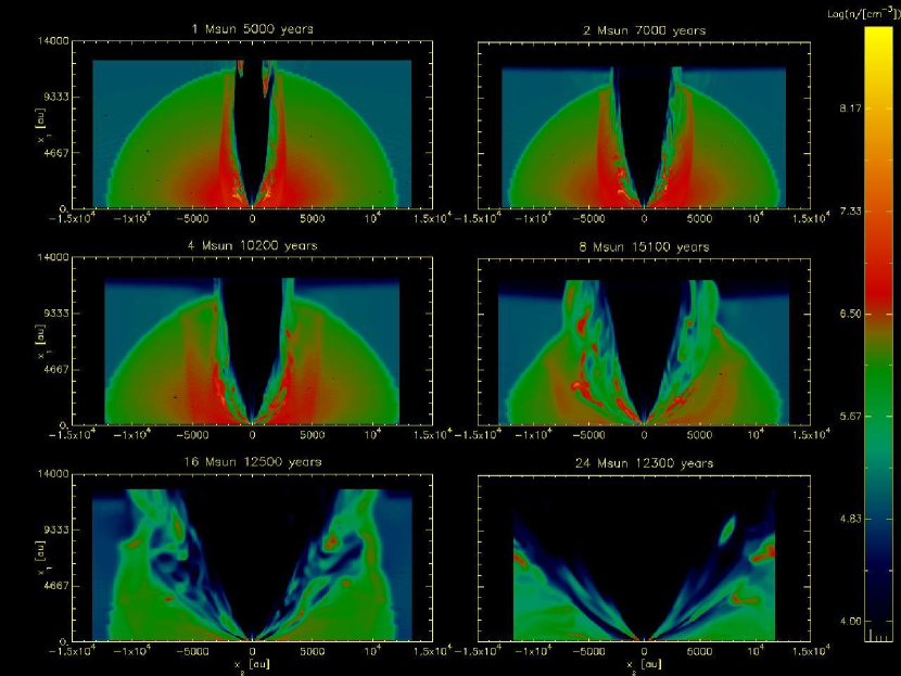
Figure 2: Slices through the middle of the simulation domains (in the $x_{1}$ - $x_{2}$ plane) showing density structures ($n_{\rm H}$) of the massive protostellar cores for fiducial runs with protostellar masses of 1, 2, 4, 8, 16, and 24 ${M_{\odot}}$, as labelled. Outputs are shown after various amounts of time evolution (see text).

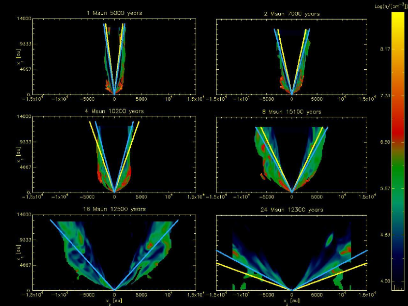
Figure 3: The same as Fig. 2, but only showing the density that has a positive velocity in the $x_{1}$ direction greater than the sound speed ($v_{1}>c_{s}$). This therefore shows the structure of the outflow. The yellow “V”-shaped lines show $\theta_{\rm outflow}$ found in the semi-analytic models of Zhang et al. (2014b), while the light blue “V”-shaped lines show the opening angle that we find in this work. Note that in the $16~{}{M_{\odot}}$ simulation, the blue and yellow lines are on top of each other, as the opening angle that we found matches that from Zhang et al. (2014b).

In Figure 4 we show histograms of the distribution of the outflowing mass from one hemisphere with respect to the outflow velocity ($v_{1}$), first at an early stage of the simulations near the point of first break out from the core, and then at the end of the simulations. In the former, the lower mass simulations show a local peak around $10~{}{\rm km~{}s^{-1}}$, while in the higher mass cases this peak rises to around $30~{}{\rm km~{}s^{-1}}$. We will compare these distributions with observed systems below.

In Figure 5 we show the distribution of the outflowing mass with respect to the outflow density, at the end of each simulation. Most outflowing mass in the $24~{}{M_{\odot}}$ simulation is found to be around $n_{\rm H}\sim 10^{5}-10^{6}~{}{\rm cm^{-3}}$. For the lower-mass simulations, the distribution is bimodal with most mass at a density of around $2\times 10^{6}~{}{\rm cm^{-3}}$ and another, smaller peak at $\sim 10^{5}~{}{\rm cm^{-3}}$. The $16~{}{M_{\odot}}$ simulation is in between, with a much broader peak stretching from $\sim 5\times 10^{4}$ to $\sim 10^{6}~{}{\rm cm^{-3}}$.

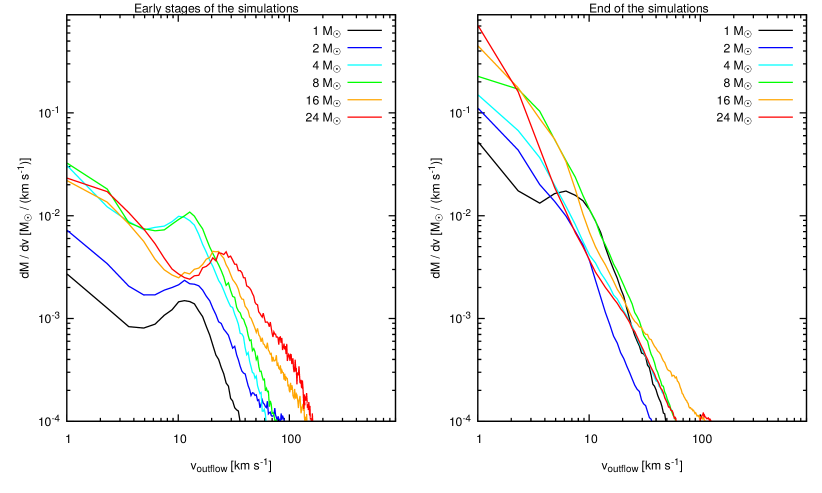
Figure 4: Left panel: Histogram showing the distribution of the outflow mass with respect to the outflow speed, evaluated around the time that the outflow breaks out of the core in each simulation. The bin width is $1.3~{}{\rm km~{}s^{-1}}$. Right panel: the same, but at the end of the simulations, at which point much of the original mass has left the computational domain.

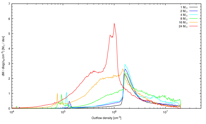
Figure 5: Distribution of the outflow mass with respect to the logarithm of H number density. The histogram is made from the last snapshot of each simulation. The bin width is 0.01 dex.

In Figure 6 we show a slice of the magnetic field strength at the end of each simulation. It is evident that the magnetic field strength within the outer part of the outflow cavity is relatively weak, with $B\ll 1~{}{\rm mG}$, i.e., much lower than the background core’s ambient magnetic-field. The magnetic-field strengths at the base of the outflow are much stronger, with values approaching $\sim 100$ mG in the highest mass cases.

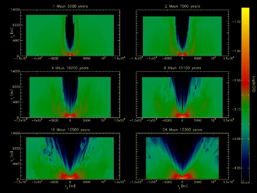
Figure 6: Slices through the middle of the grid showing the logarithm of the magnetic field strength at the end of each simulation.

In these simulations the plasma $\beta$ ($\beta=P_{\rm gas}/P_{B}$ is the ratio of the gas pressure $P_{\rm gas}$ to the magnetic pressure $P_{B}$) is for the most part much less than unity (i.e., the magnetic pressure dominates). Dynamical (ram) pressures due to gas flows can be even more important. Thus, instead of the plasma-$\beta$, we show in Figure 7 the ratio of the sum of the gas pressure and the dynamical pressure to the magnetic pressure, i.e., $\beta^{\prime}=(P_{\rm gas}+P_{\rm dyn})/P_{B}$, where $P_{\rm dyn}=\rho(v_{1}^{2}+v_{2}^{2}+v_{3}^{2})/2$. Figure 7 also shows a yellow curve outlining where the dynamical pressure equals the magnetic pressure, and a white curve outlining where the gas pressure equals the magnetic pressure. In the outflow cavity $\beta^{\prime}>1$ and the dynamical pressure is by far the most dominant. The exception is for the lowest protostellar masses, where the gas pressure is also found to contribute significantly in and around the outflow cavity. Outside of this region, the magnetic pressure is the dominant pressure term almost everywhere.

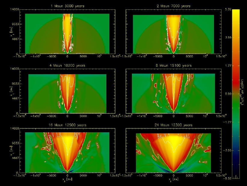
Figure 7: Slices through the middle of the grid showing the logarithm of the sum of the gas pressure and the dynamical pressure, divided by the magnetic pressure ($\beta^{\prime}$), at the end of each simulation. The yellow line outlines where the dynamical pressure equals the magnetic pressure. The white line outlines where the gas pressure equals the magnetic pressure.

3.2 Outflow opening angle

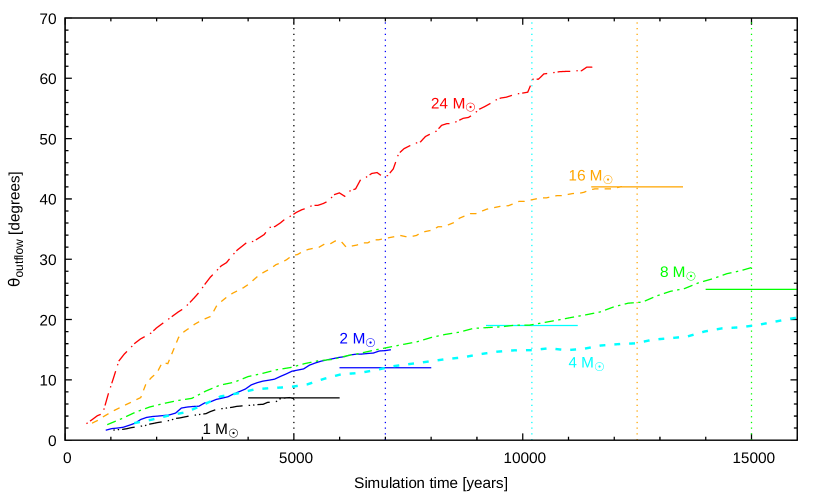
Figure 8: Opening angle of outflow cavity, $\theta_{\rm outflow}$, as a function of simulation time for the runs with protostellar masses of $1~{}{M_{\odot}}$ (black dot-dot-dash), $2~{}{M_{\odot}}$ (solid blue line), $4~{}{M_{\odot}}$ simulation (cyan dashed line), $8~{}{M_{\odot}}$ (green long-dash short-dash line), $16~{}{M_{\odot}}$ (orange dashed line) and $24~{}{M_{\odot}}$ (red long-dash dot line) for the case with no pre-cleared cavity. The colored vertical dotted lines show the times when the stars have accreted half the mass needed to take it to the next simulated model in the sequence. The horizontal line portions crossing the vertical lines indicate the opening angles found in the semi-analytic models of Zhang et al. (2014b).

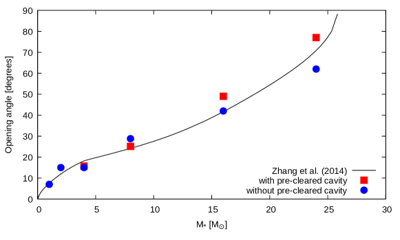
Figure 9: Outflow opening angle versus protostellar mass. Blue circles are the opening angles found in our fiducial simulations without pre-clearing. Red squares are the opening angles in the simulations with pre-clearing. The black line shows the results of the semi-analytic model of Zhang et al. (2014b).

Table 2: The final opening angle ($\theta_{\rm outflow}$) found in the simulations for the various protostellar masses, after a time when the star would have accreted half the mass needed to take it to the next simulated protostellar mass (the $24~{}{M_{\odot}}$ simulation has accreted $4~{}{M_{\odot}}$). Also listed is the total mass that has flowed out of one hemisphere during each simulation.

Mass of star	$\theta_{\rm outflow}$	$\theta_{\rm outflow}$	Total mass outflow	Total mass outflow
	w/o pre-clearing	w/ pre-clearing	w/o pre-clearing	w/ pre-clearing
$[{M_{\odot}}]$	[degrees]	[degrees]	$[{M_{\odot}}]$	$[{M_{\odot}}]$
1	8.4	-	0.35	-
2	15.0	-	0.88	-
4	14.9	15.7	0.70	0.28
8	28.8	25.1	1.60	1.06
16	42.0	49.0	2.75	2.05
24	62.0	77.0	3.34	2.38

Figure 8 shows the time evolution of $\theta_{\rm outflow}$ in each of the fiducial simulations, i.e., without pre-clearing. In each individual simulation $\theta_{\rm outflow}$ grows from zero from the time when the outflow has just managed to break out of the initial core envelope structure, typically after $\lesssim 1,000\>$years, depending on $m_{*}$. In the case of the $m_{*}=$1, 2, 4 and 8 $M_{\odot}$ runs, $\theta_{\rm outflow}$ then increases fairly steadily. For the 16 $M_{\odot}$ case, there is more rapid initial expansion as the outflow cavity is established, and then a more distinct phase of gradual widening. Finally for the 24 $M_{\odot}$ case, the expansion is fast and quite steady for the full duration of the simulated period, with only a modest decrease in the rate of expansion during the later evolution.

As described above, a natural time to consider the outputs of the simulation is after the protostar has had sufficient time to increase its mass significantly, i.e., half-way towards the next model in the sequence. These times are used to evaluate the “final” $\theta_{\rm outflow}$ that is listed in Table 2. In Figure 8, these times are marked by vertical dotted lines. Also shown in this figure are the values of $\theta_{\rm outflow}$ expected in the semi-analytic model of Zhang et al. (2014b). At our adopted output times, these semi-analytic estimates compare very well with those of our MHD simulations: they are generally within about 5 degrees of each other.

At a given time, including our chosen “final” output times, $\theta_{\rm outflow}$ is generally larger for models with more massive protostars. This can also be seen in Figure 9, which shows $\theta_{\rm outflow}$ versus protostellar mass. The main exception is the $4\>M_{\odot}$ case, which has a slightly smaller $\theta_{\rm outflow}$ compared to the $2\>M_{\odot}$ case. The reason for this is that at $4\>M_{\odot}$ the protostar has evolved into a relatively large, expanded size, due to redistribution of entropy in the protostar, including effects of D shell burning (Palla & Stahler, 1991, 1992; Hosokawa & Omukai, 2009; Hosokawa et al., 2010). This means the Keplerian speed at the disk inner edge is relatively low so that the disk wind outflow is relatively weak. For this case, the effects of pre-clearing, discussed below, are expected to be more important. Figure 9 also compares our simulation results to the semi-analytic model estimates of Zhang et al. (2014b). It is apparent that the numerical results agree well with the semi-analytic model predictions.

In addition to the simulations described above, we performed a sequence of simulations where the initial setup has a pre-cleared cavity (starting with the $4~{}{M_{\odot}}$ simulation) (see §2.6). We find that $\theta_{\rm outflow}$ (see Table 2 and Figure 9) is not much different whether or not we have pre-cleared a cavity, which indicates the general robustness of the results and the validity of ignoring prior evolution for each fiducial simulation run.

However, $\theta_{\rm outflow}$ in the $24~{}{M_{\odot}}$ simulation with pre-clearing does open up faster and to a moderately greater extent ($\theta_{\rm outflow}=77.0^{\circ}$) than in the simulation without pre-clearing ($\theta_{\rm outflow}=62.0^{\circ}$). Interestingly, in the $8~{}{M_{\odot}}$ simulation, $\theta_{\rm outflow}$ is smaller with pre-clearing than without. This may be due to the outflow feedback being more easily directed into the low-density initial cavity, i.e., deflecting off the dense core infall envelope, and so more easily confined. In the case without the initial cavity, the outflow may be able to establish a broader opening angle during its initial break-out phase.

3.3 Mass flow rate and momentum rate

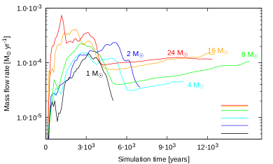
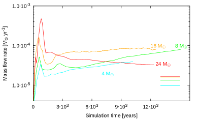
Figure 10: The mass flow rate (in one hemisphere) as a function of time for the simulations without pre-clearing (left panel), and with pre-clearing (right panel). The horizontal lines in the right side of the figures show the injected mass flow rate, for comparison.

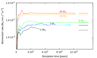
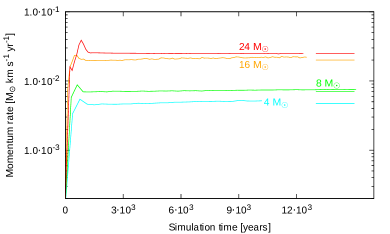
Figure 11: The momentum flow rate (in one hemisphere) as a function of time for the simulations without pre-clearing (left panel), and with pre-clearing (right panel). The horizontal lines in the right side of the figures show the injected momentum rate, for comparison.

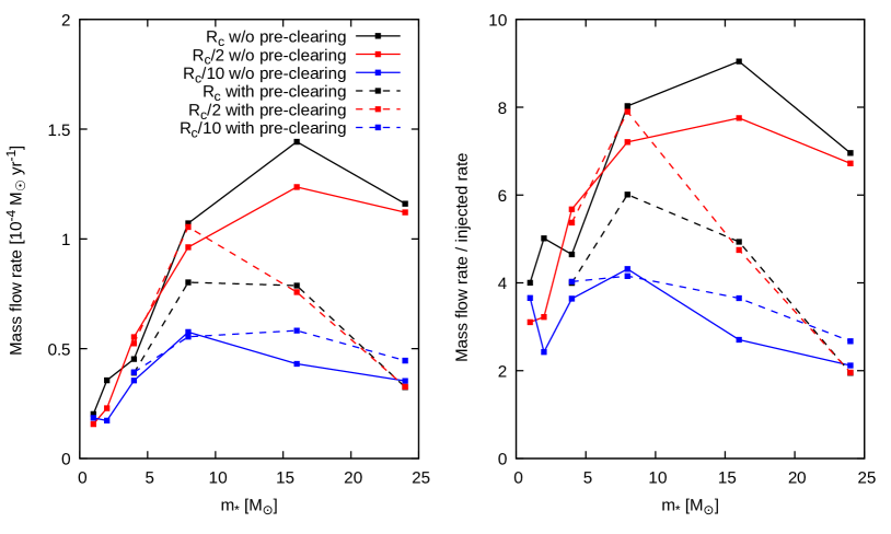
Figure 12: Mass outflow rate at end of the simulations (in one hemisphere) at a height above the disk of $1/10~{}R_{\rm c}$ (blue curve), $1/2~{}R_{\rm c}$ (red curve), and $R_{\rm c}$ (black curve) as a function of the protostellar mass (left panel). The right panel show the same, but normalized to the injected flow rate (into one hemisphere). The solid lines are the simulations without a pre-cleared cavity, while the dashed lines are the simulations with a pre-cleared cavity.

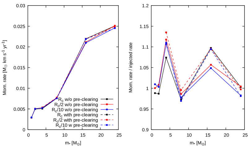
Figure 13: The outflowing momentum rate at the end of the simulations (in one hemisphere) at a height above the disk of $1/10~{}R_{\rm c}$ (blue curve), $1/2~{}R_{\rm c}$ (red curve), and $R_{\rm c}$ (black curve) as a function of the protostellar mass (left panel). The right panel show the same, but normalized to the injected rate (into one hemisphere). The solid lines are the simulations without a pre-cleared cavity, while the dashed lines are the simulations with a pre-cleared cavity.

Figures 10 and 11 show the mass outflow and momentum flow rates measured at a height of $R_{c}$ above the disk, as a function of time for our simulations. Here the mass outflow rate ($\dot{m}=\int\rho vdx_{2}dx_{3}$, for $v_{1}>c_{s}$) is the mass flowing out of one hemisphere in the $x_{1}$ direction only, and likewise the momentum flow rate ($\dot{p}=\int\rho v^{2}dx_{2}dx_{3}$, for $v_{1}>c_{s}$) is only including the momentum in the $x_{1}$ direction, again from one hemisphere. Without pre-clearing, the flow rate for each simulation has a large “bump” in the early part of the simulation. This bump is a result of the initial state. In each simulation, the flow has to clear out a new outflow channel, leading to this artificial transient event. Once an outflow channel has been established by pushing the mass out of the simulation box, the flow rate stabilizes. The effect of the pre-clearing is apparent in the mass outflow rate figure. With pre-clearing, there is still a “bump”, but it is much less prominent. We see from Figure 10 that the mass flow rate out of the core at the end of the simulations is always larger than the injected mass flow rate by a factor of a few. The larger flow rate out of the core is due to erosion of the infalling envelope. In the $24~{}{\rm M_{\odot}}$ simulation with pre-clearing, the mass flow rate gradually drops. This is due to there not being much mass to sweep up.

The momentum flow rates also stabilize after an initial transient phase ($\sim 5-10\times 10^{-3}~{}M_{\odot}~{}{\rm km~{}s^{-1}\>yr^{-1}}$ for the 4 and 8 ${M_{\odot}}$ simulations and $\sim 2\times 10^{-2}~{}M_{\odot}~{}{\rm km~{}s^{-1}\>yr^{-1}}$ for the 16 and 24 ${M_{\odot}}$ simulations). The effect of the pre-clearing is also visible in the momentum rates, in that these are smoother at earlier times with pre-clearing than without. The mass flow and momentum rates stabilizes around the same values in the simulations with and without pre-clearing. This value is roughly equal to the injected momentum rate.

In Figure 12 we show the mass outflow rate at the end of each simulation at different heights above the disk in the envelope (at $R_{c}$, $R_{c}/2$, and $R_{c}/10$) as a function of the protostellar mass for both the simulations without and with pre-clearing. We find that the mass outflow rate at $x_{1}=R_{c}$ generally is larger for larger protostellar mass. This is mainly due to the stronger injection (see Table 1). As the outflowing material makes its way through the envelope, mass is being swept up. As a consequence, the mass flow rate at $R_{\rm c}$ is a factor 4-10 times the injected mass flow rate, it is generally larger than deeper in the core, and it is larger in the simulations without pre-clearing.

Figure 13 shows the outflow momentum rate at the end of each simulation at different heights above the disk in the core as a function of protostellar mass. We find that the momentum flow rate increases as $m_{*}$ rises, reaching a few $\times 10^{-2}~{}M_{\odot}~{}{\rm km~{}s^{-1}\>yr^{-1}}$, and that it remains approximately constant as the flow propagates through the core, starting from the injection boundary.

The total mass flowing out of one hemisphere (found by integrating the mass outflow rate over time) for each case is listed in Table 2. Summing all the simulations without pre-clearing, we find that $9.62~{}{M_{\odot}}$ flowed out of one hemisphere in our simulations. With pre-clearing, the sum is $5.77~{}{M_{\odot}}$, though that excludes the $1$ and $2~{}{M_{\odot}}$ simulations. Since the simulations only run to half-way to accreting to the next stage, then the total mass ejected if continuous growth of the protostar were followed is expected to be about twice the above values, i.e., $2\times\sim 6\>M_{\odot}\simeq 12\>M_{\odot}$ in the case with pre-clearing. Accounting for both hemispheres, the total outflowing mass becomes $\sim 24~{}{M_{\odot}}$, which is similar to the mass growth of the protostar, demonstrating that the star formation efficiency is about 50% from the core during this evolution.

3.4 Effects of injected flow rotation and an unmagnetized outflow

We find that in the $16~{}{M_{\odot}}$ simulation (without pre-clearing), after $10^{4}$ years, there is very little difference whether the injected material is given rotation or not (see Figure 14). In both cases the opening angle at this particular time is $42^{\circ}$.

In a test simulation of the same $16~{}{M_{\odot}}$ case without magnetic field we find that the opening angle is $48^{\circ}$. This illustrates the role of the magnetic pressure in confining the flow. Without a magnetic field, the flow will open up until $P_{\rm dyn}$ is approximately balanced by $P_{\rm gas}$. Accordingly, we also find that the no magnetic field simulation has a larger outflowing mass rate than the simulation with magnetic field, due to the larger opening angle of the outflow. The simulation with magnetic field has a mass flow rate out of one hemisphere of $2.2\times 10^{-4}~{}{M_{\odot}{\rm\>yr^{-1}}}$, while that without magnetic field has a mass flow rate of $3.1\times 10^{-4}~{}{M_{\odot}{\rm\>yr^{-1}}}$, i.e., 1.4 times greater.

One noticeable difference, however, is that without a magnetic field, the outflow is not capable of maintaining a clear outflow cavity. Another difference is that the density of the remaining envelope material outside of the outflow cavity is an order of magnitude larger in the simulation without magnetic field, as seen in Figure 14. Without the magnetic field to confine and collimate the outflow, the wider angle flow interacts with more of the collapsing envelope, pushing and compressing it and thus causing the higher densities seen in the figure.

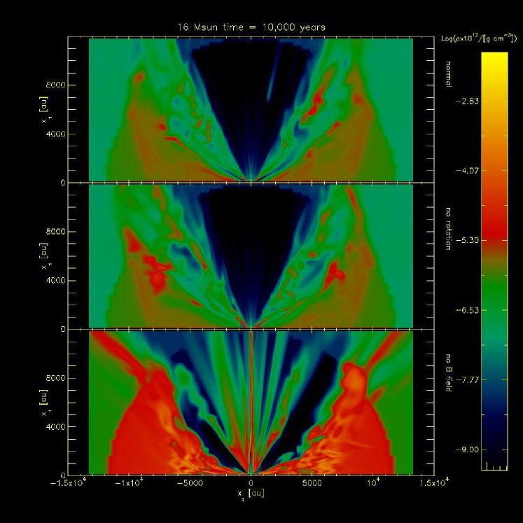
Figure 14: The $16~{}{M_{\odot}}$ simulation after $10^{4}$ years. The top panel shows the normal simulation, the middle panel shows the same setup except that the injected material is not given a rotational velocity. The bottom panel shows the same setup as the top panel, but with no magnetic field.

3.5 Dependence on numerical resolution

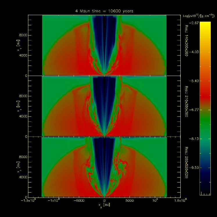
Figure 15: Comparison of the density structure through the middle of the grid of the $4~{}{M_{\odot}}$ simulation in normal resolution (top panel), medium resolution (middle panel), and high resolution (bottom panel) after 10,200 years of simulation time.

As described in §2, we used a grid with $140\times 260\times 260$ cells in our standard setup for these simulations (with $m_{*}\geq 4~{}{M_{\odot}}$). To test the effect of grid resolution on the results, we also ran the $4~{}{M_{\odot}}$ simulation using a grid with $210\times 380\times 380$ cells (medium resolution), and using a grid with $280\times 520\times 520$ cells (high resolution). Figure 15 compares the results of these simulations after 10,200 years of simulation time, at which point the protostar would have accreted $2~{}{M_{\odot}}$. While some differences are apparent in the density structures, the opening angle of the flow is found to be approximately the same in all three cases. In particular, $\theta_{\rm outflow}$ in the standard, medium and high resolution simulations was found to be $14.9^{\circ}$, $16.5^{\circ}$ and $18.2^{\circ}$, respectively.

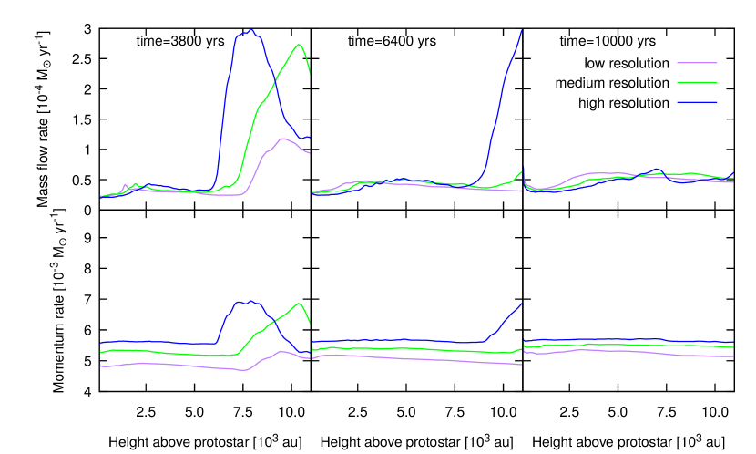
Figure 16: The mass flow rate (top row), and momentum rate (bottom row) throughout the core at three different times in the $4~{}{\rm M_{\odot}}$ simulation, for the low resolution simulation (purple), medium resolution simulation (green), and high resolution simulation (blue).

In all of these resolution test runs, the flow begins to break out of the core after approximately 1,000 years. We find that the mass flow rate, differs a lot between the different resolutions at earlier times (see Figure 16). After 6,400 years we find the largest difference, with the mass flow rate out of the core in the high resolution simulation being almost an order of magnitude larger than in the low-resolution simulation. However, after 10,000 years the mass flow rates in the different resolution simulations appear to be converging towards $\approx 5\times 10^{-5}~{}{M_{\odot}{\rm\>yr^{-1}}}$. The difference is related to the clearing of the outflow cavity, with the higher resolution run taking longer time to push the material out of the simulation box.

The momentum rate does not show the same level of differences, and after 6,400 years the momentum rate in the high resolution simulation is only a factor 1.5 larger than in the low-resolution simulation, which is the largest deviation between the simulations that we find. After 10,000 years the momentum rate in the high resolution simulation is $\approx 10\%$ larger than in the low resolution simulation. Again the differences are related to the clearing of the outflow cavity, see Figure 16. The slightly higher momentum rates in the high resolution simulation are due to the larger velocities being resolved in the central regions. We are therefore satisfied that the resolution does not significantly affect the results of our simulations. We caution that neither the mass flow rate nor the momentum rate is constant throughout the grid, so these values are subject to the exact slice and time at which they are calculated.

We recall that we use a logarithmic grid, and that we aim at resolving the injection radius $r_{\rm inj}$ with 10 cells (see §2). Since in the $1$ and $2~{}{M_{\odot}}$ simulations the injection region is the smallest, these simulations therefore have the smallest cells (in the $x_{2}$ and $x_{3}$ directions), which therefore necessitates the biggest stretching of the grid in order to extend the grid beyond $R_{\rm c}$, when using the same number of cells. The cells around the axis near the inner $x_{1}$ boundary are cubic by design, so this also lead to small cells in the $x_{1}$ direction near the injection boundary. In these $1$ and $2~{}{M_{\odot}}$ simulations, we found that when using the same resolution as the higher protostellar masses, the envelope develops a “noisy” density structure over time. This turned out to be related to the degree of stretching of the grid that we had to utilize to both resolve the injection radius with $\sim 10$ cells, and resolve the whole envelope structure. Using more grid cells (in all directions, but in particular in the $x_{1}$ direction), we found that we could reduce the noisiness of these simulations, however, the main results, i.e., $\theta_{\rm outflow}$ and $\dot{m}$, were not affected.

4 Discussion and Summary

In our presented MHD simulations, we follow a sequence of evolutionary models of the protostar, enabled by injecting a disk wind into the simulation box at a height of $100~{}{\rm au}$ above the disk. A number of other groups have performed collapse simulations to study outflows from massive protostars, using various numerical techniques and including different physics. However, most of these do not follow the evolution of the protostar until the end, and therefore can not estimate the full evolution of the morphology, outflow properties and the star formation efficiency.

4.1 Comparison to previous theoretical work

Some previous studies performed ideal-MHD simulations of $100~{}{M_{\odot}}$ core collapse (Seifried et al., 2011, 2012; Hennebelle et al., 2011; Commerçon et al., 2011). Those MHD simulations showed especially that fragmentation is suppressed by magnetic pressure and magnetic breaking in the highly magnetized cases. However, they could not continue the simulation long enough to reach a $\sim 5~{}{M_{\odot}}$ protostellar mass due to the high numerical cost of following the small-scale processes, i.e., disk formation and outflow launching.

The collapse of a massive cloud core was also simulated by Matsushita et al. (2017, 2018). Starting from a range of cloud masses, they followed the protostar until it reached a mass of $\lesssim 30~{}{\rm M_{\odot}}$. For their simulations with cloud masses of $32$ and $77~{}{\rm M_{\odot}}$ (their simulations most comparable to our setup), they stopped the simulations when the protostar was a few solar masses. At their highest resolution, they have a resolution of $0.8~{}{\rm au}$, a factor of 6 smaller than in our highest resolution simulations. In their simulation with a cloud mass of $77~{}{M_{\odot}}$, they found a similar mass ejection rate ($\sim 10^{-4}~{}{M_{\odot}{\rm\>yr^{-1}}}$) to that which we found in our models.

However, since these works terminate the calculations before the star reaches its final mass, they do not estimate the star formation efficiency. This is one of the main objectives of our paper. We therefore simulated a sequence of models using boundary conditions relevant to the Turbulent Core Model that can be compared to the semi-analytic work of Zhang et al. (2014b).

We have found that the opening angle increases with more massive protostars, i.e., with age, in agreement with the evolutionary sequence proposed in Beuther & Shepherd (2005). Building on the model of Matzner & McKee (2000), Zhang et al. (2014b) evaluated the evolution of the outflow opening angle during the growth of a massive protostar. For their fiducial values, they found that a core with initial mass of $60~{}{M_{\odot}}$ reaches a stage with an $8~{}{M_{\odot}}$ protostar with an outflow with opening angle of $25^{\circ}$. Later it grows to a $16~{}{M_{\odot}}$ protostar having an outflow with an opening angle of $40^{\circ}$. The final star resulting from their model had a mass of $26~{}{M_{\odot}}$. This is in reasonably good agreement with what we find in our study. We note that this is also in agreement with observations (Arce et al., 2007).

Since we find similar results to those in Zhang et al. (2014b) for outflow opening angles, we therefore also obtain a SFE of $\sim 50\%$, similar to what they found. This is then an indication that such MHD disk winds may be a dominant mechanism for limiting the growth of the protostar and ultimately helping to shape the stellar initial mass function from a given pre-stellar core mass function.

Radiative feedback is also expected to have a significant impact on the formation of massive stars (Krumholz et al., 2009; Kuiper et al., 2010; Klassen et al., 2016; Rosen et al., 2016). However, the magnetically-driven outflow creates the cavity before the luminosity becomes sufficiently high to interfere with the mass accretion. Since the outflow cavity channels the radiation, the impact of radiative feedback is reduced (Yorke & Bodenheimer, 1999; Krumholz et al., 2005; Kuiper et al., 2015). Recent studies including multiple feedback processes together show, at least in the case of cloud cores with $M_{c}<100~{}{M_{\odot}}$, that the MHD disk wind is likely to be the dominant feedback mechanism determining the SFE (Tanaka et al., 2017; Kuiper & Hosokawa, 2018). Based on these results, we conclude that the radiative processes would not alter our results significantly.

We note that a limitation of applying our work to link CMF and IMF is that we have focused on single stars, but most massive stars are in binaries (Sana et al., 2012). Kuruwita et al. (2017) simulated outflows from the formation of both single and binary stars. While their simulations could not predict the final masses of the stars due to computational limitations, they found that the single star case accreted less mass compared to the binaries in the same amount of time. Hence single stars may have a lower star formation efficiency than binary stars. Such an effect may be due to the relatively weaker outflows from two lower mass protostars compared to that of a single protostar with twice the mass.

4.2 Comparison to observations

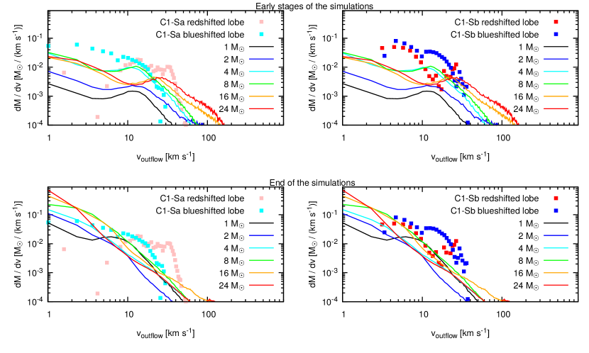
Figure 17: The same as Figure 4; histograms showing the distribution of the outflow mass with respect to the outflow speed, evaluated around the time that the outflow breaks out of the core in each simulation (top row), and at the end of each simulation (bottom row). In the left panels, observed data of protostar C1-Sa is shown, and in the right panels, observed data of protostar C1-Sb is shown (Tan et al., 2016).

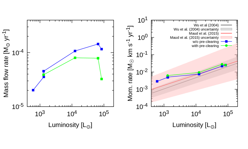
Figure 18: The mass flow rate (left panel) and momentum rate (right panel) in one hemisphere as a function of bolometric luminosity. The blue curve is for the simulations without pre-clearing, the green curve is for the simulations with pre-clearing. The solid gray line is the best fit from Wu et al. (2004), the gray shaded area indicates the uncertainty, while the solid red line is the best fit from Maud et al. (2015) and the pink shaded area indicates the uncertainty. Note that there are two blue points roughly on top of each other in the momentum rate plot at a luminosity of $\sim 1.3\times 10^{3}~{}{\rm L_{\odot}}$

.

We have compared the distributions of outflowing masses in our simulations with some observed cases (Figure 17), i.e., those found in the protostars C1-Sa and C1-Sb (Tan et al., 2016). In the blueshifted outflow, they found the majority of the outflowing material at velocities well below $10~{}{\rm km~{}s^{-1}}$, while in the redshifted outflow it is more evenly distributed to $\sim 30~{}{\rm km~{}s^{-1}}$, especially in C1-Sa. The observed distributions appear to drop off with a steeper power law at high velocities than in our simulations. We find that generally the power law is steeper in the lower protostellar mass simulations than in the higher mass cases.

C1-Sa’s redshifted outflow and C1-Sb’s blueshifted outflow show significantly larger amounts of mass at higher velocities (and note that these distributions are not corrected for inclination, so once corrected would actually be even higher). We note, however, that the outflow properties from these sources were measured on scales extending $12^{\prime\prime}$ from the protostar, or 60,000 au. This is much larger than our simulation box of $\sim 12,000~{}{\rm au}$. In our simulations, much material, and in particular high velocity material, has left the simulation box (see Table 2). We therefore find it interesting that we roughly recover the bumps seen in the observed redshifted curves around $10$ and $30~{}{\rm km\>s^{-1}}$ at early times, before (especially high velocity) mass has been lost from the simulation box. These bumps, however, are related to the initial clearing of the outflow cavity for each simulation in the sequence, since these bumps are much less prominent in the simulations with pre-clearing. At later times, we recover the low velocity components reasonably well.

Maud et al. (2015) found outflow momentum rates of $10^{-3}-10^{-1}~{}M_{\odot}~{}{\rm km~{}s^{-1}{\rm\>yr^{-1}}}$ for outflows from core masses of $\sim 60~{}{M_{\odot}}$ (luminosity of $\sim 10^{3}-10^{5}~{}{L_{\odot}}$), while Beuther et al. (2002) also found momentum rates of $\sim 10^{-3}-10^{-1}~{}{M_{\odot}~{}{\rm km~{}s^{-1}\>yr^{-1}}}$ for such outflows. This is in reasonable agreement with our results, which reflect our choice of input boundary conditions. We found momentum rates (leaving the core) of $5\times 10^{-3}-3\times 10^{-2}~{}M_{\odot}~{}{\rm km~{}s^{-1}{\rm\>yr^{-1}}}$. These works also found mass flow rates of the order $10^{-4}-10^{-3}~{}{M_{\odot}~{}{\rm\>yr^{-1}}}$ for sources with luminosity of $\sim 10^{3}-10^{5}~{}{L_{\odot}}$, which are also in reasonable agreement with our mass flow rates found to be $0.5-2.5\times 10^{-4}~{}M_{\odot}~{}{\rm\>yr^{-1}}$.

We show the stabilized (final) mass flow rates and momentum flow rates as a function of bolometric luminosity in Figure 18. The bolometric luminosity has been estimated based on the mass of the protostar following Zhang & Tan (2018). The figure also shows the best fit line for the momentum flow rate from the observational data in Wu et al. (2004), given by $\log(\dot{P}/({M_{\odot}~{}{\rm km~{}s^{-1}\>yr^{-1}}}))=(-4.92\pm 0.15)+(0.648\pm 0.043)\log(L_{\rm bol}/{L_{\odot}})$, and in Maud et al. (2015) given by $\log(\dot{P}/({M_{\odot}~{}{\rm km~{}s^{-1}\>yr^{-1}}}))=(-4.60\pm 0.46)+(0.61\pm 0.11)\log(L_{\rm bol}/{L_{\odot}})$.

We found that the momentum rate in our simulations (Figure 18) roughly follows the same trend as the best fit to the observational data in Wu et al. (2004). However, while our points from the higher-mass protostellar simulations are within the uncertainty range from Wu et al. (2004), the points from the lower-mass simulations are a factor a few above. Still, our simulations only follow the evolutionary track of one example massive protostar forming under one clump environmental mass surface density. Most lower luminosity sources in the observational samples are expected to be protostars forming from lower-mass prestellar cores, and may also be in systematically different environments. A proper comparison here will require simulating a broader range of prestellar core masses and environmental conditions and then sampling the core mass function to build a realistic population of protostars at different evolutionary stages.

In addition, we note that the data in Wu et al. (2004) has a large scatter of about two orders of magnitude on either side of the best fit line, and therefore even our points from the lower-mass protostellar simulations are in agreement with some of their data points. Also, the luminosity of a source depends on the viewing angle, as much of the luminosity from the accretion and the protostar will escape out through the outflow cavity, which can lead to large uncertainty in the measurement. There is also uncertainty related to the conversion of ${}^{12}\mathrm{CO}$ to outflow mass (Zhang et al., 2016), which can lead to the observed momentum rate being underestimated. Hence it is possible that even our low protostellar mass simulations are in better agreement with the best fit from Wu et al. (2004) than what it appears from Figure 18. Compared with Wu et al. (2004), Maud et al. (2015) found a very similar best fit line to their data, but have somewhat smaller scatter of the data.

Other observational constraints can be made by comparing magnetic-field strengths in our simulations with observed values. The magnetic field in massive cores from which massive stars form was measured by Beuther et al. (2018). They found field strengths of $\sim 0.6-3.7~{}{\rm mG}$ in the high-mass starless region IRDC 18310-4. Our initial setup, with a core scale mG magnetic field, is in reasonable agreement with these findings. Then for later stages, Vlemmings et al. (2010) found that in high density material in Cep A where the masers occur, the magnetic field strength is $\sim 23~{}{\rm mG}$. Observations have found a field strength of $\sim 10~{}{\rm mG}$ in high density regions near the disk in the high-mass protostar IRAS 18089 (Vlemmings, 2008; Beuther et al., 2010; Dall’Olio et al., 2017). We find magnetic field strengths at the base of the outflow approaching 100 mG, in approximate agreement with the findings from Cep A, and the high density and near disk region of IRAS 18089. Surcis et al. (2009) and Dall’Olio et al. (2017) also found that the small scale field probed by the masers are consistent with large scale fields traced by dust.

4.3 Summary

In summary, we have performed 3 dimensional magneto-hydrodynamic simulations of outflows from protostars for a sequence of protostellar models forming from a $60~{}{M_{\odot}}$ prestellar core in a clump environment with mass surface density of 1 g cm^-2. We have found that the outflow generally becomes stronger and wider as the protostar grows in mass. The evolution of the outflow opening angle (Figure 9) agrees well with the semi-analytic model of Zhang et al. (2014b). The mass flow rates, momentum flow rates, and outflow masses in our simulations are in reasonable qualitative agreement with observations (Wu et al., 2004; Maud et al., 2015). With these simulations, and this particular mass configuration, we find a star formation efficiency of $\sim 50\%$, which is also in good agreement with the $\sim 43\%$ found by the analytic calculations performed by Zhang et al. (2014b).

References

- Anderson et al. (2006) Anderson, J. M., Li, Z.-Y., Krasnopolsky, R., & Blandford, R. D. 2006, ApJ, 653, L33
- André et al. (2010) André, P., Men’shchikov, A., Bontemps, S., et al. 2010, A&A, 518, L102
- Arce et al. (2007) Arce, H. G., Shepherd, D., Gueth, F., et al. 2007, Protostars and Planets V, 245
- Bacciotti et al. (2000) Bacciotti, F., Mundt, R., Ray, T. P., et al. 2000, ApJ, 537, L49
- Beltrán & de Wit (2016) Beltrán, M. T., & de Wit, W. J. 2016, A&A Rev., 24, 6
- Beuther et al. (2002) Beuther, H., Schilke, P., Sridharan, T. K., et al. 2002, A&A, 383, 892
- Beuther & Shepherd (2005) Beuther, H., & Shepherd, D. 2005, in Astrophysics and Space Science Library, Vol. 324, Astrophysics and Space Science Library, ed. M. S. N. Kumar, M. Tafalla, & P. Caselli, 105
- Beuther et al. (2010) Beuther, H., Vlemmings, W. H. T., Rao, R., & van der Tak, F. F. S. 2010, ApJ, 724, L113
- Beuther et al. (2018) Beuther, H., Soler, J. D., Vlemmings, W., et al. 2018, A&A, 614, A64
- Blandford & Payne (1982) Blandford, R. D., & Payne, D. G. 1982, MNRAS, 199, 883
- Bonnell et al. (2001) Bonnell, I. A., Bate, M. R., Clarke, C. J., & Pringle, J. E. 2001, MNRAS, 323, 785
- Bonnell et al. (1998) Bonnell, I. A., Bate, M. R., & Zinnecker, H. 1998, MNRAS, 298, 93
- Caratti o Garatti et al. (2015) Caratti o Garatti, A., Stecklum, B., Linz, H., Garcia Lopez, R., & Sanna, A. 2015, A&A, 573, A82
- Carrasco-González et al. (2010) Carrasco-González, C., Rodríguez, L. F., Anglada, G., et al. 2010, Science, 330, 1209
- Cheng et al. (2018) Cheng, Y., Tan, J. C., Liu, M., et al. 2018, ApJ, 853, 160
- Coffey et al. (2008) Coffey, D., Bacciotti, F., & Podio, L. 2008, ApJ, 689, 1112
- Commerçon et al. (2011) Commerçon, B., Hennebelle, P., & Henning, T. 2011, ApJ, 742, L9
- Dall’Olio et al. (2017) Dall’Olio, D., Vlemmings, W. H. T., Surcis, G., et al. 2017, A&A, 607, A111
- Hennebelle et al. (2011) Hennebelle, P., Commerçon, B., Joos, M., et al. 2011, A&A, 528, A72
- Hirota et al. (2017) Hirota, T., Machida, M. N., Matsushita, Y., et al. 2017, Nature Astronomy, 1, 0146
- Hosokawa & Omukai (2009) Hosokawa, T., & Omukai, K. 2009, ApJ, 703, 1810
- Hosokawa et al. (2010) Hosokawa, T., Yorke, H. W., & Omukai, K. 2010, ApJ, 721, 478
- Jørgensen et al. (2001) Jørgensen, M. A. S. G., Ouyed, R., & Christensen, M. 2001, A&A, 379, 1170
- Klassen et al. (2016) Klassen, M., Pudritz, R. E., Kuiper, R., Peters, T., & Banerjee, R. 2016, ApJ, 823, 28
- Kölligan & Kuiper (2018) Kölligan, A., & Kuiper, R. 2018, A&A, 620, A182
- Konigl & Pudritz (2000) Konigl, A., & Pudritz, R. E. 2000, Protostars and Planets IV, 759
- Könyves et al. (2010) Könyves, V., André, P., Men’shchikov, A., et al. 2010, A&A, 518, L106
- Krumholz et al. (2009) Krumholz, M. R., Klein, R. I., McKee, C. o. F., Offner, S. S. R., & Cunningham, A. J. 2009, Science, 323, 754
- Krumholz et al. (2005) Krumholz, M. R., McKee, C. F., & Klein, R. I. 2005, ApJ, 618, L33
- Kuiper & Hosokawa (2018) Kuiper, R., & Hosokawa, T. 2018, ArXiv e-prints, arXiv:1804.10211
- Kuiper et al. (2010) Kuiper, R., Klahr, H., Beuther, H., & Henning, T. 2010, ApJ, 722, 1556
- Kuiper et al. (2016) Kuiper, R., Turner, N. J., & Yorke, H. W. 2016, ApJ, 832, 40
- Kuiper et al. (2015) Kuiper, R., Yorke, H. W., & Turner, N. J. 2015, ApJ, 800, 86
- Kuruwita et al. (2017) Kuruwita, R. L., Federrath, C., & Ireland, M. 2017, MNRAS, 470, 1626
- Liu et al. (2018) Liu, M., Tan, J. C., Cheng, Y., & Kong, S. 2018, ApJ, 862, 105
- Lovelace et al. (1991) Lovelace, R. V. E., Berk, H. L., & Contopoulos, J. 1991, ApJ, 379, 696
- Lynden-Bell (1996) Lynden-Bell, D. 1996, MNRAS, 279, 389
- Machida & Matsumoto (2012) Machida, M. N., & Matsumoto, T. 2012, MNRAS, 421, 588
- Marti et al. (1993) Marti, J., Rodriguez, L. F., & Reipurth, B. 1993, ApJ, 416, 208
- Matsushita et al. (2017) Matsushita, Y., Machida, M. N., Sakurai, Y., & Hosokawa, T. 2017, MNRAS, 470, 1026
- Matsushita et al. (2018) Matsushita, Y., Sakurai, Y., Hosokawa, T., & Machida, M. N. 2018, MNRAS, 475, 391
- Matt & Pudritz (2005) Matt, S., & Pudritz, R. E. 2005, ApJ, 632, L135
- Matzner & McKee (2000) Matzner, C. D., & McKee, C. F. 2000, ApJ, 545, 364
- Maud et al. (2015) Maud, L. T., Moore, T. J. T., Lumsden, S. L., et al. 2015, MNRAS, 453, 645
- McKee & Tan (2002) McKee, C. F., & Tan, J. C. 2002, Nature, 416, 59
- McKee & Tan (2003) —. 2003, ApJ, 585, 850
- McLaughlin & Pudritz (1997) McLaughlin, D. E., & Pudritz, R. E. 1997, ApJ, 476, 750
- McLeod et al. (2018) McLeod, A. F., Reiter, M., Kuiper, R., Klaassen, P. D., & Evans, C. J. 2018, ArXiv e-prints, arXiv:1801.08147
- Moll (2009) Moll, R. 2009, A&A, 507, 1203
- Motte et al. (2018) Motte, F., Nony, T., Louvet, F., et al. 2018, Nature Astronomy, 2, 478
- Norman (2000) Norman, M. L. 2000, in Revista Mexicana de Astronomia y Astrofisica Conference Series, Vol. 9, Revista Mexicana de Astronomia y Astrofisica Conference Series, ed. S. J. Arthur, N. S. Brickhouse, & J. Franco, 66–71
- Ouyed et al. (2003) Ouyed, R., Clarke, D. A., & Pudritz, R. E. 2003, ApJ, 582, 292
- Ouyed & Pudritz (1997) Ouyed, R., & Pudritz, R. E. 1997, ApJ, 482, 712
- Ouyed et al. (1997) Ouyed, R., Pudritz, R. E., & Stone, J. M. 1997, Nature, 385, 409
- Palla & Stahler (1991) Palla, F., & Stahler, S. W. 1991, ApJ, 375, 288
- Palla & Stahler (1992) —. 1992, ApJ, 392, 667
- Ramsey & Clarke (2011) Ramsey, J. P., & Clarke, D. A. 2011, ApJ, 728, L11
- Ray et al. (2007) Ray, T., Dougados, C., Bacciotti, F., Eislöffel, J., & Chrysostomou, A. 2007, Protostars and Planets V, 231
- Romanova et al. (1997) Romanova, M. M., Ustyugova, G. V., Koldoba, A. V., Chechetkin, V. M., & Lovelace, R. V. E. 1997, ApJ, 482, 708
- Rosen et al. (2016) Rosen, A. L., Krumholz, M. R., McKee, C. e. F., & Klein, R. I. 2016, MNRAS, 463, 2553
- Sana et al. (2012) Sana, H., de Mink, S. E., de Koter, A., et al. 2012, Science, 337, 444
- Sanna et al. (2015) Sanna, A., Surcis, G., Moscadelli, L., et al. 2015, A&A, 583, L3
- Seifried et al. (2011) Seifried, D., Banerjee, R., Klessen, R. S., Duffin, D., & Pudritz, R. E. 2011, MNRAS, 417, 1054
- Seifried et al. (2012) Seifried, D., Pudritz, R. E., Banerjee, R., Duffin, D., & Klessen, R. S. 2012, MNRAS, 422, 347
- Shibata & Uchida (1985) Shibata, K., & Uchida, Y. 1985, PASJ, 37, 31
- Shu (1977) Shu, F. H. 1977, ApJ, 214, 488
- Shu et al. (2000) Shu, F. H., Najita, J. R., Shang, H., & Li, Z.-Y. 2000, Protostars and Planets IV, 789
- Staff et al. (2015) Staff, J. E., Koning, N., Ouyed, R., Thompson, A., & Pudritz, R. E. 2015, MNRAS, 446, 3975
- Staff et al. (2010) Staff, J. E., Niebergal, B. P., Ouyed, R., Pudritz, R. E., & Cai, K. 2010, ApJ, 722, 1325
- Stute et al. (2014) Stute, M., Gracia, J., Vlahakis, N., et al. 2014, MNRAS, 439, 3641
- Surcis et al. (2009) Surcis, G., Vlemmings, W. H. T., Dodson, R., & van Langevelde, H. J. 2009, A&A, 506, 757
- Tan et al. (2014) Tan, J. C., Beltrán, M. T., Caselli, P., et al. 2014, in Protostars and Planets VI, ed. H. Beuther, R. S. Klessen, C. P. Dullemond, & T. Henning, 149
- Tan et al. (2016) Tan, J. C., Kong, S., Zhang, Y., et al. 2016, ApJ, 821, L3
- Tanaka et al. (2017) Tanaka, K. E. I., Tan, J. C., & Zhang, Y. 2017, ApJ, 835, 32
- Uchida & Shibata (1985) Uchida, Y., & Shibata, K. 1985, PASJ, 37, 515
- Vlemmings (2008) Vlemmings, W. H. T. 2008, A&A, 484, 773
- Vlemmings et al. (2010) Vlemmings, W. H. T., Surcis, G., Torstensson, K. J. E., & van Langevelde, H. J. 2010, MNRAS, 404, 134
- Wu et al. (2004) Wu, Y., Wei, Y., Zhao, M., et al. 2004, A&A, 426, 503
- Yorke & Bodenheimer (1999) Yorke, H. W., & Bodenheimer, P. 1999, ApJ, 525, 330
- Zhang et al. (2014a) Zhang, Q., Qiu, K., Girart, J. M., et al. 2014a, ApJ, 792, 116
- Zhang & Tan (2018) Zhang, Y., & Tan, J. C. 2018, ApJ, 853, 18
- Zhang et al. (2014b) Zhang, Y., Tan, J. C., & Hosokawa, T. 2014b, ApJ, 788, 166
- Zhang et al. (2013a) Zhang, Y., Tan, J. C., & McKee, C. F. 2013a, ApJ, 766, 86
- Zhang et al. (2013b) Zhang, Y., Tan, J. C., De Buizer, J. M., et al. 2013b, ApJ, 767, 58
- Zhang et al. (2016) Zhang, Y., Arce, H. G., Mardones, D., et al. 2016, ApJ, 832, 158