Replays of spatial memories suppress topological fluctuations in cognitive map

Abstract

Abstract. The spiking activity of the hippocampal place cells plays a key role in producing and sustaining an internalized representation of the ambient space—a cognitive map. These cells do not only exhibit location-specific spiking during navigation, but also may rapidly replay the navigated routs through endogenous dynamics of the hippocampal network. Physiologically, such reactivations are viewed as manifestations of “memory replays” that help to learn new information and to consolidate previously acquired memories by reinforcing synapses in the parahippocampal networks. Below we propose a computational model of these processes that allows assessing the effect of replays on acquiring a robust topological map of the environment and demonstrate that replays may play a key role in stabilizing the hippocampal representation of space.

I Introduction

Spatial awareness in mammals is based on an internalized representation of the environment—a cognitive map. In rodents, a key role in producing and sustaining this map is played by the hippocampal place cells, which preferentially fire action potentials as the animal navigates through specific domains of a given environment—their respective place fields. Remarkably, place cells may also activate due to the endogenous activity of the hippocampal network during quiescent wake states Johnson ; Pastalkova or sleep Wilson ; Louie ; Ji . For example, the animal can preplay place cell sequences that represent possible future trajectories while pausing at “choice points” Papale , or replay sequences that recapitulate the order in which the place cells have fired during previous exploration of the environment Foster ; Hasselmo . Moreover, spontaneous replays are also observed during active navigation, when the hippocampal network is driven both by the idiothetic (body-derived) inputs and by the network’s autonomous dynamics Karlsson1 ; Carr ; Jadhav1 ; Jadhav2 ; Dragoi .

Neurophysiologically, place cell replays are viewed as manifestations of the animal’s “mental explorations” Zeithamova ; Hopfield ; Dabaghian ; SchemaM , which help constructing the cognitive maps and consolidating memories Roux ; Ego ; Girardeau1 ; Girardeau2 ; Gerrard . Although the detailed mechanisms of these phenomena remain unknown, it is believed that replays may reinforce synaptic connections that deteriorate over extended periods of inactivity Singer ; Sadowski1 ; Sadowski2 .

The activity-dependent changes in the hippocampal network’s synaptic architecture occur at multiple timescales Karlsson2 ; Bi ; Fusi . In particular, statistical analyses of the place cells’ spiking times indicate that place cells exhibiting frequent coactivity tend to form short-lived “cell assemblies”—commonly viewed as functionally interconnected groups of neurons that form and disband at a timescale between tens of milliseconds Harris ; Syntax ; Atallah ; Bartos to minutes or longer Kuhl ; Murre ; Billeh ; Rakic ; Hiratani ; Russo ; Zenke , i.e., that the functional architecture of this network is constantly changing. In MWind1 ; MWind2 ; PLoZ we used a computational model to demonstrate that despite the rapid rewirings, such a “transient” network can produce a stable topological map of the environment, provided that the connections’ decay rate and the parameters of spiking activity fall into the physiological range PLoS ; Arai ; Basso . Below we adopt this model to study the role of the hippocampal replays in acquiring a robust cognitive map of space. Specifically, we demonstrate that reinforcing the cell assemblies by replays helps to reduce instabilities in the large-scale representation of the environment and to reinstate the correct topological structure of the cognitive map.

II The model

1. General description. The topological model of spatial learning rests on the insight that the hippocampus produces a topological representation of spatial environments and of mnemonic memories—a rough-and-ready framework that is filled with geometric details by other brain regions eLife . This approach, backed up by a growing number of experimental Gothard ; Leutgeb ; Wills ; Touretzky ; Moser ; Yoganarasimha ; Knierim ; Fenton ; Alvernhe and computational Chen ; Petri ; Curto studies, allows using a powerful arsenal of methods from Algebraic Topology, in particular Persistent Carlsson1 ; Lum ; Singh and Zigzag Carlsson2 ; Carlsson3 homology theory techniques, for studying structure and dynamics of the hippocampal map. In particular, the approach developed in PLoS ; Arai ; Basso ; Hoffman ; CAs ; SchemaS helps to explain how the information provided by the individual place cells combines into a large-scale map of the environment, to follow how the topological structure of this map unfolds in time and to evaluate the contributions made by different physiological parameters into this process. It was demonstrated, e.g., that the ensembles of rapidly recycling cell assemblies can sustain stable qualitative maps of space, provided that the network’s rewiring rate is not too high. Otherwise the integrity of the cognitive map may be overwhelmed by topological fluctuations MWind1 ; MWind2 ; PLoZ .

Mathematically, the method is based on representing the combinations of coactive place cells in a topological framework, as simplexes of a specially designed simplicial complex (Fig. 1A,B). Each individual simplex $\sigma$ schematically represents a connection (e.g., an overlap) between the place fields encoded by the corresponding place cells’ coactivity. The full set of such simplexes—the coactivity simplicial complex $\mathcal{T}$—incorporates the entire pool of connections encoded by the place cells in a given environment $\mathcal{E}$, and hence represents the topological structure of the cognitive map of the navigated space OKeefe ; Best .

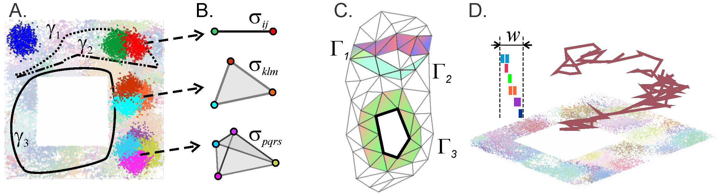
Figure 1: Basic notions of the hippocampal physiology in the context of the topological model. A. In the following, we simulate rat’s navigation in a square-shaped environment $\mathcal{E}$ with a hole in the middle. The curves $\gamma_{1}$, $\gamma_{2}$ and $\gamma_{3}$ represent a few short segments of a physical trajectorynavigated by the rat. The place fields—the regions where the corresponding place cells become active—densely cover the environment, forming a place field map $M_{\mathcal{E}}$. An exemplary place field is represented by a highlighted cluster of blue dots in the top left corner of the environment. The right segment of the environment shows a highlighted pair, a triple and a quadruple of the overlapping place fields; the remaining place fields are dimmed into background. B. Simplexes that correspond to overlapping place fields: a single vertex corresponds to place field (or a single active cell); a link between two vertexes represents a pair of overlapping place fields (or a pair of coactive cells); three overlapping place fields (or a triple of coactive place cells) correspond to a triangle, and so forth. C. A collection of simplexes forms a simplicial complex, which schematically represents the net structure of the place field map. Shown is a fragment of a two-dimensional ($2D$) coactivity complex with simplicial paths $\Gamma_{1}$, $\Gamma_{2}$ and $\Gamma_{3}$ that represent the physical paths $\gamma_{1}$, $\gamma_{2}$ and $\gamma_{3}$ shown on the left. The classes of equivalent simplicial paths describe the topological structure of the coactivity complex: the number of topologically inequivalent, contractible simplicial paths such as $\Gamma_{1}$ and $\Gamma_{2}$, defines the number of pieces, $b_{0}$, of the coactivity complex (Section V). The number of topologically inequivalent paths contractible to a one-dimensional ($1D$) loop defines the number $b_{1}$ of holes and so forth Hatcher . D. A schematic representation of a replayed sequence of place cells, shown over the corresponding place fields. The colored ticks in the top left corner schematically represent a sequence of spikes replayed within a short time window $w$.

2. The topological structure of the coactivity complex provides a convenient framework for representing spatial information encoded by the place cells. For example, the combinations of the cells ignited during the rat’s moves along a physical trajectory $\gamma$, or during a mental replay of such a trajectory, is represented by a “simplicial path”—a chain of simplexes $\Gamma=\{\sigma_{1},\sigma_{2},\ldots,\sigma_{k}\}$ that qualitatively represents the shape of $\gamma$. A simplicial path that loops onto itself represents a closed physical rout; a pair of topologically equivalent simplicial paths represent two similar physical paths and so forth (Fig. 1C).

The net structure of the simplicial paths running through a given simplicial complex $\mathcal{T}$ can be used to describe its topological shape. Specifically, the number of topologically distinct (counted up to topological equivalence) closed paths that contract to zero-dimensional vertexes—the zeroth Betti number $b_{0}(\mathcal{T})$—enumerates the connected components of $\mathcal{T}$; the number of topologically distinct paths that contract to closed chains of links—the first Betti number $b_{1}(\mathcal{T})$—counts its holes and so forth (see Hatcher ; AlexandrovBook and Section V).

3. Dynamics of the coactivity complexes. In practice, the coactivity complexes can be designed to reflect particular physiological properties of the cell assemblies. For example, the time course of the simplexes’ appearance may reflect the dynamics of the cell assemblies’ formation MWind1 ; MWind2 ; PLoZ ; Hoffman , or the details of the place cell activity modulations by the brain waves Arai ; Basso and so on. In particular, a population of forming and disbanding cell assemblies can be represented by a set of appearing and disappearing simplexes, i.e., by a “flickering” coactivity complex $\mathcal{F}$ studied inMWind1 ; MWind2 ; PLoZ . There it was demonstrated that if a cell assembly network rewires sufficiently slowly (tens of seconds to a minute timescale), then the “topological shape” of the corresponding coactivity complex remains stable and equivalent to the topology of the simulated environment $\mathcal{E}$ shown on Fig. 1A, as defined by its Betti numbers $b_{k}(\mathcal{F})=b_{k}(\mathcal{E})=1$, $k=0,1$ (Section V). Physiologically, this implies that cell assemblies’ turnover at the intermediate and the short memory timescales does not prevent the hippocampal network from producing a lasting representation of space, despite perpetual changes of its functional architecture Wang1 .

In particular, the model PLoZ predicts that cell assembly network produces a stable topological map if the connections’ mean lifetime exceeds $\tau\geq 150-200$ secs, which corresponds to the Hebbian plasticity timescale Billeh ; Rakic ; Hiratani ; Russo ; Zenke . For noticeably shorter $\tau$, the topological fluctuations in the simulated hippocampal map are too strong and a stable representation of the environment fails to form. For example, in the case of the place field map shown on Fig. 2A, the connections’ proper lifetime is about $\tau=50$ secs and the corresponding coactivity complex is unstable: its Betti numbers frequently exceed the physical values ($b_{k}(\mathcal{F})>b_{k}(\mathcal{E})$), implying that $\mathcal{F}$ may split into several disconnected pieces, each one of which may contain transient gaps, holes and other topological defects that do not correspond to the physical features of the environment.

For the most time, these defects are scarce ($b_{k}(\mathcal{F})<5$) and may be viewed as topological irregularities that briefly disrupt otherwise functional cognitive map. Indeed, from the physiological perspective, it may be unreasonable to assume that biological cognitive maps never produce topological inconsistencies—in fact, admitting small fluctuations in a qualitatively correct representation of space may be biologically more effective than spending time and resources on acquiring a precise and static connectivity map, especially in dynamically changing environments. However, during certain periods, the topological fluctuations may become excessive, indicating the overall instability of the cognitive map. The origin of such occurrences is clear: if, e.g., the animal spends too much time in particular parts of the environment then the parts of $\mathcal{F}$ that represent the unvisited segments of space begin to deteriorate, leaving behind holes and disconnected fragments (Fig. 2B-D). Outside of these “instability periods,” when the rat regularly visits all segments of the environment, most place cells fire recurrently, thus preventing the coactivity complex $\mathcal{F}$ from deteriorating.

Although this description does not account for the full physiological complexity of synaptic and structural plasticity processes in the cell assembly network, it allows building a qualitative model that connects the animal’s behavior, the parameters describing deterioration of the hippocampal network’s functional architecture and the large-scale topological properties of the cognitive map. This, in turn, provides a context for testing the effects produced by the place cell replays, e.g., their alleged role in acquiring and stabilizing memories by strengthening the connections in parahippocampal networks Sadowski1 ; Sadowski2 ; Colgin . To test these hypotheses, we adopted the topological model PLoZ so that the decaying connections in the simulated hippocampal cell assemblies can be (re)established not only by the place cell activity during physical navigation but also by the endogenous activity of the hippocampal network, and studied the effect of the latter on the structure of the hippocampal map, as outlined below.

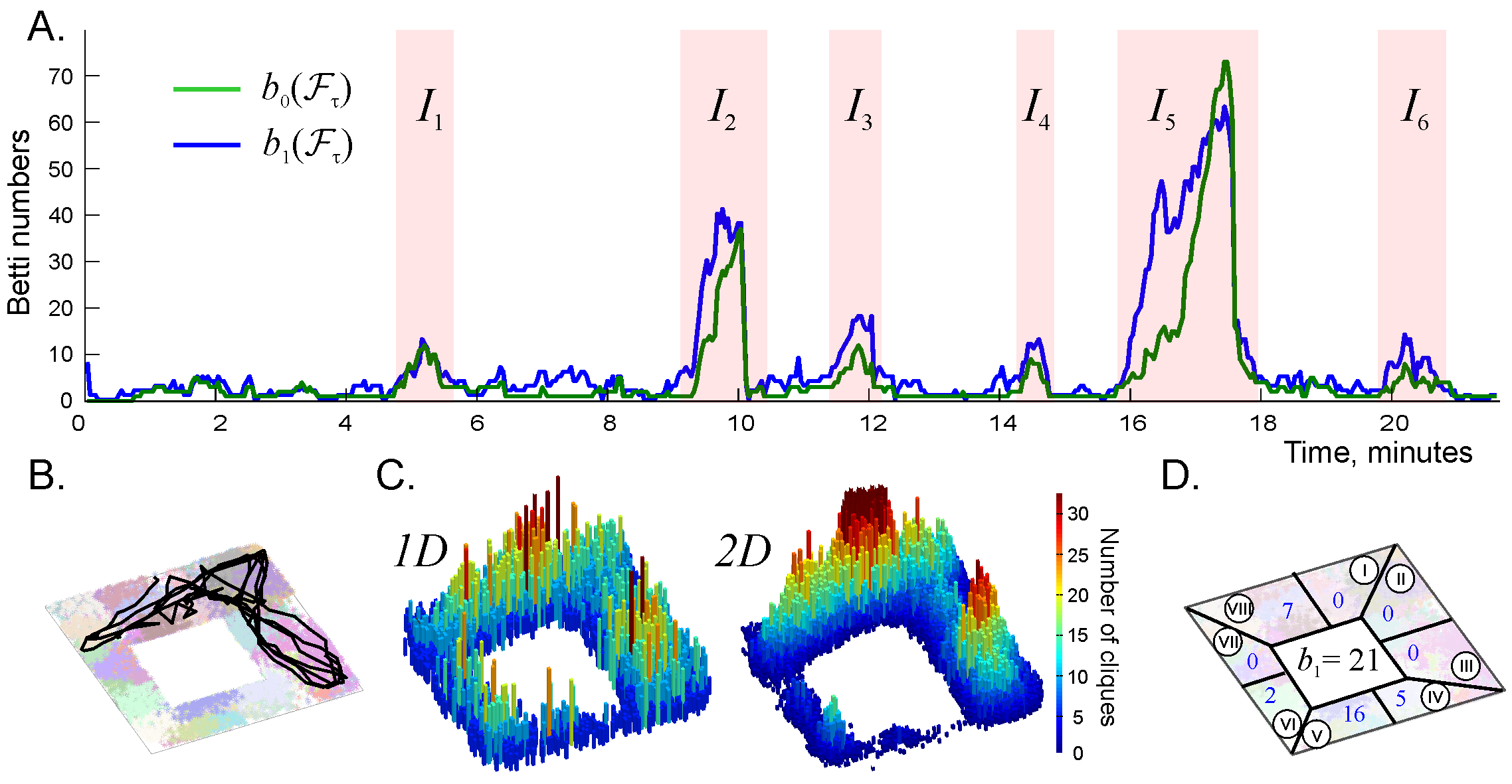
Figure 2: Topological fluctuations in a rapidly decaying coactivity complex in absence of replays. A. The green and the blue lines show, respectively, the zeroth and the first Betti numbers, $b_{0}(\mathcal{F}_{\tau})$ and $b_{1}(\mathcal{F}_{\tau})$ (Section V), as functions of time. For the most time, both Betti numbers remain small, $\langle b_{0}(\mathcal{F}_{\tau})\rangle\approx 2.5$ and $\langle b_{1}(\mathcal{F}_{\tau})\rangle\approx 2.8$, indicating a few disconnected fragments of the coactivity complex $\mathcal{F}_{\tau}$ and a few spurious holes in them. The rapid increase of the Betti numbers during short “instability intervals” $I_{1},\ldots,I_{6}$ (highlighted by pink background) indicate periods of strong topological fluctuations in $\mathcal{F}_{\tau}$. B. A segment of the simulated trajectory taken between the $16$th and $18$th minute shows that the animal spends time before and during the instability period $I_{5}$ in a particular segment of the arena. During this time, the connections over the unvisited segments of $\mathcal{E}$ start to decay (here the connections’ mean lifetime is $\tau=50$ sec), as a result of which the coactivity complex $\mathcal{F}_{\tau}$ fractures into a large number of disconnected pieces riddled in holes, which explains the splash of $b_{0}(\mathcal{F}_{\tau})$ and $b_{1}(\mathcal{F}_{\tau})$. C. Spatial histograms of the links (i.e., centers of the pairwise place field overlaps, left panel) and of the three-vertex simplexes (i.e., centers of triple place field overlaps, right panel) present in $\mathcal{F}_{\tau}$ during the instability period $I_{5}$. The simplexes concentrate over the northeast corner of the environment, whereas the populations of simplexes over the south and the southwestern parts thin out. D. The “local” Betti number $b_{1}$ (blue numerals) computed separately for the eight sectors of the environment (encircled Roman numerals) indicate that the holes emerge in all the “abandoned” parts, e.g., sector IV contains 5 holes and sector V contains 16 holes, etc. The global Betti number computed at about 16th minute for the entire complex, $b_{1}(\mathcal{F}_{\tau})=21$, is shown in the middle.

4. The implementation of the coactivity complexes is based on a classical model of the hippocampal network, in which place cells $c_{i}$ are represented as vertexes $v_{i}$ of a “cognitive graph” $\mathcal{G}$, while the connections between pairs of coactive cells are represented by the links, $\varsigma_{ij}=[v_{i},v_{j}]$ of this graph Burgess ; Muller ; SchemaS . The assemblies of place cells $\varsigma=[c_{1},c_{2},\ldots,c_{n}]$—the “graphs of synaptically interconnected excitatory neurons,” according to Syntax —then correspond to fully interconnected subgraphs of $\mathcal{G}$, i.e., to its maximal cliques Hoffman ; CAs ; SchemaS . Since each clique $\varsigma$, as a combinatorial object, can be viewed as a simplex spanned by the same set of vertexes (see Suppl. Fig. 6 in Basso ), the collection of cliques of the graph $\mathcal{G}$ defines a clique simplicial complex Jonsson , which proves to be is one of the most successful implementations of the coactivity complex. In previous studies Basso ; Hoffman ; CAs ; SchemaS , we demonstrated that in absence of decay ($\tau=\infty$), such a complex $\mathcal{T}$ effectively accumulates information about place cell coactivity at various timescales, capturing the correct topology of planar and voluminous environments. If the decay of the connections is taken into account ($\tau<\infty$), then the topology of the “flickering” coactivity complex $\mathcal{F}$ remains stable for sufficiently small rates, but if $\tau$ becomes too small, the topology of $\mathcal{F}$ may degrade. A question arises, whether the replays can slow down its deterioration, as the biological considerations suggest.

5. Dynamics of the coactivity graph. Physiologically, place cell spiking is synchronized with the components of the extracellular local field potential—the so-called brain waves that also define the timescale of place cell coactivity BuzsakiBook . Specifically, two or more place cells are considered coactive, if they fire spikes within two consecutive $\theta$-cycles—approximately 150-250 msec interval Mizuseki —a value that is also suggested by theoretical studies Arai . In the following, this period will define the shortest timescale at which the functional connectivity of the simulated hippocampal network can change. For example, a new link $\varsigma_{ij}=[v_{i},v_{j}]$ in the coactivity graph will appear, if a coactivity of the cells $c_{i}$ and $c_{j}$ was detected during a particular $2\theta$ period. In absence of coactivity, the links can also disappear with probability

$$p_{0}(t)=\frac{1}{\tau}e^{-t/\tau},$$ (1)

where $t$ is the time measured from the moment of last spiking of both cells $c_{i}$ and $c_{j}$ and the parameter $\tau$ defines the mean lifetime of the synaptic connections in the cell assembly network. In the following, $\tau$ will be the only parameter that describes the deterioration of the synaptic connections within the cell assemblies PLoZ . We will therefore use the notations $\mathcal{G}_{\tau}$ and $\mathcal{F}_{\tau}$ to refer, respectively, to the flickering coactivity graph with decaying connections and to the resulting flickering coactivity complex with decaying simplexes.

6. Replays of place cell sequences may in general represent both spatial and nonspatial memories. In the following, we simulate only spatial replays by constructing simplicial paths that represent previously navigated trajectories. Specifically, we select chains of connections that appeared in the coactivity graph $\mathcal{G}_{\tau}$ at the initial stages of navigation, and reactivate them at the later replay times $t_{r}$, $r=1,2,\ldots,N_{r}$ Kudrimoti ; ONeill1 . To replay a trajectory originating at a given timestep $t_{i}$, we randomly select a coactivity link $\varsigma_{kl}^{(i)}\in\mathcal{G}_{\tau}(t_{i})$ that is active within that time window; this link is then gives rise to a sequence of joined links, randomly selected among the ones that activate at the consecutive time steps, $\varsigma_{lm}^{(i+1)},\varsigma_{mn}^{(i+2)},\ldots$. Since there are typically several active links at every moment, this procedure allows generating a large number of replay trajectories. The physiological duration of replays—typically about 100-200 msec Colgin —roughly corresponds to the coactivity window widths, i.e., to the timesteps in which the coactivity graph evolves; we therefore “inject” the activated links into a particular coactivity window $t_{r}$ in order to simulate rapid replays.

After a simplicial trajectory is replayed, the injected links begin to decay and to (re)activate in the course of the animal’s moves across the environment, just as the rest of the links. Most of these “reactivated” links simply rejuvenate the existing connections in $\mathcal{G}_{\tau}$. However, some injections instantaneously reinstate decayed connections and produce an additional population of higher order cliques, which affect the topological properties of the coactivity complex $\mathcal{F}_{\tau}$, and hence—according to the model—of the cognitive map. As mentioned previously, hippocampal replays are believed to enable spatial learning by stimulating inactive connections, by slowing down their decay and by reinforcing cell assemblies’ stability Carr ; Jadhav1 ; Sadowski2 ; Ego ; Girardeau1 ; Girardeau2 . In the model’s terms, this hypothesis translates as follows: the additional influx of rejuvenated simplexes provided by the replays should qualitatively improve the topological structure of the flickering coactivity complex, slow down deterioration of its simplexes, suppress its topological defects and in general help to sustain its topological integrity. In the following, we test this hypothesis by simulating different patterns of the place cell reactivations and quantifying the effect that this produces on the simulated cognitive map.

III Results

1. Initial testing. The effect produced by the replays on the cognitive map depends on the parameters of the model: the selection of replayed trajectories, the injection times, the frequency of the replays and so forth. To start the simulations, we selected $N_{s}=80$ different replay sequences originating at $N_{i}=25$ moments of time, $t_{i}$, $i=1,\ldots,N_{i}$, between $20$ and $200$ seconds of navigation (the initial interval $I_{init}$). During this period, the trajectory covers the arena more or less uniformly: a typical $25$ secs long segment of a trajectory extends across the entire the environment and contains on average about $l_{s}=100$ links (Fig. S1). As a result, the corresponding simplicial paths traverse the full coactivity complex $\mathcal{F}_{\tau}$ and one would expect that replaying these paths should help to suppress the topological defects in $\mathcal{F}$. To verify this prediction, we replayed the resulting pool of $\mathcal{G}$-link sequences within the main instability period $I_{5}$ using different approaches and tested whether this can suppress the topological fluctuation (Fig. 3A).

In the first scenario, all replay chains were injected into the connectivity graph $\mathcal{G}_{\tau}$ at once, in the middle of the instability period $I_{5}$ (Fig. 3B). As a result of such a “massive” instantaneous replay, the topological fluctuations are initially suppressed but then they quickly rebound, producing about the same number of spurious $0D$ loops (i.e., the cognitive map remains as fragmented as before) and an even higher number of $1D$ loops that mark spurious holes in the cognitive map (Suppl. Movie 1). In other words, our model suggests that a single “memory flash” fails to correct the deteriorating memory map even at a short timescale, which suggests that more regular replay patterns are required.

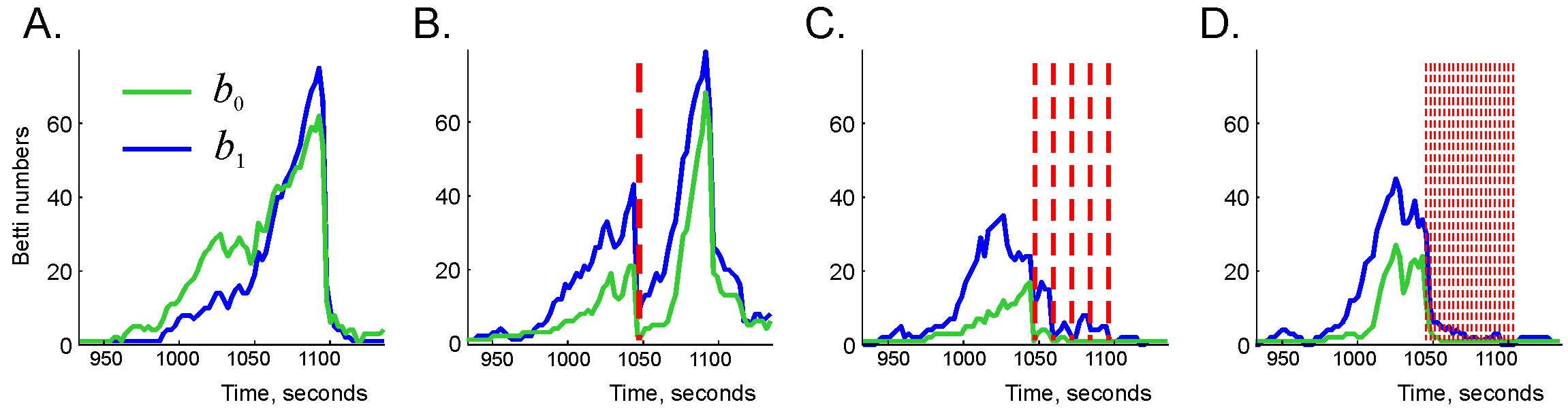
Figure 3: Suppressing topological fluctuations by reactivation of simplexes. A. During the instability period $I_{5}$ (approximately between 15.5 and 18.5 mins) the topological fluctuations in the coactivity complex become very strong, with the Betti numbers soaring at $b_{0}(\mathcal{F}_{\tau})\approx 65$ and $b_{1}(\mathcal{F}_{\tau})\approx 75$. B. If all the reactivated links are injected into the coactivity complex at once, at a moment preceding the peak of the Betti numbers (marked by a vertical red dashed line), the fluctuations in the coactivity complex are immediately suppressed. However, as the connection decay takes over, the fluctuations kick back, reaching the original high values in under a minute. C. Five consecutive replays, marked by five vertical red dashed lines, produce a more lasting effect, reducing the Betti numbers to smaller values $\langle b_{0}(\mathcal{F}_{\tau})\rangle\approx 3$ and $\langle b_{1}(\mathcal{F}_{\tau})\rangle\approx 7$ over the remainder of the instability period. D. More frequent replays (once every $2.5$ secs, vertical dashed lines) nearly suppress the topological fluctuations, producing the average values $\langle b_{0}(\mathcal{F}_{\tau})\rangle\approx 1.2$ and $\langle b_{1}(\mathcal{F}_{\tau})\rangle\approx 3$, i.e., leaving only a couple of spurious loops in $\mathcal{F}_{\tau}$.

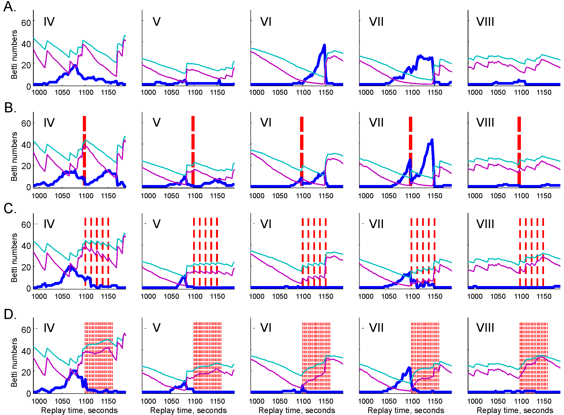
Figure S2: Local topological fluctuations. A. The first Betti number, $b_{1}$ (thick blue line) computed for the sectors IV-VIII of the environment, enumerated according to Fig. 2D. The changes in numbers of cliques and in Betti numbers over the segments I, II and III are insignificant and are not shown. The blue and the magenta lines represent the numbers of pair and triple connections, $N_{2}(\mathcal{F}_{\tau})$ and $N_{3}(\mathcal{F}_{\tau})$, scaled down by the factors $10^{-3}$ and $10^{-4}$ respectively, to fit into the panels. Prior to the instability period, the numbers of $N_{3}(\mathcal{F}_{\tau})$ and $N_{2}(\mathcal{F}_{\tau})$ decrease, indicating that the coactivity complex $\mathcal{F}_{\tau}$ thins out, which also produces an increasing number of spurious topological loops. In contrast, the increase of the local Betti numbers $b_{1}$ stops when the connections start to accumulate, i.e., when the decay of the coactivity simplexes is counterbalanced by their regular reactivation due to the rat’s uniform sampling of the environment. B. In the case of instantaneous massive replay (memory flash, time marked by the vertical red dashed line), the increase of $b_{1}$ is briefly halted over all segments of the environment, but then it restarts at the same rate. C. For a more frequent replays ($N_{r}=5$, times marked by the five red vertical dashed lines), spurious loops are suppressed in all sectors, most effectively over the sectors VI and VII. D. In the case of a more regular replay ($N_{r}=20$ vertical dashed lines), spurious loops are effectively terminated in all sectors over the entire instability period.

Indeed, if the same set of replay sequences is uniformly distributed into $N_{r}=5$ consecutive groups inside the instability period $I_{5}$ (one group per 36 seconds, $N_{s}/N_{r}=16$ chains of links each), then the topological fluctuations in the coactivity complex $\mathcal{F}_{\tau}$ subside more and over a longer period (see Fig. 3C and Suppl. Movie 2). If the replays are produced even more frequently (every 9 seconds, i.e., about 20 replays total, $N_{s}/N_{r}\approx 4$ chains of links injected per replay) then the topological fluctuations in $I_{5}$ are essentially fully suppressed over the entire environment (Fig. 3D, Fig. S2 and Suppl. Movie 3).

One can draw two principal observations from these results: first, that spontaneous reactivation of connections at the physiological timescale can qualitatively alter the topological structure of the flickering coactivity complex and second, that the temporal pattern of replays plays a key role in suppressing the topological fluctuations in the cognitive map.

2. Implementation of the replays. Electrophysiological data shows that the frequency of the replays ranges between $0.1$ Hz in active navigation to $0.4$ Hz in quiescent states and $4$ Hz during sleep ONeill1 ; Colgin ; Jadhav1 ; Sadowski2 . Since we model spatial learning taking place during active navigation, we implemented replays at the maximal rate of $0.4$ Hz, which corresponds to no more than one replay event over ten consecutive coactivity intervals. Second, we took into account the fact that, in complex environments, hippocampus may replay a few sequences simultaneously. For example, on the $Y$-track ONeill1 two simultaneous replay sequences can represent the two prongs of the $Y$. In open environments, there may be more simultaneously replayed sequences; however we used the most conservative estimate and replayed two different sequences at each replay moment $t_{r}$.

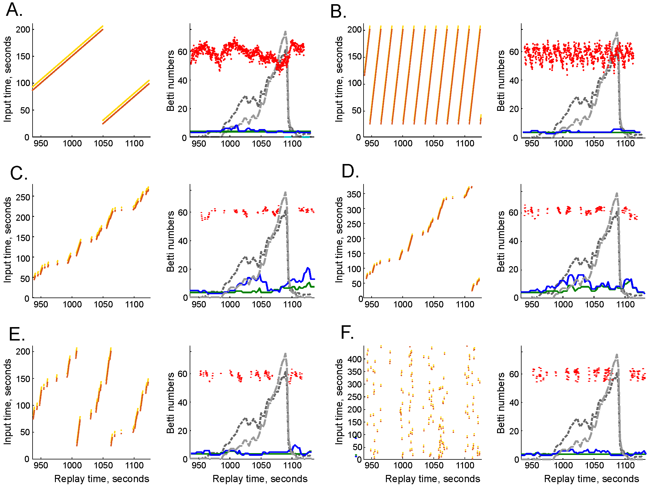
Figure 4: Suppressing the topological fluctuations by replays. In all cases, the injection diagram on the left relates the times when the place cell sequences were originally produced (vertical axis) to the times when they are replayed (horizontal axis). Each yellow and brown dot corresponds to a replayed sequence. On the right panel, the replay times are marked by red dots, with the vertical scatter proportional to the simulated speed of the animal. The resulting zeroth Betti number ($b_{0}(\mathcal{F}_{\tau})$, green line) and the first Betti number ($b_{1}(\mathcal{F}_{\tau})$, blue line) are shown in the foreground, and the original, unstable Betti numbers (without replays) are shown in the background (dark and light dashed gray lines, respectively). A. A simple translational replay of a couple of sequences repeated over a three minute period (between $20$ and $200$ secs), with a $\Delta T=14$ min delay. The zeroth Betti number regains its physical value, $b_{0}(\mathcal{F}_{\tau})=b_{0}(\mathcal{E})=1$, indicating that cognitive map reconnects into one piece. The first Betti number fluctuates near the physical value $b_{1}(\mathcal{F}_{\tau})=1.5\pm 2.2$, indicating that nearly all spurious holes are closed. B. Compressed replay: a three-minute period is replayed repeatedly over several consecutive $20$ sec intervals. Here the zeroth Betti number remains correct, $b_{0}(\mathcal{F}_{\tau})=1$, and the fluctuations of the first Betti number reduce farther, $b_{1}(\mathcal{F}_{\tau})=1.2\pm 1$. C. Modulating the replay times by slow move periods ($v<15$ cm/sec) produces sparser replays. As a result, the topological fluctuations in the case of uncompressed, speed-modulated delayed replays increase, $b_{0}(\mathcal{F}_{\tau})=4.2\pm 1.9$, $b_{1}(\mathcal{F}_{\tau})=8.2\pm 3.4$. D. Small compressions (up to $300$ seconds replayed over $\sim 150$ second period, same delay) may intensify the fluctuations: $b_{0}(\mathcal{F}_{\tau})=5.9\pm 2.4$, $b_{1}(\mathcal{F}_{\tau})=9.2\pm 4.1$. E. Further compression of the replays improves the results, $b_{0}(\mathcal{F}_{\tau})=1.1\pm 1.4$, $b_{1}(\mathcal{F}_{\tau})=1.7\pm 2$, although the variations of $b_{1}(\mathcal{F}_{\tau})$ remain high compared to the cases in which the replays are not modulated by the speed. F. Random replays reduce the fluctuations even further: the coactivity complex acquires the correct zeroth Betti number $b_{0}(\mathcal{F}_{\tau})=1$ (the map becomes connected), producing occasional spurious loops, $b_{1}=1.4\pm 1.2$—occasional topological irregularities.

In the simplest scenario, we injected pairs of sequences into the coactivity graph $\mathcal{G}_{\tau}$ with a constant delay of about $\Delta T=t_{i}-t_{r}\approx 14$ minutes after their physical onset, which placed them inside of the instability period $I_{5}$ (Fig. 4A). In response, the topological fluctuations in the coactivity complex $\mathcal{F}_{\tau}$ significantly diminished. In fact, the zeroth Betti number (the number of the disconnected components) regained its physical value $b_{0}(\mathcal{F}_{\tau})=1$, indicating that the replays helped to pull the fragments of the cognitive map together into a single connected piece. The first Betti number (the number of holes) remains on average close to its physical value, $\langle b_{1}(\mathcal{F}_{\tau})\rangle=1.5$, exhibiting occasional fluctuations, $\Delta b_{1}=\pm 2.2$.

As mentioned above, the occasional islets separating from the main body of the simplicial complex or a few small holes appearing in it for a short period should be viewed as topological irregularities, rather than signs of topological instability. We therefore base the following discussion on addressing only the qualitative differences produced by the replays on the topology of the cognitive map: whether replays can prevent fracturing of the complex into multiple pieces and rapid proliferation of spurious loops in all dimensions. From such perspective, our results demonstrate that translational replays at a physiological rate can effectively restore the correct topological shape of the cognitive map, which illustrates functional importance of the replay activity.

Since the replays are generated by the endogenous activity of the hippocampal network, the relative temporal order of the replayed sequences can be altered, i.e., the replay times $t_{r}$ can be spread wider or denser than their “physical” origination times $t_{i}$. The effect of the replays will be, respectively, weaker or stronger than in the case of translational delay, due to the corresponding changes of the sheer number of the reactivated links. However, one can factor out the direct contribution of the replays’ volume and study more subtle effects produced specifically by the replay’s temporal organization. To this end, we split the replay period $I_{5}$ into a set of $N_{R}$ shorter subintervals, $I^{1}_{5},I^{2}_{5},\ldots I^{N_{R}}_{5}$, and then replayed the sequences of links originating from the initial three minute interval $I_{init}$ within each subinterval $I^{n}_{5}$, $n=1,2,\ldots,N_{R}$. Since only two sequences are replayed within every coactivity window, the total number of the (re)activated sequences remains the same as in the delayed replay case, even though the source interval $I_{init}$ is compressed $N_{R}$-fold in time. Thus, the difference between the effects produced by the “compressed” replays will be due solely to the differences in their temporal reorganizations.

The results illustrated on Fig. 4B demonstrate that the compressed replays suppress the topological fluctuations more effectively. For example, the repeated replay in a sequence of 20 sec intervals ($N_{R}=9$ fold compression) not only restores the correct value of the zeroth Betti number, $b_{0}(\mathcal{F}_{\tau})=1$, but also drives the average number of noncontractible simplicial loops close to physical value, $\langle b_{1}(\mathcal{F}_{\tau})\rangle=1.2\pm 1$. In other words, $\mathcal{F}_{\tau}$ almost regains its topologically correct shape, with an occasional spurious hole appearing for less than a second. Physiologically, these results suggest that time-compressed, repetitive “perusing” through memory sequences helps to prevent deterioration of global memory frameworks better than simple “orderly” recalls.

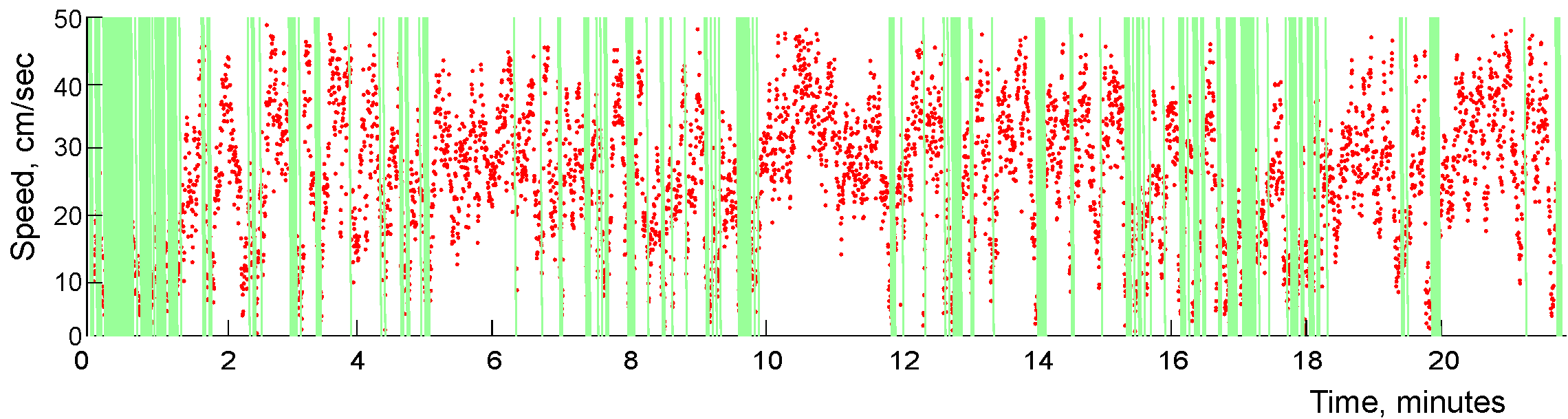
Figure S3: Speed modulation of the replays. The red dots mark the mean values of the animal’s speed during the coactivity windows—the potential replay times. The green lines mark the slow motion periods, $v<15$ cm/sec, occurring during $14\%$ of time—the replay windows.

3. Speed modulation of the replays. Since replays are mostly observed during quiescent periods and slow moves ONeill1 ; ONeill2 , we studied whether such “low-speed” replays will suffice for suppressing the topological fluctuations in the cognitive map. Specifically, we identified the periods when the speed of the animal falls below $15$ cm/sec (which, in our simulations happens during $14\%$ of time, see Fig. S3 and Nadasdy ; Koene ), and replayed the place cell sequences only during these periods.

It turns out that although the resulting slow motion replays can stabilize the topological structure of the simulated cognitive map, the effect strongly depends on their temporal organization. Specifically, in the simple delayed replay scenario, the topological fluctuations remain significantly higher than without speed modulation (Fig. 4C, Suppl. Movie 4). On average, the coactivity complex contains about a dozen of spurious loops: it remains split in a few pieces, $\langle b_{0}(\mathcal{F}_{\tau})\rangle=4.2$, that together contain $\langle b_{1}(\mathcal{F}_{\tau})\rangle=8.2$ holes on average. This is a natural result—one would expect that speed restrictions will diminish the number of the injected active connections and hence that $\mathcal{F}_{\tau}$ will degrade more. A slightly compressed replay (4 minutes of activity replayed over 3 minute period) does not improve the result: both the number of disconnected components and the number of holes in them increase $\langle b_{0}(\mathcal{F}_{\tau})\rangle=5.9$, $\langle b_{1}(\mathcal{F}_{\tau})\rangle=9.2$ (Fig. 4D). However, if the replays are compressed further, the average number of disconnected components is significantly reduced: for the threefold compression shown on Fig. 4E, the mean values are $\langle b_{0}(\mathcal{F}_{\tau})\rangle=1.1$ and $\langle b_{1}(\mathcal{F}_{\tau})\rangle=1.7$, i.e., the encoded map approaches the quality of the maps produced with unrestricted replays.

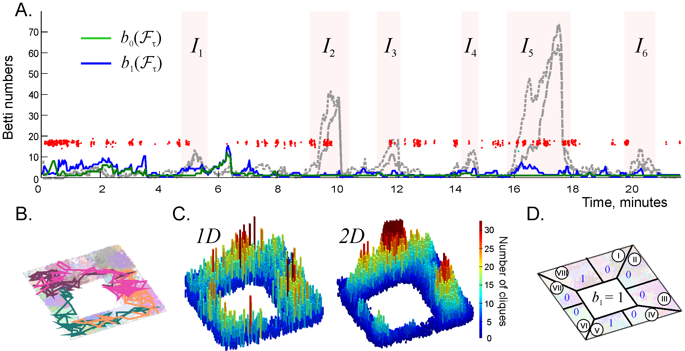
Figure 5: Replays suppress topological fluctuations over the entire navigation period. A. The time dependence of the Betti numbers $b_{0}(\mathcal{F}_{\tau})$ and $b_{1}(\mathcal{F}_{\tau})$ (the green and the blue line respectively) in presence of the replays. The topological fluctuations that previously overwhelmed the map during the “instability intervals” (shown in the background by two dashed gray lines, see Fig. 2A) are now nearly fully suppressed. The replay moments, $t_{r}$, marked by the red dots, are modulated by speed, $v<15$ cm/sec. B. Several examples of replayed trajectories over the navigated environment are shown in different colors (see also Fig. S1). C. Spatial histograms of the centers of the links (left panel) and of the three-vertex simplexes (right panel) during the instability period $I_{5}$ in presence of the replays. The populations of simplexes over the south and the southwestern parts of the environment in presence of the replays have increased compared to the case shown on Fig. 2C, which suppresses spurious topological loops in the coactivity complex. D. The Betti numbers $b_{1}$ computed for the eight sectors of the environment are also significantly reduced, indicating that the topological fluctuations are suppressed both locally and globally. The deviations of $b_{1}$ from 0 in the sectors V and VIII are due to boundary effects at the sector’s edges that do not affect the global value $b_{1}(\mathcal{F}_{\tau})=1$. All zeroth Betti numbers, both local and global, assume correct values $b_{0}=1$ and are not shown.

The effectiveness of the latter scenario can be explained by noticing that replay compression brings the activities that are widely spread in physical time into close temporal vicinities during the replays. In other words, in compressed replays, a wider variety of connections is activated at each $t_{r}$: the real-time separation between activity patterns shrinks. This helps to reduce or eliminate the temporal “lacunas” in place cell coactivity across the entire hippocampal network and hence to prevent spontaneous deterioration of its parts. In physiological terms, this implies that the compressed replays of the place cell patterns are less constrained by the physical temporal scale of the rat’s navigational experiences, which leads to a more even activation of the connections in the network and helps to prevent the memory map’s fragmentation.

To test this idea, we amplified this effect by shuffling the order of the replayed sequences and by randomizing the injection diagram, thus enforcing a nearly uniform pattern of injected activity across the simulated population of cell assemblies. This indeed proved to be the most effective replay strategy: as shown on Fig. 4F, such replay patterns restore the topological shape of the coactivity complex, allowing only occasional holes: $\langle b_{0}(\mathcal{F}_{\tau})\rangle=1$, $\langle b_{1}(\mathcal{F}_{\tau})\rangle\approx 1.4\pm 1.2$ (Suppl. Movie 5). Thus, the model suggests that “reshuffling” the temporal sequence of memory replays helps to sustain memory framework better than orderly recollections, occurring in natural past-to-future succession. The effect of random replays of the place cell sequences over the entire simulated navigation period shown on Fig. 5 clearly illustrates the importance of replays for rapid encoding of topological maps: the fluctuations in the cognitive map are uniformly suppressed.

IV Discussion

The model discussed above suggests that replays of place cell activity help to learn and to sustain the topological structure of the cognitive map. The physiological accuracy of the replay simulation can be increased ad infinitum, by incorporating more and more parameters into the model. In this study we use only a few basic properties of the replays, which, however, capture several key functional aspects of the replay activity. First, the model implements an effective feedback loop, in which the onset of topological instabilities in the flickering coactivity complex $\mathcal{F}_{\tau}$ triggers the replays that restore its integrity. Indeed, the cell assemblies’ (and the corresponding simplexes’) decays intensify as the animal’s exploratory movements slow down and visits to particular segments of the environment become less frequent. On the other hand, low speed periods define temporal windows during which the simulated replays are injected into the network, which work to suppress the topological instabilities. Second, the model allows controlling the replays’ temporal organization independently from the other parameters or neuronal activity and exploring the replays’ contribution into acquiring and stabilizing the cognitive maps. The results demonstrate that in order to strengthen the decaying connections in the hippocampal network effectively, the replays must 1) be produced at a sufficiently high rate that falls within the physiological range and 2) distribute without temporal clustering, in a semi-random order.

An important aspect of the obtained results is a separation of the timescales at which different types of topological information is processed. On the one hand, rapid turnover of the information about local connectivity at the working memory timescale is represented by quick recycling of the cell assemblies and rapid spontaneous replays of the learned sequences. On the other hand, the large-scale topological structures of the cognitive map, described by the instantaneous homological characteristics of the coactivity complex, emerge at the intermediate memory timescale. Thus, the model suggests that the characteristic timescale of the topological loops’ dynamics is by an order of magnitude larger than the timescale of fluctuations at the cell assembly level. This observation provides a functional perspective on the role played by the place cell replays in learning: by reducing the fluctuations, replays help separating the fast and the slow information processing timescales and hence to extract stable topological information that can be used to build a long-term, qualitative representation of the environment. This separation of timescales corroborates with the well-known observation that transient information is rapidly processed in the hippocampus and then the resulting memories are consolidated and stored in the cortical areas, but at slower timescales and for longer periods.

V Methods

Topological Glossary.

For the reader’s convenience, we briefly outline the key topological terms and concepts used in this paper.

$\bullet$ An abstract simplex of order $d$ is a set of $(d+1)$ elements, e.g., a set of coactive cells, $\sigma^{(d)}=[c_{i_{0}},c_{i_{1}},\ldots,c_{i_{d}}]$ or a set of place fields, $\sigma^{(d)}=[\upsilon_{j_{0}},\upsilon_{j_{1}},\ldots,\upsilon_{j_{k}}]$. The subsets of $\sigma^{(d)}$ are its subsimplexes. Subsimplexes of maximal dimensionality $(d-1)$ are referred to as facets of $\sigma^{(d)}$.

$\bullet$ An abstract simplicial complex $\Sigma$ is a family of abstract simplexes closed under the overlap relation: a nonempty overlap of any two simplexes $\sigma^{(d_{1})}_{1}\in\Sigma$ and $\sigma^{(d_{2})}_{2}\in\Sigma$ is a subsimplex of both $\sigma^{(d_{1})}_{1}$ and $\sigma^{(d_{2})}_{2}$.

$\bullet$ Geometrically, simplexes can be visualized as $d$-dimensional polytopes: $\sigma^{(0)}$ as a point, $\sigma^{(1)}$ as a line segment, $\sigma^{(2)}$ as a triangle, $\sigma^{(3)}$ as a tetrahedron, etc. The corresponding geometric simplicial complexes are multidimensional polyhedra that have a shape and a structure that does not change with simplex deformations, e.g., disconnected components, holes, cavities of different dimensionality, etc. This structure, commonly referred to as topological AlexandrovBook , is identical in a geometric simplicial complex to and in the abstract complex built over the vertexes of the geometric simplexes. Thus, abstract simplicial complexes may be viewed as structural representations of the conventional geometric shapes.

$\bullet$ Topological properties of the simplicial complexes are established based on algebraic analyses of chains, cycles and boundaries.

A chain $\alpha^{(d)}$ is a formal combination $d$-dimensional simplexes with coefficients from an algebraic ring or a field. Intuitively, they can be viewed, e.g., as the simplicial paths described in Section II. Such combinations permit algebraic operations: they can be added, subtracted, multiplied by a common factor, etc. As a result, the set of all chains of a given simplicial complex, $C(\Sigma)$, also forms an algebraic entity, e.g., if the chains’ coefficients form to a field, then $C(\Sigma)$ forms a vector space.

A boundary of a chain, $\partial\alpha^{(d)}$, is a formal combination of all the facets of the $\alpha$-chain, with the coefficients inherited from $\alpha$ and alternated so that the boundary of $\partial\alpha^{(d)}$ vanishes, $\partial^{2}\alpha^{(d)}=0$. This universal topological principle—boundary of a boundary is a null set—can be illustrated on countless examples, e.g., by noticing that the external surface of a triangular pyramid $\sigma^{(3)}$—its geometric boundary—has no boundary itself.

Cycles generalize the previous example—a generic cycle $z$ is a chain without a boundary, $\partial z=0$. Intuitively, cycles correspond to agglomerates of simplexes (e.g., simplicial paths) that loop around holes and cavities of the corresponding dimension. Note however, that although all boundaries are cycles, not all cycles are boundaries.

$\bullet$ Homologies. Two cycles, $z_{1}$ and $z_{2}$, are equivalent, or homologous, if they differ by a boundary chain. The set of equivalent cycles forms a homology class. If the chain coefficients come from a field, then the homology classes of $d$-dimensional cycles form a vector space ${\sf H}_{d}(\Sigma)$. The dimensionality of this vector space is the $d$-th Betti number of the simplicial complex $\Sigma$, $b_{d}(\Sigma)=\dim{\sf H}_{k}(\Sigma)$, which counts the number of independent $d$-dimensional holes in $\Sigma$.

$\bullet$ Flickering complexes $\mathcal{F}(t)$ consist of simplexes that may disappear or (re)appear, so that the complex as a whole may grow or shrink from one moment to another (see Fig.2 in PLoZ ),

$$\mathcal{F}(t_{1})\subseteq\mathcal{F}(t_{2})\subseteq\mathcal{F}(t_{3})\supseteq\mathcal{F}(t_{4})\subseteq\mathcal{F}(t_{5})\supseteq\ldots.$$

Computing the corresponding Betti numbers, $b_{k}(\mathcal{F}(t))$, requires a special technique—Zigzag persistent homology theory that allows tracking cycles in $\mathcal{F}$ on moment-to-moment basis Carlsson2 ; Carlsson3 ; PLoZ .

$\bullet$ A clique in a graph $G$ is a set of fully interconnected vertices, i.e., a complete subgraph of $G$. Combinatorially, cliques have the same key property as the abstract simplexes: any subcollection of vertices in a clique is fully interconnected. Hence a nonempty overlap of two cliques $\varsigma$ and $\varsigma^{\prime}$ is a subclique in both $\varsigma$ and $\varsigma^{\prime}$, which implies that cliques may be formally viewed as abstract simplexes and a collection of cliques in a given graph $G$ produces its clique simplicial complex $\Sigma(G)$ Jonsson . In particular, the clique coactivity complexes $\mathcal{T}_{\varsigma}$ is induced from the coactivity graphs $\mathcal{G}$ Basso ; Hoffman ; CAs and the flickering clique complexes $\mathcal{F}_{\tau}$ are constructed using coactivity graph with flickering connections $\mathcal{G}_{\tau}$, MWind1 ; MWind2 ; PLoZ . Note however, that the topological analyses address the topology of the coactivity complexes, rather than the network topology of $\mathcal{G}$.

Spike simulations.

The environment shown on Fig. 1A is simulated after typical arenas used in typical electrophysiological experiments. Over the navigation period $T_{tot}=30$ min, the trajectory covers the environment uniformly. The maximal speed of the simulated movements is $v_{\max}=50$ cm/sec, with the mean value $\bar{v}=25$ cm/sec. The firing rate of a place cell $c$ is defined by

$$\lambda_{c}(r)=f_{c}e^{-\frac{(r-r_{c})^{2}}{2s^{2}_{c}}}$$

where $f_{c}$ is the maximal firing rate and $s_{c}$ defines the size of the place field centered at $r_{c}$ Barbieri . In addition, spiking is modulated by the $\theta$-oscillations—-a basic cycle of the extracellular local field potential in the hippocampus, with the frequency of about $8$ Hz Arai ; Mizuseki ; Huxter . The simulated ensemble contains $N_{c}=300$ virtual place cells, with the typical maximal firing rate $f=14$ Hz and the typical place field size $s=20$ cm.

VI Acknowledgments

The work was supported by the NSF 1422438 grant.

VII References

SUPPLEMENTARY FIGURES

Figure S1: Replayed trajectories. Eight simulated trajectories of length $l_{s}=100$, which corresponds to about $25$ secs of of physical time, extending across different segments of the environment. The positions of the replayed trajectories over the environment are not related to the location of the rat at the moment when the replays occurred.

SUPPLEMENTARY MOVIE CAPTIONS

Suppl. Movie 1. Single replay. First two panels show the dynamics of the spatial histograms of the two-vertex and the three-vertex simplexes (i.e., centers of the pairwise and the triple overlaps between place fields) present in $\mathcal{F}_{\tau}$. The right panel shows the trajectory (green line) in the square environment split into eight segments (see Fig. 2C,D). The numbers in each segment $S_{i}$ represent the pair local Betti numbers $(b_{0}(S_{i}),b_{1}(S_{i}))$ and the pair of the global Betti number $(b_{0}(\mathcal{E}),b_{1}(\mathcal{E}))$ are shown in the center. Around $t=24$ secs, a large number of replayed sequences is injected (see Fig. 3B). The topological fluctuations are instantaneously suppressed but then they immediately restart and reach back to high values.

Suppl. Movie 2. Five replays suppress the topological fluctuations better (Fig. 3C).

Suppl. Movie 3. Twenty replays (about one replay in every 9 seconds) nearly extinguish the topological fluctuations during the instability period (Fig. 3D).

Suppl. Movie 4. Additional speed-modulation revives topological fluctuations (Fig. 4C,D).

Suppl. Movie 5. Speed-modulated, randomized replays restore the correct topological shape of the map (Fig. 4F).

References

- (1) Johnson A, Redish AD (2007) Neural Ensembles in CA3 Transiently Encode Paths Forward of the Animal at a Decision Point. J. Neurosci., 27: 12176-12189.
- (2) Pastalkova E, Itskov V, Amarasingham A, Buzsaki G (2008) Internally generated cell assembly sequences in the rat hippocampus. Science 321: 1322-1327.
- (3) Wilson MA, McNaughton BL (1994) Reactivation of hippocampal ensemble memories during sleep. Science 265: 676-679.
- (4) Louie K, Wilson MA (2001) Temporally Structured Replay of Awake Hippocampal Ensemble Activity during Rapid Eye Movement Sleep. Neuron 29: 145-156.
- (5) Ji D, Wilson MA (2007) Coordinated memory replay in the visual cortex and hippocampus during sleep. Nat Neurosci 10: 100-107.
- (6) Papale AE, Zielinski MC, Frank LM, Jadhav SP, Redish AD Interplay between Hippocampal Sharp-Wave-Ripple Events and Vicarious Trial and Error Behaviors in Decision Making.Neuron 92: 975-982.
- (7) Foster DJ, Wilson MA (2006) Reverse replay of behavioural sequences in hippocampal place cells during the awake state. Nature 440: 680-683.
- (8) Hasselmo ME (2008) Temporally structured replay of neural activity in a model of entorhinal cortex, hippocampus and postsubiculum. Eur J. Neurosci. 28: 1301-1315.
- (9) Karlsson MP, Frank LM (2009) Awake replay of remote experiences in the hippocampus. Nat. Neurosci. 12: 913-918.
- (10) Carr MF, Jadhav SP, Frank LM (2011) Hippocampal replay in the awake state: a potential substrate for memory consolidation and retrieval. Nat. Neurosci. 14: 147-153.
- (11) Jadhav S, Kemere C, German P, Frank L (2012) Awake Hippocampal Sharp-Wave Ripples Support Spatial Memory. Science 336: 1454-1458.
- (12) Jadhav S, Rothschild G, Roumis D, Frank L Coordinated Excitation and Inhibition of Prefrontal Ensembles during Awake Hippocampal Sharp-Wave Ripple Events. Neuron 90: 113-127.
- (13) Dragoi G, Tonegawa S (2011) Preplay of future place cell sequences by hippocampal cellular assemblies. Nature 469: 397-401.
- (14) Zeithamova D, Schlichting ML, Preston AR (2012) The hippocampus and inferential reasoning: Building memories to navigate future decisions. Front. Hum. Neurosci. 26 6:70
- (15) Hopfield JJ (2010) Neurodynamics of mental exploration. Proceedings of the National Academy of Sciences 107: 1648-1653.
- (16) Dabaghian Y (2016) Maintaining Consistency of Spatial Information in the Hippocampal Network: A Combinatorial Geometry Model. Neural Comput. 28: 1051-1071
- (17) A. Babichev and Y. Dabaghian (2018) Topological schemas of memory spaces. Frontiers Comput. Neurosci. 12, 10.3389/fncom.2018.00027
- (18) Gerrard JL, Kudrimoti H, McNaughton BL, Barnes CA (2001) Reactivation of hippocampal ensemble activity patterns in the aging rat. Behav. Neurosci. 115: 1180-1192.
- (19) Roux L, Hu B, Eichler R, Stark E, Buzsaki G (2017) Sharp wave ripples during learning stabilize the hippocampal spatial map. Nat. Neurosci. 20:845-853.
- (20) Ego-Stengel, V., Wilson, M.A. (2010) Disruption of ripple-associated hippocampal activity during rest impairs spatial learning in the rat. Hippocampus 20, 1-10.
- (21) Girardeau, G., Benchenane, K., Wiener, S.I., Buzsaki, G., Zugaro, M.B. (2010) Selective suppression of hippocampal ripples impairs spatial memory. Nat. Neurosci. 12, 1222-1223.
- (22) Girardeau, G., Zugaro, M. (2001) Hippocampal ripples and memory consolidation. Curr. Opin. Neurobiol 21, 452-459.
- (23) Singer Annabelle C, Carr Margaret F, Karlsson Mattias P, Frank Loren M (2013) Hippocampal SWR Activity Predicts Correct Decisions during the Initial Learning of an Alternation Task. Neuron 77: 1163-1173.
- (24) Sadowski JH, Jones MW, Mellor JR (2011) Ripples make waves: binding structured activity and plasticity in hippocampal networks. Neural Plasticity 2011: 960389.
- (25) Sadowski, J., Jones, M., Mellor, J. (2016) Sharp-Wave Ripples Orchestrate the Induction of Synaptic Plasticity during Reactivation of Place Cell Firing Patterns in the Hippocampus. Cell reports 14, 1916-1929.
- (26) Karlsson, M. and Frank, L. (2008) Network dynamics underlying the formation of sparse, informative representations in the hippocampus. J. Neurosci. 28: 14271-14281.
- (27) Bi G-Q, Poo M-M (1998) Synaptic Modifications in Cultured Hippocampal Neurons: Dependence on Spike Timing, Synaptic Strength, and Postsynaptic Cell Type. J. Neurosci. 18: 10464-10472.
- (28) Fusi S, Asaad WF, Miller EK, Wang X-J (2007) A Neural Circuit Model of Flexible Sensorimotor Mapping: Learning and Forgetting on Multiple Timescales. Neuron 54: 319-333.
- (29) Harris KD, Csicsvari J, Hirase H, Dragoi G, Buzsaki G (2003) Organization of cell assemblies in the hippocampus. Nature 424: 552-556.
- (30) Buzsaki G (2010) Neural syntax: cell assemblies, synapsembles, and readers. Neuron 68: 362-385.
- (31) Atallah, BV, Scanziani M (2009) Instantaneous Modulation of Gamma Oscillation Frequency by Balancing Excitation with Inhibition. Neuron 62: 566-577.
- (32) Bartos M, Vida I, Jonas P (2007) Synaptic mechanisms of synchronized gamma oscillations in inhibitory interneuron networks. Nat. Rev. Neurosci. 8: 45-56.
- (33) Kuhl BA, Shah AT, DuBrow S, Wagner AD (2010) Resistance to forgetting associated with hippocampus-mediated reactivation during new learning. Nat. Neurosci. 13: 501-506.
- (34) Murre JMJ, Chessa AG, Meeter M (2013) A mathematical model of forgetting and amnesia. Front. Psychology 4: 76.
- (35) Billeh, Y. N., M. T. Schaub, et al. (2014). “Revealing cell assemblies at multiple levels of granularity. J. Neurosci. Methods 236: 92-106.
- (36) Goldman-Rakic, P. S. (1995). “Cellular basis of working memory.” Neuron 14: 477-485.
- (37) Hiratani, N. and T. Fukai (2014). Interplay between Short- and Long-Term Plasticity in Cell-Assembly Formation. PLoS One 9: e101535.
- (38) Zenke, F. and W. Gerstner (2017). Hebbian plasticity requires compensatory processes on multiple timescales. Phil. Trans. Royal Soc. B 372(1715).
- (39) Russo, E. and D. Durstewitz (2017). Cell assemblies at multiple time scales with arbitrary lag constellations. eLife 6: e19428.
- (40) Babichev, A, Dabaghian Y (2017) Persistent Memories in Transient Networks. Springer Proceedings in Physics, 191:179-188.
- (41) Babichev A, Dabaghian Y (2017) Transient cell assembly networks encode stable spatial memories. Sci. Rep. 7: 3959.
- (42) A. Babichev, D. Morozov and Y. Dabaghian (2018) Robust spatial memory maps encoded by networks with transient connections, PLoS Comput. Biol. 14: e1006433.
- (43) Dabaghian Y, Mémoli F, Frank L, Carlsson G (2012) A Topological Paradigm for Hippocampal Spatial Map Formation Using Persistent Homology. PLoS Comput. Biol. 8: e1002581.
- (44) Arai M, Brandt V, Dabaghian Y (2014) The Effects of Theta Precession on Spatial Learning and Simplicial Complex Dynamics in a Topological Model of the Hippocampal Spatial Map. PLoS Comput. Biol. 10: e1003651.
- (45) Basso E, Arai M, Dabaghian Y (2016) Gamma Synchronization Influences Map Formation Time in a Topological Model of Spatial Learning. PLoS Comput. Biol. 12: e1005114.
- (46) Hoffman K, Babichev A, Dabaghian Y (2016) A model of topological mapping of space in bat hippocampus. Hippocampus, 26:1345–1353.
- (47) Babichev A, Ji D, Mémoli F, Dabaghian YA (2016) A Topological Model of the Hippocampal Cell Assembly Network. Front. Comput. Neurosci. 10:3389
- (48) Babichev, A., Cheng, S. & Dabaghian, Y. (2016). Topological schemas of cognitive maps and spatial learning. Front. Comput. Neurosci. 10:18.
- (49) Dabaghian Y, Brandt VL, Frank LM (2014) Reconceiving the hippocampal map as a topological template. eLife 10.7554/eLife.03476.
- (50) Gothard KM, Skaggs WE, McNaughton BL (1996) Dynamics of mismatch correction in the hippocampal ensemble code for space: interaction between path integration and environmental cues. J. Neurosci. 16: 8027-8040.
- (51) Leutgeb JK, Leutgeb S, Treves A, Meyer R, Barnes CA, et al. (2005) Progressive transformation of hippocampal neuronal representations in “morphed” environments. Neuron 48: 345-358.
- (52) Wills TJ, Lever C, Cacucci F, Burgess N, O’Keefe J (2005) Attractor dynamics in the hippocampal representation of the local environment. Science 308: 873-876.
- (53) Touretzky DS, Weisman WE, Fuhs MC, Skaggs WE, Fenton AA, et al. (2005) Deforming the hippocampal map. Hippocampus 15: 41-55.
- (54) Moser EI, Kropff E, Moser M-B (2008) Place Cells, Grid Cells, and the Brain’s Spatial Representation System. Annu. Rev. Neurosci. 31: 69-89.
- (55) Yoganarasimha D, Yu X, Knierim JJ (2006) Head Direction Cell Representations Maintain Internal Coherence during Conflicting Proximal and Distal Cue Rotations: Comparison with Hippocampal Place Cells. J. Neurosci. 26: 622-631.
- (56) Knierim JJ, Kudrimoti HS, McNaughton BL (1998) Interactions between idiothetic cues and external landmarks in the control of place cells and head direction cells. J Neurophysiol 80: 425-446.
- (57) Fenton AA, Csizmadia G, Muller RU (2000) Conjoint Control of Hippocampal Place Cell Firing by Two Visual Stimuli: I. the Effects of Moving the Stimuli on Firing Field Positions. J Gen Physiol 116: 191-210.
- (58) Alvernhe A, Sargolini F, Poucet B (2012) Rats build and update topological representations through exploration. Anim Cogn 15: 359-368.
- (59) Chen Z, Gomperts SN, Yamamoto J, Wilson MA (2014) Neural representation of spatial topology in the rodent hippocampus. Neural Comput. 26: 1-39.
- (60) Petri G, Expert P, Turkheimer F, Carhart-Harris R, Nutt D, P. J. Hellyer, F. Vaccarino. (2014) Homological scaffolds of brain functional networks. J. Royal Society Interface 11: 20140873.
- (61) Curto C, Itskov V (2008) Cell groups reveal structure of stimulus space. PLoS Comput. Biol. 4: e1000205.
- (62) Carlsson G (2009) Topology and data. Bull. Amer. Math. Soc. 46: 255-308.
- (63) Lum PY, Singh G, Lehman A, Ishkanov T, Vejdemo-Johansson M, et al. (2013) Extracting insights from the shape of complex data using topology. Sci. Rep. 3: 1236.
- (64) G. Singh, F. Memoli, T. Ishkhanov, G. Sapiro, G. Carlsson and D. Ringach, Topological analysis of population activity in visual cortex, J. Vis 8: 11 11-18, (2008).
- (65) Carlsson G, Silva Vd (2010) Zigzag Persistence. Found. Comput. Math. 10: 367-405.
- (66) Carlsson G, Silva Vd, Morozov D (2009) Zigzag persistent homology and real-valued functions. Proceedings of the 25th annual symposium on Computational geometry. Aarhus, Denmark: ACM. pp. 247-256.
- (67) O’Keefe J, Dostrovsky J (1971) The hippocampus as a spatial map. Preliminary evidence from unit activity in the freely-moving rat. Brain Res. 34: 171-175.
- (68) Best, PJ, White AM, Minai A (2001) Spatial processing in the brain: the activity of hippocampal place cells. Annu. Rev. Neurosci. 24: 459-486.
- (69) Hatcher A (2002) Algebraic topology. Cambridge; New York: Cambridge University Press.
- (70) Aleksandrov, P. Elementary concepts of topology. (F. Ungar Publishing, 1965).
- (71) Wang Y, Markram H, Goodman PH, Berger TK, Ma J, et al. (2006) Heterogeneity in the pyramidal network of the medial prefrontal cortex. Nat. Neurosci. 9: 534-542.
- (72) Colgin (2016), L.L. Rhythms of the hippocampal network. Nat. Rev. Neurosci. 17, pp. 239-249.
- (73) Burgess N, O’Keefe J (1996) Cognitive graphs, resistive grids, and the hippocampal representation of space. J. Gen. Physiol. 107: 659-662.
- (74) Muller RU, Stead M, Pach J (1996) The hippocampus as a cognitive graph. J. Gen. Physiol. 107: 663-694.
- (75) Jonsson J (2008) Simplicial complexes of graphs. Berlin ; New York: Springer.
- (76) Buzsaki G (2006). Rhythms of the Brain. USA: Oxford University Press.
- (77) Mizuseki K, Sirota A, Pastalkova E, Buzsaki G (2009) Theta oscillations provide temporal windows for local circuit computation in the entorhinal-hippocampal loop. Neuron 64: 267-280.
- (78) Kudrimoti HS, Barnes CA, McNaughton BL (1999) Reactivation of hippocampal cell assemblies: effects of behavioral state, experience, and EEG dynamics. J. Neurosci. 19: 4090-4101.
- (79) O’Neill J, Senior T, Csicsvari J (2006) Place-selective firing of CA1 pyramidal cells during sharp wave/ripple network patterns in exploratory behavior. Neuron 49: 143-155.
- (80) O’Neill J, Senior TJ, Allen K, Huxter JR, Csicsvari J (2008) Reactivation of experience-dependent cell assembly patterns in the hippocampus. Nat. Neurosci. 11: 209-215.
- (81) Nadasdy Z, Hirase H, Czurko A, Csicsvari J, Buzsaki G (1999) Replay and time compression of recurring spike sequences in the hippocampus. J. Neurosci. 19: 9497-9507.
- (82) Koene RA, Hasselmo ME (2008) Reversed and forward buffering of behavioral spike sequences enables retrospective and prospective retrieval in hippocampal regions CA3 and CA1. Neural Networks 21: 276-288.
- (83) Barbieri R, Frank LM, Nguyen DP, Quirk MC, Solo V, et al. (2004) Dynamic analyses of information encoding in neural ensembles. Neural Comput. 16: 277-307.
- (84) Huxter JR, Senior TJ, Allen K, Csicsvari J (2008) Theta phase-specific codes for two-dimensional position, trajectory and heading in the hippocampus. Nat. Neurosci. 11: 587-594.