Critical-layer structures and mechanisms in elastoinertial turbulence

Abstract

Simulations of elastoinertial turbulence (EIT) of a polymer solution at low Reynolds number are shown to display localized polymer stretch fluctuations. These are very similar to structures arising from linear stability (Tollmien-Schlichting (TS) modes) and resolvent analyses: i.e., critical-layer structures localized where the mean fluid velocity equals the wavespeed. Computation of self-sustained nonlinear TS waves reveals that the critical layer exhibits stagnation points that generate sheets of large polymer stretch. These kinematics may be the genesis of similar structures in EIT.

Turbulent drag reduction is an important and puzzling phenomenon in the non-Newtonian flow of complex fluids. Addition of polymers or micelle-forming surfactants to a liquid can lead to dramatic reductions in energy dissipation during turbulent flow while having a negligible effect on laminar flowVirk et al. (1970).

In Newtonian channel or pipe flow, transition to turbulence occurs by a so-called subcritical or “bypass” transition mechanism as flow rate, measured nondimensionally by Reynolds number, $\mathrm{Re}$, increases: turbulence is initiated by finite-amplitude perturbations to the laminar flow profile, while the laminar flow remains linearly stable. While channel flow exhibits a two-dimensional linear instability leading to so-called Tollmien-Schlichting (TS) waves, the critical Reynolds number $\mathrm{Re}=5772$ is much higher than that observed for transition, so these are not traditionally viewed as playing an important role in Newtonian transition.

For flowing polymer solutions under some conditions (low concentration, short polymer relaxation times), transition to turbulence occurs via the usual bypass transition. With further increase in $\mathrm{Re}$, drag reduction sets in, and the flow eventually approaches the so-called maximum drag reduction (MDR) asymptote, an upper bound on the degree of drag reduction that is insensitive to the details of the fluid.

Under other conditions, flow transitions directly from laminar flow into the MDR regime, and can do so at a Reynolds number where the flow would remain laminar if Newtonian Forame et al. (1972); Hoyt (1977); Choueiri et al. (2018); Chandra et al. (2018). Recent experiments and simulations Samanta et al. (2013); Dubief et al. (2013); Sid et al. (2018) suggest that turbulence in this regime has structure very different from Newtonian, denoting it as “elastoinertial turbulence” (EIT). Choueiri et al. Choueiri et al. (2018) experimentally observed that at transitional Reynolds numbers and increasing polymer concentration, turbulence is first suppressed, leading to relaminarization, and then reinitiated with an EIT structure and a level of drag corresponding to MDR. Therefore, there are actually two distinct types of turbulence in polymer solutions, one that is suppressed by viscoelasticity, and one that is promoted.

The present work reports computations and analysis that elucidate the mechanisms underlying EIT. We show that EIT at low $\mathrm{Re}$ has highly localized polymer stress fluctuations. Surprisingly, these strongly resemble linear Tollmien-Schlichting modes as well as the most strongly amplified fluctuations from the laminar state. Furthermore, the kinematics of self-sustained nonlinear TS waves generate sheetlike structures in the stress field similar to those observed in EIT. The resemblance of structures at EIT to these Newtonian phenomena may shed light on the observed near-universality of the MDR regime with regard to polymer properties.

Formulation

We consider pressure-driven channel flow with constant mass flux. The $x$, $y$ and $z$ axes are aligned with the streamwise (overall flow), wall-normal and spanwise directions, respectively. Lengths are scaled by the half channel height $l$ so the dimensionless channel height $L_{y}=2$. The domain is periodic in $x$ and $z$ with periods $L_{x}$ and $L_{z}$. Velocity $\boldsymbol{v}$ is scaled with the Newtonian laminar centerline velocity $U$; time $t$ with $l/U$, and pressure $p$ with $\rho U^{2}$, where $\rho$ is the fluid density. The polymer stress tensor $\boldsymbol{\tau}_{p}$ is related to the polymer conformation tensor $\boldsymbol{\alpha}$ (second moment of the probability distribution for the polymer end-to-end vector) through the FENE-P constitutive relation, which models each polymer molecule as a pair of beads connected by a nonlinear spring with maximum extensibility $b$. We solve the momentum, continuity and FENE-P equations:

$$\frac{\partial\boldsymbol{v}}{\partial t}+\boldsymbol{v}\cdot\boldsymbol{\nabla v}=-\boldsymbol{\nabla}p+\frac{\beta}{\mathrm{Re}}\nabla^{2}\boldsymbol{v}+\frac{\left(1-\beta\right)}{\mathrm{Re}\mathrm{Wi}}\left(\boldsymbol{\nabla}\cdot\boldsymbol{\tau}_{\mathrm{p}}\right),$$ (1)

$$\boldsymbol{\nabla}\cdot\boldsymbol{v}=0,$$ (2)

$$\boldsymbol{\tau}_{p}=\frac{\boldsymbol{\alpha}}{1-\frac{\mathrm{tr}(\boldsymbol{\alpha})}{b}}-\boldsymbol{I},$$ (3)

$$\frac{\partial\boldsymbol{\alpha}}{\partial t}+\boldsymbol{v}\cdot\boldsymbol{\nabla\alpha}-\boldsymbol{\alpha}\cdot\boldsymbol{\nabla v}-\left(\boldsymbol{\alpha}\cdot\boldsymbol{\nabla v}\right)^{\mathrm{T}}=\frac{-1}{\mathrm{Wi}}\boldsymbol{\tau}_{p}.$$ (4)

Here $\mathrm{Re}=\rho Ul/(\eta_{\mathrm{s}}+\eta_{\mathrm{p}})$, where $\eta_{s}$ and $\eta_{p}$ are the solvent and polymer contributions to the zero-shear rate viscosity. The viscosity ratio $\beta=\eta_{\mathrm{s}}/(\eta_{\mathrm{s}}+\eta_{\mathrm{p}})$; polymer concentration is proportional to $1-\beta$. We fix $\beta=0.97$ and $b=6400$. The Weissenberg number $\mathrm{Wi}=\lambda U/l$, where $\lambda$ is the polymer relaxation time, measures the ratio between the relaxation time for the polymer and the shear time scale for the flow. Below we report values of friction factor $f=\frac{2\tau_{w}}{\rho U^{2}}$, where $\tau_{w}$ is time- and area -averaged wall shear stress. This is a nondimensional measure of pressure drop or drag. Its value in laminar flow is denoted $f_{\mathrm{lam}}$.

For the nonlinear direct numerical simulations (DNS) described below, a finite difference scheme and a fractional time step method are adopted for integrating the Navier-Stokes equation. Second-order Adams-Bashforth and Crank-Nicolson methods are used for convection and diffusion terms, respectively. The FENE-P equation is discretized using a high resolution central difference scheme (Kurganov and Tadmor, 2000; Vaithianathan et al., 2006; Dallas et al., 2010). No artificial diffusion is applied. For the three-dimensional (3D) simulations, $(L_{x},L_{y},L_{z})=(10,2,5)$; these were chosen to match Samanta et al. (2013). Typical resolution for the 3D runs at EIT is $(N_{x},N_{y},N_{z})=(189,150,189)$. For the 2D runs at $\mathrm{Re}=3000$, $N_{y}=302$ is used. For the linear analyses, Eqs. 2-4, linearized around the laminar solution and Fourier-transformed in $x$ $z$, and $t$, are discretized in $y$ with a Chebyshev pseudospectral method. Typically, about 200 Chebyshev polynomials are sufficient for the resolvent calculations, whereas as many as 400 are required for the TS eigenmode. The norm used in the resolvent calculations is the sum of the kinetic energy and a measure of the conformation tensor perturbation magnitude that is consistent with the non-Euclidean geometry of positive-definite tensors Hameduddin et al. (2019).

Nonlinear simulation results:

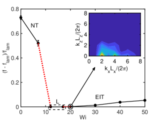
Figure 1: Scaled friction factor vs. $\mathrm{Wi}$ at $\mathrm{Re}=1500$. Abbreviations ‘NT’, ‘L’ and ‘EIT’ stand for Newtonian-like turbulence, laminar and elastoinertial turbulence, respectively. In most cases, the error bars are smaller than the symbols. Red dotted lines indicate the intervals of $\mathrm{Wi}$ in which the NT solution loses existence and the EIT solution comes into existence, respectively, as $\mathrm{Wi}$ increases. Inset shows the spatial spectrum of the wall normal velocity at $y=0$ for $\mathrm{Wi}=20$. Here, $x$- and $z$-wavenumbers $k_{x}$ and $k_{z}$ are reported in scaled form, as $k_{x}L_{x}/2\pi$ and $k_{z}L_{z}/2\pi$ . For inset, low is blue, high is yellow.

Fig. 1 illustrates 3D DNS results for scaled friction factor $(f-f_{\mathrm{lam}})/f_{\mathrm{lam}}$ vs. Weissenberg number $\mathrm{Wi}$ at $\mathrm{Re}=1500$. At low but increasing $\mathrm{Wi}$, the flow is turbulent, with $f$ decreasing, indicating that the drag is reduced from the Newtonian value. In this regime, which we denote NT, the turbulence displays a streamwise vortex structure typical of Newtonian turbulence. With a further increase in $\mathrm{Wi}$, however, $f-f_{\mathrm{lam}}$ drops to zero – the flow relaminarizes, as the NT regime loses existence. (At this $\mathrm{Re}$ and all $\mathrm{Wi}$ considered here, the laminar state is linearly stable.) At still higher $\mathrm{Wi}$, the flow, if seeded with a sufficiently energetic initial condition, becomes turbulent again, with a very low value of $f-f_{\mathrm{lam}}$ (consistent with experimental observations of Choueiri et al. (2018) in pipe flow) and a very different structure: i.e. a new kind of turbulence comes into existence. In this regime the flow structure corresponds to EIT as described by Samanta et al. (2013); Sid et al. (2018); we further analyze this structure below. In short, as $\mathrm{Wi}$ increases from zero, the self-sustaining mechanism of Newtonian turbulence is weakened by viscoelasticity, resulting in loss of existence of the NT state. As $\mathrm{Wi}$ increases further, a new nonlinear self-sustaining (i.e. bypass transition) mechanism comes into play, resulting in EIT.

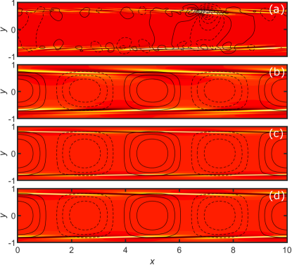
Figure 2: (a) Snapshot of $v^{\prime}$ (line contours) and $\alpha_{xx}^{\prime}$ (filled contours) from 3D nonlinear DNS at $\mathrm{Re}=1500$, $\mathrm{Wi}=20$, where ^′ denotes fluctuations. (b) Phase-matched average $(k_{x}L_{x}/2\pi,k_{z}L_{z}/2\pi)=(2,0)$ structures from 3D DNS. (c) Structure of the TS mode at $\mathrm{Re}=1500,\mathrm{Wi}=20$, and the same wavenumbers as in (b). (d) Structure of the most strongly amplified resolvent mode at $\mathrm{Re}=1500,\mathrm{Wi}=20$, the same wavenumbers as in (b), and $c=0.37$. In all plots, contour levels are symmetric about zero. For $v^{\prime}$ dashed - negative, solid - positive. For $\alpha_{xx}^{\prime}$ black - negative, red - zero and yellow - positive.

We now focus on the flow structure in the EIT regime. The inset in Fig. 1 shows a spatial spectrum of the wall normal velocity at $y=0$ (the channel centerplane), i.e., $|v(k_{x},0,k_{z})|$. The centerplane is chosen because it yields the cleanest spectra. In the EIT regime, there is very strong spectral content when $k_{z}=0$, indicating the importance of 2D mechanisms in the dynamics. Indeed, Sid et al. (2018) reports that EIT can arise in 2D simulations. Figure 2a shows a slice at $z=2.5$ of the fluctuating wall normal velocity, $v^{\prime}$, and fluctuating $xx$-component of the polymer conformation tensor, $\alpha^{\prime}_{xx}$. Observe that $\alpha^{\prime}_{xx}$ is strongly localized near $y=\pm 0.7-0.8$. While tilted sheets of polymer stretch fluctuations have already been noted as characteristic of EIT Samanta et al. (2013), the strong localization has not been previously observed, perhaps because prior results have been at higher $\mathrm{Re}$ and $\mathrm{Wi}$, i.e. further from the point at which EIT comes into existence. Fig. 2b shows the dominant $(k_{x}L_{x}/2\pi,k_{z}L_{z}/2\pi)=(2,0)$ component of the $\mathrm{Wi}=20$ results, phase-matched and averaged over many snapshots. Results for higher $k_{x}$ are very similar, exhibiting strong localization of stress fluctuations in the same narrow bands, as well as velocity fluctuations that span the channel height.

Linear analyses:

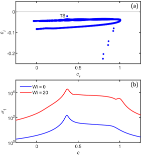
Figure 3: Eigenvalue spectrum for $(k_{x}L_{x}/2\pi,k_{z}L_{z}/2\pi)=(2,0)$ with $\mathrm{Wi}=20$ and $\mathrm{Re}=1500$. The eigenvalue labeled ‘TS’ corresponds to the TS mode. (b) Leading singular value of the resolvent operator for $\mathrm{Wi}=0$ and $\mathrm{Wi}=20$, plotted on a logarithmic scale.

To shed light on the origin of the highly localized large stress fluctuations, we now consider the evolution of infinitesimal perturbations to the laminar state with given wavenumbers $k_{x},k_{z}$. Two approaches are used. The first is classical linear stability analysis, in which solutions of the form $\phi(y)\exp\left[i\!\left(k_{x}x+k_{z}z-k_{x}ct\right)\right]$ are sought, resulting in an eigenvalue problem for the complex wavespeed $c$. If any $c_{i}>0$, then the laminar state is linearly unstable – infinitesimal perturbations will grow exponentially. If all $c_{i}<0$, the flow is linearly stable. The second approach is to determine the linear response of the laminar flow to external forcing with given real frequency $\omega$ using the resolvent operator (frequency-space transfer function) of the linearized equations Schmid (2007); McKeon and Sharma (2010). In both analyses, the concept of critical layers, i.e., wall-normal positions where the fluid velocity equals the wavespeed of an eigenmode or resolvent mode, is important. While some recent studies suggest the importance of critical-layer mechanisms in viscoelastic shear flows Page and Zaki (2015); Lee and Zaki (2017); Haward et al. (2018); Hameduddin et al. (2019), they do not make as direct a connection to EIT as we illustrate here.

Figure 3a shows the result of linear stability analysis (the eigenvalues $c$) for $\mathrm{Wi}=20$, $k_{x}L_{x}/2\pi=2$, $k_{z}=0$, the wavenumber corresponding to the dominant structures observed in the nonlinear simulations. All eigenvalues have $c_{i}<0$ – the laminar flow is linearly stable.

Of note is the mode labeled ‘TS’, the viscoelastic continuation of the classical Tollmien-Schlichting mode Drazin and Reid (2004). Viscoelasticity has only a weak effect on the TS eigenvalue, which changes from $c=0.362-0.019i$ to $c=0.368-0.022i$ between $\mathrm{Wi}=0$ and $\mathrm{Wi}=20$ Zhang et al. (2013). Despite the small change in $c$, the conformation tensor disturbance depends very strongly on $\mathrm{Wi}$; the peak value of $\alpha^{\prime}_{xx}$ grows from zero at $\mathrm{Wi}=0$ to $\sim\!10^{5}$ times the peak value of $u^{\prime}$ at $\mathrm{Wi}=20$.

The structure of this eigenmode is shown for $\mathrm{Wi}=20$ in Fig. 2c. In the Newtonian case, the disturbance velocity field is a train of spanwise-oriented vortices that span the entire channel; this structure is only weakly modified even at high $\mathrm{Wi}$. The polymer stress disturbance behaves very differently: at $\mathrm{Wi}=20$ it consists of highly inclined sheets that are extremely localized around the critical layers $y=\pm 0.79$ for the TS wavespeed of $c_{r}\approx 0.37$. Comparison with Figs. 2a and 2b shows a strong similarity between the eigenmode and the tilted sheetlike structures that are the hallmark of EIT, with the resemblance between the TS mode and the $(k_{x}L_{x}/2\pi,k_{z}L_{z}/2\pi)=(2,0)$ structure from the DNS in Fig. 2b being particularly striking. Specifically, note that for the TS mode, Fig. 2c, $v^{\prime}$ and $\alpha_{xx}^{\prime}$ are even and odd, respectively, with respect to $y=0$, while in Fig. 2b and the corresponding results at higher wavenumbers, these symmetries hold to a good approximation.

Despite the fact that the TS mode ultimately decays, the non-normal character of the linearized Navier-Stokes operator can lead to significant disturbance growth at short times or significant amplification of harmonic-in-time disturbances Schmid (2007). Thus it is therefore possible for small disturbances to be sufficiently amplified that nonlinear effects become significant. We now quantify this amplification by computing the largest singular value $\sigma_{1}$ of the resolvent operator. Figure 3b shows results for $\mathrm{Wi}=0$ and $\mathrm{Wi}=20$ in the same range of (real) wavespeeds $c=\omega/k_{x}$ depicted in Figure 3a. The amplification increases dramatically with $\mathrm{Wi}$, with the values at $\mathrm{Wi}=20$ being $\sim\!10^{2}$ times those for $\mathrm{Wi}=0$; this is consistent with the drastic increase in the conformation tensor disturbance amplitude already discussed for the TS mode. In both cases, the maximum amplification occurs for $c\approx 0.37$, which coincides with the wavespeed for the TS mode, indicating that the most-amplified disturbance is closely linked to the TS wave. Figure 2d shows the leading resolvent mode, which is indeed almost identical to the TS eigenmode in Figure 2c. This result provides additional strong evidence that the structures observed in EIT are closely related to those in viscoelasticity-modified TS waves.

It was recently shown that viscoelastic pipe flow of an Oldroyd-B fluid ($b\rightarrow\infty$) can be linearly unstable to center-localized modes with wavespeed $c_{r}\approx 1$ Garg et al. (2018). We estimate that for the present parameter values, this mode only becomes relevant for very high $\mathrm{Wi}$. Furthermore, center-localized structures are not observed in the simulations of EIT, so we do not consider them relevant here.

Self-sustained viscoelastic Tollmien-Schlichting waves:

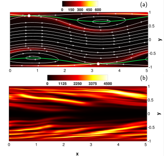
Figure 4: (a) Structure of nonlinear self-sustaining TS wave at $\mathrm{Re}=3000,\mathrm{Wi}=3$. White streamlines, shown in a reference frame moving with the wavespeed $c=0.39$, are superimposed on color contours of $\alpha_{xx}$. Green lines indicate the instantaneous critical layer positions, and white dots indicate the locations of hyperbolic stagnation points. (b) Snapshot of $\alpha_{xx}$ contours from 2D EIT at $\mathrm{Re}=3000$, $\mathrm{Wi}=15$.

Here we elaborate on the potential connection between TS-like structure and EIT, presenting results for nonlinear viscoelastic TS waves, i.e. self-sustained traveling wave solutions of the full nonlinear governing equations, illustrating the role of the critical-layer kinematics in generating localized sheetlike regions of high polymer stretching like those observed in EIT.

The strong peak in the EIT spectrum seen in Figure 1 corresponds to a wavelength of $5$, so here we report computations of nonlinear TS wave in a 2D domain with this length. The upper branch of this solution family is linearly stable in 2D at $\mathrm{Re}=3000$ Jiménez (1990); Mellibovsky and Meseguer (2015); Herbert (1979) and easily captured with DNS using the linear TS mode as the initial condition. In Newtonian flow, the solution family exists at this wavelength down to $\mathrm{Re}\approx 2800$. We continue the Newtonian solution at $\mathrm{Re}=3000$ to the parameters of interest ($\beta=0.97$ and $b=6400$) at $\mathrm{Wi}=0.1$, then increase $\mathrm{Wi}$ to study the effect of viscoelasticity. Hameduddin et al. Hameduddin et al. (2019) have computed nonlinear viscoelastic TS waves in the regime $\mathrm{Re}>5772$ and noted the role the critical layer plays in polymer stretching at high $\mathrm{Wi}$, but have not reported the observations described below.

On increasing $\mathrm{Wi}$, the self-sustained nonlinear viscoelastic TS wave at $\mathrm{Re}=3000$ develops sheets of high polymer stretch resembling near wall structures seen at EIT. Figure 4 illustrates this point with a plot of $\alpha_{xx}$ at $\mathrm{Wi}=3$. The source of this stretching is closely tied to the critical-layer structure of the TS wave velocity field. Critical layers have long been-known to exhibit a so-called Kelvin cat’s-eye streamline structure Drazin and Reid (2004) – indeed, the velocity fields for the flows shown in Figures 2c and 2d display this feature. With regard to viscoelasticity, the cat’s-eye structure is important because it contains hyperbolic stagnation points: polymers are strongly stretched as they approach such points and leave along their unstable manifolds. This phenomenon is clearly seen in Figure 4a; shown in white are streamlines in the reference frame traveling with the speed of the wave $c=0.39$, and in green is the instantaneous critical-layer position, i.e. where $v_{x}=c$. A hyperbolic stagnation point (white dot) exists at $x=3.22,y=-0.87$. The high polymer stretching follows the streamlines along the unstable directions associated with this point, giving rise to an arched sheetlike structure. By symmetry, identical structures exist in the top half of the channel. For comparison, Figure 4b shows $\alpha_{xx}$ for 2D EIT at $\mathrm{Re}=3000,\mathrm{Wi}=15$. This takes the form of tilted sheets of high polymer stretch starting out at locations close to the walls, and in fact reasonably close to the positions $y=\pm 0.87$ of the stagnation points in the nonlinear TS wave at $\mathrm{Wi}=3$. This similarity in structures suggests a role for TS wave-like critical-layer mechanisms at EIT. Indeed, these results suggest that the nonlinear TS wave solution branch may be directly connected in parameter space to EIT. We do not find this to be the case at $\mathrm{Re}=3000$; the TS branch loses existence above $\mathrm{Wi}\approx 4$ and the EIT branch loses existence below $\mathrm{Wi}\approx 13$. Nevertheless, when using the EIT result at $\mathrm{Wi}=13$ as the initial condition for a simulation at $\mathrm{Wi}=12$, EIT persists transiently for hundreds of time units and the last remaining structure observed as the flow decays to laminar closely resembles Figs. 2b-d.

Conclusion

Elastoinertial turbulence at low $\mathrm{Re}$ has strongly localized stress fluctuations, suggesting the importance of critical-layer mechanisms in its origin. These fluctuations strongly resemble the most slowly decaying structures from linear stability analysis, as well as the most strongly amplified disturbances as determined by resolvent analysis of the linearized equations. Furthermore, the Kelvin cat’s eye kinematics found in the critical-layer region of self-sustained nonlinear TS waves generate sheetlike structures in the stress field that resemble those observed in EIT. Taken together, these results suggest that, at least in the parameter range considered here, the bypass transition leading to EIT is mediated by nonlinear amplification and self-sustenance of perturbations that generate TS-wave-like flow structures.

This work was supported by (UW) NSF through grant CBET-1510291, AFOSR through grants FA9550-15-1-0062 and FA9550-18-1-0174, and ONR through grants N00014-18-1-2865 and (Caltech) N00014-17-1-3022.

A.S. and R.M.M. contributed equally to this work.

References

- Virk et al. (1970) P. S. Virk, H. S. Mickley, and K. A. Smith, J. Appl. Mech. 37, 488 (1970).
- Forame et al. (1972) P. C. Forame, R. J. Hansen, and R. C. Little, AIChE Journal 18, 213 (1972).
- Hoyt (1977) J. W. Hoyt, Nature 270, 508 (1977).
- Choueiri et al. (2018) G. H. Choueiri, J. M. Lopez, and B. Hof, Phys. Rev. Lett. 120, 124501 (2018).
- Chandra et al. (2018) B. Chandra, V. Shankar, and D. Das, J. Fluid Mech. 844, 1052 (2018).
- Samanta et al. (2013) D. Samanta, Y. Dubief, M. Holzner, C. Schäfer, A. N. Morozov, C. Wagner, and B. Hof, Proc. Nat. Acad. Sci. 110, 10557 (2013).
- Dubief et al. (2013) Y. Dubief, V. E. Terrapon, and J. Soria, Phys. Fluids 25, 110817 (2013).
- Sid et al. (2018) S. Sid, V. E. Terrapon, and Y. Dubief, Phys. Rev. Fluids 3, 011301 (2018).
- Kurganov and Tadmor (2000) A. Kurganov and E. Tadmor, J. Comput. Phys. 160, 241 (2000).
- Vaithianathan et al. (2006) T. Vaithianathan, A. Robert, J. G. Brasseur, and L. R. Collins, J. Non-Newtonian Fluid Mech. 140, 3 (2006).
- Dallas et al. (2010) V. Dallas, J. Vassilicos, and G. Hewitt, Phys. Rev. E 82, 066303 (2010).
- Hameduddin et al. (2019) I. Hameduddin, D. F. Gayme, and T. A. Zaki, J. Fluid Mech. 858, 377 (2019).
- Schmid (2007) P. J. Schmid, Annu. Rev. Fluid Mech. 39, 129 (2007).
- McKeon and Sharma (2010) B. J. McKeon and A. S. Sharma, J. Fluid Mech. 658, 336 (2010).
- Page and Zaki (2015) J. Page and T. A. Zaki, J. Fluid Mech. 777, 327 (2015).
- Lee and Zaki (2017) S. J. Lee and T. A. Zaki, J. Fluid Mech. 820, 232 (2017).
- Haward et al. (2018) S. J. Haward, J. Page, T. A. Zaki, and A. Q. Shen, Phys. Rev. Fluids 3, 091302 (2018).
- Drazin and Reid (2004) P. G. Drazin and W. H. Reid, Hydrodynamic Stability, 2nd ed., Cambridge Mathematical Libraries (Cambridge University Press, 2004).
- Zhang et al. (2013) M. Zhang, I. Lashgari, T. A. Zaki, and L. Brandt, J. Fluid Mech. 737, 249 (2013).
- Garg et al. (2018) P. Garg, I. Chaudhary, M. Khalid, V. Shankar, and G. Subramanian, Phys. Rev. Lett. 121, 024502 (2018).
- Jiménez (1990) J. Jiménez, J. Fluid Mech. 218, 265 (1990).
- Mellibovsky and Meseguer (2015) F. Mellibovsky and A. Meseguer, J. Fluid Mech. 779, R1 (2015).
- Herbert (1979) T. Herbert, in Proceedings of the Fifth International Conference on Numerical Methods in Fluid Dynamics June 28–July 2, 1976 Twente University, Enschede (Springer, 1979) pp. 235–240.