Supplementary materials of ”Linear statistics and pushed Coulomb gas at the edge of $\beta$-random matrices: four paths to large deviations”

Abstract

We give the details of the derivations described in the Letter. We explain all the connections between the four methods to study the large deviations. We give all details of the applications of these methods to various systems.

1 Mathematical preliminaries

We display here some useful formula for the calculations presented in this Letter.

1.1 Square root of the Heaviside function

We recall the notation from the Letter $\frac{1}{\sqrt{(\lambda)_{+}}}=\frac{\theta(\lambda)}{\sqrt{\lambda}}$ and introduce the following integral

$$\frac{1}{\pi}\int_{-\infty}^{+\infty}\frac{\rmd V}{\sqrt{(A-V)_{+}(V-A^{\prime})_{+}}}=\theta(A-A^{\prime})$$ (1)

where $A,A^{\prime}$ are real constants and $\theta$ is the Heaviside function. We further write this relation in a reduced convolution form

$$\frac{1}{\pi}\frac{1}{\sqrt{(\lambda)_{+}}}*\frac{1}{\sqrt{(\lambda)_{+}}}=\theta$$ (2)

From the convolution point of view, the function $1/\sqrt{(\lambda)_{+}}$ thus acts as a square root of the Heaviside function. Integrating this relation leads to the useful identity

$$\frac{2}{\pi}\int_{-\infty}^{+\infty}\rmd V\frac{\sqrt{(V-A^{\prime})_{+}}}{\sqrt{(A-V)_{+}}}=(A-A^{\prime})_{+}$$ (3)

1.2 Hilbert transform

Let us recall the definition of the Hilbert transform of a function $f$, as the convolution integral

$$H(f)(b)=\frac{1}{\pi}\mathchoice{{\vbox{\hbox{$\textstyle-$}}\kern-4.86108pt}}{{\vbox{\hbox{$\scriptstyle-$}}\kern-3.25pt}}{{\vbox{\hbox{$\scriptscriptstyle-$}}\kern-2.29166pt}}{{\vbox{\hbox{$\scriptscriptstyle-$}}\kern-1.875pt}}\!\int_{-\infty}^{+\infty}\rmd b^{\prime}\,\frac{f(b^{\prime})}{b-b^{\prime}}$$ (4)

where $\mathchoice{{\vbox{\hbox{$\textstyle-$}}\kern-4.86108pt}}{{\vbox{\hbox{$\scriptstyle-$}}\kern-3.25pt}}{{\vbox{\hbox{$\scriptscriptstyle-$}}\kern-2.29166pt}}{{\vbox{\hbox{$\scriptscriptstyle-$}}\kern-1.875pt}}\!\int$ is the Cauchy principal value. It is an anti-involution as $H(H(f))=-f$. The alternative expression

$$H(f)=\frac{1}{\pi}(\log\mathinner{\!\left\lvert.\right\rvert}*f)^{\prime}$$ (5)

will be useful below. From a simple residue calculation, one obtains the Hilbert transform of $1/\sqrt{(\lambda-A)_{+}}$ for a constant $A$ as

$$\frac{1}{\pi}\mathchoice{{\vbox{\hbox{$\textstyle-$}}\kern-4.86108pt}}{{\vbox{\hbox{$\scriptstyle-$}}\kern-3.25pt}}{{\vbox{\hbox{$\scriptscriptstyle-$}}\kern-2.29166pt}}{{\vbox{\hbox{$\scriptscriptstyle-$}}\kern-1.875pt}}\!\int_{-\infty}^{+\infty}\rmd\lambda^{\prime}\frac{1}{\lambda-\lambda^{\prime}}\frac{1}{\sqrt{(\lambda^{\prime}-A)_{+}}}=-\frac{1}{\sqrt{(A-\lambda)_{+}}}$$ (6)

From the anti-involution property of the Hilbert transform, one further has

$$\frac{1}{\pi}\mathchoice{{\vbox{\hbox{$\textstyle-$}}\kern-4.86108pt}}{{\vbox{\hbox{$\scriptstyle-$}}\kern-3.25pt}}{{\vbox{\hbox{$\scriptscriptstyle-$}}\kern-2.29166pt}}{{\vbox{\hbox{$\scriptscriptstyle-$}}\kern-1.875pt}}\!\int_{-\infty}^{+\infty}\rmd\lambda^{\prime}\frac{1}{\lambda-\lambda^{\prime}}\frac{1}{\sqrt{(A-\lambda^{\prime})_{+}}}=\frac{1}{\sqrt{(\lambda-A)_{+}}}$$ (7)

2 Details for the Section ”SAO/WKB method”

2.1 Semi-classical density of states

In the Letter we use the standard WKB argument [1, 2] to obtain the semi-classical density of states associated to a Schrödinger Hamiltonian describing a quantum particle of mass $m$ in a potential $W(x)$ in one dimension

$${\cal H}(p,x)=\frac{p^{2}}{2m}+W(x)\quad,\quad p=\frac{\hbar}{i}\partial_{x}$$ (8)

One considers classical periodic trajectories between two consecutive turning points $x_{\pm}$ where the classical momentum $p(x)=\sqrt{2m(E-W(x))}$ vanishes. In the limit of small $\hbar$, or for high energy levels, the quantification condition for the $n$-th level becomes well approximated by $\int_{x_{-}}^{x_{+}}\rmd x\,p(x)=\pi n\hbar$. Hence the integrated density of states, i.e. the number of levels below the energy $E$

$$N(E)=\frac{1}{\hbar\pi}\int\rmd x\,\sqrt{2m(E-W(x))}$$ (9)

Taking from Eq. (8) of the Letter, ${\cal H}={\cal H}^{\prime}_{SAO}$, which corresponds to $W(x)=x+v(x)$, $m=1/2$, $E=b$ and $\hbar=1/t$, we can apply for large $t$ this WKB estimate leading to the formula (9) in the Letter. There we consider that there is an infinite barrier at $x=0$, hence $x_{-}=0$ and $x_{+}$ denotes the first turning point.

The highly surprising, and quite non-trivial point is that this can be a useful approximation despite the fact that $v(x)$ is not at all smooth. One way to understand it is to remember that in effect the approximation is used for describing the optimal $v(x)$ (or near optimal one) which is way smoother, as we find.

An equivalent way to justify the starting point for the density is to use the Ricatti equation. Writing first the Schrödinger equation ${\cal H}^{\prime}_{SAO}\psi=b\psi$ and introducing $g(x)=\psi^{\prime}(x)/\psi(x)$ it is well known [3, 5, 4, 6] that the number of eigenvalues below level $b$, $N(b)=N(b_{i}<b)$, of ${\cal H}^{\prime}_{SAO}$ equals the total number of explosions of the Ricatti equation satisfied by $g$

$$g^{\prime}(x)=t^{2}(x-b+v(x))-g(x)^{2}\quad,\quad g(0)=+\infty$$ (10)

It turns out that in the limit of a large parameter $t$ the blow ups are very densely spaced in $x$, hence in each blow up interval we can solve this equation assuming that ${\sf b}={\sf b}(x)\mathrel{\mathop{\mathchar 58\relax}}=b-x-v(x)>0$ is constant. The equation is then

$$g^{\prime}(x)=-t^{2}{\sf b}-g^{2}$$ (11)

and its solution is $g(x)=-t\sqrt{{\sf b}}\tan(t\sqrt{{\sf b}}x+C)$: if $x_{i}$ denote the $i$-th blow up time the separation in $x$ between two consecutive blow up

$$x_{i+1}-x_{i}=\frac{\pi}{t\sqrt{{\sf b}(x_{i})}}\ll 1$$ (12)

is indeed small in the semi-classical limit, i.e. for large $t$ (note that for ${\sf b}<0$ there is no blow up). Taking a continuum limit we can write $\frac{\rmd x}{\rmd i}=\frac{\pi}{t\sqrt{b(x)}}$ leading to

$$N(\lambda_{i}<b)=\frac{1}{t}\int_{-\infty}^{b}\rmd b^{\prime}\,\hat{\rho}(b^{\prime})\simeq\frac{1}{\pi}\int_{0}^{+\infty}\rmd x\,\sqrt{(b-x-v(x))_{+}}$$ (13)

which leads to Eq. (9) in the Letter. This argument was sketched to us by L.C. Tsai and later made rigorous by him in the case of the application to $\phi=\phi_{\rm KPZ}$ in Ref. [6].

2.2 Simplification of $\Sigma_{\phi}(u)$ at the saddle point SP1

Let us derive now the expression of $\Sigma_{\phi}(u)$ taken at the saddle point expression Eq. (12) in the Letter. We have

$$\Sigma_{\phi}(u)=\int_{-\infty}^{+\infty}\mathrm{d}b\,\rho_{*}(b)\phi(u-b)+\frac{\beta}{8}\int_{0}^{+\infty}\mathrm{d}x\,v_{*}(x)^{2}$$ (14)

where $v_{*}(x)$ is the solution of the saddle point SP1 and $\rho_{*}(b)$ is the optimal density

$$\frac{\beta}{4}v_{*}(x)=\frac{1}{2\pi}\int_{0}^{+\infty}\frac{\mathrm{d}b}{\sqrt{b}}\phi^{\prime}(u-b-x-v_{*}(x))\quad,\quad\rho_{*}(b)=\frac{1}{2\pi}\int_{0}^{+\infty}\rmd x\,\frac{1}{\sqrt{(b-x-v_{*}(x))_{+}}}$$ (15)

Let us transform the first term as

$$\begin{split}\int_{-\infty}^{+\infty}\mathrm{d}b\,\rho_{*}(b)\phi(u-b)&=\frac{1}{2\pi}\int_{-\infty}^{+\infty}\mathrm{d}b\int_{0}^{+\infty}\rmd x\,\frac{\phi(u-b)}{\sqrt{(b-x-v_{*}(x))_{+}}}\\ &=\frac{1}{2\pi}\int_{0}^{+\infty}\mathrm{d}b\int_{0}^{+\infty}\rmd x\,\frac{1}{\sqrt{b}}\phi(u-b-x-v_{*}(x))\\ &=\frac{1}{2\pi}\int_{0}^{+\infty}\mathrm{d}b\int_{0}^{+\infty}\rmd x\,x(1+v_{*}^{\prime}(x))\frac{1}{\sqrt{b}}\phi^{\prime}(u-b-x-v_{*}(x))\\ &=\frac{\beta}{4}\int_{0}^{+\infty}\rmd x\,x\big{(}1+v_{*}^{\prime}(x)\big{)}v_{*}(x)\\ &=\frac{\beta}{4}\int_{0}^{+\infty}\rmd x\,\big{(}xv_{*}(x)-\frac{v_{*}(x)^{2}}{2}\big{)}\end{split}$$ (16)

The transformation from the first line to the second is a shift of $b$ by $x+v_{*}(x)$. From the second to the third line we proceeded to an integration by part with respect to $x$. From the third to the fourth, we used the saddle point SP1 and finally from the fourth to the fifth, we integrated by part the $v_{*}v_{*}^{\prime}$ term. We observe that the quadratic term $v_{*}^{2}$ cancels the one from the Brownian measure in $\Sigma_{\phi}(u)$ therefore leading to Eq. (12) from the Letter

$$\Sigma_{\phi}(u)=\frac{\beta}{4}\int_{0}^{+\infty}\rmd x\,xv_{*}(x)$$ (17)

2.3 Simplification of $\Sigma^{\prime}_{\phi}(u)$ at the saddle point SP1

The derivative of the free energy $\Sigma_{\phi}(u)$ at the saddle point is obtained by taking the explicit derivative with respect to $u$ of Eq. (14), leading to $\Sigma^{\prime}_{\phi}(u)=\int_{-\infty}^{+\infty}\mathrm{d}b\,\rho_{*}(b)\phi^{\prime}(u-b)$. Inserting the WKB parametrization for the density and using the saddle point equation SP1, we get

$$\begin{split}\int_{-\infty}^{+\infty}\mathrm{d}b\,\rho_{*}(b)\phi^{\prime}(u-b)&=\frac{1}{2\pi}\int_{-\infty}^{+\infty}\mathrm{d}b\int_{0}^{+\infty}\rmd x\,\frac{\phi^{\prime}(u-b)}{\sqrt{(b-x-v_{*}(x))_{+}}}\\ &=\frac{1}{2\pi}\int_{0}^{+\infty}\mathrm{d}b\int_{0}^{+\infty}\rmd x\,\frac{1}{\sqrt{b}}\phi^{\prime}(u-b-x-v_{*}(x))\\ &=\frac{\beta}{4}\int_{0}^{+\infty}\rmd x\,v_{*}(x)\\ &=\frac{1}{\pi}\int_{0}^{u}\rmd u^{\prime}\,w(u^{\prime})\end{split}$$ (18)

which provides another way to show that $\Sigma_{\phi}^{\prime\prime}(u)=\frac{1}{\pi}w(u)$ as stated in the Letter. Note that Eq. (18) can directly be obtained from Eq. (17) using the correspondence $v_{*}(x)=\frac{4}{\beta\pi}w(u-x)$ implying that $\partial_{u}v_{*}=-\partial_{x}v_{*}$ at the saddle point.

3 Details for the Section ”cumulant method”

3.1 Cumulant expansion for $\Sigma_{\phi}(u)$

Although we will insert factors of $\beta/2$ in some formulae here, the derivation here is restricted to $\beta=2$. As discussed in the Letter, comparison with the other methods validates our proposed extension to arbitrary $\beta$. The expectation $Q_{t}(u)$ defined in the Letter in Eq. (5) over the Airy point process for $\beta=2$ can be expressed as a Fredholm determinant (see also Eq. (19) in the Letter)

$$Q_{t}(u)=\mathrm{Det}[I-\sigma_{t}K_{{\rm Ai}}]_{\,\mathbb{L}^{2}(\mathbb{R})}$$ (19)

where $I$ is the identity operator, $\sigma_{t}(a)=1-e^{-t\phi(u+t^{-2/3}a)}$ and $K_{{\rm Ai}}(a,a^{\prime})$ is the Airy kernel, i.e. $K_{\mathrm{Ai}}(a,a^{\prime})=\int_{0}^{\infty}\!\rmd r\;\mathrm{Ai}(r+a)\mathrm{Ai}(r+a^{\prime})$. Let us recall the results of Ref. [7] providing the expansion in cumulants of Fredholm determinants such as (19) with the choice of functions $\sigma_{t}(a)=1-\exp[g_{t}(\sigma e^{at^{1/3}})]$ for a class of functions $g_{t}$. The expansion in cumulants is defined by the following series

$$\log\mathrm{Det}\left[I-(1-\rme^{\alpha\hat{g}})K_{{\rm Ai}}\right]=\sum_{n=1}^{\infty}\frac{\alpha^{n}\kappa_{n}}{n!}$$ (20)

where we denote $\hat{g}(a)=g_{t}(\sigma e^{t^{1/3}a})$, $Q_{t}(u)$ being obtained by setting the book-keeping parameter $\alpha$ to 1. The first two cumulants are given by $\kappa_{1}=\mathrm{Tr}(\hat{g}K_{{\rm Ai}})$ and $\kappa_{2}=\mathrm{Tr}(\hat{g}^{2}K_{{\rm Ai}})-\mathrm{Tr}(\hat{g}K_{{\rm Ai}}\hat{g}K_{{\rm Ai}})$, see [7, 8, 9] for more details. It was found in Ref. [7] that the cumulants can be written as

$$\kappa_{n}=t^{\frac{n}{2}-1}2^{n-1}(\sigma\partial_{\sigma})^{n-3}\mathfrak{L}_{1}(\sigma)^{n}+\dots$$ (21)

where

$$\mathfrak{L}_{1}(\sigma)=\frac{1}{\pi}(\sigma\partial_{\sigma})^{2}\int_{0}^{+\infty}\mathrm{d}x\sqrt{x}g_{t}(\sigma e^{-x})$$ (22)

As discussed in Ref. [7], under some conditions, the term displayed in Eq. (21) is dominant compared to the (complicated) remainder indicated by the $"\dots"$, this is case for large time if one chooses $\sigma=-e^{ut}$ and functions such that

$$\lim_{t\to+\infty}-\frac{g_{t}(-e^{t(u+b)})}{t}=\phi(u+b)$$ (23)

and $g_{t}(0)=0$, which is precisely what is needed for the results to apply to the class of functions $\sigma_{t}(a)=1-e^{-t\phi(u+t^{-2/3}a)}$. Note that $g(0)=0$ implies that $\phi(x)=0$ for $x\leq 0$. Inserting $\sigma=-e^{ut}$ into Eqs. (21) and (22) and taking the large time limit Eq. (23), the $n$-th cumulant reads (until now for $\beta=2$)

$$\kappa_{n}=t^{\frac{n}{2}-1}\frac{2^{n-1}}{\pi^{n}}(\frac{1}{t}\partial_{u})^{n-3}\left(-\frac{1}{t}(\partial_{u})^{2}\int_{0}^{+\infty}\mathrm{d}x\sqrt{x}\phi(u-\frac{x}{t})\right)^{n}$$ (24)

Regrouping the different factors, one observes that all leading terms of $\kappa_{n}$ are proportional to $t^{2}$ and we can then write the summation over the cumulant index $n$, and now insert appropriate factors of $\beta/2$, leading to

$$\log Q_{t}(u)=\sum_{n\geq 1}\frac{\kappa_{n}}{n!}=-t^{2}\Sigma_{\phi}(u)\quad,\quad\Sigma_{\phi}(u)=-\frac{\beta}{4}\sum_{n\geq 1}\frac{1}{n!}(-\frac{4}{\beta\pi})^{n}\partial_{u}^{n-3}f(u)^{n}$$ (25)

where

$$f(u)=\int_{\mathbb{R}}\rmd b\,\sqrt{(b)_{+}}\phi^{\prime\prime}(u-b)$$ (26)

Upon integration by part, one obtains formulae (13) and (14) as given in the Letter. For $n=1,2$ we clarify the meaning of the anti-derivative in Eq. (25) as

$$\begin{split}\kappa_{1}=-\frac{t^{2}}{\pi}\int_{0}^{+\infty}\mathrm{d}b\sqrt{b}\,\phi(u-b)=-\frac{t^{2}}{\pi}\int_{0}^{u}\int_{0}^{u^{\prime}}\rmd u^{\prime}\rmd u^{\prime\prime}f(u^{\prime\prime})\quad,\quad\kappa_{2}=\frac{4t^{2}}{\beta\pi^{2}}\int_{0}^{u}\rmd u^{\prime}\,f(u^{\prime})^{2}\end{split}$$ (27)

3.2 Cumulants of ${\sf L}$

The generating function of the cumulants of ${\sf L}$ can be obtained at large $t$ as

$$\log\mathbb{E}_{\beta}[e^{-B{\sf L}}]=\sum_{n\geq 1}\frac{(-B)^{n}}{n!}\mathbb{E}_{\beta}[{\sf L}^{n}]^{c}\simeq-t^{2}\Sigma_{B\phi}(u)$$ (28)

i.e. it can be obtained by the multiplication of $\phi$ by an amplitude $B$. Inserting $\phi\to B\phi$ in (25) and identifying order by order we obtain

$$\mathbb{E}_{\beta}[{\sf L}^{n}]^{c}=(-1)^{n}\kappa_{n}\simeq\frac{\beta}{4}t^{2}(\frac{4}{\beta\pi})^{n}\partial_{u}^{n-3}f(u)^{n}$$ (29)

where $\kappa_{1}$ and $\kappa_{2}$ are given explicitly in (27), the formula being quite explicit for $n\geq 3$. Note that in the Letter we use $\tilde{\kappa}_{n}(u)=\kappa_{n}/t^{2}$.

3.3 Resummation of $\Sigma_{\phi}(u)$

It is possible and convenient to perform the summation of the series representation of $\Sigma_{\phi}$ by writing its third derivative as

$$\Sigma_{\phi}^{\prime\prime\prime}(u)=-\frac{\beta}{4}\sum_{n\geq 1}\frac{1}{n!}(-\frac{4}{\beta\pi})^{n}(\partial_{u})^{n}f(u)^{n}$$ (30)

We have used a Mellin-Barnes summation method presented in the Appendix, and displayed in Eq. (301) with $a=-\frac{4}{\beta\pi}$ and $\Sigma_{\phi}^{\prime\prime\prime}(u)=-\frac{\beta}{4}\mathcal{S}(u)$. The summation is mapped to the problem of solving the following equation for $w=w(u)$

$$f(u-\frac{4}{\beta\pi}w)=w$$ (31)

We consider for now functions $f$ which are positive, increasing with $f(b)=0$ for $b\leq 0$. There is then a unique solution of Eq. (31) which can be written

$$u\mathrel{\mathop{\mathchar 58\relax}}=u(w)=f^{-1}(w)+\frac{4}{\beta\pi}w,\quad\forall w>0,\quad\text{and}\;u(0)=0$$ (32)

It is convenient to extend $w$ and $u$ to negative values setting $u(w\leq 0)=0$ and $w(u\leq 0)=0$. Given the uniqueness, from Eq. (301) and (309), $\Sigma_{\phi}^{\prime\prime\prime}$ is given by

$$\Sigma_{\phi}^{\prime\prime\prime}(u)=-\frac{\beta}{4}\left(\frac{1}{1+\frac{4}{\beta\pi}f^{\prime}(u-\frac{4}{\beta\pi}w(u))}-1\right)=\frac{1}{\pi}w^{\prime}(u)$$ (33)

We then perform the integrations, noting that for $u\to-\infty$ the Coulomb gas is not affected by the wall and $\Sigma_{\phi}(u)$ and its derivatives should vanish. For $\phi$ in $\Omega_{0}$, $f$ and $w$ vanish for $u\leq 0$, so we can even use that $\Sigma(0)=\Sigma^{\prime}(0)=\Sigma^{\prime\prime}(0)=0$. The first integration gives

$$\Sigma_{\phi}^{\prime\prime}(u)=\frac{1}{\pi}\int_{-\infty}^{u}\rmd u^{\prime}\,w^{\prime}(u^{\prime})=\frac{1}{\pi}w(u)$$ (34)

The second integration gives

$$\Sigma_{\phi}^{\prime}(u)=\frac{1}{\pi}\int_{-\infty}^{u}\rmd u^{\prime}\,w(u^{\prime})=\frac{1}{\pi}\int_{0}^{u}\rmd u^{\prime}w(u^{\prime})=\frac{1}{\pi}\int_{0}^{w(u)}\rmd w^{\prime}[u-u(w^{\prime})]$$ (35)

The third integration gives

$$\Sigma_{\phi}(u)=\frac{1}{2\pi}\int_{0}^{w(u)}\mathrm{d}w^{\prime}\left[u-u(w^{\prime})\right]^{2}=\frac{1}{\pi}\int_{0}^{u}\mathrm{d}u^{\prime}\,w(u^{\prime})\left[u-u^{\prime}\right]$$ (36)

The forms as integrals in $w^{\prime}$ are quite useful in practice when $f^{-1}(w)$ has a simple form, as in the examples given below, since $u(w)$ is then explicit using (32) and the integral can often be calculated. The second form is given in the Letter in Eq. (16) and allows easy comparison with the other methods.

4 Ensembles of functions $\phi$ considered for the linear statistics

It is useful to recapitulate the ensembles of functions $\phi$ considered here. The condition that for all $u$ in $A$ there is a unique solution $w=w(u)$ to

$$w=f(u-\frac{4}{\beta\pi}w)$$ (37)

is equivalent to the condition that for all $u$ in $A$ there is a unique solution $z=z(u)$ to

$$u=z+\frac{4}{\beta\pi}f(z)$$ (38)

with the relation $z(u)=u-\frac{4}{\beta\pi}w(u)$. This condition is in turn equivalent to the condition that $z\to h(z)=z+\frac{4}{\beta\pi}f(z)$ is strictly monotonous and has no jump (is continuous) in $h^{-1}(A)$. We call $\Omega_{2}$ the set of functions $\phi$ such that their associated $f$ has this property (where monotonous means increasing) with $A=\mathbb{R}$.

$$\Omega_{2}=\{\phi\mid z\mapsto z+\frac{4}{\beta\pi}f(z)\;\;\text{is strictly increasing and continuous}\}$$

We call $\Omega_{0}$, a subset of $\Omega_{2}$ such that $f(z)$ itself is increasing, positive, continuous with $f(z\leq 0)=0$.

$$\Omega_{0}=\{\phi\mid z\mapsto f(z)\;\;\text{is increasing positive and continuous},\;\;f(z\leq 0)=0\}$$

It implies that $\phi$ is also increasing, positive, continuous with $\phi(z\leq 0)=0$, however not all such functions are in $\Omega_{0}$ (roughly, $\phi$ has to grow fast enough on the positive side - e.g. if $\phi^{\prime}$ has these properties then $\phi$ is in $\Omega_{0}$). Since $w(u)=f(z(u))$ we see that if $\phi$ is in $\Omega_{2}$ but not in $\Omega_{0}$ then $w(u)$ may be non monotonous in $u$, or negative.

Finally, we define $\Omega_{1}$ the set of functions $\phi$ such that $f(z)$ is increasing, positive, continuous, but we do not require $f(z\leq 0)=0$.

$$\Omega_{1}=\{\phi\mid z\mapsto f(z)\;\;\text{is increasing positive and continuous}\}$$

Note that here we further require that $\lim_{b\to-\infty}(-b)^{3/2}\phi(b)=0$ to guarantee a finiteness of the excess energy (see Section on the inverse monomial walls).
We have the ordering relation $\Omega_{0}\subset\Omega_{1}\subset\Omega_{2}$. Most of the Letter focuses on the set $\Omega_{0}$, the monomial walls and an extension to $\Omega_{1}$, the exponential wall and the inverse monomial, will be presented.

For $\phi$ in $\Omega_{1}$ all formula presented in the Letter hold with the slight modification that $w(u)$ does not vanish for $u<0$ (but remains positive and vanishes at $u=-\infty$) hence all integrations over $u$ must start from $u=-\infty$ (while those over $w$ still start at 0). The saddle point $v_{*}(x)$ now is non zero for $x>u$ but keeps the same properties (positivity and $x+v(x)$ increasing) and vanishes at $x=+\infty$. The relations (17) and (26) in the Letter between $v_{*}$,$w$,$g$ remain true, i.e.

$$\begin{split}&\forall u\in\mathbb{R},\;w(u)=\frac{\beta\pi}{2}g(-u)\\ &\forall x\geq 0,\;v_{*}(x)=\frac{4}{\beta\pi}w(u-x)\end{split}$$ (39)

5 From WKB/SAO to the cumulant expansion

Let us now study the saddle point equation for the WKB/SAO method. Equation (11) in the Letter can be written as

$$\begin{split}\frac{\beta}{4}v_{*}(x)&=\frac{1}{2\pi}\int_{-\infty}^{+\infty}\frac{\rmd b}{\sqrt{(b)_{+}}}\phi^{\prime}(u-b-x-v_{*}(x))\\ &=\frac{1}{\pi}f(u-x-v_{*}(x))\end{split}$$ (40)

where we have used the definition of Eqs. (14) in the Letter and (26) in the Supp. Mat. of the function $f$. To make contact with the method of cumulants, we study a solution $v_{*}(x)$ which has the form

$$v_{*}(x)=\frac{4}{\beta\pi}w(u-x)\quad 0\leq x\leq u$$ (41)

with $v_{*}(x)=0$ for $x\geq u$. With this parametrization, the saddle point equation becomes

$$f(u-\frac{4}{\beta\pi}w(u))=w(u)$$ (42)

This is precisely the equation (31) encountered in the resummation of the series in the cumulant method. In addition, using this parametrization, the resulting equation for $\Sigma_{\phi}(u)$ within the WKB/SAO method Eq. (9) reads

$$\Sigma_{\phi}(u)=\frac{\beta}{4}\int_{0}^{+\infty}\rmd x\,x\,v_{*}(x)=\frac{1}{\pi}\int_{0}^{u}\rmd u^{\prime}w(u^{\prime})[u-u^{\prime}]$$ (43)

This identifies with the one Eq. (14) from the cumulant method. We now derive through the WKB/SAO method the series expansion previously obtained from the cumulant method. This is realized by the means of the Lagrange inversion formula. Let us recall that the Lagrange inversion formula states that for a sufficiently nice function $h$, the equation $z=x+yh(z)$ can be inverted as

$$z=x+\sum_{n\geq 1}\frac{y^{n}}{n!}(\partial_{x})^{n-1}h(x)^{n}$$ (44)

Identifying $x=u$, $z=u-\frac{4}{\beta\pi}w$, $y=-\frac{4}{\beta\pi}$, $h=f$ leads to a series representation for the solution $w(u)$ of Eq. (42)

$$-\frac{4}{\beta\pi}w(u)=\sum_{n\geq 1}\frac{1}{n!}(-\frac{4}{\beta\pi})^{n}\partial_{u}^{n-1}f(u)^{n}$$ (45)

From Eq. (43), we also have $\Sigma_{\phi}^{\prime\prime}(u)=\frac{1}{\pi}w(u)$ and hence we obtain

$$\Sigma_{\phi}^{\prime\prime}(u)=-\frac{\beta}{4}\sum_{n\geq 1}\frac{1}{n!}(-\frac{4}{\beta\pi})^{n}\partial_{u}^{n-1}f(u)^{n}$$ (46)

which coincides precisely with the second derivative of the series expansion obtained for the cumulant method (valid at $\beta=2$ and generalized there to arbitrary $\beta$).

6 Details for the Section ”Painlevé method”

6.1 Analysis of the non-local Painlevé equation

Let us recall here the analysis of Ref. [10] and present its generalization. To make it easier we stick to the notations of Ref. [10]. Starting from the equations (20-22) of the Letter we introduce as in Ref. [10] the scaled variables $r=t^{2/3}X$, $v=t^{2/3}V$ and make the ansatz $q_{t}(r,v)=t^{-1/6}\tilde{q}_{t}(X,V)$ and $\Psi_{t}(r)\simeq t^{2/3}g_{t}(X)$, with $g_{t}(X)>0$. The remarkable fact is that the function $g_{t}(X)$ becomes independent of $t$ at large $t$, and one denotes $g(X)=\lim_{t\to+\infty}g_{t}(X)$. Performing the rescaling, Eq. (21) in the Letter becomes

$$g(X)=\int_{-\infty}^{+\infty}\rmd V[\tilde{q}_{t}(X,V)]^{2}\phi^{\prime}(V)e^{-t\phi(V)}$$ (47)

It is precisely the condition that the r.h.s. does not depend on $t$ at large $t$ which leads to the two equations SP1 and SP2 (Eqs (23) and (24) in the Letter) and of the consistency of the ansatz, as we now discuss.

Performing the rescaling, the Eq. (22) of the Letter becomes

$$-t^{-2}\partial_{X}^{2}\tilde{q}_{t}(X,V)+(V+X+2g(X))\tilde{q}_{t}(X,V)=0$$ (48)

with the boundary condition $\tilde{q}_{t}(X,V)\to_{X\to+\infty}t^{1/6}{\rm Ai}(t(X+V))\simeq\frac{\exp(-\frac{2}{3}t(X+V)^{3/2})}{2\sqrt{\pi}(X+V)^{1/4}}$. It can be interpreted as the Schrödinger equation of a quantum particle of mass $m=1/2$ at energy $-V$ in the potential $X+2g(X)$, in the semi-classical limit since $\hbar=1/t$ is small. As in Ref [10] we consider cases such that $g(X)$ is a positive and monotonic decreasing function, and, as seen below, $g(X)$ vanishes for $X>0$. The potential $X+2g(X)$ is however an increasing function of $X$. Hence there is a unique classical turning point at $X=a$ with $V+a+2g(a)=0$. The classical momentum of the particle is $p(X,V)=\sqrt{-V-X-2g(X)}$, which is positive in the the classically allowed region $X<a$, and imaginary for $X>a$, the forbidden region. The standard WKB method then gives the following approximation of the wave function for large $t$

$$\begin{split}\tilde{q}_{t}(X,V)\simeq&\;\frac{C_{t}(V)}{|V+X+2g(X)|^{1/4}}\\ &\bigg{(}\cos\left[t\int_{-\infty}^{X}\rmd X^{\prime}\sqrt{(-V-X^{\prime}-2g(X^{\prime}))_{+}}-\frac{\pi}{4}\right]\theta(-V-X-2g(X))\\ &+\frac{1}{2}\exp\big{[}-t\int_{-\infty}^{X}\rmd X^{\prime}\sqrt{(V+X^{\prime}+2g(X^{\prime}))_{+}}\big{]}\;\theta(V+X+2g(X))\bigg{)}\end{split}$$

The boundary condition determines the amplitude $C_{t}(V)$ as

$$C_{t}(V)=\frac{1}{\sqrt{\pi}}\exp\left(t\int_{-\infty}^{+\infty}\rmd X^{\prime}\big{[}\sqrt{(V+X^{\prime}+2g(X^{\prime}))_{+}}-\sqrt{(V+X^{\prime})_{+}}\big{]}\right)$$ (49)

Inserting $\tilde{q}_{t}(X,V)$ into Eq. (47) we obtain a sum of two contributions

$$\begin{split}&g(X)=\int_{-\infty}^{+\infty}\rmd V\frac{C_{t}(V)^{2}\phi^{\prime}(V)e^{-t\phi(V)}}{|V+X+2g(X)|^{1/2}}\\ &\bigg{(}\frac{\theta(-V-X-2g(X))}{2}+\frac{\theta(V+X+2g(X))}{4}e^{-2t\int_{-\infty}^{X}\rmd X^{\prime}\sqrt{(V+X^{\prime}+2g(X^{\prime}))_{+}}}\bigg{)}\end{split}$$ (50)

The second term can be neglected at large $t$ compared to the first (see Ref. [10] for more discussion of the validity of the WKB approximations) leading to

$$\begin{split}g(X)=&\frac{1}{2\pi}\int_{-\infty}^{-X-2g(X)}\frac{\rmd V\phi^{\prime}(V)}{\sqrt{-V-X-2g(X)}}\\ &\exp\bigg{(}t\big{(}2\int_{-\infty}^{+\infty}\rmd X^{\prime}[\sqrt{(V+X^{\prime}+2g(X^{\prime}))_{+}}-\sqrt{(V+X^{\prime})_{+}}]-\phi(V)\big{)}\bigg{)}\end{split}$$ (51)

The condition of $t$ independence gives the two equations in the Letter, namely

$$g(X)=\frac{1}{2\pi}\int_{-\infty}^{-X-2g(X)}\frac{\rmd V\phi^{\prime}(V)}{\sqrt{-V-X-2g(X)}}$$ (52)

$$\phi(V)=2\int_{-\infty}^{+\infty}\rmd X^{\prime}\left[\sqrt{(V+X^{\prime}+2g(X^{\prime}))_{+}}-\sqrt{(V+X^{\prime})_{+}}\right]$$ (53)

If $\phi$ belongs to the class $\Omega_{0}$, $\phi^{\prime}(V)\geq 0$ and strictly vanishes for $V<0$ and one finds that indeed $g(X)\geq 0$ with $g(X)=0$ for $X>0$ as anticipated. Hence the upper bound of the integral in the second equation can be chosen to be $X^{\prime}=0$, recovering the Eq. (24) in the Letter. Finally, performing the rescaling in the Eq. (20) of the Letter leads to

$$\log Q_{t}(u)=-t^{2}\int_{-u}^{+\infty}\rmd X(u+X)g(X)$$ (54)

leading to the formula (25) in the Letter whenever $g(X>0)=0$.

The important property in the above derivation seems to be the uniqueness of the turning point, i.e. that $X\to X+g(X)$ is a strictly increasing function. Comparison with the other method (see below) suggests that it can be extended to cases where $g(X)$ does not vanish for $X>0$ but decays sufficiently fast so that the integral in (53) converges.

We note the amazingly close resemblance to the WKB analysis of the SAO operator. The connection is discussed in the Letter, and combining the equations (16) and (25) there we can identify

$$v_{*}(x)=2g(x-u)$$ (55)

where $v(x)$ is taken at the saddle point SP1. The property that $v(x>u)=0$ thus maps to the property that $g(X>0)=0$ (and holds for $\phi\in\Omega_{0}$). Note however that the function $g(X)$ also lives for any $X<u$, and so does $w(u)$ for any $u>0$, hence there is a natural extension of the function $v(x)$ of the SAO method.

Note that Eqs. (47), (48) and (54) are all exact for any $t$ if one replace $g(X)\to g_{t}(X)$ and equivalent to the system (20-22) in the Letter, being simply their scaled version. Hence there may be a more general connection, for arbitrary $t$. Each methods evaluate one line of the equality, for any $t$

$$\mathbb{E}_{v}\big{[}{\rm Det}[e^{-t\phi(u-{\cal H}^{\prime}_{SAO})}]\big{]} =\mathbb{E}_{v}[e^{-t{\rm Tr}\,\phi(u-{\cal H}^{\prime}_{SAO})}]$$ (57)

$$={\rm Det}[I-(1-e^{-t\phi(u+t^{-2/3}a)})K_{\rm Ai}]$$

6.2 Inversion formula between $f$ and $\phi$

We recall the definition of $f(u)$ as

$$f(u)=\frac{1}{2}\int_{-\infty}^{+\infty}\frac{\rmd b}{\sqrt{(b)_{+}}}\phi^{\prime}(u-b)=\frac{1}{2}\frac{1}{\sqrt{(b)_{+}}}*\phi^{\prime}$$ (58)

Note that $f(u)$ also vanishes for $u\leq 0$. We can convolute $f(u)$ and obtain

$$\frac{2}{\pi}\frac{1}{\sqrt{(b)_{+}}}*f=\frac{1}{\pi}\frac{1}{\sqrt{(b)_{+}}}*(\frac{1}{\sqrt{(b)_{+}}}*\phi^{\prime})=\theta*\phi^{\prime}=\phi$$ (59)

Hence the inversion formula

$$\phi(u)=\frac{2}{\pi}(\frac{1}{\sqrt{(b)_{+}}}*f)(u)=\frac{2}{\pi}\int_{-\infty}^{+\infty}\frac{\rmd b}{\sqrt{(b)_{+}}}f(u-b)$$ (60)

This inversion formula is now used to proof the miracle, i.e. Eq. (24) of the Letter.

6.3 Proof of the ”miracle” for arbitrary $\beta$ : SP1 $\Rightarrow$ SP2

For all $\beta$, let us define $\mathcal{I}$ by

$$\mathcal{I}=\beta\int_{0}^{+\infty}\rmd u^{\prime}\sqrt{(V-u^{\prime}+\frac{4}{\beta\pi}w(u^{\prime}))_{+}}-\frac{2\beta}{3}V^{3/2}$$ (61)

and we now prove that for all $V\geq 0$, $\mathcal{I}=\phi(V)$. Recalling that $w(u)=f(u-\frac{4}{\beta\pi}w(u))$, we perform the change of variable in the integral of Eq. (61)

$$z=u^{\prime}-\frac{4}{\beta\pi}w(u^{\prime})\quad,\quad f(z)=w(u^{\prime})$$ (62)

If $f(u)$ is positive and increasing then $z$ is increasing fonction of $u^{\prime}$. In addition since $u^{\prime}=f^{-1}(w(u^{\prime}))+\frac{4}{\beta\pi}w(u^{\prime})$ we also have $u^{\prime}=z+\frac{4}{\beta\pi}f(z)$ hence

$$\begin{split}\mathcal{I}&=\beta\int_{0}^{+\infty}\rmd z(1+\frac{4}{\beta\pi}f^{\prime}(z))\sqrt{(V-z)_{+}}-\frac{2\beta}{3}V^{3/2}=\frac{4}{\pi}\int_{0}^{+\infty}\rmd zf^{\prime}(z)\sqrt{(V-z)_{+}}\\ &=\frac{4}{\pi}\int_{0}^{+\infty}\rmd z\frac{f(z)}{\sqrt{(V-z)_{+}}}=\frac{2}{\pi}\int_{-\infty}^{+\infty}\rmd z\frac{f(z)}{\sqrt{(V-z)_{+}}}\\ &=\phi(V)\end{split}$$ (63)

6.4 Proof that for arbitrary $\beta$ : SP2 $\Rightarrow$ SP1

We now show the converse implication. Given some function $g(X)$ for $X\leq 0$, calculating $\phi$ from Eq. (24) of the Letter and inserting it into $\tilde{\mathcal{I}}$ defined by

$$\tilde{\mathcal{I}}=\frac{1}{2\pi}\int_{-\infty}^{+\infty}\frac{\rmd V\phi^{\prime}(V)}{\sqrt{(-V-X-2g(X))_{+}}}$$ (64)

we obtain

$$\tilde{\mathcal{I}}=\frac{\beta}{4\pi}\int_{0}^{+\infty}\frac{\rmd V}{\sqrt{(-V-X-2g(X))_{+}}}\left(\int_{-\infty}^{0}\frac{\rmd X^{\prime}}{\sqrt{(V+X^{\prime}+2g(X^{\prime}))_{+}}}-2\sqrt{(V)_{+}}\right)$$ (65)

Interverting the integrals, the first term can be written as

$$\frac{\beta}{4\pi}\int_{-\infty}^{0}\rmd X^{\prime}\int_{0}^{+\infty}\rmd V\frac{1}{\sqrt{(-V-X-2g(X))_{+}}\sqrt{(V+X^{\prime}+2g(X^{\prime}))_{+}}}=\frac{\beta}{4}\int_{X}^{0}\rmd X^{\prime}=-\frac{\beta}{4}X$$ (66)

where we have used the identity of Eq. (1) with $A=-X-2g(X)$ and $A^{\prime}=-X^{\prime}-2g(X^{\prime})$ ad the fact that $X+2g(X)<X^{\prime}+2g(X^{\prime})$ is equivalent to $X<X^{\prime}$ since $X\mapsto X+2g(X)$ is increasing. The second term is calculated using the identity of Eq. (3) with $A=-X-2g(X)$ and $A^{\prime}=0$.

$$-\frac{\beta}{2\pi}\int_{0}^{+\infty}\frac{\rmd V\sqrt{V}}{\sqrt{(-V-X-2g(X))_{+}}}=-\frac{\beta}{4}(-X-2g(X))_{+}$$ (67)

Summing for $X\leq 0$ both contributions, we obtain $\tilde{\mathcal{I}}=\frac{\beta}{2}g(X)$ which is precisely SP1.

7 Details for the Section ”Coulomb gas method”

7.1 Parametrization of the density of the Coulomb gas

The WKB/SAO method suggests to study a parametrization of the density $\rho(b)$ of a Coulomb gas in terms of a function $v(x)$ for $x>0$ as

$$\rho(b)=\frac{1}{2\pi}\int_{0}^{+\infty}\rmd x\,\frac{1}{\sqrt{(b-x-v(x))_{+}}}$$ (68)

where $v(x)$ encodes the deviation from the Airy density which is recovered for $v(x)=0$, indeed

$$\rho_{\mathrm{Ai}}(b)=\frac{\sqrt{(b)_{+}}}{\pi}=\frac{1}{2\pi}\int_{0}^{+\infty}\rmd x\,\frac{1}{\sqrt{(b-x)_{+}}}$$ (69)

This parametrization of the density verifies the bare condition of mass conservation

$$\begin{split}\int_{-\infty}^{+\infty}\rmd b&\left[\rho(b)-\rho_{\rm Ai}(b)\right]=\frac{1}{\pi}\int_{0}^{+\infty}\rmd x\,\left[\sqrt{(b-x-v(x))_{+}}-\sqrt{(b-x)_{+}}\right]_{b=-\infty}^{+\infty}\\ &=-\frac{1}{\pi}\int_{0}^{+\infty}\rmd x\,v(x)\left[\frac{1}{\sqrt{(b-x-v(x))_{+}}+\sqrt{(b-x)_{+}}}\right]_{b=-\infty}^{+\infty}=0\end{split}$$ (70)

provided weak conditions on $v$, e.g. $\int_{0}^{+\infty}\rmd x\,v(x)<\infty$. The following two representations in terms of $v(x)$ of (i) the Hilbert transform of the density and (ii) the energy of the Coulomb gas are quite general and not assume $v(x)$ is a saddle point. The precise class of functions $v(x)$ which parametrizes the general density remains to be investigated. Here in practice, we consider functions such that $x\mapsto\tilde{v}(x)=x+v(x)$ are increasing and positive (in particular, this is verified by the saddle point). In that case, there exists an inversion formula obtained using Eq. (1)

$$\tilde{v}^{-1}(y)=2\int_{-\infty}^{+\infty}\frac{\rmd b}{\sqrt{(b)_{+}}}\rho(y-b)$$ (71)

This inversion procedure is identical to the one relating Eqs. (14) and (18) in the Letter. For more general functions, note that there a formula

$$\int_{0}^{+\infty}\rmd x\,\theta(y-x-v(x))=2\int_{-\infty}^{+\infty}\frac{\rmd b}{\sqrt{(b)_{+}}}\rho(y-b)$$ (72)

7.2 Hilbert transform of the density parametrization

We calculate the Hilbert transform of the density using the aforementioned parametrization and the Hilbert transform in Eq. (6).

$$\begin{split}H(\rho-\rho_{\rm Ai})(b^{\prime})&=\frac{1}{\pi}\mathchoice{{\vbox{\hbox{$\textstyle-$}}\kern-4.86108pt}}{{\vbox{\hbox{$\scriptstyle-$}}\kern-3.25pt}}{{\vbox{\hbox{$\scriptscriptstyle-$}}\kern-2.29166pt}}{{\vbox{\hbox{$\scriptscriptstyle-$}}\kern-1.875pt}}\!\int_{-\infty}^{+\infty}\rmd b\,\frac{\rho(b)-\rho_{\rm Ai}(b)}{b^{\prime}-b}\\ &=\frac{1}{2\pi^{2}}\int_{0}^{+\infty}\rmd x\,\mathchoice{{\vbox{\hbox{$\textstyle-$}}\kern-4.86108pt}}{{\vbox{\hbox{$\scriptstyle-$}}\kern-3.25pt}}{{\vbox{\hbox{$\scriptscriptstyle-$}}\kern-2.29166pt}}{{\vbox{\hbox{$\scriptscriptstyle-$}}\kern-1.875pt}}\!\int_{-\infty}^{+\infty}\rmd b\,\frac{1}{b^{\prime}-b}\left[\frac{1}{\sqrt{(b-x-v(x))_{+}}}-\frac{1}{\sqrt{(b-x)_{+}}}\right]\\ &=-\frac{1}{2\pi}\int_{0}^{+\infty}\rmd x\,\left[\frac{1}{\sqrt{(-b^{\prime}+x+v(x))_{+}}}-\frac{1}{\sqrt{(-b^{\prime}+x)_{+}}}\right]\\ \end{split}$$ (73)

7.3 Parametrization of the electrostatic energy of the Coulomb gas

In terms of the above parametrization $v$, the electrostatic energy of the Coulomb gas adopts the remarkably simple representation which identifies the Brownian weight in the WKB/SAO method

$$\mathcal{J}(\rho)=-\frac{\beta}{2}\iint_{-\infty}^{+\infty}\log|b_{1}-b_{2}|\prod_{i=1}^{2}\mathrm{d}b_{i}(\rho(b_{i})-\rho_{\text{Ai}}(b_{i}))=\frac{\beta}{8}\int_{0}^{+\infty}\rmd x\,v(x)^{2}$$ (74)

To show this equality, we write the electrostatic energy of the Coulomb gas as a convolution

$$\mathcal{J}(\rho)=\frac{\beta}{2}\int_{-\infty}^{+\infty}\rmd b_{1}\left[\rho(b_{1})-\rho_{\rm Ai}(b_{1})\right]\times\log\mathinner{\!\left\lvert.\right\rvert}*(\rho-\rho_{\rm Ai})(b_{1})$$ (75)

From the mass conservation property of Eq. (70) and using the additional representation of the Hilbert transform of Eq. (5), we rewrite the r.h.s of Eq. (75) as

$$\begin{split}&\int_{-\infty}^{+\infty}\!\!\rmd b_{1}\left[\rho(b_{1})-\rho_{\rm Ai}(b_{1})\right]\left[\log\mathinner{\!\left\lvert.\right\rvert}*(\rho-\rho_{\rm Airy})(b_{1})-\log\mathinner{\!\left\lvert.\right\rvert}*(\rho-\rho_{\rm Ai})(\Xi)\right]\\ &=\pi\int_{-\infty}^{+\infty}\!\!\rmd b_{1}\left[\rho(b_{1})-\rho_{\rm Ai}(b_{1})\right]\int_{\Xi}^{b_{1}}\rmd b^{\prime}H(\rho-\rho_{\rm Ai})(b^{\prime})\\ \end{split}$$ (76)

where $\Xi$ is arbitrary. Applying now the result of the Hilbert transform $H(\rho-\rho_{\rm Ai})$ of Eq. (73) with the choice $\Xi=-\infty$, and applying the parametrization to the first term, $\rho(b_{1})-\rho_{\rm Ai}(b_{1})$, the electrostatic energy reads

$$\begin{split}&\mathcal{J}(\rho)=\frac{\beta}{4\pi}\int_{0}^{+\infty}\rmd x\int_{0}^{+\infty}\rmd x^{\prime}\,\int_{-\infty}^{+\infty}\!\!\rmd b_{1}\\ &\times\left[\sqrt{(-b_{1}+x+v(x))_{+}}-\sqrt{(-b_{1}+x)_{+}}\right]\left[\frac{1}{\sqrt{(b_{1}-x^{\prime}-v(x^{\prime}))_{+}}}-\frac{1}{\sqrt{(b_{1}-x^{\prime})_{+}}}\right]\end{split}$$ (77)

One successively applies Eq. (3) to all cross-products to integrate w.r.t $b_{1}$. The resulting integral reads

$$\begin{split}&\mathcal{J}(\rho)=\frac{\beta}{8}\int_{0}^{+\infty}\rmd x\int_{0}^{+\infty}\rmd x^{\prime}\ \big{[}(x+v(x)-x^{\prime}-v(x^{\prime}))_{+}+(x-x^{\prime})_{+}\\ &\hskip 142.26378pt-(x+v(x)-x^{\prime})_{+}-(x-x^{\prime}-v(x^{\prime}))_{+}\big{]}\end{split}$$ (78)

We first proceed to an integration by part on $x^{\prime}$ and restrict as above to parametrization such that $x\mapsto x+v(x)$ is an increasing function of $x$. This leads to

$$\begin{split}\mathcal{J}(\rho)&=\,\frac{\beta}{8}\int_{0}^{+\infty}\rmd x^{\prime}\,x^{\prime}(1+v^{\prime}(x))\int_{0}^{+\infty}\rmd x\,\left[\theta(x^{\prime}+v(x^{\prime})<x)-\theta(x^{\prime}<x)\right]\\ &+\frac{\beta}{8}\int_{0}^{+\infty}\rmd x\,\int_{0}^{+\infty}\rmd x^{\prime}\,x^{\prime}\left[\theta(x^{\prime}<x+v(x))-\theta(x^{\prime}<x)\right]\\ &=-\frac{\beta}{8}\int_{0}^{+\infty}\rmd x^{\prime}\,x^{\prime}(1+v^{\prime}(x^{\prime}))v(x^{\prime})+\frac{\beta}{8}\int_{0}^{+\infty}\rmd x\left[\frac{(x+v(x))^{2}}{2}-\frac{x^{2}}{2}\right]\end{split}$$ (79)

Grouping the various terms and performing a last integration by part on the $vv^{\prime}$ term, the electrostatic energy finally reads

$$\mathcal{J}(\rho)=\frac{\beta}{8}\int_{0}^{+\infty}\rmd x\,v(x)^{2}$$ (80)

8 SAO/WKB to the Coulomb gas

The optimal density $\rho_{*}$ for the variational problem associated to the Coulomb gas is the unique solution of the following equations [13]

$$\begin{split}&\phi(u-b)-\beta\int_{-\infty}^{+\infty}\rmd b^{\prime}\,\log\mathinner{\!\left\lvert b-b^{\prime}\right\rvert}(\rho_{*}(b^{\prime})-\rho_{\rm Ai}(b^{\prime}))=c\qquad\text{for}\;\;b\geq u_{0}\\ &\phi(u-b)-\beta\int_{-\infty}^{+\infty}\rmd b^{\prime}\,\log\mathinner{\!\left\lvert b-b^{\prime}\right\rvert}(\rho_{*}(b^{\prime})-\rho_{\rm Ai}(b^{\prime}))\geq c\qquad\text{for}\;\;b\leq u_{0}\end{split}$$ (81)

for some constant $c$. We have anticipated here that the optimal density has a single support $[u_{0},+\infty[$, which is valid for the class of functions $\phi$ considered here. We now show that the equation SP2 of the Painlevé/WKB method Eq. (24) of the Letter identifies with the pair of saddle point equations Eqs. (81) for the Coulomb-gas. In the course of the derivation, we also use properties of SP1 which is equivalent to SP2. The equation SP2, generalized to any $\beta$, reads

$$\phi(V)=\beta\int_{-\infty}^{0}\rmd X^{\prime}\sqrt{(V+X^{\prime}+2g(X^{\prime}))_{+}}-\beta\int_{-\infty}^{0}\rmd X^{\prime}\sqrt{(V+X^{\prime})_{+}}$$ (82)

Upon the identification (Eq. (26) in the Letter) $u-V=b$ and $X^{\prime}=-u^{\prime}$ and $\frac{\beta\pi}{2}g(-u^{\prime})=w(u^{\prime})$

$$\begin{split}&\phi(u-b)=\beta\int_{0}^{+\infty}\rmd u^{\prime}\sqrt{(u-b-u^{\prime}+\frac{4}{\beta\pi}w(u^{\prime}))_{+}}-\beta\int_{0}^{+\infty}\rmd u^{\prime}\sqrt{(u-b-u^{\prime})_{+}}\\ &=\beta\int_{0}^{\max(u,u-b+\frac{4}{\beta\pi}f(u-b))}\rmd u^{\prime}\sqrt{(u-b-u^{\prime}+\frac{4}{\beta\pi}w(u^{\prime}))_{+}}-\beta\int_{0}^{\max(u,u-b)}\rmd u^{\prime}\sqrt{(u-b-u^{\prime})_{+}}]\end{split}$$ (83)

The upper bound in the second line can be obtained as follows. The domain of integration in the first line is

$$u-b\geq u^{\prime}-\frac{4}{\beta\pi}w(u^{\prime})\Leftrightarrow f(u-b)\geq w(u^{\prime})$$ (84)

using that $f$ in increasing. Therefore it implies that

$$u-b+\frac{4}{\beta\pi}f(u-b)\geq u^{\prime}$$ (85)

To discuss further upper bound we introduce $u_{0}\mathrel{\mathop{\mathchar 58\relax}}=\frac{4}{\beta\pi}w(u)\geq 0$ which is the lower edge of the support of the optimal density $\rho_{*}$ as we show below. When $b=u_{0}$, $u-b+\frac{4}{\beta\pi}f(u-b)=u$ implying a crossover in the upper bound as $b\mapsto u-b+\frac{4}{\beta\pi}f(u-b)$ is decreasing in $b$.

• If $b\geq u_{0}$, Eq. (83) becomes

$$\begin{split}\phi(u-b)&=\beta\int_{0}^{u}\rmd u^{\prime}\left[\sqrt{(u-b-u^{\prime}+\frac{4}{\beta\pi}w(u^{\prime}))_{+}}-\sqrt{(u-b-u^{\prime})_{+}}\right]\end{split}$$ (86)

Using the correspondence of Eq. (17) of the Letter, $v(x)=\frac{4}{\beta\pi}w(u-x)$ for $0\leq x\leq u$, this is equivalent to

$$\begin{split}\phi(u-b)&=\beta\int_{0}^{u}\rmd x\left[\sqrt{(-b+x+v(x))_{+}}-\sqrt{(-b+x)_{+}}\right]\\ &=\beta\int_{0}^{+\infty}\rmd x\left[\sqrt{(-b+x+v(x))_{+}}-\sqrt{(-b+x)_{+}}\right]\end{split}$$ (87)

where we have used the fact that $v(x)=0$ for $x\geq u$. Using the expression of the Hilbert transform Eq. (73), we prove the saddle point equation of the Coulomb-gas inside the support. Note that the derivative version of this equation leads to Eq. (33) of the Letter more generally.

• If $b\leq u_{0}$, Eq. (83) becomes

$$\phi(u-b)=\beta\int_{0}^{u-b+\frac{4}{\beta\pi}f(u-b)}\rmd u^{\prime}\sqrt{(u-b-u^{\prime}+\frac{4}{\beta\pi}w(u^{\prime}))_{+}}-\beta\int_{0}^{\max(u,u-b)}\rmd u^{\prime}\sqrt{(u-b-u^{\prime})_{+}}$$ (88)

Using the correspondence, $v(x)=\frac{4}{\beta\pi}w(u-x)$ for $0\leq x\leq u$, this is equivalent to

$$\begin{split}&\phi(u-b)=\beta\int_{0}^{u}\rmd x\left[\sqrt{(-b+x+v(x))_{+}}-\sqrt{(-b+x)_{+}}\right]\\ &+\beta\int_{u}^{u-b+\frac{4}{\beta\pi}f(u-b)}\hskip 5.69046pt\rmd u^{\prime}\sqrt{(u-b-u^{\prime}+\frac{4}{\beta\pi}w(u^{\prime}))_{+}}-\beta\int_{u}^{\max(u,u-b)}\rmd u^{\prime}\sqrt{(u-b-u^{\prime})_{+}}\end{split}$$ (89)

It is easy to see that the the sum of the terms on the second line is always positive. If $b\geq 0$, then the very last term is zero, and if $b\leq 0$, we can split the first term up to $u-b$ and use the fact that $w(u^{\prime})\geq 0$. It implies that

$$\phi(u-b)-\beta\int_{0}^{+\infty}\rmd x\left[\sqrt{(-b+x+v(x))_{+}}-\sqrt{(-b+x)_{+}}\right]\geq 0$$ (90)

which is an equality for $b\in[u_{0},+\infty[$, i.e. $b$ in the support of the optimal density $\rho^{*}$. Integrating the Hilbert transform of Eq. (73) with respect to $b$, we have

$$\int_{0}^{+\infty}\rmd x\left[\sqrt{(-b+x+v(x))_{+}}-\sqrt{(-b+x)_{+}}\right]=\int_{-\infty}^{+\infty}\rmd b^{\prime}\,\log\mathinner{\!\left\lvert b-b^{\prime}\right\rvert}(\rho_{*}(b^{\prime})-\rho_{\rm Ai}(b^{\prime}))+C$$ (91)

where $C$ is an integration constant which we now show to be 0. Indeed, the left hand side of Eq. (91) vanishes for $b\to+\infty$. Furthermore using the mass conservation, we have

$$\begin{split}\int_{0}^{+\infty}\rmd b^{\prime}\,\log\mathinner{\!\left\lvert b-b^{\prime}\right\rvert}(\rho_{*}(b^{\prime})-\rho_{\rm Ai}(b^{\prime}))&=\int_{0}^{+\infty}\rmd b^{\prime}\,\log\mathinner{\!\left\lvert 1-\frac{b^{\prime}}{b}\right\rvert}(\rho_{*}(b^{\prime})-\rho_{\rm Ai}(b^{\prime}))\\ &=b\int_{0}^{+\infty}\rmd z\,\log\mathinner{\!\left\lvert 1-z\right\rvert}(\rho_{*}(bz)-\rho_{\rm Ai}(bz))\\ &\underset{b\to+\infty}{\simeq}b\int_{0}^{+\infty}\rmd z\,\log\mathinner{\!\left\lvert 1-z\right\rvert}\frac{A}{(bz)^{3/2}}=o(\frac{1}{\sqrt{b}})\end{split}$$ (92)

where we used $\int_{0}^{+\infty}\rmd z\,\log\mathinner{\!\left\lvert 1-z\right\rvert}z^{-3/2}=0$ and the fact that

$$\begin{split}\rho_{*}(b)-\rho_{\rm Ai}(b)&=\frac{1}{2\pi}\int_{0}^{u}\rmd x\ \left[\frac{1}{\sqrt{(b-x-v_{*}(x)})_{+}}-\frac{1}{\sqrt{(b-x)_{+}}}\right]\\ &=\frac{1}{2\pi}\int_{0}^{u}\rmd x\,\frac{v_{*}(x)}{\sqrt{(b-x-v_{*}(x)})_{+}\sqrt{(b-x)_{+}}(\sqrt{(b-x-v_{*}(x)})_{+}+\sqrt{(b-x)_{+}})}\\ &\leq\frac{1}{2\pi(b-u)^{3/2}_{+}}\int_{0}^{u}\rmd x\,v_{*}(x)\underset{b\to+\infty}{\sim}\frac{A}{b^{3/2}}\end{split}$$ (93)

Hence for all real $b$, we have the inequality

$$\phi(u-b)-\beta\int_{-\infty}^{+\infty}\rmd b^{\prime}\,\log\mathinner{\!\left\lvert b-b^{\prime}\right\rvert}(\rho_{*}(b^{\prime})-\rho_{\rm Ai}(b^{\prime}))\geq 0$$ (94)

which turns to be an equality in the support of the optimal density $\rho_{*}$, i.e. $b\in[u_{0},+\infty[$ and therefore the saddle point SP2 identifies with the variational equation of the Coulomb-gas provided that SP1 holds.

9 Optimal density : SAO/WKB and electrostatic Coulomb gas methods

We now derive an explicit formula for the optimal density that minimizes both the SAO/WKB and the Coulomb-gas functionals. Let us start from the expression of the density of the SAO/WKB, using the correspondence $v_{*}(x)=\frac{4}{\beta\pi}w(u-x)$ for $0\leq x\leq u$ and the fact that $v_{*}(x)=0$ for $x\geq u$

$$\rho_{*}(b)=\frac{1}{2\pi}\int_{0}^{+\infty}\frac{\mathrm{d}x}{\sqrt{(b-x-v_{*}(x))_{+}}}=\frac{1}{2\pi}\int_{0}^{u}\frac{\mathrm{d}u^{\prime}}{\sqrt{(b-u+u^{\prime}-\frac{4}{\beta\pi}w(u^{\prime}))_{+}}}+\frac{\sqrt{(b-u)_{+}}}{\pi}$$ (95)

Using the saddle point SP1, we have $u^{\prime}-\frac{4}{\beta\pi}w(u^{\prime})=f^{-1}(w(u^{\prime}))$ and we use $w^{\prime}=w(u^{\prime})$ as the variable of integration leading to the first formula for the density (Eq.(34) in the Letter)

$$\begin{split}\rho_{*}(b)&=\frac{\sqrt{(b-u)_{+}}}{\pi}+\frac{1}{2\pi}\int_{0}^{w(u)}\mathrm{d}w^{\prime}\frac{[f^{-1}]^{\prime}(w^{\prime})+\frac{4}{\beta\pi}}{\sqrt{(b-u+f^{-1}(w^{\prime}))_{+}}}\\ &=\frac{\sqrt{(b-\frac{4}{\beta\pi}w(u))_{+}}}{\pi}+\frac{2}{\beta\pi^{2}}\int_{0}^{w(u)}\frac{\mathrm{d}w^{\prime}}{\sqrt{(b-u+f^{-1}(w^{\prime}))_{+}}}\end{split}$$ (96)

where from the first line to the second line we explicitly integrated the term involving $[f^{-1}]^{\prime}(w^{\prime})$. To treat the last term, we proceed to the change of variable $z=f^{-1}(w^{\prime})$ so that

$$\rho_{*}(b)-\frac{\sqrt{(b-\frac{4}{\beta\pi}w(u))_{+}}}{\pi}=\frac{2}{\beta\pi^{2}}\int_{0}^{u-\frac{4}{\beta\pi}w(u)}\rmd z\frac{f^{\prime}(z)}{\sqrt{(b-u+z)_{+}}}$$

$$=\frac{1}{\beta\pi^{2}}\int_{-\infty}^{+\infty}\rmd b^{\prime}\int_{\max(b^{\prime},u-b)}^{u-\frac{4}{\beta\pi}w(u)}\rmd z\frac{\phi^{\prime\prime}(b^{\prime})}{\sqrt{(b-u+z)_{+}(z-b^{\prime})_{+}}}$$ (97)

We have used the definition of the function of $f$ as a convolution, i.e. $f=\frac{1}{2}\frac{1}{\sqrt{(b)_{+}}}*\phi^{\prime}$ to go from the first line to the second line. We note that the integral over $z$ vanishes if $b\leq u_{0}=\frac{4}{\beta\pi}w(u)$ which is precisely the lower edge of the support of $\rho_{*}$. The integration over $z$ can be done explicitly, leading to

$$\begin{split}\rho_{*}(b)-&\frac{\sqrt{(b-\frac{4}{\beta\pi}w(u))_{+}}}{\pi}=\frac{1}{\beta\pi^{2}}\int_{-\infty}^{+\infty}\rmd b^{\prime}\phi^{\prime\prime}(b^{\prime})\theta(u-\frac{4}{\beta\pi}w(u)-b^{\prime})\theta(b-\frac{4}{\beta\pi}w(u))\\ &\times\log\mathinner{\!\left\lvert\frac{u-\frac{8}{\beta\pi}w(u)+b-b^{\prime}+2\sqrt{(b-\frac{4}{\beta\pi}w(u))(u-\frac{4}{\beta\pi}w(u)-b^{\prime})}}{b+b^{\prime}-u}\right\rvert}\\ &=\frac{1}{\beta\pi^{2}}\mathchoice{{\vbox{\hbox{$\textstyle-$}}\kern-4.86108pt}}{{\vbox{\hbox{$\scriptstyle-$}}\kern-3.25pt}}{{\vbox{\hbox{$\scriptscriptstyle-$}}\kern-2.29166pt}}{{\vbox{\hbox{$\scriptscriptstyle-$}}\kern-1.875pt}}\!\int_{-\infty}^{+\infty}\frac{\rmd b^{\prime}}{b+b^{\prime}-u}\phi^{\prime}(b^{\prime})\frac{\sqrt{(b-\frac{4}{\beta\pi}w(u))_{+}}}{\sqrt{(u-\frac{4}{\beta\pi}w(u)-b^{\prime})_{+}}}\end{split}$$ (98)

The second line is obtained by an integration by part, which has no boundary term. Finally, the optimal density can be factorized as

$$\rho_{*}(b)=\frac{\sqrt{(b-\frac{4}{\beta\pi}w(u))_{+}}}{\pi}\left[1+\frac{1}{\beta\pi}\mathchoice{{\vbox{\hbox{$\textstyle-$}}\kern-4.86108pt}}{{\vbox{\hbox{$\scriptstyle-$}}\kern-3.25pt}}{{\vbox{\hbox{$\scriptscriptstyle-$}}\kern-2.29166pt}}{{\vbox{\hbox{$\scriptscriptstyle-$}}\kern-1.875pt}}\!\int_{-\infty}^{+\infty}\frac{\rmd b^{\prime}}{b+b^{\prime}-u}\frac{\phi^{\prime}(b^{\prime})}{\sqrt{(u-\frac{4}{\beta\pi}w(u)-b^{\prime})_{+}}}\right]$$ (99)

which shows that for fixed $u$, in the large $b$ limit, one recovers the density of the Airy process. Upon identification of the edge of the support as $u_{0}=\frac{4}{\beta\pi}w(u)$, this leads to the second formula for the density (Eq.(34) in the Letter).

9.1 Deviation of the optimal density from the Airy density

We have shown in Eq. (93) that for large argument, the optimal density $\rho_{*}$ is close to the Airy density $\rho_{\rm Ai}$, i.e.

$$\rho_{*}(b)-\rho_{\rm Ai}(b)\underset{b\gg 1}{=}\mathcal{O}(\frac{1}{b^{3/2}})$$ (100)

As both densities behave asymptotically as the semi-circle, i.e. $\rho(b)=\mathcal{O}(\sqrt{b})$, it is not straightforward to see that the difference between the optimal density and the Airy one is of order $1/b^{3/2}$ and not $1/b^{1/2}$. We now show that this is a consequence of the first saddle point SP1. Indeed, using the edge notation $u_{0}=\frac{4}{\beta\pi}w(u)$ and starting from Eq. (9) with $b\geq u\geq u_{0}$,

$$\rho_{*}(b)-\rho_{\rm Ai}(b)=\frac{\sqrt{b-u_{0}}-\sqrt{b}}{\pi}+\frac{2}{\beta\pi^{2}}\int_{0}^{u-u_{0}}\rmd z\frac{f^{\prime}(z)}{\sqrt{b-u+z}}$$ (101)

We now Taylor expand both terms on the right hand side for large $b$. The second term reads

$$\frac{2}{\beta\pi^{2}}\int_{0}^{u-u_{0}}\rmd z\frac{f^{\prime}(z)}{\sqrt{b-u+z}}=\frac{2f(u-u_{0})}{\beta\pi^{2}b^{1/2}}+\frac{1}{\beta\pi^{2}b^{3/2}}\int_{0}^{u-u_{0}}\rmd zf^{\prime}(z)(u-z)+\mathcal{O}(\frac{1}{b^{5/2}})$$ (102)

Adding the contribution of the first term we find

$$\rho_{*}(b)-\rho_{\rm Ai}(b)=\frac{2\big{[}f(u-u_{0})-\frac{\beta\pi}{4}u_{0}\big{]}}{\beta\pi^{2}b^{1/2}}+\frac{1}{\beta\pi^{2}b^{3/2}}\big{[}\int_{0}^{u-u_{0}}\rmd zf^{\prime}(z)(u-z)-\frac{\beta\pi u_{0}^{2}}{8}\big{]}+\mathcal{O}(\frac{1}{b^{5/2}})$$ (103)

The term of order $1/b^{1/2}$ is exactly the saddle point SP1 defining the edge of the support $u_{0}$ and is therefore zero. Hence, at large $b$, the deviation of $\rho_{*}$ from $\rho_{\rm Ai}$ is only of order $1/b^{3/2}$.

10 Calculation of the PDF of L

We study $P({\sf L})$ the PDF of ${\sf L}=t\sum_{i}\phi(u+t^{-2/3}a_{i})$. Since the mean value over the APP is of order $t^{2}$ at large $t$, more precisely

$$\mathbb{E}_{\beta}[{\sf L}]=-t^{2}\tilde{\kappa}_{1}(u)\simeq t^{2}\frac{1}{\pi}\int_{0}^{+\infty}\rmd b\sqrt{b}~{}\phi(u-b)$$ (104)

e.g. see Eqs. (27) and (29), we anticipate that the PDF takes the large deviation form

$$P({\sf L})\sim e^{-t^{2}\tilde{G}(\tilde{L})}\quad,\quad\tilde{L}={\sf L}/t^{2}$$ (105)

Introducing a parameter $B$ we see that the following average is dominated by a saddle point

$$\mathbb{E}_{\beta}[e^{-B{\sf L}}]=\int\rmd{\sf L}\,P({\sf L})e^{-t^{2}[\tilde{G}(\tilde{L})+B\tilde{L}]}\sim\exp\big{(}-t^{2}\min_{\tilde{L}}\big{[}\tilde{G}(\tilde{L})+B\tilde{L}\big{]}\big{)}$$ (106)

Since the l.h.s. corresponds to the linear statistics problem for $\phi\to B\phi$, we see that $G$ and $\Sigma_{\phi}(u)$ are related by the following Legendre transform $\Sigma_{B\phi}(u)=\min_{\tilde{L}}\left[\tilde{G}(\tilde{L})+B\tilde{L}\right]$ which can be inverted as

$$\tilde{G}(\tilde{L})=\max_{B}\left[\Sigma_{B\phi}(u)-B\tilde{L}\right]$$ (107)

We thus have the pair of equations relating $\tilde{L}$ and $B$ at the optimum

$$\tilde{G}^{\prime}(\tilde{L})=-B\quad,\quad\partial_{B}\Sigma_{B\phi}(u)=\tilde{L}$$ (108)

The most probable value $\tilde{L}=\tilde{L}_{\rm typ}$, which satisfies by definition $\tilde{G}^{\prime}(\tilde{L}_{\rm typ})=0$ corresponds to $B=0$. The second equation shows that it equals the first cumulant

$$\tilde{L}_{\rm typ}=\mathbb{E}_{\beta}[L]/t^{2}$$ (109)

as given by Eq. (104), since the $\mathcal{O}(B^{n})$ term in the expansion at small $B$ is given by the $n$-th cumulant $\kappa_{n}$, see Eqs. (28), (29) and (27). It is thus convenient to define, as in the Letter, the dimensionless ratio $\ell=\tilde{L}/\tilde{L}_{\rm typ}$ and $\tilde{G}(\tilde{L})=G(\ell)$, which is thus given by

$$G(\ell)=\max_{B}\left[\Sigma_{B\phi}(u)-AB\ell\right]$$ (110)

where $A=\tilde{L}_{\rm typ}=\partial_{B}\Sigma_{B\phi}(u)|_{B=0}$. Using the cumulant expansion (28) we see that around the most probable value

$$\tilde{G}(\tilde{L})\simeq\frac{(\tilde{L}-\tilde{L}_{typ})^{2}}{2\tilde{\kappa}_{2}(u)}\quad,\quad G(\ell)\simeq\frac{(\ell-1)^{2}}{2\sigma}\quad,\quad\sigma=\frac{\tilde{\kappa}_{2}(u)}{\tilde{\kappa}_{1}(u)^{2}}$$ (111)

where $\sigma$ is the dimensionless ratio formed with the first cumulant (104) and the second, $\tilde{\kappa}_{2}(u)=\kappa_{2}/t^{2}=\frac{4}{\beta}\int_{0}^{u}\rmd u^{\prime}f(u^{\prime})^{2}$ from (27).

We then note that $B>0$ corresponds to $\ell\leq 1$ while $B<0$ corresponds to $\ell>1$. We thus give here only the PDF for $\ell\leq 1$. To treat the case $B<0$ requires to extend the methods of the present Letter. We know from the study of Ref. [14] that in the bulk it leads to a distinct Coulomb gas phase, with a splitted support for the optimal density: this is likely to carry to the edge and we leave its study to future work.

11 General scaling dependence in $\beta$

It is easy to see, e.g from the Coulomb gas formulation Eq. (29) in the Letter, that for any function $\phi$

$$\Sigma^{(\beta)}_{\frac{\beta}{2}\phi}(u)=\frac{\beta}{2}\Sigma^{(\beta=2)}_{\phi}(u)$$ (112)

where the dependence in $\beta$ was made explicit. The optimal density then is the same

$$\rho^{(\beta)}_{*,\frac{\beta}{2}\phi}(b)=\rho^{(2)}_{*,\phi}(b)$$ (113)

As a result setting $B=B^{\prime}\frac{\beta}{2}$ in (107) we also have

$$\tilde{G}^{(\beta)}(\tilde{L})=\frac{\beta}{2}\max_{B^{\prime}}\left[\Sigma^{(2)}_{B^{\prime}\phi}(u)-B^{\prime}\tilde{L}\right]=\frac{\beta}{2}\tilde{G}^{(\beta=2)}(\tilde{L})$$ (114)

and since $\tilde{L}_{typ}$ does not depend on $\beta$ the same holds for $G(\ell)$, i.e. $G^{(\beta)}(\ell)=\frac{\beta}{2}G^{(\beta=2)}(\ell)$.

12 Bounds on the large deviation rate function

12.1 Jensen’s inequality : first cumulant upper bound

The Jensen’s inequality states that $\mathbb{E}_{\beta}[e^{-L}]\geq e^{-\mathbb{E}_{\beta}[L]}$ which provides an upper bound for $\Sigma_{\phi}(u)$ valid for any $\phi$

$$\Sigma_{\phi}(u)\leq\int_{0}^{+\infty}\rmd b\frac{\sqrt{b}}{\pi}\phi(u-b)$$ (115)

12.2 Bound on the comparison of linear statistics

We compare the linear statistics involving two functions $\phi_{1}$ and $\phi_{2}$ such that $\phi_{1}\leq\phi_{2}$. Then for all $u\geq 0$,

$$\mathbb{E}_{\beta}\left[\prod_{i=1}^{+\infty}e^{-t\phi_{2}(u+t^{-2/3}a_{i})}\right]\leq\mathbb{E}_{\beta}\left[\prod_{i=1}^{+\infty}e^{-t\phi_{1}(u+t^{-2/3}a_{i})}\right]$$ (116)

In particular, this allows to compare the excess energies of both problems as

$$\forall u\geq 0,\;\Sigma_{\phi_{1}}(u)\leq\Sigma_{\phi_{2}}(u)$$ (117)

12.3 Upper bound from the Tracy-Widom large deviations

Here we assume $\phi(z)\geq 0$ and $\phi(z\leq 0)=0$ and we compare the linear statistics to the function $\phi$ to the hard wall case. We also define a function $\phi_{\rm HW}$ as $\phi_{\rm HW}(z\leq 0)=0$ and $\phi_{\rm HW}(z\geq 0)=+\infty$. By construction, $\phi\leq\phi_{\rm HW}$, which leads to, using Eq. (116),

$$\mathbb{E}_{\beta}\left[\prod_{i=1}^{+\infty}e^{-t\phi_{\rm HW}(u+t^{-2/3}a_{i})}\right]\leq\mathbb{E}_{\beta}\left[\prod_{i=1}^{+\infty}e^{-t\phi(u+t^{-2/3}a_{i})}\right]$$ (118)

Denoting $a_{\max}=\max_{i}\{a_{i}\}$, the left hand side of this equality gets rewritten as

$$\mathbb{E}_{\beta}\left[\prod_{i=1}^{+\infty}e^{-t\phi_{\rm HW}(u+t^{-2/3}a_{i})}\right]=\mathbb{E}_{\beta}\left[\prod_{i=1}^{+\infty}\theta(u+t^{-2/3}a_{i})\right]=\mathbb{P}\left(a_{\rm max}<-ut^{2/3}\right)$$ (119)

Finally, gathering both results leads to the inequality

$$\mathbb{P}\left(a_{\rm max}<-ut^{2/3}\right)\leq\mathbb{E}_{\beta}\left[\prod_{i=1}^{+\infty}e^{-t\phi(u+t^{-2/3}a_{i})}\right]$$ (120)

Using the standard result for the large deviations of the largest eigenvalue of the $\beta$-ensemble (i.e. from Tracy Widom for $\beta=1,2,4$) leads to a second upper bound for the excess energy

$$\Sigma_{\phi}(u)\leq\frac{\beta}{24}u^{3}$$ (121)

The equality is saturated by the hard wall, i.e. if one multiplies $\phi$ by an amplitude $B$, then $\lim_{B\to+\infty}\Sigma_{B\phi}(u)=\frac{\beta}{24}u^{3}$. We call this bound the Tracy-Widom (hard wall) bound.

13 $\Sigma_{\phi}(u)$ for the case of the monomial walls $\phi(z)=(z)_{+}^{\gamma}$

We consider the monomial walls $\phi(z)=(z)_{+}^{\gamma}$ as well as the problem $\phi\to B\phi$ with a positive amplitude $B$. Let us first give the associated function $f(u)$ associated to $\phi$, using the definition (14) in the Letter we obtain

$$f(u)=C_{\gamma}(u)_{+}^{\gamma-\frac{1}{2}}\quad,\quad C_{\gamma}=\frac{\sqrt{\pi}}{2}\frac{\Gamma(\gamma+1)}{\Gamma(\gamma+\frac{1}{2})}~{}$$ (122)

Hence we see that $\phi$ in $\Omega_{0}$ only for $\gamma>1/2$, the case to which we restrict here. Before giving more explicit formula let us discuss some general properties.

13.1 Consequence of the bounds

Gathering the two bounds of Eqs. (115) and (121) brings a stronger constraint on the large deviation function $\Sigma_{\phi}(u)$, indeed we find

$$\Sigma_{B\phi}(u)\leq\min\left(\frac{\beta}{24}u^{3},\frac{\Gamma(\gamma+1)B}{\sqrt{4\pi}\Gamma(\frac{5}{2}+\gamma)}u^{\gamma+\frac{3}{2}}\right)$$ (123)

This implies that :

(i) for $\gamma<3/2$ the large $u$ behavior is smaller or equal to $u^{\gamma+\frac{3}{2}}$, hence a $u^{3}$ behavior is impossible for large $u$,

(ii) for $\gamma>3/2$ the small $u$ behavior is smaller or equal to $u^{\gamma+\frac{3}{2}}$, hence a $u^{3}$ behavior is impossible for small $u$.

13.2 Scaling of $\Sigma_{\phi}(u)$ with the amplitude of the soft walls and with the Dyson index $\beta$

We show that for $\phi(z)=(z)_{+}^{\gamma}$, with $\gamma>1/2$ and $\gamma\neq 3/2$ we have the scaling law

$$\Sigma_{B\phi}(u)=B^{\frac{6}{3-2\gamma}}\Sigma_{\phi}(uB^{\frac{2}{2\gamma-3}})$$ (124)

where $B\phi$ is the function $z\mapsto B\phi(z)$. Similarly, indicating explicitly the dependence in $\beta$

$$\Sigma^{(\beta)}_{\phi}(u)=(\frac{2}{\beta})^{\frac{3+2\gamma}{3-2\gamma}}\Sigma^{(2)}_{\phi}(u(\frac{\beta}{2})^{\frac{2}{3-2\gamma}})$$ (125)

Proof.

Consider the saddle point equation SP1

$$\frac{\beta}{4}v_{*}(x)=\frac{B}{2\pi}\int_{-\infty}^{+\infty}\frac{\mathrm{d}b}{\sqrt{(b)_{+}}}\phi^{\prime}(u-b-x-v_{*}(x))$$ (126)

We define $u=r\tilde{u}$, $x=r\tilde{x}$, $b=r\tilde{b}$ and $v_{*}=r\tilde{v}_{*}$. In these variables the problem corresponds to $\tilde{B}=\frac{2}{\beta}Br^{\gamma-3/2}$, and $\beta=2$ i.e $\tilde{B}=1$ if we choose $r^{3/2-\gamma}=B$. For $\gamma\neq 3/2$ one can always choose $r=B^{2/(3-2\gamma)}$. Now using the form of $\Sigma_{B\phi}(u)$ valid for $\phi$ in $\Omega_{0}$ we obtain

$$\Sigma_{B\phi}(u)=\frac{\beta}{4}\int_{0}^{+\infty}\rmd x\,xv_{*}(x)=r^{3}\Sigma_{\phi}(\frac{u}{r})=B^{\frac{6}{3-2\gamma}}\Sigma_{\phi}(uB^{\frac{2}{2\gamma-3}})$$ (127)

∎

To obtain (124) we follow the same method choosing $r=(\frac{2}{\beta})^{2/(3-2\gamma)}$ and keep track of $\beta$ in formula (127).

13.3 Consequence of the scaling: saturation of the Tracy-Widom bound and transition at $\gamma=3/2$

As discussed above the limit $B\to+\infty$ corresponds to a hardwall and therefore leads to the Tracy-Widom left large deviation result $\Sigma_{B\phi}(u)=\frac{\beta}{24}u^{3}$. Combining this with the scaling form (124) we deduce that the cubic Tracy Widom upper bound is saturated in the following cases

• For $\gamma<3/2$, we see the cubic behavior arises from the small $u$ behavior

  $$\Sigma_{\phi}(u)\underset{u\to 0}{=}\frac{\beta}{24}u^{3}+o(u^{3})$$ (128)

• For $\gamma>3/2$, the cubic behavior arises from the large $u$ behavior

  $$\Sigma_{\phi}(u)\underset{u\to+\infty}{=}\frac{\beta}{24}u^{3}+o(u^{3})$$ (129)

• At the transition value $\gamma=3/2$, the saddle point equation SP1 admits a very simple solution. Consider the problem with an amplitude $B$, $\phi\to B\phi$. As $f(u)=\frac{3\pi}{8}B(u)_{+}$, equation SP1 reads for $x\geq 0$

  $$\frac{\beta}{4}v_{*}(x)=\frac{3}{8}B(u-x-v_{*}(x))_{+}$$ (130)

  whose solution is

  $$v_{*}(x)=\frac{3B}{3B+2\beta}(u-x)_{+}$$ (131)

  Hence using Eq. (12) of the Letter, the large deviation function reads

  $$\Sigma_{B\phi}(u)=\frac{\beta}{24}\frac{3B}{3B+2\beta}u^{3}$$ (132)

  which, remarkably, is a simple cubic for any $u$, although the coefficient depends continuously on $\beta$ and $B$ and saturates the Tracy-Widom bound for $B\to+\infty$

13.4 Explicit solution for general $\gamma$: series expansion

We now present the solution for general $\gamma$. Let us start with the series expansion representation of $\Sigma_{\phi}(u)$ obtained from the cumulant method, as given in Ref. [7], obtained by inserting the expression (122) of $f(u)$ in Eq. (13) of the Letter

$$\begin{split}\Sigma_{\phi}(u)&=-\frac{\beta}{4}\sum_{n\geq 1}\frac{(-1)^{n}}{n!}\left(\frac{2}{\beta\sqrt{\pi}}\frac{\Gamma(\gamma+1)}{\Gamma(\frac{1}{2}+\gamma)}\right)^{n}\partial_{u}^{n-3}u^{n(\gamma-\frac{1}{2})}\end{split}$$ (133)

Explicitly performing the derivative, this reads

$$\Sigma_{\phi}(u)=-\frac{\beta}{4}\sum_{n\geq 1}\frac{(-1)^{n}}{n!}\left(\frac{2}{\beta\sqrt{\pi}}\frac{\Gamma(\gamma+1)}{\Gamma(\frac{1}{2}+\gamma)}\right)^{n}\frac{\Gamma(n(\gamma-\frac{1}{2})+1)}{\Gamma(4-n(\frac{3}{2}-\gamma))}u^{3-n(\frac{3}{2}-\gamma)}$$ (134)

We observe that:

• For $\gamma<3/2$ this is a series expansion in $1/u$ around large $u$, starting with the $n=1$ first cumulant term

  $$\Sigma_{\phi}(u)=\frac{\Gamma(\gamma+1)}{\sqrt{4\pi}\Gamma(\frac{5}{2}+\gamma)}u^{\gamma+\frac{3}{2}}+\dots$$ (135)

  which saturates at large $u$ the bound (115), i.e. the second term in the r.h.s. of (123).

• For $\gamma>3/2$ this is a series expansion in $u$ around small $u$ starting with the same $n=1$ first cumulant term (135), thus saturating now the bound (115) at small $u$.

Combining with our previous observations we thus see that for any $\gamma>1/2$ both bounds are saturated at small and large $u$, although they are interchanged as $\gamma$ crosses $3/2$.

13.5 Explicit solution for general $\gamma$: saddle point equation

Following the Letter we want to solve for $w=w(u)$

$$f(u-\frac{4}{\beta\pi}w(u))=w(u)$$ (136)

where $f(u)$ is given in (122). We obtain a trinomial algebraic equation for $w$, and we must retain only the positive root (which vanishes for $u=0$)

$$u=\frac{4}{\beta\pi}w+(\frac{w}{C_{\gamma}})^{\frac{1}{\gamma-1/2}}$$ (137)

From the middle term in Eq. (36) with $a=-\frac{4}{\beta\pi}$ we obtain

$$\Sigma_{\phi}(u)=\frac{1}{2\pi}\int_{0}^{w(u)}\rmd w^{\prime}(u(w^{\prime})-u)^{2}=\frac{1}{2\pi}\int_{0}^{w(u)}\rmd w^{\prime}(\frac{4}{\beta\pi}w^{\prime}+(\frac{w^{\prime}}{C_{\gamma}})^{\frac{1}{\gamma-1/2}}-u)^{2}$$ (138)

Performing the integral and replacing all $(\frac{w}{C_{\gamma}})^{\frac{2}{2\gamma-1}}$ factors by $u-\frac{4}{\beta\pi}w$, we finally obtain

$$\Sigma_{\phi}(u)=\frac{4u^{2}w(u)}{\pi(2\gamma+1)(2\gamma+3)}+\frac{(2\gamma-3)(6\gamma+1)uw(u)^{2}}{\pi^{2}\beta\gamma(2\gamma+1)(2\gamma+3)}+\frac{4(2\gamma-3)^{2}w(u)^{3}}{3\pi^{3}\beta^{2}\gamma(2\gamma+3)}$$ (139)

where $w(u)$ is the unique positive solution of Eq. (137). This is the result quoted in the Letter in Eq. (36)

For $\gamma<3/2$ we see from (137) that at small $u$ we have $w\simeq\frac{\beta\pi}{4}u$, which inserted in Eq. (139) recovers $\Sigma_{\phi}(u)\simeq\frac{\beta}{24}u^{3}$. For large $u$, $w(u)\simeq C_{\gamma}u^{\gamma-1/2}$ and the first term in (139) dominates, recovering the first cumulant (which is also a bound) given in (115). The same holds for $\gamma>3/2$ with the role of large and small $u$ inverted. For $\gamma=3/2$ the two last terms vanish and using $u=(\frac{4}{\beta\pi}+\frac{8}{3\pi})w$ one recovers $\Sigma_{\phi}(u)=\frac{\beta u^{3}}{8(3+2\beta)}$ which is the result obtained above in (132).

In Table 1 we give a few examples of closed analytic forms which can be obtained for some values of $\gamma$. We have checked the positivity and convexity of the above expressions. These have been obtained by summing the cumulant series using Mathematica. In some cases (e.g. $\gamma=5/2$) the same result (in a different, though equivalent form) can be obtained by solving the trinomial equation. In general, for $\gamma=\frac{1}{2}+\frac{1}{p}$ with positive integer $p$ the solutions of the trinomial equation can be expressed using hypergeometric functions, see Ref. [15].

$\gamma$	$\Sigma_{\phi}(u)$	Around $u=0^{+}$	Around $u=+\infty$
$1$	$\dfrac{4}{15\pi^{6}}(1+\pi^{2}u)^{5/2}-\dfrac{4}{15\pi^{6}}-\dfrac{2}{3\pi^{4}}u-\dfrac{1}{2\pi^{2}}u^{2}$	$\dfrac{u^{3}}{12}-\dfrac{\pi^{2}u^{4}}{96}+\mathcal{O}(u^{5})$	$\dfrac{4u^{5/2}}{15\pi}-\dfrac{u^{2}}{2\pi^{2}}+\mathcal{O}(u^{3/2})$
$\dfrac{3}{2}$	$\dfrac{u^{3}}{28}$	$\dfrac{u^{3}}{28}$	$\dfrac{u^{3}}{28}$
$2$	$\dfrac{16u^{7/2}}{105\pi}\,_{2}F_{1}\left(\dfrac{5}{6},\dfrac{7}{6};\dfrac{9}{2};\dfrac{48u}{\pi^{2}}\right)$     $+\dfrac{81\pi^{6}}{29360128}\,_{2}F_{1}\left(-\dfrac{8}{3},-\dfrac{7}{3};-\dfrac{5}{2};\dfrac{48u}{\pi^{2}}\right)$          $\dfrac{u^{3}}{12}-\dfrac{3\pi^{2}u^{2}}{256}+\dfrac{27\pi^{4}u}{81920}-\dfrac{81\pi^{6}}{29360128}$	$\dfrac{16u^{7/2}}{105\pi}-\dfrac{4u^{4}}{9\pi^{2}}+\mathcal{O}(u^{9/2})$	$\dfrac{u^{3}}{12}-\dfrac{9(3\pi)^{2/3}u^{8/3}}{320}+\mathcal{O}(u^{7/3})$
$\dfrac{5}{2}$	$\dfrac{u^{3}}{12}+\dfrac{2u^{2}}{15}+\dfrac{32u}{675}-\dfrac{8(4+15u)^{5/2}}{50625}+\dfrac{256}{50625}$	$\dfrac{5u^{4}}{128}-\dfrac{45u^{5}}{1024}+\mathcal{O}(u^{6})$	$\dfrac{u^{3}}{12}-\dfrac{8u^{5/2}}{15\sqrt{15}}+\mathcal{O}(u^{2})$
$\dfrac{7}{2}$	$\dfrac{8u}{105}\,_{2}F_{1}\left(-\dfrac{2}{3},-\dfrac{1}{3};\dfrac{3}{2};-\dfrac{945u^{2}}{128}\right)+\dfrac{u^{3}}{12}-\dfrac{8u}{105}$	$\dfrac{7u^{5}}{256}-\dfrac{175u^{7}}{4096}+\mathcal{O}(u^{9})$	$\dfrac{u^{3}}{12}-\dfrac{9u^{7/3}}{14\times 70^{1/3}}+\mathcal{O}(u^{5/3})$

Table 1: Excess energies $\Sigma_{\phi}(u)$ for $\beta=2$ for different values of $\gamma$ for $u>0$ with the two first orders of their expansion around $u=0^{+}$ and $u=+\infty$. The result for other values of $\beta$ can be obtained using the scaling law of Eq. (125).

14 Optimal density for the case of the monomial walls $\phi(z)=(z)_{+}^{\gamma}$

14.1 Scaling property

Let us first give a general scaling property for $\phi(z)=(z)_{+}^{\gamma}$, with $\gamma>1/2$ and $\gamma\neq 3/2$ and consider the problem with a positive amplitude $B$ such that $\phi\to B\phi$. Using the same method as above we now obtain the following scaling properties for the optimal density with respect to an amplitude $B$ (making the dependence in $B$ and $u$ apparent)

$$\rho_{B,u}(b)=B^{\frac{1}{3-2\gamma}}\rho_{1,uB^{\frac{2}{2\gamma-3}}}(bB^{\frac{2}{2\gamma-3}})$$ (140)

where $\rho_{B,u}(b)$ denotes here the optimal density associated to $B\phi$ for a parameter $u$. Similarly, indicating explicitly the dependence in $\beta$ we have

$$\rho^{(\beta)}_{u}(b)=(\frac{2}{\beta})^{\frac{1}{3-2\gamma}}\rho^{(1)}_{u(\frac{2}{\beta})^{\frac{2}{2\gamma-3}}}(b(\frac{2}{\beta})^{\frac{2}{2\gamma-3}})$$ (141)

From now on, in this Section we restrict to $B=1$.

14.2 Support of the density

As was discussed above, the support of the optimal density $\rho_{*}(b)$ is the interval $[u_{0},+\infty[$ where

$$u_{0}=\frac{4}{\beta\pi}w(u)$$ (142)

with $0<u_{0}<u$. Note the useful relations from (137)

$$(u-u_{0})^{\gamma-\frac{1}{2}}=\frac{\beta\pi}{4C_{\gamma}}u_{0}\quad,\quad u=u_{0}+(\frac{\beta\pi}{4C_{\gamma}}u_{0})^{\frac{1}{\gamma-1/2}}$$ (143)

From the second equation in Eq. (143), one sees that

• For $\gamma<3/2$, for $u\gg 1$, $u_{0}\simeq\frac{4C_{\gamma}}{\beta\pi}u^{\gamma-1/2}$ and for $u\ll 1$, $u_{0}\simeq u$.

• For $\gamma<3/2$, for $u\gg 1$, $u_{0}\simeq u$ and for $u\ll 1$, $u_{0}\simeq\frac{4C_{\gamma}}{\beta\pi}u^{\gamma-1/2}$.

This behavior is summarized in Fig. 1 where the value of the edge $u_{0}$ is plotted against $u$ in log-log space for various values of $\gamma$ and $\beta=2$.

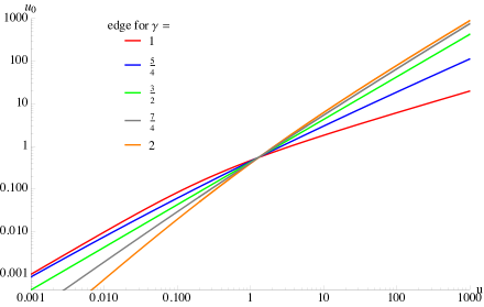
Figure 1: The value of the edge $u_{0}$ is plotted against $u$ in log-log space for $\beta=2$ and different values of $\gamma$.

We now use the two equivalent formulae obtained above for $\rho_{*}(b)$, where we insert $\phi(z)=(z)^{\gamma}_{+}$ which lead to equivalent forms that we give for completeness.

14.3 First form of the density

The optimal density reads

$$\begin{split}&\forall b\geq u,\quad\rho_{*}(b)=\frac{\sqrt{(b-u_{0})_{+}}}{\pi}+\frac{1}{2\pi}\frac{u_{0}}{(b-u)^{1/2}}\,_{2}F_{1}\left(\frac{1}{2},\gamma-\frac{1}{2};\gamma+\frac{1}{2};\frac{u-u_{0}}{u-b}\right)\\ &\forall b\leq u,\quad\rho_{*}(b)=\frac{\sqrt{(b-u_{0})_{+}}}{\pi}\left[1+\frac{4C_{\gamma}}{\beta\pi}(\gamma-\frac{1}{2})(u-b)^{\gamma-\frac{3}{2}}\,_{2}F_{1}\left(\frac{1}{2},\frac{3}{2}-\gamma;\frac{3}{2};\frac{b-u_{0}}{b-u}\right)\right]\end{split}$$ (144)

Proof.

From Eq. (97) we obtain using the explicit form for $f(u)$, see Eq. (122)

$$\rho_{*}(b)=\frac{\sqrt{(b-u_{0})_{+}}}{\pi}+\frac{2}{\beta\pi^{2}}\int_{0}^{w(u)}\frac{\mathrm{d}w^{\prime}}{\sqrt{(b-u+(\frac{w^{\prime}}{C_{\gamma}})^{\frac{1}{\gamma-1/2}})_{+}}}$$ (145)

where we recall that $w(u)$ is the unique positive root of Eq. (137). Performing the change of variable $w^{\prime}=C_{\gamma}|b-u|^{\gamma-1/2}z$ and using Eqs. (142) and (143), it can be written as (with $\epsilon={\rm sgn}(b-u)$)

$$\rho_{*}(b)=\frac{\sqrt{(b-u_{0})_{+}}}{\pi}+\frac{2C_{\gamma}}{\beta\pi^{2}}|b-u|^{\gamma-1}\int_{0}^{(\frac{u-u_{0}}{|b-u|})^{\gamma-1/2}}\frac{\mathrm{d}z}{\sqrt{(\epsilon+z^{\frac{1}{\gamma-1/2}})_{+}}}$$ (146)

For $b>u$ we can perform the integral (with $\epsilon=+1$) and we find

$$\rho_{*}(b)=\frac{\sqrt{(b-u_{0})_{+}}}{\pi}+\frac{2C_{\gamma}}{\beta\pi^{2}}\frac{(u-u_{0})^{\gamma-1/2}}{(b-u)^{1/2}}\,_{2}F_{1}\left(\frac{1}{2},\gamma-\frac{1}{2};\gamma+\frac{1}{2};\frac{u-u_{0}}{u-b}\right)$$ (147)

which, using (142) and (143) can be equivalently written as in (LABEL:dens11). For $b<u$ we calculate the same integral with $\epsilon=-1$), this gives

$$\rho_{*}(b)=\frac{\sqrt{(b-u_{0})_{+}}}{\pi}+\frac{2C_{\gamma}}{\beta\pi^{2}}(u-b)^{\gamma-1}\left(i\frac{(u-u_{0})^{\gamma-1/2}}{(u-b)^{\gamma-1/2}}\,_{2}F_{1}\left(\frac{1}{2},\gamma-\frac{1}{2};\gamma+\frac{1}{2};\frac{u-u_{0}}{u-b}\right)-\frac{i\sqrt{\pi}\Gamma\left(\gamma+\frac{1}{2}\right)}{\Gamma(\gamma)}\right)$$ (148)

A nicer equivalent form can be obtained by performing another equivalent integral. We rewrite the optimal density as

$$\rho_{*}(b)=\frac{\sqrt{(b-u_{0})_{+}}}{\pi}+\frac{2C_{\gamma}}{\beta\pi^{2}}|b-u|^{\gamma-1}(\gamma-\frac{1}{2})\int_{1}^{\frac{u-u_{0}}{u-b}}\rmd y\,\frac{y^{\gamma-3/2}}{\sqrt{y-1}}$$ (149)

which upon integration gives formula (LABEL:dens11). ∎

14.4 Second form of the density

Defining $\tau=\frac{u-u_{0}}{b-u_{0}}$, the optimal density reads

$$\begin{split}&\forall b\geq u,\quad\rho_{*}(b)=\frac{\sqrt{(b-u_{0})_{+}}}{\pi}\left[1+\frac{u_{0}}{2(b-u_{0})}~{}_{2}F_{1}(1,\frac{1}{2},\gamma+\frac{1}{2},\tau)\right]\\ &\forall b\leq u,\quad\rho_{*}(b)=\frac{\sqrt{(b-u_{0})_{+}}}{\pi}\left[1+\frac{(\gamma-\frac{1}{2})u_{0}}{u-u_{0}}~{}_{2}F_{1}(1,\frac{3}{2}-\gamma,\frac{3}{2},\frac{1}{\tau})\right]\end{split}$$ (150)

Proof.

We now use the formula (34) given in the Letter, i.e. (99) here. It leads to

$$\rho_{*}(b)=\frac{\sqrt{(b-u_{0})_{+}}}{\pi}\left[1+\frac{\gamma}{\beta\pi}\mathchoice{{\vbox{\hbox{$\textstyle-$}}\kern-4.86108pt}}{{\vbox{\hbox{$\scriptstyle-$}}\kern-3.25pt}}{{\vbox{\hbox{$\scriptscriptstyle-$}}\kern-2.29166pt}}{{\vbox{\hbox{$\scriptscriptstyle-$}}\kern-1.875pt}}\!\int_{-\infty}^{+\infty}\frac{\rmd b^{\prime}}{b+b^{\prime}-u}\frac{(b^{\prime})_{+}^{\gamma-1}}{\sqrt{(u-u_{0}-b^{\prime})_{+}}}\right]$$ (151)

We perform the change of variable $X=\sqrt{1-\frac{b^{\prime}}{u-u_{0}}}$ and $\tau=\frac{u-u_{0}}{b-u_{0}}$

$$\rho_{*}(b)=\frac{\sqrt{(b-u_{0})_{+}}}{\pi}\left[1+\frac{2\gamma}{\beta\pi}\frac{(u-u_{0})^{\gamma-\frac{1}{2}}}{b-u_{0}}\mathchoice{{\vbox{\hbox{$\textstyle-$}}\kern-4.86108pt}}{{\vbox{\hbox{$\scriptstyle-$}}\kern-3.25pt}}{{\vbox{\hbox{$\scriptscriptstyle-$}}\kern-2.29166pt}}{{\vbox{\hbox{$\scriptscriptstyle-$}}\kern-1.875pt}}\!\int_{0}^{1}\rmd X\,\frac{(1-X^{2})^{\gamma-1}}{1-\tau X^{2}}\right]$$ (152)

For $\tau\leq 1$, i.e. $b\geq u$, the integral is given by a hypergeometric function, leading to formula (150) upon simplification using Eqs. (122) and (143). It is equivalent to Eq. (147) using relations between hypergeometric functions, i.e for $\tau\leq 1$ one has ${}_{2}F_{1}(1,\frac{1}{2},\gamma+\frac{1}{2},\tau)=(1-\tau)^{-1/2}~{}_{2}F_{1}(\frac{1}{2},\gamma-\frac{1}{2};\gamma+\frac{1}{2};\frac{\tau}{\tau-1})$. For $\tau>1$, one uses the reflection formula for hypergeometric functions

$$\begin{split}~{}_{2}F_{1}(1,\frac{1}{2},\gamma+\frac{1}{2},\tau)&=\frac{2\gamma-1}{\tau}\!~{}_{2}F_{1}(1,\frac{3}{2}-\gamma,\frac{3}{2},\frac{1}{\tau})+\frac{\Gamma(\gamma+\frac{1}{2})\sqrt{\pi}}{\Gamma(\gamma)}(-\tau)^{-\frac{1}{2}}~{}_{2}F_{1}(\frac{1}{2},1-\gamma,\frac{1}{2},\frac{1}{\tau})\end{split}$$ (153)

Bearing in mind that Eq. (151) contains a principal part, that $\mathchoice{{\vbox{\hbox{$\textstyle-$}}\kern-4.86108pt}}{{\vbox{\hbox{$\scriptstyle-$}}\kern-3.25pt}}{{\vbox{\hbox{$\scriptscriptstyle-$}}\kern-2.29166pt}}{{\vbox{\hbox{$\scriptscriptstyle-$}}\kern-1.875pt}}\!\int\frac{1}{x}\underset{\varepsilon\to 0}{=}\int\Re(\frac{1}{x\pm i\varepsilon})$ and that the last term in Eq. (153) is purely imaginary, i.e. $(-\tau)^{-\frac{1}{2}}\in i\mathbb{R}$, we can discard the last term by taking the real part of Eq. (153) leading to the proposed continuation in Eq. (150). By the same transformation between hypergeometric functions evaluated at $\tau$ or $\tau/(\tau-1)$, we show the equivalence between the second equation of Eq. (150) with the second equation of Eq. (LABEL:dens11). ∎

14.5 Singularities of the density

The density is analytic everywhere except at $b=u_{0}$ (the edge) and at $b=u$ (the first point of application of the potential). The singularity for $b=u$ is a power law divergence for $1/2<\gamma<1$. From Eq. (146) one obtains

$$\begin{split}&\rho_{*}(b)\simeq\frac{2C_{\gamma}}{\beta\pi^{2}}|b-u|^{\gamma-1}\int_{0}^{+\infty}\frac{\rmd z}{\sqrt{(\epsilon+z^{\frac{1}{\gamma-1/2}})_{+}}}=D_{\gamma}^{\epsilon}|b-u|^{\gamma-1}\\ &D_{\gamma}^{+}=\frac{2C_{\gamma}}{\beta\pi^{2}}\frac{\Gamma(1-\gamma)\Gamma(\frac{1}{2}+\gamma)}{\sqrt{\pi}}=\frac{\gamma}{\pi\beta\sin(\gamma\pi)}\;,\;D_{\gamma}^{-}=-\frac{2C_{\gamma}}{\beta\pi^{2}}\frac{\sqrt{\pi}\Gamma(1-\gamma)}{\Gamma\left(\frac{1}{2}-\gamma\right)}=-\cos(\gamma\pi)D_{\gamma}^{+}\end{split}$$ (154)

where $\epsilon={\rm sgn}(b-u)$ and this power law divergence becomes a logarithmic singularity for $\gamma=1$. More generally one finds, for any $\gamma>1/2$, $\gamma\neq 1,2$, expanding (LABEL:dens11) on both sides of $b=u$

$$\rho_{*}(b)=\frac{\sqrt{(b-u_{0})_{+}}}{\pi}+D_{\gamma}^{\epsilon}|b-u|^{\gamma-1}+\frac{(2\gamma-1)u_{0}}{4\pi(\gamma-1)\sqrt{u-u_{0}}}+\frac{u_{0}\left(2\gamma-1\right)(u-b)}{8\pi(\gamma-2)\left(u-u_{0}\right){}^{3/2}}+\mathcal{O}(b-u)^{2}$$ (155)

Finally we verify that the singularity at $b=u_{0}$ is always of semi-circle type. More precisely we obtain

$$\rho_{*}(b)=\frac{\sqrt{(b-u_{0})_{+}}}{\pi}+\frac{u_{0}\left(2\gamma-1\right)\sqrt{(b-u_{0})_{+}}}{2\pi(u-u_{0})}+\frac{(4(2-\gamma)\gamma-3)u_{0}\left(b-u_{0}\right)_{+}^{3/2}}{6\pi\left(u-u_{0}\right)^{2}}+\mathcal{O}\left(b-u_{0}\right)^{\frac{5}{2}}$$ (156)

14.6 Hard wall limit for the optimal density

In the limit $B\to+\infty$ and for any $\gamma$, one recovers the result for the hard wall

$$\rho_{B=+\infty,u}(b)=\frac{2b-u}{2\pi\sqrt{(b-u)_{+}}}$$ (157)

Proof.

We recall that for $b\geq u$, the optimal density reads

$$\begin{split}\rho_{B,u}(b)&=\frac{\sqrt{(b-u_{0})_{+}}}{\pi}+\frac{1}{2\pi}\frac{u_{0}}{(b-u)^{1/2}}\,_{2}F_{1}\left(\frac{1}{2},\gamma-\frac{1}{2};\gamma+\frac{1}{2};\frac{u-u_{0}}{u-b}\right)\end{split}$$ (158)

The saddle point equation being $\frac{\beta\pi}{4}u_{0}=Bf(u-u_{0})$, we see that the hard wall limit, $B\to+\infty$, imposes that $u_{0}=u$. In this case, the optimal density reads

$$\begin{split}\rho_{B,u}(b)&=\frac{\sqrt{b-u}}{\pi}+\frac{1}{2\pi}\frac{u}{(b-u)^{1/2}}\,_{2}F_{1}\left(\frac{1}{2},\gamma-\frac{1}{2};\gamma+\frac{1}{2};0\right)\end{split}$$ (159)

As ${}_{2}F_{1}\left(\frac{1}{2},\gamma-\frac{1}{2};\gamma+\frac{1}{2};0\right)=1$, we obtain the hard wall density $\rho_{B=+\infty,u}(b)=\frac{2b-u}{2\pi\sqrt{(b-u)_{+}}}$. ∎

14.7 Optimal density for special values of $\gamma$ (for $B=1$)

• For $\gamma=3/2$, using $C_{\gamma}=3\pi/8$, $u=(1+\frac{2\beta}{3})u_{0}$ we find for all $b$ the remarkably simple expression

  $$\rho_{*}(b)=\left[\frac{\sqrt{b-u_{0}}}{\pi}+\frac{3}{2\beta\pi}(\sqrt{b-u_{0}}-\sqrt{(b-u)_{+}})\right]\theta(b-u_{0})$$ (160)

  

  Figure 2: Optimal density $\rho_{*}(-b)$ for the soft wall with $\gamma=3/2$ (solid line), compared to the semi-circle density $\rho_{\rm Ai}(-b)$ (dashed line). The external potential $\phi(u+b)$ is represented on the dotted line.

• For $\gamma=1$, using $C_{\gamma}=1$, $\frac{u_{0}}{\sqrt{u-u_{0}}}=\frac{4}{\beta\pi}$ we find for all $b$ the expression

  $$\rho_{*}(b)=\left[\frac{\sqrt{b-u_{0}}}{\pi}+\frac{2}{\beta\pi^{2}}\log\left(\frac{\sqrt{b-u_{0}}+\sqrt{u-u_{0}}}{\sqrt{|b-u|}}\right)\right]\theta(b-u_{0})$$ (161)

  which, upon simple manipulations, recovers the result obtained in Ref. [13] by a quite different calculation.

  

  (a) $u=25$

  

  (b) $u=0.05$

  Figure 3: Same as Fig. 2 for the linear wall $\gamma=1$ with $u=25$ and $u=0.05$. The optimal density for $u=0.05$ is also compared to the infinite hard-wall $\rho_{HW}(-b)$ showing a good agreement.

• For $\gamma=2$, we find

  $$\rho_{*}(b)=\left[\frac{\sqrt{b-u_{0}}}{\pi}+\frac{2}{\pi^{2}\beta}\bigg{(}2\sqrt{b-u_{0}}\sqrt{u-u_{0}}+(b-u)\log\mathinner{\!\left\lvert\frac{\sqrt{b-u_{0}}-\sqrt{u-u_{0}}}{\sqrt{b-u_{0}}+\sqrt{u-u_{0}}}\right\rvert}\bigg{)}\right]\theta(b-u_{0})$$ (162)

  

  (a) $u=100$

  

  (b) $u=1$

  Figure 4: Same as Fig. 2 for the quadratic wall $\gamma=2$ with $u=100$ and $u=1$.

• For $\gamma=5/2$ we find

  $$\rho_{*}(b)=\left[\frac{\sqrt{b-u_{0}}}{\pi}+\frac{5}{4\beta\pi}(\sqrt{b-u_{0}}(3(u-b)+(b-u_{0}))+2(b-u)_{+}^{3/2})\right]\theta(b-u_{0})$$ (163)

15 PDF $P({\sf L})$ for monomial walls

We study the PDF $P({\sf L})$ for monomial walls, $\phi(z)=(z)_{+}^{\gamma}$ and we first start with the case $\gamma=3/2$ where calculations are simple. Inserting the result for $\Sigma_{B\phi}$ of Eq. (132) into Eq. (107) we have

$$\tilde{G}(\tilde{L})=\max_{B}\left[\frac{\beta}{24}\frac{3B}{3B+2\beta}u^{3}-B\tilde{L}\right]$$ (164)

The optimal $B$ is given by $B=\dfrac{\beta}{6}(\dfrac{u^{3/2}}{\sqrt{\tilde{L}}}-4)$, which inserted into Eq. (164) gives

$$G(\tilde{L})=\frac{\beta}{24}(u^{3/2}-4\sqrt{\tilde{L}})^{2}\quad 0<\tilde{L}<\mathbb{E}_{\beta}[{\sf L}]=\frac{u^{3}}{16}$$ (165)

Hence, as given in the Letter $G(\ell)=\frac{\beta u^{3}}{24}(1-\sqrt{\ell})^{2}$. Near the typical value $\ell=1$, the rate function takes the form

$$G(\ell)\simeq\frac{(\ell-1)^{2}}{2\sigma}\quad,\quad\sigma=\frac{48}{\beta u^{3}}$$ (166)

which consistent with the first two cumulants, $\kappa_{1}(u)=-\frac{1}{16}u^{3}$ and $\kappa_{2}(u)=\frac{3}{16\beta}u^{3}$.

For $\gamma\neq 3/2$, let us first recall the cumulants $\mathbb{E}_{\beta}[{\sf L}^{n}]^{c}=t^{2}(-1)^{n}\tilde{\kappa}_{n}(u)$, for $n=1,2$

$$\mathbb{E}_{\beta}[{\sf L}]=t^{2}k_{1}u^{\gamma+\frac{3}{2}}\quad,\quad k_{1}=\frac{\Gamma(\gamma+1)}{2\sqrt{\pi}\Gamma(\gamma+\frac{5}{2})}=-\frac{1}{\pi}\frac{C_{\gamma}}{(\gamma+\frac{3}{2})(\gamma+\frac{1}{2})}$$ (167)

$$\mathbb{E}_{\beta}[{\sf L}^{2}]^{c}=t^{2}k_{2}u^{2\gamma}\quad,\quad k_{2}=\frac{2}{\beta\pi^{2}\gamma}C_{\gamma}^{2}$$ (168)

We can now use the scaling relations (124) and (125) to write

$$\tilde{G}(\tilde{L})=\max_{B}\left[(\frac{2}{\beta})^{\frac{3+2\gamma}{3-2\gamma}}B^{\frac{6}{3-2\gamma}}\Sigma_{\phi}\left(uB^{-\frac{2}{3-2\gamma}}(\frac{\beta}{2})^{\frac{2}{3-2\gamma}}\right)-B\tilde{L}\right]$$ (169)

Let us denote $U=u(\frac{\beta}{2})^{\frac{2}{3-2\gamma}}B^{-\frac{2}{3-2\gamma}}$ and insert $\tilde{L}=k_{1}u^{\gamma+\frac{3}{2}}\ell$ so that

$$G(\ell)=\frac{\beta}{2}u^{3}\max_{U}[U^{-3}\Sigma_{\phi}(U)-k_{1}U^{\gamma-3/2}\ell]$$ (170)

where here and below $\Sigma_{\phi}=\Sigma_{\phi}^{\beta=2}$. The rate function is determined by the parametric system

$$G(\ell)=\frac{\beta}{2}u^{3}(U^{-3}\Sigma_{\phi}(U)-k_{1}U^{\gamma-3/2}\ell)$$ (171)

$$3\Sigma_{\phi}(U)-U\Sigma^{\prime}_{\phi}(U)=(\frac{3}{2}-\gamma)k_{1}U^{\gamma+3/2}\ell$$ (172)

$$G^{\prime}(\ell)=-k_{1}U^{\gamma-3/2}$$ (173)

Note that, remarkably, for any $\gamma$ the only dependence in $u$ and $\beta$ is in the cubic prefactor $\beta u^{3}$ as noted in the Letter. In the vicinity of the typical value, the fluctuations are Gaussian and given by

$$G(\ell)\simeq\frac{(\ell-1)^{2}}{2\sigma}\quad,\quad\sigma=\frac{\tilde{\kappa}_{2}(u)}{\tilde{\kappa}_{1}(u)^{2}}=\frac{2}{\beta}\frac{(\gamma+\frac{3}{2})^{2}(\gamma+\frac{1}{2})^{2}}{u^{3}}$$ (174)

16 Exponential walls $\phi(z)=e^{z}$

Until now we considered $\phi$ in $\Omega_{0}$, with $\phi(z\leq 0)=0$. It is possible to extend our formula to a larger class of soft walls, $\Omega_{1}$, such that $\phi$ is still positive and increasing but does not vanish on $\mathbb{R}^{-}$, instead it vanishes smoothly as $z\to-\infty$. The bounds of the integrals over $u$ have to be taken at $u=-\infty$ and the formula go through.

16.1 $\Sigma_{\phi}(u)$ for the exponential wall

Consider the following linear statistics

$${\sf L}_{c,B}(t,u)=Bt\sum_{i}e^{c(u+t^{-2/3}a_{i})}$$ (175)

we first note that by rescaling of $t$ and $u$ we have ${\sf L}_{c,B}(t,u)={\sf L}_{1,1}(c^{-3/2}t,cu+\log(Bc^{3/2}))$, hence it is sufficient to study the case $c=1,B=1$ since the $c,B$ dependence can be restored easily. The function $f(u)$ and the saddle point SP1 are then

$$f(u)=\frac{1}{2}\int_{0}^{+\infty}\frac{\rmd b}{\sqrt{b}}e^{u-b}=\frac{\sqrt{\pi}}{2}e^{u}\qquad,\qquad w=f(u-\frac{4}{\beta\pi}w)=\frac{\sqrt{\pi}}{2}e^{u-\frac{4}{\beta\pi}w}$$ (176)

We obtain the solution of SP1 in terms of the principal branch of the Lambert function $W_{0}$ [16]

$$w(u)=\frac{\beta\pi}{4}W_{0}(\frac{2e^{u}}{\beta\sqrt{\pi}})$$ (177)

We calculate the excess energy using the formula $\Sigma_{\phi}(u)=\frac{1}{\pi}\int_{-\infty}^{u}\rmd u^{\prime}w(u^{\prime})[u-u^{\prime}]$

$$\Sigma_{\phi}(u)=\frac{\beta}{48}(2W^{3}+9W^{2}+12W)\quad,\quad W\mathrel{\mathop{\mathchar 58\relax}}=W_{0}\left(\frac{2e^{u}}{\beta\sqrt{\pi}}\right)$$ (178)

It is useful to note that the derivative of the express energy reads

$$\Sigma^{\prime}_{\phi}(u)=\frac{1}{\pi}\int_{-\infty}^{u}\rmd u^{\prime}\,w(u^{\prime})=\frac{\beta}{8}(2W+W^{2})$$ (179)

The different asymptotics are

$$\begin{split}&w(u)\underset{u\to-\infty}{\simeq}\frac{\sqrt{\pi}}{2}\,e^{u}+\mathcal{O}(e^{2u})\quad,\quad w(u)\underset{u\to+\infty}{\simeq}\frac{\pi\beta}{4}\left[u+\log(\frac{2}{\sqrt{\pi}\beta u})+\mathcal{O}(\frac{\log u}{u})\right]\\ &\Sigma_{\phi}(u)\underset{u\to-\infty}{\simeq}\frac{e^{u}}{2\sqrt{\pi}}+\mathcal{O}(e^{2u})\;,\quad\Sigma_{\phi}(u)\underset{u\to+\infty}{\simeq}\frac{\beta u^{3}}{24}+\frac{\beta u^{2}}{16}\log\left(\frac{4e^{2/3}}{\pi\beta^{2}u^{2}}\right)+\mathcal{O}(u\log(u)^{2})\end{split}$$ (180)

16.2 Optimal density for the exponential wall

The associated optimal density has a support $[u_{0},+\infty[$ with $u_{0}>0$ given by $u_{0}=\frac{4}{\beta\pi}w(u)=W_{0}(\frac{2}{\beta\sqrt{\pi}}e^{u})$ and is given by

$$\rho_{*}(b)=\frac{\sqrt{(b-u_{0})_{+}}}{\pi}+\frac{2}{\beta\pi^{2}}\int_{0}^{w(u)}\frac{\mathrm{d}w^{\prime}}{\sqrt{(b-u+f^{-1}(w^{\prime}))_{+}}}$$ (181)

Let us calculate the second term

$$\int_{0}^{w(u)}\frac{\mathrm{d}w^{\prime}}{\sqrt{(b-u+f^{-1}(w^{\prime}))_{+}}}=\int_{0}^{w(u)}\frac{\mathrm{d}w^{\prime}}{\sqrt{(b-u+\log\frac{2w^{\prime}}{\sqrt{\pi}})_{+}}}$$ (182)

$$=\frac{\sqrt{\pi}}{2}\int_{u-b}^{u-u_{0}}\mathrm{d}u^{\prime}\frac{e^{u^{\prime}}}{\sqrt{b-u+u^{\prime}}}=\frac{\pi e^{u-b}}{2}\text{Erfi}\left(\sqrt{b-u_{0}}\right)$$ (183)

where we have defined $u^{\prime}=\log\frac{2w^{\prime}}{\sqrt{\pi}}$ and used that $\log\frac{2w(u)}{\sqrt{\pi}}=u-\frac{4}{\beta\pi}w(u)=u-u_{0}$. Since there is a relation between $u$ and $u_{0}$, $e^{u}=\frac{\beta\sqrt{\pi}}{2}u_{0}\,e^{u_{0}}$, we can express the optimal density $\rho_{*}(b)$ only in terms of $u_{0}$ leading to

$$\begin{split}\rho_{*}(b)&=\frac{\sqrt{(b-u_{0})_{+}}}{\pi}+\frac{u_{0}\,e^{u_{0}-b}}{2\sqrt{\pi}}\text{Erfi}\left(\sqrt{b-u_{0}}\right)\end{split}$$ (184)

The optimal density is plotted in Fig. 6 for $u=20$ and $u=1$. We see that for large $u$, the density becomes close to the hard wall one, while for small $u$ the reorganization of the density is perturbative.

Figure 5: Edge of the exponential wall for $\beta=2$ as a function of $u$. For large $u$, $u_{0}\simeq u$.

(a) $u=20$

(b) $u=1$

Figure 6: Optimal density $\rho_{*}(-b)$ for the exponential wall (solid line), compared to the semi-circle density $\rho_{\rm Ai}(-b)$ (dashed line) for $u=20$ and $u=1$. The potential $\phi(u+b)$ is represented with the dotted line.

16.3 PDF $P({\sf L})$ for the exponential wall

Let us first note that for the exponential wall the first cumulant is

$$\mathbb{E}_{\beta}[L]=\frac{t^{2}}{\pi}\int_{0}^{+\infty}\rmd b\,\sqrt{b}e^{u-b}=\frac{e^{u}}{2\sqrt{\pi}}t^{2}$$ (185)

Now, it is easy to see that for the exponential wall $\Sigma_{B\phi}(u)=\Sigma_{\phi}(u+\log B)$ which allows to calculate easily the PDF of ${\sf L}$, indeed defining $\hat{u}=u+\log B$, we have

$$G(\ell)=\max_{B}\left[\Sigma_{\phi}(u+\log B)-\frac{e^{u}}{2\sqrt{\pi}}B\ell\right]=\max_{\hat{u}}\left[\Sigma_{\phi}(\hat{u})-\frac{e^{\hat{u}}}{2\sqrt{\pi}}\ell\right]$$ (186)

$G(\ell)$ is independent of $u$ and is given by the parametric system of equations

$$\begin{split}&G(\ell)=\Sigma_{\phi}(\hat{u})-\frac{e^{\hat{u}}}{2\sqrt{\pi}}\ell\qquad,\qquad\Sigma^{\prime}_{\phi}(\hat{u})=\frac{e^{\hat{u}}}{2\sqrt{\pi}}\ell\end{split}$$ (187)

Using the results of the previous subsection (Eqs. (178) and (179)) for $\Sigma_{\phi}$ and $\Sigma^{\prime}_{\phi}$ in terms of the variable

$$W\mathrel{\mathop{\mathchar 58\relax}}=W_{0}(\frac{2e^{\hat{u}}}{\beta\sqrt{\pi}})\quad\Longleftrightarrow\quad\frac{2e^{\hat{u}}}{\beta\sqrt{\pi}}=We^{W}$$ (188)

we obtain the system

$$\begin{split}G(\ell)=\frac{\beta}{48}W^{2}(2W+3)\qquad,\qquad\ell=\frac{1}{2}(2+W)e^{-W}\end{split}$$ (189)

and $G^{\prime}(\ell)=-\frac{\beta}{4}We^{W}$. The typical value therefore corresponds to $W=0$ and $\ell=1$. We solve the second equation in (189) by writing it as $-(2+W)e^{-(2+W)}=-2\ell e^{-2}$ so that

$$-(2+W)=W_{-1}(-2\ell e^{-2})$$ (190)

where one needs to take the second branch of the Lambert function to recover that $\ell=1$ is realized for $W=0$. This leads to our final result, for $\ell\leq 1$

$$G(\ell)=-\frac{\beta}{48}(2+W_{-1}(-2\ell e^{-2}))^{2}(1+2W_{-1}(-2\ell e^{-2}))$$ (191)

which is positive, as required, with its minimum at $\ell=1$.

• Near $\ell=1$,

  $$G(\ell)=\beta\left[\frac{1}{4}(\ell-1)^{2}-\frac{1}{3}(\ell-1)^{3}+\frac{1}{3}(\ell-1)^{4}+\mathcal{O}((\ell-1)^{5})\right]$$ (192)

• Near $\ell=0$,

  $$G(\ell)=\frac{\beta}{24}\left[-\log^{3}(\ell)+\frac{\log^{2}(\ell)(3+6\log(-\frac{\log\ell}{\log 2})}{2}+\mathcal{O}(\log(\ell)\log(-\log\ell)^{2})\right]$$ (193)

Again, here we have access only to the side $\ell\leq 1$, the side $\ell>1$ requires to be able to treat the case of negative $B$, which goes beyond this Letter.

17 Inverse monomial walls $\phi(z)=(-z)^{-\delta}$, $\delta>3/2$

Another example of functions in the set $\Omega_{1}$ are the inverse monomial walls

$$\phi(z)=(-z)^{-\delta}\quad b<0\quad,\quad\phi(z)=+\infty\quad z>0$$ (194)

such that $\phi(u+t^{-2/3}a_{i})$ has an infinite hard wall for $t^{-2/3}a_{i}>-u$, which penetrates the semi-circle as a power law for $t^{-2/3}a_{i}<-u$. For $u>0$ the infinite hard wall part penetrates the semi-circle, while for $u<0$ it does not. The influence of the wall can be felt for any $u\in\mathbb{R}$ although it becomes weaker and weaker for a distant wall at large negative $u$ (see Fig. 7).

Figure 7: Representation of an inverse monomial wall with $\delta=2$ and of the density of the unperturbed Coulomb gas $\rho_{\rm Ai}$.

Since $a_{i}\sim-i^{2/3}$ for large $i$, we see that one must take $\delta>3/2$ for $L$ to be a convergent sum. The function $f(u)$ is given for $u<0$ as

$$f(u)=\frac{1}{2}\int_{0}^{+\infty}\frac{\rmd b}{\sqrt{b}}\frac{\delta}{(b-u)^{\delta+1}}=\frac{D_{\delta}}{(-u)^{\delta+\frac{1}{2}}}\quad,\quad D_{\delta}=\frac{\sqrt{\pi}\Gamma(\delta+\frac{1}{2})}{2\Gamma(\delta)}$$ (195)

with $f(u>0)=+\infty$. We must thus solve

$$w=\frac{D_{\delta}}{(-u+\frac{4}{\beta\pi}w)^{\delta+\frac{1}{2}}}\Longleftrightarrow u=\frac{4}{\beta\pi}w-(\frac{D_{\delta}}{w})^{\frac{1}{\delta+1/2}}$$ (196)

There is a unique positive solution $w=w(u)$ (since $\phi\in\Omega_{1}\subset\Omega_{2}$) increasing function of $u\in\mathbb{R}$, with

• $w(u)\simeq\frac{D_{\delta}}{(-u)^{\delta+\frac{1}{2}}}$ for large negative $u$ (distant wall),

• $w(u)\simeq\frac{\beta\pi}{4}u$ for large positive $u$.

The SAO/WKB SP1 saddle point is then $v(x)=\frac{4}{\beta\pi}w(u-x)$ for $x>0$ and is now non-zero and decreasing on $\mathbb{R}^{+}$ and decaying at large $x$ as $v(x)\simeq\frac{4}{\beta\pi}\frac{C_{\delta}}{x^{\delta+\frac{1}{2}}}$. For the excess energy $\Sigma_{\phi}(u)=\frac{\beta}{4}\int_{0}^{+\infty}\rmd x\,xv(x)$ to be finite, we need $\delta>3/2$ as anticipated above. We can use the following formula to obtain the expression of the excess energy

$$\Sigma_{\gamma}(u)=\frac{1}{2\pi}\int_{0}^{w(u)}\rmd w^{\prime}[u(w^{\prime})-u]^{2}=\frac{1}{2\pi}\int_{0}^{w(u)}\rmd w^{\prime}[\frac{4}{\beta\pi}w^{\prime}-(\frac{D_{\delta}}{w^{\prime}})^{\frac{1}{\delta+1/2}}-u]^{2}$$ (197)

Performing the integral and replacing all $(\frac{D_{\delta}}{w})^{\frac{2}{2\delta+1}}$ factors by $\frac{4}{\beta\pi}w-u$, we find

$$\begin{split}\Sigma_{\gamma}(u)&=\frac{w(u)\left(12\pi^{2}\beta^{2}\delta u^{2}-3\pi\beta(2\delta+3)(6\delta-1)uw(u)+4(2\delta-1)(2\delta+3)^{2}w^{2}(u)\right)}{3\pi^{3}\beta^{2}\delta(2\delta-3)(2\delta-1)}\\ \end{split}$$ (198)

The asymptotic behavior of the excess energy is

• $\Sigma_{\phi}(u)=\frac{\Gamma\left(\delta-\frac{3}{2}\right)}{2\sqrt{\pi}\Gamma(\delta)}\frac{1}{(-u)^{\delta-\frac{3}{2}}}$ for large negative $u$ (distant wall),

• $\Sigma_{\phi}(u)=\frac{\beta}{24}u^{3}$ for large positive $u$.

17.1 Upper and lower bounds on the excess energy

The inverse monomial walls $\phi(z)$ are larger then the hard wall potential $\phi_{\rm HW}$ implying the lower bound on the excess free energy

$$\forall u\geq 0,\qquad\Sigma_{\phi}(u)\geq\frac{\beta}{24}u^{3}$$ (199)

Besides, by the Jensen (first cumulant) inequality, we have

$$\forall u\leq 0,\quad\Sigma_{\phi}(u)\leq\frac{\Gamma\left(\delta-\frac{3}{2}\right)}{2\sqrt{\pi}\Gamma(\delta)}\frac{1}{(-u)^{\delta-\frac{3}{2}}}$$ (200)

18 Relation to truncated linear statistics: matching bulk and edge

In this Section we show that there is a smooth matching between the results of Ref. [14] for truncated linear statistics in the bulk and our results at the edge for the linear wall $\gamma=1$. The details of the matching are non-trivial and instructive. Furthemore we show universality, i.e. for any linear statistics smooth at a soft edge we obtain, up to coefficients, the same results corresponding to ours for $\gamma=1$.

18.1 Summary of results in the bulk

Let us first recall briefly the results of Ref. [14]. We use most of their notations. They study, for large $N$

$${\cal L}=\sum_{i=1}^{N_{1}}f(\lambda_{i})\quad,\quad f(\lambda)=\sqrt{\lambda}\quad,\quad\kappa=\frac{N_{1}}{N}$$ (201)

where the sum is over the $N_{1}$ largest eigenvalues of the Laguerre ensemble, which can be written as $\lambda_{i}=Nx_{i}$. Let us define the general density of eigenvalues in the bulk as $\hat{\rho}(x)=N^{-1}\sum_{i=1}^{N}\delta(x-x_{i})$, i.e. with unit normalization. For the Laguerre ensemble at large $N$ this density converges to the Marchenko-Pastur distribution $\hat{\rho}(x)=\rho_{\rm MP}(x)=\frac{1}{2\pi}\sqrt{\frac{4-x}{x}}$, which has a soft edge at $x=4$ with locally a semi-circle form. In Ref [14] the scaling $N_{1}/N=\kappa$ fixed was studied. The question is whether for small $\kappa$ one is able to match to the edge problem studied here.

From the replacement $\lambda_{i}=Nx_{i}$ one sees that for $f(\lambda)=\sqrt{\lambda}$ the typical size of the sum is of order $N^{3/2}$ (for $\kappa>0$), hence the authors introduced the random variable $s={\cal L}/N^{3/2}$ and obtained the following large deviation form for the probability of $s$, at fixed $\kappa$

$$P_{\kappa}(s)\sim\exp\left(-{\frac{\beta N^{2}}{2}}\Phi_{\kappa}(s)\right)$$ (202)

The typical (and mean) value for $s$, denoted $s_{0}(\kappa)$, such that $\Phi_{\kappa}(s_{0}(\kappa))=0$, is obtained simply by noting that for large $N$ there is a well defined level $c_{0}$ in $x$ which corresponds to $\kappa$, and by eliminating $c_{0}$ in the system

$$s_{0}=\int_{c_{0}}^{4}\sqrt{x}\rho_{\rm MP}(x)\quad,\quad\kappa=\int_{c_{0}}^{4}\rho_{\rm MP}(x)$$ (203)

Let us recall here the result for small $\kappa$, to the order relevant for us

$$s_{0}(\kappa)=2\kappa-\frac{3(3\pi)^{2/3}}{10\times 2^{1/3}}\kappa^{5/3}+\dots$$ (204)

where the $2\kappa$ comes simply from $\sqrt{x_{\rm edge}}=2$.

The authors of Ref. [14] write the JPDF of the eigenvalues $x_{i}$ as $\sim\exp(-{\frac{\beta N^{2}}{2}}{\cal E}[\hat{\rho}])$ where ${\cal E}[\hat{\rho}]$ is the standard logarithmic Coulomb Gas in the bulk. We have here generalized their calculation to arbitrary $\beta$, which is immediate. In addition to the usual constraint $\int\rmd x\hat{\rho}(x)=1$, they impose

$$\int_{c}^{d}\rmd x\hat{\rho}(x)=\kappa\quad,\quad\int_{c}^{d}\rmd x\sqrt{x}\hat{\rho}(x)=s$$ (205)

where $d$ is the upper edge of the support of $\rho$. They add Lagrange multiplier terms, ${\cal E}[\hat{\rho}]\to{\cal E}[\hat{\rho}]+\mu_{1}(\int_{c}^{d}\rmd x\sqrt{x}\hat{\rho}(x)-s)$ and similarly for the two other conditions (see their equation (3.8)). They then look for the minimal energy configuration, in the ensemble with fixed $\kappa,s$, which we denote $\hat{\rho}(x)=\rho_{\kappa,s}(x)$.

Here we discuss only the side $s<s_{0}(\kappa)$, relevant for us, and where the density has a single interval support. They find the optimal density

$$\rho_{\kappa,s}(x)=\frac{1}{2\pi}\sqrt{\frac{d-x}{x}}+\frac{4-d}{8\pi\sqrt{d-c}\sqrt{x}}\log\frac{\sqrt{d-c}+\sqrt{d-x}}{|\sqrt{d-c}-\sqrt{d-x}|}$$ (206)

where the three parameters $c,d,\mu_{1}$ are determined at the optimum by the three equations (3.35), (3.36) and (3.37) there, as a function of $\kappa,s$. The last two equations simply express the constraints (205). The large deviation function $\Phi_{\kappa}(s)$ is determined from integrating the relation

$$\Phi^{\prime}_{\kappa}(s)=-\mu_{1}$$ (207)

where $\mu_{1}=\mu_{1}(s,\kappa)$. No closed form was found but $\Phi_{\kappa}(s)$ was determined perturbatively near $s_{0}(\kappa)$ and for $s\to 0$. The optimal density (206) is strikingly similar to the one obtained here for the linear wall $\gamma=1$ (i.e. the result related to the KPZ large deviations first obtained in [13]). We now explain why, and give the connection between the two sets of results.

18.2 Connecting bulk truncated linear statistics and the soft wall at the edge

Let us start from the bulk, and consider a general linear statistics in the limit to the edge, $\kappa=N_{1}/N\to 0$. From the universality of the soft edge, the eigenvalues very near the edge take the form $\lambda_{i}=4N+\alpha a_{i}N^{1/3}$ for some constant $\alpha$, where the $\{a_{i}\}$ forms the $\beta$ Airy point process. For the case studied in Ref [14] it is easy to see that $\alpha=4^{2/3}$. We can thus write heuristically, for large $N$

$${\cal L}=\sum_{i=1}^{N_{1}}f(4N+\alpha a_{i}N^{1/3})=N_{1}f(4N)+\alpha N^{1/3}f^{\prime}(4N)\sum_{i=1}^{N_{1}}a_{i}+\frac{1}{2}\alpha^{2}N^{2/3}f^{\prime\prime}(4N)\sum_{i=1}^{N_{1}}a_{i}^{2}+\dots$$ (208)

while the first two terms are certainly present, the last term (neglected below) may not be the only subdominant one, but it is sufficient to illustrate our argument. For $f(\lambda)=\sqrt{\lambda}$ we see that

$${\cal L}=2N^{1/2}N_{1}+\frac{\alpha}{4N^{1/6}}\sum_{i=1}^{N_{1}}a_{i}-\frac{\alpha^{2}}{64N^{5/6}}\sum_{i=1}^{N_{1}}a_{i}^{2}+\dots$$ (209)

For $N_{1}$ large we can use that the ordered $a_{i}\simeq-(3\pi/2)^{2/3}i^{2/3}$ at large $i$, and obtain the typical value

$${\cal L}_{typ}=2N^{1/2}N_{1}-\frac{3\alpha(3\pi/2)^{2/3}}{20N^{1/6}}N_{1}^{5/3}+\mathcal{O}(N^{-5/6}N_{1}^{7/3})$$ (210)

Inserting $N_{1}=\kappa N$ and $\alpha=4^{2/3}$ it correctly reproduces the first two terms in the expansion (204) of $s_{0}(\kappa)$ at small $\kappa$ of [14]. This already suggests a smooth matching to the edge, since here we used the Airy point process, at least at the level of typical fluctuations. Note however that all terms are of the same order $N^{3/2}$ and the only perturbative parameter is thus small $\kappa$, which suggests that the higher order terms can be dropped.

On the other hand for $N_{1}$ large but fixed, taking $N$ to infinity first, we see that the successive terms in the expansion become smaller and smaller, and that the only remaining fluctuating term is linear in the Airy point process

$$\alpha N^{1/3}f^{\prime}(4N)\sum_{i=1}^{N_{1}}a_{i}$$ (211)

which is similar to the one which we studied for the monomial wall with $\gamma=1$, i.e. $\phi(z)=(z)_{+}$ with the correspondence indicated in the Letter, that the typical $N_{1}\simeq\frac{2u^{3/2}}{3\pi}t$ (both $N_{1}$ and $t$ large). Let us now make this more precise. We want to compare the bulk random variable $s$ studied in [14] (first line) and the edge random variable $\tilde{L}$ studied here (second line)

$$s=2\kappa+4^{-1/3}N^{-5/3}\sum_{i=1}^{N_{1}}a_{i}$$ (212)

$$\tilde{L}=t^{-2}{\sf L}=t^{-1}\sum_{i}(u+t^{-2/3}a_{i})_{+}\simeq u\frac{K}{t}+t^{-5/3}\sum_{i=1}^{K}a_{i}$$ (213)

We must be careful that the first problem was studied at fixed $s,\kappa=\frac{N_{1}}{N}$, while the second is studied at fixed $u$, and that here $K$ is the cut-off defined by $a_{K}\approx-t^{2/3}u$, i.e. the largest index for which $u+t^{-2/3}a_{i}>0$, so it is a priori a fluctuating quantity. To connect the two, we want to identify $K=N_{1}$ although the ensembles may be different. It turns out that it works, and that for large $N_{1},t$ at fixed $N_{1}/t$ one can perform this identification, in the way described below.

Thus, to summarize, we want to identify , at small $\kappa$

$$s-s_{0}(\kappa)=4^{-1/3}(\frac{t}{N})^{5/3}(\tilde{L}-\tilde{L}_{typ})$$ (214)

A first check is to calculate the variance of both sides. Using the result for the variance of $s$ in (4.9) of [14] we obtain for small $\kappa$

$${\rm Var}(s)\simeq\frac{2}{\beta}\frac{(6\pi\kappa)^{4/3}}{16\pi^{2}N^{2}}=4^{-2/3}\frac{2}{\beta}(\frac{t}{N})^{10/3}\frac{u^{2}}{\pi^{2}t^{2}}=4^{-2/3}(\frac{t}{N})^{10/3}{\rm Var}(\tilde{L})$$ (215)

consistent with Eqs. (29) and (167). In the middle equality we have replaced $N_{1}$ by $K_{typ}$ where $K_{typ}$ is determined by

$$\int_{0}^{u}\rmd b\,\rho_{\rm Ai}(b)=\frac{K_{typ}}{t}\quad\Leftrightarrow\quad\frac{K_{typ}}{t}=\frac{2}{3\pi}u^{3/2}$$ (216)

This is consistent with (214).

However, if one now calculates the third cumulant on both sides one finds that it fails by a factor of $4$. The reason is that the two ensembles (fixed $\kappa$ and fixed $u$) are not identical, and must be related by a transformation which we describe below. Hence the identification (214) is subtle, although the final correct version is quite natural, as shown below. In a nutshell the idea is that, conditionned to a very atypical value of $s$, or of $\tilde{L}$, the optimal density deviates from the unperturbed semi-circle $\rho_{\rm Ai}(b)$, hence the relation of $N_{1}/t$ to $u$ changes.

18.3 Recalling results for $\gamma=1$

Before working it out, it is useful to recall the full set of results for the monomial wall $\gamma=1$, $\phi(z)=(z)_{+}$. We will indicate by an index $B$ the result for $\phi\to B\phi$ since we need the amplitude $B$ to probe all values for $\tilde{L}$ by Legendre transform. The associated functions $f_{B}(u)$ and $w(u)=w_{B}(u)$ solving Eq. (15) of the Letter are

$$f_{B}(u)=B\sqrt{(u)_{+}}\quad,\quad u^{B}_{0}={\frac{4}{\beta\pi}w_{B}(u)=\frac{8B^{2}}{\pi^{2}\beta^{2}}(\sqrt{1+\frac{\beta^{2}\pi^{2}}{4B^{2}}u}-1)}$$ (217)

leading to the excess energy which we call $\Sigma_{B}(u)$, and its scaling form

$$\Sigma^{(\beta=2)}_{B=1}(u)\mathrel{\mathop{\mathchar 58\relax}}=\Sigma(u)=\frac{4\left(\pi^{2}u+1\right)^{5/2}}{15\pi^{6}}-\frac{u^{2}}{2\pi^{2}}-\frac{2u}{3\pi^{4}}-\frac{4}{15\pi^{6}}\;\;,\;\;{\Sigma^{(\beta)}_{B}(u)=B^{6}(\frac{2}{\beta})^{5}\Sigma(u(\frac{\beta}{2B})^{2})}$$ (218)

The optimal density and its scaling property read

$$\rho^{(\beta)}_{*,B,u}(b)=\frac{\sqrt{b-u_{0}}}{\pi}+\frac{B}{\beta\pi^{2}}\log\frac{\sqrt{u-u_{0}}+\sqrt{b-u_{0}}}{|\sqrt{u-u_{0}}-\sqrt{b-u_{0}}|}\quad,\quad u_{0}=u_{0}^{B}$$ (219)

$$\frac{\beta\pi}{4B}u^{B}_{0}=\sqrt{u-u^{B}_{0}}\quad,\quad\rho^{(\beta)}_{*,B,u}(b)=\frac{2B}{\beta}\rho^{(2)}_{*,1,u(\frac{\beta}{2B})^{2}}(b(\frac{\beta}{2B})^{2})$$ (220)

18.4 Matching bulk and edge

The optimal edge density (219) is strikingly similar to the optimal bulk density (206) near the soft edge, $x,d,c\approx 4$. More precisely if we write

$$d=4-\epsilon u^{B}_{0}\quad,\quad x=4-\epsilon b\quad,\quad c=4-\epsilon u\quad,\quad\sqrt{d-c}=\sqrt{\epsilon}\sqrt{u-u^{B}_{0}}$$ (221)

then (206) becomes, using $\sqrt{u-u_{0}^{B}}=\frac{\beta\pi}{4B}u_{0}^{B}$, for small $\epsilon$

$$\rho_{\kappa,s}(x)\simeq\frac{\sqrt{\epsilon}}{4}\rho^{*}_{B,u}(b)$$ (222)

The factor $\epsilon$ which relates the volume elements, $\rmd x=\epsilon\rmd b$, can be predicted from the edge behavior of the rescaled eigenvalues $x_{i}=\lambda_{i}/N$

$$\rmd x_{i}=\frac{\alpha}{N^{2/3}}\rmd a_{i}=\alpha(\frac{t}{N})^{2/3}\rmd b_{i}$$ (223)

with here $\alpha=4^{2/3}$ hence

$$\epsilon=(\frac{4t}{N})^{2/3}=(\frac{4t}{N_{1}})^{2/3}\kappa^{2/3}$$ (224)

The number of eigenvalues in interval $\rmd x$ is equal to the one in $\rmd b$, hence, from our definitions, $N\hat{\rho}(x)\rmd x=t\rho(b)\rmd b$. Using $\rmd x=\epsilon\rmd b$ and (224) explains the prefactor in the correspondence (222).

We now justify the equations (221), and give the correspondence between parameters $\kappa,s$ and $B,u$. We also derive the relation between our function $\Sigma_{\phi}(u)$ and the results of [14]. Let us now write the equations (3.35), (3.36) and (3.37) in the limit $\kappa\to 0$. Let us define $d=4-\epsilon d_{1}$, $c=4-\epsilon c_{1}$, then these equations become, discarding terms of higher orders in $\epsilon$

$$\kappa=\frac{\sqrt{c_{1}-d_{1}}}{24\pi}(4c_{1}-d_{1})\epsilon^{3/2}$$ (225)

$$s-2\kappa=\frac{\sqrt{c_{1}-d_{1}}\left(d_{1}^{2}-2c_{1}d_{1}-4c_{1}^{2}\right)}{160\pi}\epsilon^{5/2}$$ (226)

$$\mu_{1}=\frac{\pi}{2}\frac{d_{1}}{\sqrt{c_{1}-d_{1}}}\epsilon^{1/2}$$ (227)

So one must calculate the $\mathcal{O}(1)$ parameters $c_{1}$ and $d_{1}$ as functions of $s$ and $\kappa$, obtain $\mu_{1}(\kappa,s)$ from the last equation, and finally obtain the large deviation for the probability by integration

$$\Phi_{\kappa}(s)=-\int_{s_{0}(\kappa)}^{s}\mu_{1}(\kappa,s)\rmd s$$ (228)

at fixed $\kappa$. The typical value $s_{0}(\kappa)$ in (204) is recovered and corresponds to $d_{1}=\mu_{1}=0$. It is easy to see that $\Phi_{\kappa}(s)$ then takes the scaling form in the small $\kappa$ limit (i.e. small $\epsilon$)

$$\Phi_{\kappa}(s)=\kappa^{2}\hat{\Phi}(S)\quad,\quad S=\kappa^{-5/3}(s-s_{0}(\kappa))$$ (229)

To calculate $\hat{\Phi}(S)$ we proceed as follows. Define $\tilde{\kappa}=\kappa\epsilon^{-3/2}$. Set $\sqrt{c_{1}-d_{1}}=y(6\pi\tilde{\kappa})^{1/3}$, substitute for $c_{1}$ as a function of $d_{1}$ and $y$ in the first equation in (225) then solve the resulting linear equation for for $d_{1}$. Report $c_{1}$ and $d_{1}$ in the second equation. It reads now

$$S=\pi^{2/3}6^{-1/3}(\frac{y^{5}}{10}+y^{2}-\frac{2}{y}+\frac{9}{10})$$ (230)

We can also report $c_{1}$, $d_{1}$ in $\mu_{1}$ and obtain

$$\frac{\mu_{1}}{\kappa^{1/3}}=\frac{(2\pi)^{4/3}}{3^{2/3}}(\frac{1}{y^{2}}-y)$$ (231)

Hence $y=1$ corresponds to the typical value. Then we have

$$\Phi_{\kappa}=\frac{2\pi^{2}}{3}\kappa^{2}\int_{1}^{y}(y^{\prime}-\frac{1}{y^{\prime 2}})\rmd\big{[}\frac{y^{\prime 5}}{10}+y^{\prime 2}-\frac{2}{y^{\prime}}\big{]}$$ (232)

leading to the parametric formula for $\hat{\Phi}(S)$

$$\hat{\Phi}(S)=\frac{2\pi^{2}}{3}(\frac{y^{6}}{12}+\frac{y^{3}}{2}+\frac{2}{3y^{3}}-\frac{5}{4})$$ (233)

$$S=\pi^{2/3}6^{-1/3}(\frac{y^{5}}{10}+y^{2}-\frac{2}{y}+\frac{9}{10})$$ (234)

The side $S<0$ corresponds to $y<1$.

On this parametric form it is easy to generate the series in $S$ around $S=0$ by expanding around $y=1^{-}$. We put it in the following convenient form

$$\hat{\Phi}(S)=(\frac{3\pi}{2})^{2}\tilde{\Phi}(2^{7/3}3^{-5/3}\pi^{-2/3}S)$$ (235)

$$\tilde{\Phi}(S)=\frac{S^{2}}{2}-\frac{S^{3}}{6}+\frac{S^{4}}{24}-\frac{7S^{6}}{1440}+\frac{S^{7}}{1440}+\frac{7S^{8}}{5760}-\frac{5S^{9}}{10368}+\mathcal{O}(S^{10})$$ (236)

where the $S^{2}$ term is compatible with the variance (215).

The series for $S\to-\infty$ corresponds to $y\to 0^{+}$ and we obtain

$$\hat{\Phi}(S)=\frac{2\pi^{2}}{3}\bar{\Phi}(6^{1/3}\pi^{-2/3}S)$$ (237)

$$\bar{\Phi}(S)=-\frac{S^{3}}{12}+\frac{9S^{2}}{40}-\frac{81S}{400}-\frac{757}{4000}-\frac{4}{5S^{3}}-\frac{54}{25S^{4}}-\frac{486}{125S^{5}}+\mathcal{O}(S^{-6})$$ (238)

To compare with our edge results it is more convenient to consider the generating function, $H_{\kappa}(\mu_{1})$, of the cumulants of $s$

$$\int\rmd sP_{\kappa}(s)e^{-{\frac{\beta N^{2}}{2}}\mu_{1}s}\sim e^{-{\frac{\beta N^{2}}{2}}H_{\kappa}(\mu_{1})}$$ (239)

Inserting (202) we see that it is given by the Legendre transform $H_{\kappa}(\mu_{1})=\min_{s}[\Phi_{\kappa}(s)+\mu_{1}s]$. Since it satisfies $H^{\prime}_{\kappa}(\mu_{1})=s$ it is also easy to calculate from an expansion of (225) in powers of $\mu_{1}$ and integration $H_{\kappa}(\mu_{1})=\int_{0}^{\mu_{1}}s(\mu_{1})\rmd\mu_{1}$. We obtain that for $\kappa\to 0$, $H_{\kappa}(\mu_{1})$ takes the scaling form

$$H_{\kappa}(\mu_{1})\simeq 2\kappa\mu_{1}+\kappa^{2}\hat{H}(\mu_{1}/\kappa^{1/3})$$ (240)

and one finds the expansion

$$\hat{H}(\mu)=(\frac{3\pi}{2})^{2}\tilde{H}(\frac{\mu}{6^{1/3}\pi^{4/3}})$$ (241)

$$\tilde{H}(\mu)=-\frac{2}{5}\mu-\frac{\mu^{2}}{2}+\frac{\mu^{3}}{6}-\frac{\mu^{4}}{12}+\frac{\mu^{5}}{24}-\frac{3\mu^{6}}{160}+\frac{\mu^{7}}{144}-\frac{\mu^{8}}{576}+\frac{11\mu^{10}}{41472}+\mathcal{O}(\mu^{11})$$

The cumulants of $s$ can be extracted from $H_{\kappa}(\mu_{1})=\sum_{n\geq 2}\frac{(-1)^{n+1}}{n!}\mathbb{E}[s^{n}]^{c}N^{2n-2}\mu_{1}^{n}$, and the variance agrees with (215). The two scaling forms obey the scaled Legendre transform relation

$$\hat{H}(\mu)=\min_{\sigma}[\hat{\Phi}(\sigma-s_{1})+\mu\sigma]$$ (242)

where $s_{1}=-\frac{3(3\pi)^{2/3}}{10\times 2^{1/3}}$.

To identify with the edge problem we can compare the Coulomb gas free energy (3.8) in [14] with our expression (29) in the Letter. We note the equivalent roles of the terms

$${\frac{\beta N^{2}}{2}}\mu_{1}s\equiv t^{2}B\tilde{L}$$ (243)

(both $s$ and $\tilde{L}$ denote here the fluctuating random variable), which leads to the correspondence

$$\mu_{1}={\frac{2B}{\beta}}(\frac{4t}{N})^{1/3}={\frac{2B}{\beta}}\sqrt{\epsilon}$$ (244)

We thus now want to match the fixed $\mu_{1}$, fixed (and small) $\kappa$, i.e. fixed $N_{1}$ bulk problem, with fixed $B$, fixed $K/t=N_{1}/t$ edge problem. In that edge problem $u$ is not fixed, and will be determined by optimisation. Schematically we write (where here $\langle\dots\rangle$ denote averages over the Coulomb Gas measure at fixed values of the parameters indicated in subscripts)

$$e^{-{\frac{\beta N^{2}}{2}}(H_{\kappa}(\mu_{1})-2\kappa\mu_{1})}=\langle e^{-{\frac{\beta N^{2}}{2}}\mu_{1}(s-2\kappa)}\rangle_{\kappa,\mu_{1}}$$ (245)

$$\equiv\langle e^{-{\frac{\beta N^{2}}{2}}4^{-1/3}(\frac{t}{N})^{5/3}\mu_{1}(\tilde{L}-u\frac{N_{1}}{t})}\rangle_{\frac{N_{1}}{t},\mu_{1}}=\langle e^{-Bt^{2}(\tilde{L}-u\frac{N_{1}}{t})}\rangle_{\frac{N_{1}}{t},B}$$ (246)

using (244). We can use that

$$\langle e^{-Bt^{2}\tilde{L}}\rangle_{u,B}\mathrel{\mathop{\mathchar 58\relax}}=\mathbb{E}_{\beta}[e^{-Bt^{2}\tilde{L}}]=e^{-t^{2}\Sigma_{B}(u)}$$ (247)

The question is now to fix $u$. It is natural to set $u$ to $u_{*}$ determined by the fact that the number of eigenvalues below the level $u_{*}$ is precisely equal to $N_{1}$, which leads to the condition

$$\frac{N_{1}}{t}=\int_{u_{0}^{B}(u_{*})}^{u_{*}}\rmd b\,\rho^{*}_{B,u_{*}}(b)$$ (248)

where $\rho^{*}_{B,u}(b)$ is the optimal density for the edge problem at fixed $B,u_{*}$. We can now write

$$\langle e^{-Bt^{2}(\tilde{L}-u\frac{N_{1}}{t})}\rangle_{\frac{N_{1}}{t},B}=\exp\big{(}-t^{2}\big{[}\Sigma_{B}(u_{*})-u_{*}\frac{N_{1}}{t}B\big{]}\big{)}$$ (249)

We thus identify

$${\frac{\beta N^{2}}{2}}H_{\kappa}(\mu_{1})=t^{2}[\Sigma_{B}(u_{*})-u_{*}\frac{N_{1}}{t}B]\quad,\quad\mu_{1}={\frac{2B}{\beta}}\sqrt{\epsilon}$$ (250)

Since ${\frac{\beta N^{2}}{2}}H_{\kappa}(\mu_{1})={\frac{\beta N_{1}^{2}}{2}}\hat{H}(\mu_{1}/\kappa^{1/3})$ and $\sqrt{\epsilon}=\kappa^{1/3}4^{1/3}(\frac{t}{N_{1}})^{1/3}$ we obtain the identification

$${\frac{\beta}{2}}\hat{H}(\frac{2}{\beta}4^{1/3}(\frac{t}{N_{1}})^{1/3}B)=(\frac{t}{N_{1}})^{2}\big{[}\Sigma_{B}(u_{*})-u_{*}\frac{N_{1}}{t}B\big{]}$$ (251)

which should be valid for any (positive) values of the parameters $B,N_{1}/t$. Interestingly one can show that the condition (248) is equivalent to the condition

$$\frac{N_{1}}{t}=\frac{\Sigma^{\prime}_{B}(u_{*})}{B}=B^{3}\Sigma^{\prime}_{1}(u_{*}B^{-2})$$ (252)

where in the last equality we used the scaling property (218) of $\Sigma$. Hence it shows that one can also write

$${\frac{\beta}{2}}\hat{H}(\frac{2}{\beta}4^{1/3}(\frac{t}{N_{1}})^{1/3}B)=(\frac{t}{N_{1}})^{2}\min_{u}[\Sigma_{B}(u)-u\frac{N_{1}}{t}B\big{]}$$ (253)

To show that Eqs. (248) and (252) are equivalent we rewrite

$$\int_{u_{0}^{B}}^{u}\rmd b\,\rho^{*}_{B,u}(b)=\frac{1}{\pi}\int_{0}^{+\infty}\rmd x\sqrt{(u-x-v_{*}(x))_{+}}=\frac{\beta}{4B}\int_{0}^{u}\rmd x\,v_{*}(x)=\frac{\Sigma^{\prime}_{B}(u)}{B}$$ (254)

which is valid for any $u,B$ and where we used the SAO/WKB formula for the density together with the saddle point equation ${\sf SP1}$ i.e. $\frac{\beta\pi}{4}v_{*}(x)=B\sqrt{(u-x-v_{*}(x))_{+}}$ for the linear soft wall $\gamma=1$. This is a remarkably simple formula for the total number of eigenvalues which belong to the support of the linear soft wall.

Note that rewriting $B=\frac{\beta}{2}B^{\prime}$ and using the general $\beta$ dependence (112) we can express the relation independently of $\beta$ (since $\hat{H}$ is $\beta$-independent)

$$\hat{H}(4^{1/3}(\frac{t}{N_{1}})^{1/3}B^{\prime})=(\frac{t}{N_{1}})^{2}\min_{u}[\Sigma^{\beta=2}_{B^{\prime}}(u)-u\frac{N_{1}}{t}B^{\prime}\big{]}$$ (255)

Introducing the variables $U=uB^{\prime-2}$ and $y=(\frac{t}{N_{1}})^{1/3}B^{\prime}$, Eq. (251) becomes

$$\hat{H}(4^{1/3}y)=y^{6}\min_{U}[\Sigma(U)-Uy^{-3}]$$ (256)

We can now check this prediction, which comes from the identification described above. Inserting on the r.h.s. the function $\Sigma$ from (218) and performing the Legendre transform we obtain a series at small $y$ which perfectly matches the result (241) from the bulk calculation.

Finally, we can check that the parameters $c_{1}$ and $d_{1}$ solutions of the first and last equations in (225) at fixed $\kappa$ and $\mu_{1}$ coincide with $u_{*}$ and $u_{0}$ the endpoint of the edge density for the corresponding value of $N_{1}/t$ and $B=\mu_{1}/\sqrt{\epsilon}$

$$c_{1}(\frac{N_{1}}{t},\mu_{1})=u_{*}\quad,\quad d_{1}(\frac{N_{1}}{t},\mu_{1})=u_{0}^{B}(u_{*})$$ (257)

i.e. the endpoint of the density predicted from the edge coincides with the one predicted of the bulk, which provides another consistency check.

In summary, we have shown the perfect matching of (i) truncated linear statistics in the bulk for large $N$, at fixed $\kappa=N_{1}/N$, in the limit of small $\kappa$ (ii) our results for the linear soft wall $\gamma=1$ at the edge for large $t$ and $N_{1}$, at fixed ratio $N_{1}/t$, with a wall parameter $u=u_{*}$ determined by the condition (248). This equation simply expresses that there are $\simeq N_{1}$ eigenvalues below the level $u_{*}$ in the optimal density calculated for that value of $u_{*}$. Furthermore one can identify this condition with the first of the equations (225). This is the meaning of (257) and it is quite natural since it is the small $\kappa$ limit of the same bulk condition (3.36) and (3.16) in [14]. So the endpoint of the support of the optimal density matches smoothly. The identification was performed here at fixed chemical potential $\mu_{1}$ which corresponds to fixed wall amplitude $B$. The equation for $\mu_{1}$ (last of (225)) can be seen as our central equation (15) in the Letter. The matching can also be performed in different ensembles, and the PDF of $s$ and $\tilde{L}$ can be similarly related using the appropriate Legendre transforms.

It should be possible to perform a similar limit on the solution of Ref. [14] with splitted supports, i.e. $s>s_{0}(\kappa)$, which should then provide a solution to the edge problem for $\gamma=1$ but for $B<0$, the pulled Coulomb Gas, this is left for future study.

It would also be interesting to be able to treat more general cases of functions $\phi$ by taking the limit from the bulk linear statistics. Preliminary calculations show that it requires to linear statistics functions $f(\lambda)$ singular at the edge since truncated linear statistics with smooth functions always lead to $\gamma=1$, and work in that direction is in progress.

19 Various applications of the exponential soft wall

Because of its special form the exponential wall $\phi(z)=e^{z}$ enjoys a number of applications.

19.1 Exponential linear statistics in the bulk

A simple way to generate the linear statistics with an exponential wall ${\sf L}$ with the exponential wall from a bulk linear statistics ${\cal L}$ is to consider sums of the kind

$${\cal L}=t\sum_{i}e^{(N/t)^{2/3}(\lambda_{i}-2)}\simeq t\sum_{i}e^{t^{-2/3}a_{i}}$$ (258)

which for $t/N\ll 1$ are dominated by the edge, and to which our results apply for large $t$.

19.2 Large power of a random matrix

A concrete realization of the exponential linear statistics is given by the large powers of a random matrix, in the spirit of Refs. [17, 18]. Consider $\beta=2$ for simplicity and a standard $N\times N$ GUE random matrix $M_{N}$ with the measure such that the support is $[-2,2]$ at large $N$ (as in Eq. (1) in the Letter). Define the matrix $M^{\prime}_{N}=\frac{1}{2}M_{N}$, then the quantity

$${\cal L}=\frac{t}{2}{\rm Tr}\left[(M^{\prime}_{N})^{[2(N/t)^{2/3}]}+(M^{\prime}_{N})^{[2(N/t)^{2/3}]+1}\right]$$ (259)

can be written as

$${\cal L}=\frac{t}{2}\sum_{i}\left[(\lambda^{\prime}_{i})^{[2(N/t)^{2/3}]}+(\lambda^{\prime}_{i})^{[2(N/t)^{2/3}]+1}\right]$$ (260)

where $\lambda^{\prime}_{i}$ are the eigenvalues of $M^{\prime}_{N}$. For $N\to+\infty$ at fixed $t$ these sums are clearly dominated by the two edges. If one considers the contribution from the right edge

$$(\lambda^{\prime}_{i})^{[2(N/t)^{2/3}]}\simeq e^{[2(N/t)^{2/3}]\log(1+\frac{a_{i}}{2N^{2/3}})}\simeq e^{t^{-2/3}a_{i}}$$ (261)

The contribution of the left edge will be cancelled by the second term in (259). Hence for large $N$

$${\cal L}\simeq{\sf L}=t\sum_{i}e^{t^{-2/3}a_{i}}$$ (262)

the limit being in law. Hence our results for the exponential wall readily apply to traces of a large power of a GUE matrix, and of a $\beta$ tridiagonal random matrix. Note that the power is $(N/t)^{2/3}$ where $N$ is taken large first (the needed condition is $t\ll N$). While the scaling in $N$ is similar to the quantities considered in Ref. [17] the $t$ dependence is quite different (there a matrix element was considered instead of a trace).

19.3 Quantum particle and polymer in linear plus random potential at high temperature

There are several problems related to the canonical partition sum

$$Z(T)\mathrel{\mathop{\mathchar 58\relax}}=Z_{\rm SAO}(T,\beta)=\sum_{i}e^{-\epsilon_{i}/T}$$ (263)

where the $\epsilon_{i}=-a_{i}$ are the eigenenergies of the SAO Hamiltonian, ${\cal H}_{SAO}$, given by (7) in the Letter, equivalently the reversed Airy_β point process.

• One is a quantum particle in a linear plus random potential described by the Hamiltonian

  $${\cal H}=-D\partial_{z}^{2}+hz+\sqrt{g}W(z)$$ (264)

  with $\overline{W(z)W(z^{\prime})}=\delta(z-z^{\prime})$ and vanishing wavefunction at $z=0$ (Dirichlet boundary condition). Defining $z=(D/h)^{1/3}y$ we obtain

  $${\cal H}=h^{2/3}D^{1/3}{\cal H}_{\rm SAO}|_{\beta=4Dh/g}$$ (265)

  in the notations of (7) in the Letter. The energy levels are thus $h^{2/3}D^{1/3}\epsilon_{i}$. We study the canonical partition sum for this particle at temperature $T^{\prime}$.

  $$Z_{h,g}(T^{\prime})=\sum_{i}e^{-h^{2/3}D^{1/3}\epsilon_{i}/T^{\prime}}=Z_{\rm SAO}(T=h^{-2/3}D^{-1/3}T^{\prime},\beta=4Dh/g)$$ (266)

• An equivalent realization is a continuum polymer in $d=1+1$, directed along $\tau$, in presence of columnar disorder and of a linear binding potential to the wall, of length $1/T^{\prime}$, described by the partition sum

  $$\!\!\!\!{\cal Z}(z_{1},z_{0},\frac{1}{T^{\prime}})=\int_{z(0)=z_{0}}^{z(\tau)=z_{1}}\!\!\!\mathcal{D}z(\tau)\exp\left(-\int_{0}^{1/T^{\prime}}\rmd\tau\big{[}\frac{1}{4D}(\frac{\rmd z(\tau)}{\rmd\tau})^{2}+hz(\tau)+\sqrt{g}W(z(\tau))\big{]}\right)$$ (267)

  where the sum is over paths $z(\tau)\geq 0$, i.e. there is an impenetrable hard wall at $z=0$. Introducing the eigenstates $\psi_{i}$ of ${\cal H}$ one has

  $${\cal Z}(z_{1},z_{0},\frac{1}{T^{\prime}})=\sum_{i}\psi_{i}^{*}(z_{1})\psi_{i}(z_{0})e^{-h^{2/3}D^{1/3}\epsilon_{i}/T^{\prime}}$$ (268)

  It was shown in Refs. [17, 18] that the partition sum with fixed enpoints near the wall for $\beta=2$ is equal in law to the one point partition sum associated to the KPZ problem. More precisely, for $D=1/2$, $h=1/2$, $1/T^{\prime}=2b$ and $g=1/2$ one finds

  $$\lim_{\varepsilon\to 0}\varepsilon^{-2}{\cal Z}(\varepsilon,\varepsilon,\frac{1}{T^{\prime}})\simeq\sum_{i}\psi^{\prime*}_{i}(0)\psi^{\prime}_{i}(0)e^{-h^{2/3}D^{1/3}\epsilon_{i}/T^{\prime}}\equiv Z_{\rm KPZ}(0,b^{3})e^{b^{3}/12}$$ (269)

  where $Z_{\rm KPZ}(z,t)=e^{{\sf H}_{\rm KPZ}(z,t)}$ with ${\sf H}_{\rm KPZ}(z,t)$ being the solution for the height field of the full space KPZ equation with droplet initial conditions at $z=0$ in the units and conventions of Ref. [8]. To obtain Eq. (269) from the identity between (1.9) and (1.12) in [17] we note that the latter contains an expectation over Brownian excursions, thus a ratio of partition sums whose denominator is simply the free Brownian propagator in presence of the absorbing wall. Hence (1.12) reads

  $$\frac{1}{\sqrt{4\pi b^{3}}}\lim_{z_{1},z_{2}\to 0}\frac{\langle z_{1}|e^{-2b{\cal H}}|z_{2}\rangle}{\langle z_{1}|e^{-2b{\cal H}_{g=0,h=0}}|z_{2}\rangle}\simeq\lim_{z_{1},z_{2}\to 0}\frac{\langle z_{1}|e^{-2b{\cal H}}|z_{2}\rangle}{z_{1}z_{2}}$$ (270)

  identical to (269). One checks that the small $b$ behavior, $Z_{\rm KPZ}(0,b^{3})\simeq_{b\to 0}(4\pi b^{3})^{-1/2}$, matches.

  Here instead we are interested in identifying and summing over the endpoints

  $$\int_{0}^{+\infty}\rmd z{\cal Z}(z,z,\frac{1}{T^{\prime}})=\sum_{i}e^{-h^{2/3}D^{1/3}\epsilon_{i}/T^{\prime}}=Z_{\rm SAO}(T=h^{-2/3}D^{-1/3}T^{\prime},\beta=4Dh/g)$$ (271)

  as in Eq. (266). Note that the inverse temperature $1/T^{\prime}$ of the particle problem plays the role of the polymer length.

We thus study the partition sum $Z(T)$ defined by Eq. (263). Consider the high temperature limit, and write $T=t^{2/3}\gg 1$. The reduced partition sum $\tilde{Z}(T)=T^{3/2}Z(T)$ is then exactly the linear statistics with the exponential wall

$$\tilde{Z}(T)={\sf L}=t\sum_{i}\phi(u+t^{-2/3}a_{i})\quad,\quad\phi(z)=e^{z}\quad,\quad u=0\quad,\quad t=T^{3/2}$$ (272)

The average partition sum is, from Eq. (185) (recall that $\beta$ here is not the inverse temperature, but the Dyson index equal to the inverse random potential strength)

$$\mathbb{E}_{\beta}[\tilde{Z}(T)]=\mathbb{E}_{\beta}[{\sf L}]=T^{3}\mathbb{E}_{\beta}[\tilde{L}]\quad,\quad\mathbb{E}_{\beta}[\tilde{L}]=\frac{1}{2\sqrt{\pi}}$$ (273)

We have, for typical fluctuations

$${\sf L}=T^{3}\mathbb{E}_{\beta}[\tilde{L}]+T^{3/2}\sqrt{\tilde{\kappa}_{2}(0)}\,\omega+\dots$$ (274)

$$\log Z(T)=-\frac{3}{2}\log T+\log{\sf L}=\log(\frac{T^{3/2}}{2\sqrt{\pi}})+\frac{1}{T^{3/2}}\sqrt{\frac{2}{\beta}}\omega+\mathcal{O}(T^{-3})$$ (275)

where $\omega$ is a unit Gaussian random variable and higher order terms are subdominant. Hence we see that the free energy $F=-T\log Z(T)$ has fluctuations of variance of order $1/T$ at high temperature.

We now wonder about the large deviations and from our study we know that

$${\sf L}=t^{2}\mathbb{E}_{\beta}[\tilde{L}]\ell\quad\text{with probability}\quad e^{-t^{2}G(\ell)}$$ (276)

Let us define by analogy with (269) a ”height field” ${\sf H}=\log Z(T)$. Taking the logarithm, we have

$${\sf H}=\log Z(T)=\mathbb{E}_{\beta}[{\sf H}]+\ln\ell\quad\text{with probability}\quad e^{-t^{2}G(\ell)}$$ (277)

hence the PDF of ${\sf H}$ takes the form

$$P({\sf H})\sim\exp(-T^{3}G(e^{{\sf H}-\mathbb{E}_{\beta}[{\sf H}]}))$$ (278)

with $\mathbb{E}_{\beta}[{\sf H}]=\log(\frac{T^{3/2}}{2\sqrt{\pi}})$. The function $G$ to be used here is the one of the exponential wall, given in (191), and the formula is valid for ${\sf H}<\mathbb{E}_{\beta}[{\sf H}]$. In particular from Eq. (193) we find that for ${\sf H}\to-\infty$

$$P({\sf H})\sim\exp(-T^{3}|{\sf H}|^{3})$$ (279)

i.e. a cubic tail. Since we are looking at the high $T$ limit here, from the relations described above this should be rather compared with the ”short time” (i.e. small $b$) large deviation form for ${\sf H}_{\rm KPZ}$, which has instead a $5/2$ exponent (see [8] and references therein).

20 Ground state energy of non-interacting fermions in a linear plus random potential

Consider $N_{1}$ non-interacting fermions with single particle Hamiltonian ${\cal H}_{SAO}$ and let us consider the ground state energy

$$E_{0}(N_{1})=\sum_{i=1}^{N_{1}}\epsilon_{i}$$ (280)

obtained using the Pauli exclusion principle by filling the $N_{1}$ lowest energy levels. It follows from our analysis of matching in the previous section that the PDF of $E_{0}(N_{1})=E_{0}$ takes the form for $1\ll N_{1}\ll N$

$$P(E_{0})\sim\exp\left(-\frac{\beta N^{2}}{2}\kappa^{2}\hat{\Phi}\big{(}\frac{s-s_{0}(\kappa)}{\kappa^{5/3}}\big{)}\right)=\exp\left(-\frac{\beta N_{1}^{2}}{2}\hat{\Phi}\big{(}\frac{\mathbb{E}_{\beta}[E_{0}]-E_{0}}{4^{1/3}N_{1}^{5/3}}\big{)}\right)$$ (281)

where the function $\hat{\Phi}(S)$ is given in a parametric form in (233), and its small $S$ expansion was given in (235). In the first line we have used (202) (formally since we are now at the edge) and its small $\kappa$ limit form (229), and then identified $E_{0}(N_{1})\equiv-4^{1/3}(s-2\kappa)N^{5/3}$ from (212) with $\epsilon_{i}=-a_{i}$ to obtain the second line. This formal limit was shown to be correct in the previous section by introducing the parameter $t$ and working at fixed $N_{1}/t$, however $t$ drops from the final formula (281). The side studied here corresponds to $E_{0}>\mathbb{E}_{\beta}[E_{0}]$ so the right tail of the PDF of $E_{0}$. The average ground state energy which appears in (281) is

$$\mathbb{E}_{\beta}[E_{0}]\simeq\frac{3}{5}(\frac{3\pi}{2})^{2/3}N_{1}^{5/3}$$ (282)

which is independent of $\beta$, i.e. of the random potential. To make contact with our edge problem, we note that it can also be obtained from eliminating $u$ in the system

$$\frac{N_{1}}{t}=\int_{0}^{u}\rmd b\,\rho_{\rm Ai}(b)\quad,\quad\rho_{\rm Ai}(b)=\frac{\sqrt{b}}{\pi}$$ (283)

$$\frac{E_{0}(N_{1})}{t^{5/3}}=\int_{0}^{u}\rmd b\,b\rho_{\rm Ai}(b)$$ (284)

and one checks that $t$ drops out. The large deviations for $E_{0}$ then corresponds to replacing $\rho_{\rm Ai}(b)$ by some optimal density, leading to some optimal $u^{*}$, as explained in the previous Section.

It is interesting to indicate the tail of the PDF of the ground state energy for large positive $E_{0}$, more precisely for $(E_{0}-\mathbb{E}_{\beta}[E_{0}])/N_{1}^{3/5}\gg 1$. Using (237) we obtain a cubic far tail

$$P(E_{0})\sim\exp\left(-\frac{\beta}{2}\frac{(E_{0}-\mathbb{E}_{\beta}[E_{0}])^{3}}{12N_{1}^{3}}\right)$$ (285)

We can also obtain the Laplace transform of the PDF of $E_{0}(N_{1})$. Using the matching detailed in the previous Section, and the above arguments, we identify

$$\langle e^{-\frac{\beta N^{2}}{2}\mu_{1}(s-2\kappa)}\rangle_{\mu_{1},\kappa}\;\Longleftrightarrow\;\mathbb{E}_{\beta}[e^{\frac{\beta}{2}4^{-1/3}\mu N_{1}^{1/3}E_{0}(N_{1})}]$$ (286)

where $\mu=\mu_{1}/\kappa^{1/3}$, which leads to the Laplace transform

$$\mathbb{E}_{\beta}[e^{-\frac{\beta}{2}qN_{1}^{1/3}E_{0}(N_{1})}]\sim\exp\left(-\frac{\beta N_{1}^{2}}{2}\hat{H}(-4^{1/3}q)\right)$$ (287)

where the function $\hat{H}$ was obtained in (241). From it one obtains the cumulants of $E_{0}(N_{1})$. It reproduces the average (282) and gives a variance

$${\rm Var}_{\beta}[E_{0}(N_{1})]\simeq\frac{2}{\beta}(\frac{3}{2\sqrt{\pi}})^{4/3}N_{1}^{4/3}$$ (288)

which is proportional to the variance of the random potential term in the SAO Hamiltonian ${\cal H}_{\rm SAO}$.

If we now consider instead the Hamiltonian ${\cal H}$ in (264) we obtain

$$\mathbb{E}_{\beta}[E_{0}(N_{1})]\simeq\frac{3}{5}(\frac{3\pi}{2})^{2/3}h^{2/3}D^{1/3}N_{1}^{5/3}$$ (289)

$${\rm Var}_{\beta}[E_{0}(N_{1})]\simeq\frac{g}{2}(\frac{h}{D})^{1/3}(\frac{3}{2\sqrt{\pi}})^{4/3}N_{1}^{4/3}$$ (290)

The limit $h\to 0$ ($\beta\to 0$) is of particular interest as the problem becomes the usual Anderson model for localization in 1D (up to the hard wall at $z=0$). It is known that the bottom of the spectrum of the SAO in that limit becomes Poisson distributed [19, 20]. Hence it would be interesting to compare this limit to the results obtained in [21] for the same problem with independent random energy levels chosen with a PDF $p(\epsilon)\sim\epsilon^{\alpha}$. For instance choosing $\alpha=1/2$ leads to the scaling $\mathbb{E}[E_{0}(N_{1})]\sim N^{-2/3}N_{1}^{5/3}$. Clearly small $h$ provides a cutoff scale (i.e. an effective system size) but the precise study of this limit is left for the future.

Finally, one could study the same problem in the grand canonical ensemble at fixed chemical potential $\mu$. At $T=0$ the mean energy $E_{0}=\sum_{i}\epsilon_{i}\theta(\mu-\epsilon_{i})$ and the mean number $N_{1}=\sum_{i}\theta(\mu-\epsilon_{i})$ are both fluctuating. Note however that the fluctuations of the $T=0$ grand potential

$$\Omega=E_{0}-\mu N=-\sum_{i}(\mu-\epsilon_{i})\theta(\mu-\epsilon_{i})$$ (291)

is readily obtained, in the large $\mu=t^{2/3}u$ limit, as $-t^{1/3}\Omega\equiv{\sf L}$ from our results on the linear monomial wall $\phi(z)=(z)_{+}$. Its finite temperature fluctuations are similarly described by a mixed linear-exponential wall $\phi(z)=\frac{z}{1+e^{-z/T}}$.

21 Fermions with $1/r^{2}$ interaction in an harmonic trap

Consider the Calogero model [22, 23] for $N$ spinless fermions in a one dimensional harmonic trap, with a $1/r^{2}$ mutual interaction, described by the Hamiltonian

$$H=H_{N,\omega,\beta,\{x_{i}\}}=-\frac{1}{2}\sum_{i=1}^{N}\partial^{2}_{x_{i}}+\sum_{1\leq i<j\leq N}\frac{g}{(x_{i}-x_{j})^{2}}+\frac{\omega^{2}}{2}\sum_{i=1}^{N}x_{i}^{2}$$ (292)

One must have $g>-1/4$ to avoid the fall to the center. Parameterizing the coupling constant [22]

$$g=\frac{\beta}{2}(\frac{\beta}{2}-1)$$ (293)

for $\beta>1$, the ground state wave function reads, in the sector $x_{1}>x_{2}>\dots>x_{N}$,

$$\Psi_{0}(x_{1},\dots,x_{N})=A_{N}\prod_{1\leq i<j\leq N}|x_{i}-x_{j}|^{\beta/2}e^{-\frac{\omega}{2}\sum_{i=1}^{N}x_{i}^{2}}$$ (294)

and its value in the other sectors has the same expression up to a sign determined by the antisymmetry of the wavefunction. Here $A_{N}$ is a normalizing constant.

The JPDF $P[\lambda]$ of the eigenvalues of the Gaussian $\beta$ ensemble, given by Eq. (1) in the Letter, is thus the quantum probability $|\Psi_{0}(\lambda_{1},\dots,\lambda_{N})|^{2}$ of a Hamiltonian $H_{N,\omega_{N},\beta,\{\lambda_{i}\}}$ with $\omega_{N}=\frac{\beta N}{4}$. If we define a fermion problem with $x_{i}=\lambda_{i}\sqrt{N/2}$ it will be described by the Hamiltonian $\frac{N}{2}H_{N,\frac{\beta}{2},\beta,\{x_{i}\}}$. For $\beta=2$ this is the problem for non-interacting fermions studied in [24, 25] and for general $\beta>1$, $\beta\neq 2$ there is an interaction. In all cases the density of the fermions is the semi-circle with support $[-\sqrt{2N},\sqrt{2N}]$.

The results of the present Letter thus apply to describe linear statistics at the edge of the Fermi gas in the ground state. If one considers the rescaled positions $\xi_{i}=(x_{i}-\sqrt{2N})/w_{N}$ with $w_{N}=N^{-1/6}/\sqrt{2}$ the width of the edge regime, these for large $N$ behave jointly as the Airy_β process $\xi_{i}\equiv a_{i}$. One example is the fluctuations of the center of mass position of the $N_{1}$ right most fermions

$$X(N_{1})=\frac{1}{N_{1}}\sum_{i=1}^{N_{1}}\xi_{i}$$ (295)

Since it identifies with the ground state energy of $N_{1}$ fermions in the SAO Hamiltonian, via $X(N_{1})=-E_{0}(N_{1})/N_{1}$, its PDF is given by Eq. (281).

22 Non-intersecting Brownian interfaces subject to a needle potential

The results presented in the Letter additionally apply to non-intersecting Brownian interfaces representing elastic domain walls between different surface phases adsorbed on a crystalline substrate and perturbed by a soft, needle like potential. These provide a natural classical statistical mechanics analog of the trapped fermions studied in previous Sections. Here we will heavily borrow from the very elegant presentation given in Refs. [14, 26]. There is a related extensive work on the fluctuations of vicinal surfaces, including experiments, and we refer to [27] for an introduction.

Consider $N$ non-intersecting ordered interfaces at heights $h_{1}(x)<\dots<h_{N}(x)$ that live around a cylinder of radius $L/(2\pi)$, they can be thought as random walkers with periodic boundary condition. Add a hard wall at $h=0$ (so that $h_{i}(x)>0$ for all $i$) induced some effective potential for each interface and consider the large system limit, i.e. $L\to\infty$, where the interfaces reach equilibrium.

We introduce four contributions to the energy of the interfaces :

1. An elastic energy $E_{\rm elastic}(h)=\frac{1}{2}(\frac{\rmd h}{\rmd x})^{2}$,

2. A confining energy $V(h)=\frac{b^{2}h^{2}}{2}+\frac{\alpha(\alpha-1)}{2h^{2}}$ with $b>0$ and $\alpha>1$,

3. A pairwise interaction between interfaces $V_{\rm pair}(h_{i},h_{j})=\frac{\beta}{2}(\frac{\beta}{2}-1)\left[\frac{1}{(h_{i}+h_{j})^{2}}+\frac{1}{(h_{i}-h_{j})^{2}}\right]$ with $\beta>0$,

4. An external needle soft potential probing the interfaces at the position $x=0$ on the cylinder, $V_{\rm needle}(h,x,U)=\delta(x)W(h(x)-U)$ (see Fig. 8). The parameter $U>0$ controls the depth of the probe and the exact form of $W$ controls the type of measurement on the interfaces. The $\delta$ function indicates that the probe is sufficiently local in space. It could be realized in practice as an STM tip.

The choice of the confining energy comes from the fact that confinement is necessary not to have a zero mode, so for simplicity we consider a quadratic one, plus a repulsive inverse square potential natural from entropic considerations as shown by Fisher in Ref. [28]. By a path integral calculation, it was proved in Ref. [26] that the equilibrium joint distribution of heights at a fixed space point can be obtained from the spectral properties of the quantum Calogero-Moser Hamiltonian. However, concerning the edge properties that we are probing here, these are not important details. From the universality of the soft edge, a purely quadratic confining potential with no hard wall at $h=0$, as considered in [27], would do as well.

Indeed, at equilibrium, the probability to observe a particular realization of $N$ lines is given by the Boltzmann weight of the problem (in units where temperature is unity)

$$P\left[\{h_{i}(x)\}_{i\in[1,N]}\right]\propto\exp\left(-\sum_{i=1}^{N}E\left[h_{i}(x)\right]-\sum_{1\leq i<j\leq N}V_{\rm pair}(h_{i},h_{j})\right)\mathds{1}_{h_{i}(x)>0}$$ (296)

with $E[h]=E_{\rm elastic}(h)+V(h)+V_{\rm needle}(h,x,u)$. The joint probability to see interfaces at positions $\{h_{1},\dots,h_{N}\}$ at $x=0$ and $x=L$ (because of the periodic boundary condition) is given by the path integral

$$P(h)\propto\prod_{i=1}^{N}\int_{h_{i}(0)=h_{i}}^{h_{i}(L)=h_{i}}\mathcal{D}h_{i}(x)\mathds{1}_{h_{i}(x)>0}\;e^{-E\left[h_{i}(x)\right]}\prod_{1\leq i<j\leq N}e^{-V_{\rm pair}(h_{i},h_{j})}$$ (297)

which in turn can be seen as a propagator of $N$ quantum particles

$$P(h_{1},\dots,h_{N})\propto e^{-\sum_{i=1}^{N}W(h_{i}-U)}\bra{h_{1},\dots,h_{N}}e^{-L\mathcal{H}_{\rm interface}}\ket{h_{1},\dots,h_{N}}$$ (298)

subject to the many-body Hamiltonian

$$\mathcal{H}_{\rm interface}=\sum_{i=1}^{N}\left[-\frac{1}{2}\frac{\rmd^{2}}{\rmd h_{i}^{2}}+V(h_{i})\right]+\sum_{1\leq i<j\leq N}V_{\rm pair}(h_{i},h_{j})$$ (299)

In the large $L$ limit, the marginal PDF is given by the $N$-body ground state of $\mathcal{H}_{\rm interface}$ which is exactly the Calogero-Moser model [29]. As the brownian interfaces are non-intersecting, the corresponding quantum particles are fermionic and the ground state is formed by filing the first $N$ eigenstates of the Hamiltonian and given by the Slater determinant of the first $N$ eigenfunctions $\{{\psi_{i}\}}_{i\in\mathbb{N}}$. This determinant was computed [26] using exacts results on the Calogero-Moser Hamiltonian eigenstates.

$$\begin{split}P(h_{1},\dots,h_{N})&\propto\prod_{i=1}^{N}e^{-W(h_{i}-U)}\mathinner{\!\left\lvert\det[\psi_{i}(h_{j})]_{i,j\in[1,N]}\right\rvert}^{2}\\ &\propto\prod_{i=1}^{N}h_{i}^{2\alpha}e^{-W(h_{i}-U)-bh_{i}^{2}}\prod_{1\leq i<j\leq N}(h_{i}^{2}-h_{j}^{2})^{\beta}\\ \end{split}$$ (300)

After the change of variable $bh_{i}^{2}=\lambda_{i}$, this PDF corresponds to the general Wishart ensemble with arbitrary $\beta\geq 0$ and an external potential $W$. In the large $N$ limit and in the absence of the potential $W$, the arrangement of the top brownian lines is described by the soft edge of the Marcenko-Pastur distribution around $\lambda\sim 4N$ or equivalently $h\sim 2\sqrt{N}$.

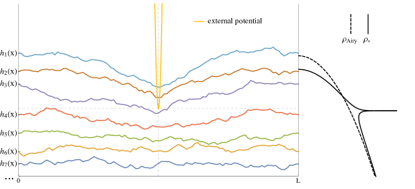
Figure 8: Representation of the seven top Brownian lines subject to the needle external potential. In absence of the potential, the density of the top lines as a function of the depth is described by the edge of the semi-circle $\rho_{\rm Airy}$ (dashed lined on the right) and in presence of a smooth potential, the reorganization of the interfaces imposes a new optimal density $\rho_{*}$ (black line on the right).

The results of the Letter readily apply to describe the linear statistics of the top non-intersecting Brownian interfaces in the ground state in a region of width $N^{-1/6}$ around the top line located at a height $\sim 2\sqrt{N}$. Indeed, if one considers the rescaled heights $\tilde{h}_{i}=(\sqrt{b}h_{i}-2\sqrt{N})4^{1/3}N^{1/6}$, these behave for large $N$ jointly as the Airy_β process $\tilde{h}_{i}\equiv a_{i}$. One observable studied in [14] in the bulk is the center of mass position of the $N_{1}$ top interfaces $H(N_{1})=\frac{1}{N_{1}}\sum_{i=1}^{N_{1}}h_{i}$. As we see, at the edge, in the absence of a potential $W$ it is distributed (up to a scale factor) as the variable $L_{N_{1}}$ in Eq. (44) of the Letter. In presence of the needle potential $W$, parameters can be adjusted so that the soft potential $W$ translate into the soft potential $\phi$ in our units, using the correspondence $W(h_{i}-U)\equiv t\phi(u+t^{-2/3}a_{i})$ with $\sqrt{b}h_{i}\equiv 2\sqrt{N}+4^{-1/3}N^{-1/6}a_{i}$. A practical way to measure the value of $u$ is to measure the position of the center of mass $H(N_{1})$, from which we can determine the optimal density of the first $N_{1}$ brownian lines yielding this specific position. Finally, we represent in Fig. 8 the top interfaces (at a distance of order $N^{-1/6}$ to the first line) subject to an external potential and the optimal density for the first top lines.

23 Appendix: Mellin-Barnes summation

Here we perform the summation of the series which appears in (30). We use a Mellin-Barnes summation method inspired from Lemma 6 of Ref. [30] which was introduced to calculate the sum over replicas in the context of the KPZ equation. For sufficiently nice real test functions $f$, assumed to be positive, the following series admits a closed algebraic form

$$\mathcal{S}(u)=\sum_{n\geq 1}\frac{a^{n}}{n!}(\partial_{u})^{n}f(u)^{n}=\sum_{i}\frac{1}{\mathinner{\!\left\lvert af^{\prime}(u+aw_{i})-1\right\rvert}}-1$$ (301)

where the $\{w_{i}\}$’s are the positive solutions of the equation $f(u+aw)=w$. We use this formula in the Letter only in the case of a unique solution. The present Mellin-Barnes method proposes a formula in the case of multiple solutions. Testing that formula for the present problem is work in progress, we will not use it here.

Proof.

Let us start by manipulating the summand

$$\frac{a^{n}}{n!}(\partial_{u})^{n}f(u)^{n}=\int_{\mathbb{R}}\mathrm{d}y\,\delta(y)\frac{a^{n}}{n!}(\partial_{u})^{n}f(u)^{n+iy}$$ (302)

Let us express the delta in Fourier space and proceed to the change of variable $z=n+iy$,

$$\frac{a^{n}}{n!}(\partial_{u})^{n}f(u)^{n}=\int_{n+i\mathbb{R}}\mathrm{d}z\int_{\mathbb{R}}\frac{\mathrm{d}r}{2i\pi}\,e^{-r(z-n)}\frac{a^{n}}{n!}(\partial_{u})^{n}f(u)^{z}$$ (303)

Let us suppose that we can shift the contour of integration of $z$ such that there is no $n$ dependency anymore. Let us call $\Gamma$ the new shifted contour.

$$\frac{a^{n}}{n!}(\partial_{u})^{n}f(u)^{n}=\int_{\Gamma}\frac{\mathrm{d}z}{2i\pi}\int_{\mathbb{R}}\mathrm{d}r\,e^{-r(z-n)}\frac{a^{n}}{n!}(\partial_{u})^{n}f(u)^{z}$$ (304)

Let us choose the contour $\Gamma=a+i\mathbb{R}$ for some $a\in\,]0,1[$ so that $\Gamma$ is parallel to the imaginary axis and let us proceed to the summation over $n$.

$$\sum_{n\geq 1}\frac{a^{n}}{n!}(\partial_{u})^{n}f(u)^{n}=\int_{\Gamma}\frac{\mathrm{d}z}{2i\pi}\int_{\mathbb{R}}\mathrm{d}r\,e^{-rz}\left(\sum_{n\geq 1}\frac{e^{rn}a^{n}}{n!}(\partial_{u})^{n}\right)f(u)^{z}$$ (305)

One recognizes an exponential series, and more particularly, the series of a translation operator.

$$\begin{split}\sum_{n\geq 1}\frac{a^{n}}{n!}(\partial_{u})^{n}f(u)^{n}&=\int_{\Gamma}\frac{\mathrm{d}z}{2i\pi}\int_{\mathbb{R}}\mathrm{d}r\,e^{-rz}\left[e^{ae^{r}\partial_{u}}-1\right]f(u)^{z}\\ &=\int_{\Gamma}\frac{\mathrm{d}z}{2i\pi}\int_{\mathbb{R}}\mathrm{d}r\,e^{-rz}\left[f(u+ae^{r})^{z}-f(u)^{z}\right]\end{split}$$ (306)

As $\Gamma$ is parallel to the imaginary axis and as both $r$ and $f$ are real valued, one recognizes the integral over $z$ as Fourier transform and we therefore have

$$\begin{split}\sum_{n\geq 1}\frac{a^{n}}{n!}(\partial_{u})^{n}f(u)^{n}&=\int_{\mathbb{R}}\mathrm{d}r\,\left[\delta(\log f(u+ae^{r})-r)-\delta(r)\right]\\ &=\sum_{i}\frac{1}{\mathinner{\!\left\lvert af^{\prime}(u+ae^{r_{i}})-1\right\rvert}}-1\\ \end{split}$$ (307)

where $r_{i}$ are the real solutions of the equation $f(u+ae^{r})=e^{r}$. As $r$ is real, we define $w=e^{r}>0$ which concludes the derivation. ∎

Furthermore suppose now, as in the Letter, that there exists a unique real solution $w=w(u)$ to the equation $f(u+aw)=w$ and that $1-af^{\prime}(u+aw)>0$ for this solution. It is possible to further simplify the series. Indeed, differentiating the equation $f(u+aw)=w$ leads to

$$\left[1-af^{\prime}(u+aw)\right]\mathrm{d}w=f^{\prime}(u+aw)\mathrm{d}u$$ (308)

Inserting this differential relation into Eq. (301) yields

$$\mathcal{S}(u)=\sum_{n\geq 1}\frac{a^{n}}{n!}(\partial_{u})^{n}f(u)^{n}=\frac{af^{\prime}(u+aw)}{1-af^{\prime}(u+aw)}=a\frac{\mathrm{d}w}{\mathrm{d}u}$$ (309)

References