The Properties of the Solar Corona and Its Connection to the Solar Wind

Abstract

The corona is a layer of hot plasma that surrounds the Sun, traces out its complex magnetic field, and ultimately expands into interplanetary space as the supersonic solar wind. Although much has been learned in recent decades from advances in observations, theory, and computer simulations, we still have not identified definitively the physical processes that heat the corona and accelerate the solar wind. In this review, we summarize these recent advances and speculate about what else is required to finally understand the fundamental physics of this complex system. Specifically:

• We discuss recent sub-arcsecond observations of the corona, some of
  which appear to provide evidence for tangled and braided magnetic
  fields, and some of which do not.

• We review results from three-dimensional numerical simulations that,
  despite limitations in dynamic range, reliably contain sufficient heating
  to produce and maintain the corona.

• We provide a new tabulation of scaling relations for a number of
  proposed coronal heating theories that involve waves, turbulence,
  braiding, nanoflares, and helicity conservation.

An understanding of these processes is important not only for improving our ability to forecast hazardous space-weather events, but also for establishing a baseline of knowledge about a well-resolved star that is relevant to other astrophysical systems.

1 INTRODUCTION

The solar corona is the hot and ionized outer atmosphere of the Sun. Much of the corona’s plasma is confined by the solar magnetic field in the form of closed loops and twisted arcade-like structures. In addition, some coronal plasma expands into interplanetary space as a supersonic outflow known as the solar wind. Figure 1 shows two different views of the corona and its collection of closed and open magnetic fields. Despite almost a century of study, the physical processes responsible for heating the corona and accelerating the solar wind are not yet understood at a fundamental level. However, an incredible amount has been learned about this complex system from continuous advances in observations, theory, and numerical simulations. The corona and solar wind have been put to use as laboratories for studying a wide range of processes in plasma physics and magnetohydrodynamics (MHD), and they provide access to regimes of parameter space that are often inaccessible to Earth-based laboratories.[] MHDmagnetohydrodynamics

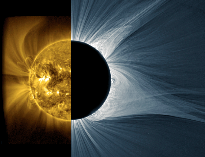
Figure 1: Complementary views of the solar corona. Left: Extreme-ultraviolet emission image from the SWAP (Sun Watcher using Active-pixel-system detector and image Processing) telescope on the PROBA2 spacecraft (Seaton et al., 2013). The image was taken in the 17.1 nm wavelength band on 2014 July 25. Right: Visible-band scattered light from the total solar eclipse of 2017 August 21, adapted from original images obtained and processed by M.  Druckmüller, P.  Aniol, and S.  Habbal (see also Druckmüller et al., 2006).

The ever-changing corona and solar wind can substantially affect the near-Earth space environment. For example, the ultraviolet (UV) and X-ray radiative output of the corona fluctuates by several orders of magnitude—on timescales between minutes and decades—and this drives large changes in the ionosphere. When dynamic variability in the solar wind impacts the Earth’s magnetosphere, it can interrupt communications, damage satellites, disrupt power grids, and threaten the safety of humans in space. There is an ever-increasing need to understand how this so-called space-weather activity affects human society and technology, and to produce more accurate forecasts (see, e.g., Koskinen et al., 2017). Such practical advances are made possible only when there is concurrent research devoted to answering more fundamental questions such as “what heats the corona?” and “what determines the solar wind speed for a given magnetic-field configuration?”

This paper reviews our current understanding of the solar corona and its connection to the solar wind. We attempt to provide: (1) a broad reconnaissance of the present state of the field, (2) a selection of useful pointers into the primary research literature, and (3) a brief and selective overview of our shared history. Because one paper cannot exhaustively cover all work done in such a large field, we also urge readers to fill in the gaps with other reviews. Useful surveys of contemporary ideas about the solar corona have been presented by Billings (1966), Withbroe & Noyes (1977), Kuperus et al. (1981), Narain & Ulmschneider (1990), Low (1996), Aschwanden (2006), Klimchuk (2006), Golub & Pasachoff (2010), Parnell & De Moortel (2012), Reale (2014), Schmelz & Winebarger (2015), Velli et al. (2015), and Hara (2018). General summaries of the problems and controversies regarding the solar wind have been presented by Parker (1963), Dessler (1967), Holzer & Axford (1970), Hundhausen (1972), Leer et al. (1982), Axford et al. (1999), Meyer-Vernet (2007), Zurbuchen (2007), Bruno & Carbone (2013), Abbo et al. (2016), and Cranmer et al. (2017). We leave the study of the most explosive events—e.g., solar flares and coronal mass ejections (CMEs)—to other reviews (see, e.g., Fletcher et al., 2011; Gopalswamy, 2016).[] CMEcoronal mass ejection

2 BRIEF HISTORY

2.1 The Million-Degree Corona

Although descriptions of an ethereal glow surrounding the eclipsed Sun can be found going back to antiquity, the first usage of the actual word corona (meaning a wreath, garland, or crown) for this phenomenon was probably by Giovanni Cassini. On the occasion of the May 1706 solar eclipse, Cassini referred to “une couronne d’une lumière pâle,” or a crown of pale light (Westfall & Sheehan, 2015). Significant progress in understanding the Sun’s tenuous outer atmosphere began to accumulate with the development of spectroscopy in the latter half of the 19th century. In 1868, Janssen and Lockyer discovered evidence for a new chemical element (helium) at the solar limb in the form of a bright 587.6 nm emission line. Just one year later, during the solar eclipse of August 1869, Harkness and Young first observed another emission line, at 530.3 nm, that did not correspond to any known element. Lockyer (1869), in the first issue of Nature, discussed the ways this observation was “…bizarre and puzzling to the last degree!” Speculation that this line implied the existence of another new element (“coronium”) persisted for decades, and in that time a few dozen other mysterious coronal lines were found.

Eventually, Grotrian (1939) and Edlén (1943) utilized insights from the new theory of quantum mechanics to determine that the coronal emission lines were associated with unusually high ionization states of iron, calcium, and nickel. This is often assumed to be the primary evidence for a hot corona, but Alfvén (1941) assembled several other pieces of observational evidence that all point in this direction. For example, the white-light continuum spectrum of the low corona is dominated by Thomson scattering between photospheric photons and free electrons. Thus, the radial variation of the white-light intensity is a probe of the radial variation of electron density. Alfvén (1941) found that the measurements of Baumbach (1937) would be consistent with hydrostatic equilibrium only for electron temperatures of about $10^{6}$ K. In addition, the lack of sharp Fraunhofer absorption lines in the coronal white-light spectrum pointed to the existence of substantial Doppler broadening due to random thermal motions of the electrons, which also requires similar million-degree temperatures (see also Grotrian, 1931; Reginald et al., 2017). Alfvén (1941) also made the earliest estimate of the energy flux required to heat the corona, and his computed value of 0.2 kW m^-2 is consistent with modern calculations (see Section 5.1).

The corona emits most of its radiation in the ultraviolet and X-ray parts of the spectrum, but these wavelengths are absorbed strongly by the Earth’s atmosphere. In the early 1940s, the extent of this atmospheric absorption was not known, and this pushed experimenters—along with spectrometers sensitive to UV radiation—to mountain peaks in order to attempt to extend the solar spectrum into the ultraviolet. In 1946, a team of researchers launched an ultraviolet spectrometer on a V-2 rocket for the first time, resulting in both extending the Sun’s ultraviolet spectrum to lower wavelengths and opening a door to space-based observations that are now the cornerstone of our knowledge of the solar corona (Tousey, 1967). The initial rocket flights focused on capturing the solar spectrum to determine the elemental makeup of the solar corona. The data were compared to spectra obtained from ground-based laboratories and theoretical calculations to identify the emitting elements and ions. Data taken from different rocket flights were compared to understand the variability of the Sun. Additionally, spectroheliograms (also called overlapograms, i.e., spectrally dispersed images of the Sun on which spatial and spectral information are overlapping) were made with slitless spectrometers. These images, typically made along with well-isolated, strong, cool spectral lines to aid in interpretation, complemented ground-based observations.

In the 1960s, a pinhole camera was launched on a rocket, and it obtained the first X-ray photograph of the Sun that provided the first glimpse of the structure of the million-degree corona (Blake et al., 1963). This photo revealed that the high-temperature plasma is not evenly distributed throughout the solar atmosphere, but is instead confined to localized “X-ray plages,” now commonly called active regions. These short-duration rocket flights drove the desire for continuous solar observations above the Earth’s atmosphere. Subsequently, NASA launched several Orbiting Solar Observatories (OSO–1 through OSO–8) from 1962 to 1975, which had autonomous UV, extreme ultraviolet (EUV), and X-ray instruments on board.[] EUVextreme ultraviolet: wavelengths of 10–100 nm The first space station, Skylab, in operation from 1973 to 1979, also served as a solar observatory, allowing the astronauts to operate some of the instruments manually. These early experiments and their discoveries led to modern-day observatories on satellites, such as the Japanese-led Yohkoh (1991–2001) and Hinode (2006–present), and the NASA-led Solar and Heliospheric Observatory (SOHO; 1996–present), Solar Terrestrial Relations Observatory (STEREO; 2006–present), and Solar Dynamics Observatory (SDO; 2010–present), as well as several smaller class missions. Over time, the instruments on these observatories have improved the spatial or spectral resolution, wavelength coverage, cadence or data volume, or had non-traditional orbits. There also continues to be a rich sounding rocket and balloon program that serves as a testbed for new instruments and technologies.

Both historical and modern-day data comprise a broad range of diagnostics that yield a great deal of information about the solar corona. Spectroscopic data in UV, EUV, and X-ray wavelengths provide information on the distribution of emission as a function of temperature, density, and velocity, and on the composition of the coronal plasma (see review by Del Zanna & Mason, 2018). Images of the Sun in broad X-ray passbands or narrow EUV passbands, facilitated by the development of multilayer coatings, provide the spatial distribution of the emission and also a rough estimate of the emission measure distribution as a function of the temperature of the plasma. These observations have been compared to photospheric magnetic field measurements, which are commonly obtained from both ground-based and space-based observatories. One of the most important realizations from this collective data set is that the X-ray luminosity of active regions is proportional to the total unsigned photospheric magnetic flux (Fisher et al., 1998). This observation was expanded over 12 orders of magnitude by including quiet Sun regions, active regions, and stellar coronae (Pevtsov et al., 2003). These relatively simple observations imply that the magnetic field plays an important role in the heating of the corona.

Early spectroscopic observations revealed that the composition of the corona did not always match the composition of the underlying photosphere. Instead, the abundances of a few elements sometimes appeared to be enhanced, while the abundances of other elements remained closer to their photospheric values. The enhanced elements, such as iron and silicon, have low values of their first ionization potential (FIP), while the non-enhanced elements, such as oxygen and neon, have high FIP.[] FIPfirst ionization potential The so-called “FIP bias,” i.e., the corona-to-photosphere enhancement ratio of elements with FIP lower than about 10 eV, is generally found to be about 2–4, and it depends strongly on the coronal structure (see reviews by Meyer, 1985; Feldman, 1992; Sylwester et al., 2010). The fractionation process that creates the FIP effect is likely closely related to the mechanism that heats the corona (Laming, 2015).

Combining spatially resolved data with spectroscopy can provide information on individual closed coronal structures, the so-called coronal loops (see Reale, 2014). When observed in X-rays, the loops were initially found to be long-lived and to have densities and temperatures consistent with steady, uniform heating (e.g., Porter & Klimchuk, 1995). However, this result was challenged by observations made at EUV wavelengths (Klimchuk et al., 2010). The densities of the loops are as much as three orders of magnitude larger than predicted by steady heating (e.g., Winebarger et al., 2003a), and the observed pressure stratification does not agree with the expected gravitational scale height (e.g., Aschwanden et al., 2001). In addition, the temperatures along the loops are more uniform than predicted by steady heating (Lenz et al., 1999). Though the loops appear to be relatively cool (Viall & Klimchuk, 2012), the loops’ lifetimes are longer than expected for models of radiative and conductive cooling (Winebarger et al., 2003b). Finally, many loops exhibit bulk flows (e.g., Winebarger et al., 2002) and values of the nonthermal velocity (e.g., Brooks & Warren, 2016) that do not appear to match what is expected for several simple models of uniform heating. We discuss some of the physical processes underlying these phenomena in Section 5.5.

2.2 The Supersonic Solar Wind

Starting in the late 19th century, there arose speculation about a direct connection between phenomena occurring on the Sun and specific kinds of events taking place on Earth. Carrington (1859) and others took note of the fact that the solar flare observed in September 1859 was soon followed by strong geomagnetic storms (i.e., fluctuations in the Earth’s magnetic field) and bursts of electric current along telegraph lines. Birkeland (1908), reporting on many years worth of data collected on polar expeditions, made a case that both geomagnetic storms and intense auroral activity “…should be regarded as manifestations of an unknown cosmic agent of solar origin.” It took several more decades to narrow down the precise physical nature of this chain of cause and effect. Chapman (1918) suggested that the Sun ejects sporadic clouds or beams of charged particles into otherwise empty space, and Hulburt (1937) focused more on ultraviolet radiation as an excitation mechanism for geomagnetic storms and the aurora. Biermann (1951) concluded from the observed properties of comet ion tails that the solar system appears to be filled with charged particles (i.e., “corpuscular radiation”) that are always flowing out radially from the Sun.

Parker (1958) juxtaposed Biermann’s idea of a continuous outflow of solar particles with the earlier discovery of the high-temperature corona, and he concluded that these two concepts are inextricably connected. The high gas-pressure gradient in a hot corona produces an outward force that counteracts gravity and allows for a time-steady accelerating flow of plasma away from the Sun. Parker coined the term solar wind for this flow, which starts out slow and subsonic near the solar surface and becomes fast and supersonic at larger heliocentric distances. The transition between subsonic and supersonic regimes occurs at a so-called critical point. Initially, the Parker (1958) wind solution was criticized for being too finely tuned; i.e., it seemed unlikely that the system would naturally choose this one critical solution out of an essentially infinite number of others that do not become supersonic (see, e.g., Chamberlain, 1961). Although observations soon settled the matter in Parker’s favor, it has also been determined that the critical solution is essentially a stable attractor of this dynamical system, and that all of the other possible outflow solutions are unstable (Velli, 1994).

As noted above, the community had to wait only a few years until the first in situ measurements of particles and fields beyond the Earth’s magnetosphere. Hundhausen (1972), Neugebauer (1997), and many others have told the story of the discovery of the continuous and supersonic solar wind at the dawn of the Space Age. In the first few years of interplanetary exploration, it was revealed that the solar wind often undergoes transitions between a dense and slow state (i.e., speeds of 250–450 km s^-1) and a tenuous and fast state (500–800 km s^-1). Also, the radial magnetic field frequently alternates sign to form “magnetic sectors” that recur with the Sun’s 27-day rotation. These largest-scale plasma structures in the solar wind are now generally believed to be connected to the topology and geometry of the Sun’s complex magnetic field (see Section 6.2). There is also considerable variability on smaller scales, such as stochastic MHD turbulence (Coleman, 1968) and coherent Alfvén waves (Belcher & Davis, 1971). The first few decades of solar wind exploration saw missions that explored inside the orbit of Mercury (Helios; Schwenn & Marsch 1991), far past Pluto (Voyager; Burlaga et al.  1996), and out of the ecliptic plane altogether (Ulysses; Marsden 2001).

3 ADVANCES IN REMOTE-SENSING OBSERVATIONS

With the plethora of ever-improving observations of the corona available to solar physicists after the advent of rocket- and satellite-borne observatories, one might wonder why the solar corona heating problem is still a problem. The answer of course is that many coronal heating theories, discussed in detail in Section 5, predict very similar observational consequences in the regimes where observations are easiest to make. This often makes it difficult to use data from current observatories to discriminate between the different heating theories (see, for instance, Winebarger & Warren, 2004). Here we provide some recent observations that push the boundaries of current instrumentation. Not surprisingly, many of these observations originate in suborbital instruments.

Nearly all coronal heating theories predict that heating will happen sporadically on spatial scales much smaller than resolved by current instrumentation, meaning that coronal structures or loops that are resolved by current instrumentation are actually formed of many sub-resolution strands, each tracing a magnetic field line. Some theories require that the magnetic strands be twisted or braided, but normally the resolved coronal structures, such as those shown in Figure 1, do not show significant evidence for twisting or braiding on large scales. Unfortunately, it is unclear whether the strands become more tangled when observed in higher resolution. In 2012, the High-Resolution Coronal Imager (Hi-C) sounding rocket was launched, and it obtained the highest spatial resolution (0.2–0.3^′′) images of the solar corona in a narrow EUV wavelength channel. This data set, for the first time, resolved two examples of coronal braiding in an active region core by direct observation of the high-temperature plasma (Cirtain et al., 2013). Another way of inferring the coronal field structure is by observing chromospheric plasma at coronal heights in the form of “coronal rain,” cool dense plasma that forms high in the solar atmosphere and slides down the magnetic field lines. Coronal rain is thought to be caused by strong, steady heating near the footpoints of the loops, which gives rise to thermal nonequilibrium conditions near the loop apex (e.g., Müller et al., 2005). Using the Crisp Imaging Spectro-Polarimeter (CRISP) instrument at the Swedish Solar Telescope, coronal rain was observed in the H I Balmer $\alpha$ line at the diffraction limit of 0.14^′′ (Antolin & Rouppe van der Voort, 2012). No evidence of coronal braiding was found as the rain traced the magnetic field strands as it fell. Figure 2 illustrates these apparently conflicting results.

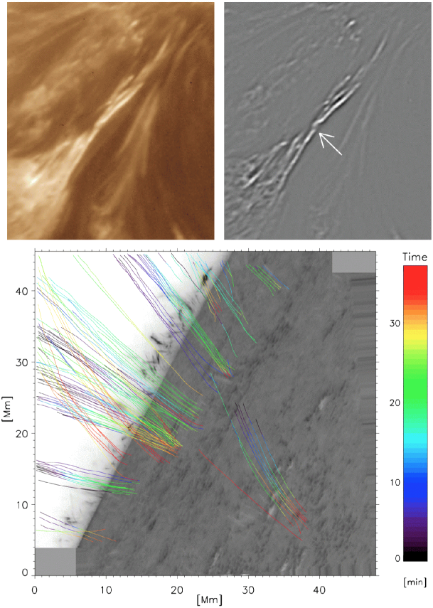
Figure 2: Recent observations find conflicting results about the degree of magnetic tangling of coronal field lines at scales of order 0.2^′′. Top left: Braided active region structure imaged by Hi-C at a wavelength of 19.3 nm, on 2012 July 11. Top right: Enhanced version of the Hi-C image made with an unsharp-masking technique (see Cirtain et al., 2013); an arrow highlights a braided structure. Shortly after this image was acquired, a heating event was observed at this location implying that energy stored in the magnetic field was released. Bottom: The paths of coronal-rain plasma parcels, observed by CRISP on 2009 May 10, suggest that the field is smooth and unbraided (Antolin & Rouppe van der Voort, 2012).

Different coronal heating theories predict different frequencies of heating on the proposed sub-resolution strands. Correspondingly, changes in the heating frequency imply different relative amounts of high-temperature ($T>3$ MK) emission, and this further suggests that high-temperature plasma could be a key discriminator in coronal heating. Unfortunately, high-temperature plasma—which also tends to have low emission measure—is particularly difficult to detect with current satellite instrumentation that is most sensitive to the brighter 1–3 MK plasma (Winebarger et al., 2012). The Extreme Ultraviolet Normal Incidence Spectrograph (EUNIS–13) sounding rocket instrument was successful in determining that the Fe XIX line (which has a peak formation temperature of 8.9 MK) was pervasive and weak through an active region. This provided strong evidence that the heating in the active region was infrequent, potentially from small-scale magnetic reconnection events called nanoflares. The Focusing Optics X-ray Solar Imager (FOXSI–2) sounding rocket flight also detected signatures of hot plasma in two localized regions in a solar active region, indicating the possibility of low-frequency nanoflare heating (Ishikawa et al., 2017). However, significant evidence also exists to indicate high-frequency heating, such as expected for wave dissipation models. The formation of the above-mentioned coronal rain relies on near-steady and highly stratified heating. Such energy deposition would not only drive coronal rain, but would also cause high-temperature structures to disappear and reappear on long time scales; such behavior has recently been detected (Froment et al., 2017).

Another indirect observation in support of magnetic reconnection is the impact of nonthermal particles as they spiral down magnetic field lines and interact with the denser plasma near the magnetic footpoints. Testa et al. (2014) discovered evidence for nonthermal particles in a highly localized region in data from the Interface Region Imaging Spectrograph (IRIS), which provides high spatial resolution and high cadence data of the chromosphere and transition region. These observations indicate that there may indeed be signatures of magnetic reconnection in observations of improved temporal and spatial resolutions. The presence of nonthermal particles can also be inferred from radio noise storms (James & Subramanian, 2018).

4 ADVANCES IN IN-SITU MEASUREMENTS

Recent decades have seen vast improvements in the sensitivity, accuracy, and cadence of instruments that measure the properties of particles and electromagnetic fields in space. These measurements have verified that the solar wind is a natural continuation of the highly structured, dynamic, and nonequilibrium corona. The multiple particle populations in the ionized solar wind (e.g., protons, helium nuclei, free electrons, and heavy ions) undergo infrequent collisions with one another, and thus they tend not to be in a common state of thermal equilibrium. The particles often exhibit distinctly different bulk flow speeds, temperatures, and velocity distribution anisotropies, and these differences are most pronounced in the lowest-density regions with the fewest interparticle collisions (Marsch, 2006; Kasper et al., 2008; Cranmer et al., 2017). These differences—usually quantified as a function of the charge and mass of each type of particle—are also useful diagnostics of the physical processes responsible for heating the plasma.

Precise measurements of heavy-ion abundances and ionization states are known to carry information about the physical processes that affected the ions back in the corona. These composition signatures are “frozen in” near the solar surface and they remain invariant over much of the wind’s journey into interplanetary space (e.g., Zurbuchen, 2007). Above a certain point in the low corona, the ions collide with virtually no more electrons, so they do not undergo any further ionization or recombination. These features are often used to trace wind streams down to specific coronal magnetic structures, and their ionization states are indirect measures of the corona’s electron temperature. In addition, some types of slow solar wind are seen to contain subtle enhancements in the abundances of low-FIP elements, which is similar to the behavior of some coronal loops (see Section 2.1). The explanation for why the observed distribution of abundances in the corona and solar wind departs from the photospheric distribution is still not yet known (see, however, Laming, 2015; Reames, 2018), and measurements continue to be refined in order to tighten constraints on the proposed theories.

The heliospheric measurement of MHD turbulence has also become more sophisticated in the last few decades. Combining particle and field data from multiple instruments has led to at least 9 orders of magnitude of coverage in temporal and spatial scales (Bruno & Carbone, 2013; Kiyani et al., 2015). In the solar wind, there is continuous activity across frequencies between $10^{-6}$ and $10^{+3}$ Hz. This corresponds to spatial eddies flying past the spacecraft with sizes from several astronomical units (AU) down to a fraction of a kilometer. The smallest sizes overlap with the proton and electron gyroradii and inertial lengths, and kinetic departures from ideal MHD are consistently seen at those scales. These departures include unequal temperatures for electrons, protons, and heavier ions, differential flows between these species, and non-Maxwellian velocity distributions. The nature of the plasma fluctuations is also being revealed by the use of formation-flying groups of spacecraft. When these instruments pass through the same parcel of turbulent plasma at slightly different times and locations, the signals can be combined to disambiguate the spatial from the temporal fluctuations; see, e.g., studies from Cluster (Goldstein et al., 2015) and the Magnetospheric Multiscale Mission (Bandyopadhyay et al., 2018). This kind of high-resolution data continues to be analyzed with a wide range of statistical techniques that probe the intermittency, anisotropy, and multifractality of solar wind turbulence. For space plasmas in both the MHD and kinetic physical regimes, turbulence appears to be fundamentally more complex than the traditional isotropic turbulence found in incompressible hydrodynamics (see, e.g., Matthaeus & Velli, 2011).

5 CORONAL HEATING PHYSICS

Although the precise mechanisms heating the corona and solar wind are not yet understood, the ultimate energy source is generally understood to be the Sun’s roiling convection zone. The following subsections follow the flow of energy from below the photosphere up through the extended corona, and they summarize as many of the proposed heating processes as possible. It should be noted, however, that the ultimate solution of the coronal heating problem may not involve one single process that acts in isolation. The solar corona/wind system is sufficiently complex that it is likely that different combinations of multiple processes are heating the plasma in different regions and at different times.

5.1 The Overall Flow of Energy

In the convection zone, thermal energy is transported up by the rising of hot parcels of gas and the falling of cooler parcels. Approaching the solar surface, convection carries nearly all of the energy that is ultimately released as radiation, so the energy flux is given by $F_{\odot}\approx\sigma T_{\rm eff}^{4}$, where $\sigma$ is the Stefan-Boltzmann constant and $T_{\rm eff}=5770$ K is the effective temperature. In the strongly unstable regions of the subsurface convection zone, $F_{\odot}\approx 63000$ kW m^-2. However, the photosphere tends to sit several scale heights above the top of the unstable region, and most of that flux escapes as radiation. We observe granulation upflows and downflows in the photosphere, but the residual kinetic energy flux (i.e., $\rho u^{3}/2$, where $\rho$ is the mass density and $u$ is the bulk flow speed) is only of order 500 kW m^-2. This is the source of mechanical energy that is often assumed to be the available pool for energizing the upper atmosphere. Of course, this estimate does not distinguish between energy carried upward by rising granules, that carried downward in the intergranular lanes, and the energy in horizontal motions.

In addition, in many theories of coronal heating there is only a small filling factor $f$ of the photospheric surface that is connected magnetically to the corona. In that case, the energy available at a point in the corona is diluted by multiplying the mean photospheric flux by $f$. The filling factor is essentially the coronal magnetic flux density divided by the field strength in the small photospheric sources, which tends to be about 1500 G, or close to the equipartition field strength (i.e., the field strength at which magnetic pressure balances gas pressure). To within an order of magnitude, active regions tend to exhibit $f\approx 0.1$ and weaker-field regions such as the quiet Sun and coronal holes tend to exhibit $f\approx 0.01$. Thus, the available energy flux into those regions is probably about 50 and 5 kW m^-2, respectively. Withbroe & Noyes (1977) estimated the magnitudes of energy flux required for coronal heating in active regions, coronal holes, and the quiet Sun to be about 10, 0.8, and 0.3 kW m^-2, respectively, and this is consistent with the available diluted fluxes.

The process of coronal heating involves both the large-scale transport of energy from lower to upper layers and the irreversible conversion of mechanical kinetic energy into random thermal motions of the particles. Intermediate steps—such as the excitation of propagating waves or temporary storage in non-potential magnetic fields—are often necessary. The ultimate conversion to thermal energy tends to be most efficient when the energy is transferred from large-scale, long-lived structures to small-scale, bursty, and short-lived structures. Such a transfer is often triggered by some kind of nonlinearity or instability in the system, and the rate of heating becomes highly intermittent. It often makes more sense to refer to the local volumetric heating rate $Q$ (i.e., the power delivered per unit volume) rather than the upward vector energy flux ${\bf F}$. The heating rate $Q$ is formally defined as as $|\nabla\cdot{\bf F}|$, but it can be expressed approximately as $|{\bf F}|/L$, the energy flux distributed over a coronal loop of length $L$.

5.2 Acoustic Waves and the Chromosphere

Convective upflows and downflows are known to give rise to both stochastic “noise” and to globally resonant pressure-mode oscillations (see, e.g., Schwarzschild, 1948; Narain & Ulmschneider, 1990; Stein et al., 2004). Some fraction of this acoustic wave energy propagates up from the photosphere to the chromosphere, and the longitudinal velocity amplitude $v_{\parallel}$ generally increases with increasing height in order to conserve energy flux. For motions that survive to the point where the amplitude becomes of the same order of magnitude as the sound speed $c_{s}$, an initially sinusoidal wavetrain will evolve into a sawtooth-like collection of thin shocks. This is believed to occur no more than 0.5–1 Mm above the photosphere, and at these heights the plasma $\beta$ (i.e., the ratio of gas pressure to magnetic pressure) is either much larger than or of order unity. Therefore, much of the subsequent dissipation and heating due to these fluctuations is often treated in the hydrodynamic (zero magnetic field) limit.

In general, acoustic waves can be dissipated by collisional transport effects (e.g., heat conduction, viscosity, or resistivity), radiative losses, entropy gain at shock discontinuities, or kinetic wave-particle interactions. A representative scaling for the volumetric heating rate can be given as

$$Q\,\approx\,{\cal E}\,\rho v_{\parallel}^{2}c_{s}/\lambda_{\parallel}\,\,\,,$$ (1)

where ${\cal E}$ is a dimensionless efficiency factor and $\lambda_{\parallel}$ is the wavelength. Cranmer et al. (2007) discussed the limiting cases of dissipation due to weak ($v_{\parallel}\ll c_{s}$) and strong ($v_{\parallel}\gg c_{s}$) shocks, and found ${\cal E}\approx 1.8v_{\parallel}/c_{s}$ in the weak limit and ${\cal E}\approx 0.4$ in the strong limit. In most numerical models, the development of shocks and their rapid dissipation usually means that $v_{\parallel}$ never becomes larger than about $c_{s}$ itself. In the upper chromosphere and low corona, heat conduction also becomes a significant source of dissipation, whether the fluctuations are sinusoidal or shock-like. For this process, ${\cal E}\approx Pe^{-1}$, where $Pe$ is the Péclet number, or the ratio of $c_{s}\lambda_{\parallel}$ to the conductive diffusion coefficient.

In the weakly magnetized internetwork regions of the Sun (i.e., supergranular cell centers), there is still no agreement about whether the dissipation of acoustic fluctuations is strong enough on its own to heat the chromosphere. Existing observations have sometimes pointed to an affirmative answer (Cuntz et al., 2007; Bello González et al., 2010) and sometimes to a negative answer (Carlsson et al., 2007; Beck et al., 2012). Numerical simulations are able to reproduce much of the observed structure and time-dependent dynamics in the non-magnetic chromosphere (e.g., Carlsson & Stein, 1997). However, many simulations tend to produce a highly intermittent state; i.e., hot shocks surrounded by larger regions that may be too dark and cool to produce the steady emission seen in many chromospheric spectral lines (Kalkofen, 2012). No matter the role of acoustic waves/shocks in the chromospheric energy budget, it is clear that their dissipation tends not to leave much power available at larger heights to heat the corona (Athay & White, 1978; Cranmer et al., 2007). Thus, in recent years the focus has shifted heavily to magnetic fields and MHD fluctuations as a primary heating mechanism for both the chromosphere (Jess et al., 2015) and corona (Section 5.3).

5.3 A Plethora of Proposed MHD Processes

Most of the magnetic field lines that are anchored in the photospheric granulation ($\beta>1$) are also connected to the low-density corona ($\beta<1$), and the complex interplay between these two disparate regions is far from understood. When considering the transport of magnetic energy up from the surface, the Poynting flux ${\bf S}$ helps to specify how much is available. The injection of energy via the Poynting flux must be balanced either by dissipation (i.e., heating) or by a long-term buildup of magnetic energy in the system. In ideal MHD, with a vector magnetic field ${\bf B}$ and fluid velocity ${\bf v}$, the Poynting flux is given by ${\bf S}={\bf B}\times({\bf v}\times{\bf B})/4\pi$. Considering the solar surface as a flat plane, the vertical component is

$$S_{z}\,=\,\frac{1}{4\pi}\left[v_{z}B_{\perp}^{2}-({\bf v}_{\perp}\cdot{\bf B}_{\perp})B_{z}\right]\,\,,$$ (2)

where $z$ and $\perp$ denote the vertical and horizontal components, respectively (see Welsch, 2015). Although the horizontal component of ${\bf S}$ is sometimes considered as a source of coronal shear (Knizhnik et al., 2018), it is mostly the vertical component that is believed to supply energy to the corona. In Equation 2, the first term in square brackets corresponds to flux emergence from below the surface (Fisk et al., 1999; Cheung & Isobe, 2014). The second term corresponds to horizontal jostling of an arbitrarily inclined field line that passes through the surface. In regions where new flux is not emerging, the jostling term provides an energy flux that scales as $S_{z}\approx\rho V_{\rm A}^{2}v_{\perp}$, where $V_{\rm A}=B/\sqrt{4\pi\rho}$ is the Alfvén speed. Typical properties of the photospheric granulation ($v_{\perp}=1$ km s^-1) and the coronal magnetic field ($B=50$ G) thus appear to be able to supply energy fluxes of order 20 kW m^-2.

In the remainder of this subsection we summarize many of the mechanisms that have been proposed for dissipating the available Poynting flux as heat. Historically, there have been two major schools of thought that depend on the relative values of two important timescales. First, the so-called Alfvén travel-time $\tau_{\rm A}$ describes how long it takes a linear perturbation to traverse a significant distance along the coronal magnetic field. One can write $\tau_{\rm A}=L/V_{\rm A}$, where $L$ is either the loop length (for closed magnetic fields) or a representative solar-wind scale height (for open fields). Second, the photospheric driving timescale $\tau_{\rm ph}$ is a characteristic time over which the granular motions can make major changes in the field at the footpoints. This quantity is often written as $\tau_{\rm ph}=\lambda_{\perp}/v_{\perp}$, where $\lambda_{\perp}$ is a horizontal correlation length for footpoint driving.

Given the above definitions, we can parameterize the MHD coronal heating rate $Q$ in terms of the vertical Poynting flux, spread out over the macroscopic scale length $L$, multiplied by a still-undetermined efficiency factor,

$$Q\,\approx\,{\cal E}\,\rho V_{\rm A}^{2}v_{\perp}/L\,\,\,.$$ (3)

Table 1 provides a sampling of proposals for how the efficiency factor ${\cal E}$ depends on dimensionless ratios such as

$$\Lambda\,=\,\lambda_{\perp}/L\,\,\,,\,\,\,\,\,\,\,\Theta\,=\,\tau_{\rm A}/\tau_{\rm ph}\,\,\,.$$ (4)

For simplicity’s sake, dimensionless numerical factors of order unity are not included in Table 1, and the expressions themselves tend to be time averages. The traditional limit of slowly evolving quasi-static equilibria (i.e., direct-current, or DC theories) corresponds to $\Theta\ll 1$, and the limit of rapid footpoint-driving that produces waves and other propagating fluctuations (i.e., alternating-current, or AC theories) corresponds to $\Theta\gg 1$.[] ACalternating current,
$\tau_{\rm A}\gg\tau_{\rm ph}$ DCdirect current,
$\tau_{\rm A}\ll\tau_{\rm ph}$

Table 1: MHD coronal heating theories: Efficiency scalings relative to the Poynting flux

Model description	Efficiency ($\cal E$)	Example reference
Wave Dissipation (AC) Models
Alfvén-wave collisional damping	$\Lambda^{1}\Theta^{2}Re^{-1}$	Osterbrock (1961)
Resonant absorption	$\Lambda^{1}\Theta^{1}$	Ruderman et al. (1997)
Phase mixing	$\Lambda^{1}\Theta^{4/3}Re^{-1/3}$	Roberts (2000)
Surface-wave damping	$\Lambda^{1/2}\Theta^{3/2}(\Sigma/Re)^{1/2}$	Hollweg (1985)
Fast-mode shock train	$\Lambda^{2}\Theta^{3}$	Hollweg (1985)
Switch-on MHD shock train	$\Lambda^{3}\Theta^{4}$	Hollweg (1985)
Turbulence Models
Kolmogorov-Obukhov cascade	$\Lambda^{1}\Theta^{2}$	Hollweg (1986)
Iroshnikov-Kraichnan cascade	$\Lambda^{2}\Theta^{3}$	Chae et al. (2002)
Hybrid triple-correlation cascade	$\Lambda^{1}\Theta^{3}(1+\Theta)^{-1}$	Zhou & Matthaeus (1990)
Reflection-driven cascade	$\Lambda^{1}\Theta^{2}(f_{+}^{2}f_{-}+f_{-}^{2}f_{+})$	Hossain et al. (1995)
2D boundary-driven cascade	$\Lambda^{2/3}\Theta^{1/3}$	Heyvaerts & Priest (1992)
Line-tied reduced MHD cascade	$\Lambda^{1}\Theta^{1/2}$	Dmitruk & Gómez (1999)
Footpoint Stressing (DC) Models
Current-layer random walk	$\Lambda^{1}$	Sturrock & Uchida (1981)
Current-layer shearing	$\Lambda^{1}(1+\Theta^{2})^{1/2}(1+\Lambda^{2})^{-1/2}$	Galsgaard & Nordlund (1996)
Braided discontinuities	$\Lambda^{2}\Theta^{1}$	Parker (1983)
Flux cancellation	$\Lambda^{1}\Theta^{1}(\phi^{8/3}-\phi^{4/3})$	Priest et al. (2018)
Taylor Relaxation Models
Tearing-mode reconnection	$\Lambda^{1}\Theta^{1}(1-\alpha L)^{-5/2}$	Browning & Priest (1986)
Hyperdiffusive reconnection	$\Lambda^{1}\Theta^{-1}(\alpha L)^{2}$	van Ballegooijen & Cranmer (2008)
Non-ideal/slipping reconnection	$\Theta^{-1}(\alpha L)^{1}$	Yang et al. (2018)

The following subsections describe four classes of proposed models in more detail, but it is worthwhile to first give representative values for some of the parameters. For photospheric granulation, $\lambda_{\perp}$ probably ranges between 0.1 and 1 Mm, and for typical coronal loops, $L\approx 5$–500 Mm. Thus, nearly all coronal regions tend to exhibit $\Lambda\ll 1$. Values for the timescales are more dependent on context. A typical granule lifetime of 5–10 minutes may be used for $\tau_{\rm ph}$, but small internal motions inside intergranular flux tubes may remain coherent for 1 minute or less (van Ballegooijen et al., 2011). The Alfvén travel-time $\tau_{\rm A}$ may be as small as 10 seconds if only the coronal part of the loop is considered, but it may be longer than 10 minutes if one also counts the travel-time through both chromospheres at the footpoints (van Ballegooijen et al., 2014). In some theories, the fundamental driving quantity is $v_{\perp}$, and this varies by more than an order of magnitude depending on whether it is evaluated at the photosphere ($\sim$1 km s^-1) or in the upper chromosphere (20–40 km s^-1).

5.3.1 Wave Dissipation (AC) Models

Waves are often proposed as an agent for coronal heating because they provide a way for energy to be generated at the photosphere and then be transmitted (with minimal losses) up to the corona, where the conversion to heat can then occur. The MHD Alfvén wave is the least-damped oscillation mode in the chromosphere, and it is observed ubiquitously in the solar atmosphere (e.g., Tomczyk et al., 2007; Jess et al., 2015). However, there are ongoing debates about whether a more specialized nomenclature should be used to distinguish between different types of transverse and incompressible waves (Mathioudakis et al., 2013). In any case, for this overall class of wave modes, the jostling term in the Poynting flux can be expressed generally as $S_{z}\approx\rho v_{\perp}^{2}V_{\rm A}$, which implies an efficiency factor of at least ${\cal E}=v_{\perp}/V_{\rm A}=\Lambda\Theta$ in Equation 3.

The first four mechanisms listed in Table 1 differ in the assumed process of Alfvén-wave damping. Specifically, collisional damping in the corona would be dominated by proton kinematic viscosity $\nu_{p}$, and the Reynolds number is defined here as $Re=\lambda_{\perp}v_{\perp}/\nu_{p}$. However, the fact that $Re\gg 1$ implies a negligibly small efficiency. Resonant absorption and phase mixing both require the presence of relatively inhomogeneous spatial structures in the corona, and these tend to be on scales that are still too small to observe directly (see, e.g., Halberstadt & Goedbloed, 1995; Montes-Solís & Arregui, 2017). Similarly, the mode conversion and ultimate dissipation of so-called surface waves depends on a nonzero value for $\Sigma=\Delta V_{\rm A}/V_{\rm A}$, the relative change in Alfvén speed over a horizontal scale of order $\lambda_{\perp}$, normalized by the mean Alfvén speed in that region.

5.3.2 Turbulence Models

In many space plasma environments, conditions are ripe for the development of a spontaneous and stochastic cascade of energy from large to small eddies. This kind of nonlinear turbulent cascade may be present already in the photosphere (Petrovay, 2001) and chromosphere (Reardon et al., 2008), and it is certainly present and strong in the in situ solar wind. Coronal MHD turbulence is likely to develop structures with timescales bridging the gap between the classical AC and DC limits ($\Theta\approx 1$; see, e.g., Milano et al.  1997). Analytic cascade models such as Kolmogorov-Obukhov and Iroshnikov-Kraichnan are described in more detail by Bruno & Carbone (2013). The Kolmogorov-Obukhov expression in Table 1 produces the same heating-rate scaling as the Goldreich & Sridhar (1995) model of strong and anisotropic MHD turbulence.

For imbalanced turbulence (i.e., due to the collisions of unequal-strength Alfvén-wave packets), the heating rate depends on $f_{\pm}=Z_{\pm}/\sqrt{Z_{+}^{2}+Z_{-}^{2}}$, where $Z_{\pm}$ are the Elsasser (1950) variables specifying the amplitudes of the counterpropagating fluctuations. In closed loops, unequal values of $f_{+}$ and $f_{-}$ can occur due to different levels of driving from the two footpoints. In open-field regions, waves propagate primarily up from the surface, but partial reflection may occur due to wavelengths being of the same order of magnitude as the radial density gradients. This kind of reflection-driven cascade has been discussed further by, e.g., Velli et al. (1991), Matthaeus et al. (1999), and Chandran et al. (2015). The boundary-driven and line-tied cascade models in Table 1 may be equally at home in the footpoint-stressing category (Section 5.3.3); see also Rappazzo et al. (2008), whose DC-type turbulence simulations implied a continuous range of possible scalings of ${\cal E}\approx\Lambda\Theta^{n}$, with $0<n<0.5$.

The scaling laws in Table 1 tend to specify only the inertial-range energy fluxes; i.e., the rates at which energy cascades from large to small MHD scales. In steady-state, this rate ought to be equal to the rate of dissipation and heating, but the physical processes that perform the heating are not described by the scaling laws. Thus, alongside the largely MHD-focused macroscopic coronal heating theories there are also multiple efforts devoted to understanding the microscopic processes of turbulent dissipation (e.g., Marsch, 2006; Drake et al., 2009; Cranmer, 2014; Parashar et al., 2015). Proposed dissipation mechanisms include both collisional effects (heat conduction, viscosity, or resistivity) and collisionless kinetic effects (Landau damping, ion-cyclotron resonance, stochastic Fermi acceleration, Debye-scale electrostatic acceleration, particle pickup at narrow boundaries, and multi-step combinations of instability-driven wave growth and damping). In such a system, the heating and dissipation is likely to occur intermittently; i.e., as an episodic collection of tiny nanoflare-like bursts of energy (van Ballegooijen et al., 2011; Velli et al., 2015).

5.3.3 Footpoint Stressing (DC) Models

Parker (1972) proposed that, in the $\Theta\ll 1$ limit, the magnetic field in the corona becomes tangled and braided by slow footpoint motions and the magnetic energy is dissipated via many small-scale reconnection events. This is essentially the idea behind the DC current-layer random-walk scaling relation given in Table 1, and it also gives rise to intermittent nanoflares. The same basic scaling (${\cal E}\approx\Lambda$) was also derived by others both analytically and from the output of numerical simulations (e.g., van Ballegooijen, 1986; Parker, 1988; Hendrix et al., 1996; Ng et al., 2012; Rappazzo et al., 2018). This expression is also the small-$\Theta$ and small-$\Lambda$ limit of the more general expression given by Galsgaard & Nordlund (1996). The Parker (1983) scaling is similar to the standard braiding model, but it calls out the special role of the velocity at which reconnection sweeps discontinuities through the system. The simple assumption that this velocity is equal to $v_{\perp}$ gives back the same efficiency as the standard current-layer random-walk model. However, the alternate assumption that reconnection sweeps through at a velocity that scales with $V_{\rm A}$ gives the Parker (1983) scaling relation in Table 1. Mandrini et al. (2000) tabulated an alternate version in which the reconnection velocity is given by only the horizontal component of $V_{\rm A}$, and this ends up giving a result equivalent to the line-tied cascade case of Dmitruk & Gómez (1999).

Recently, Priest et al. (2018) proposed a slightly different DC-type model that relies on the presence of additional magnetic reconnection at the chromospheric footpoints (i.e., from small-scale parasitic fields of opposite sign to the dominant loop polarity) to help power the large-scale heating. In Table 1, the dimensionless quantity $\phi=[F/(\pi\lambda_{\perp}^{2}B)]^{1/2}$, where $F$ is the magnetic flux undergoing reconnection at the base of the loop and $B$ is the overlying field strength. Thus, $\phi$ is the ratio of an effective horizontal length-scale for flux cancellation to the standard footpoint-driving length $\lambda_{\perp}$. Just like with turbulence, models that rely on magnetic reconnection often make assumptions about the micro-scale effects that ultimately produce the heat. These non-MHD kinetic processes continue to be studied both analytically and numerically (see, e.g., Daughton & Roytershteyn, 2012; Treumann & Baumjohann, 2015).

5.3.4 Taylor Relaxation Models

Most DC-type models assume a statistical steady state, in which nonpotential magnetic energy never gets a chance to build up very much before nanoflares release the energy as heat. However, the Sun does sometimes produce highly twisted field lines in filaments, flux ropes, and sigmoid-shaped cores of active regions. The magnetic twist in these regions may be considered as a known reservoir of energy, and it is often parameterized by the so-called torsion parameter $\alpha$ (i.e., $\nabla\times{\bf B}=\alpha{\bf B}$). Taylor (1974) determined that the rate at which energy can be withdrawn from the reservoir is constrained by a requirement to conserve magnetic helicity. The efficiency scalings given in Table 1 show how the heating rate typically increases with increasing twist when energy is extracted in accord with Taylor’s helicity constraint. Although $\alpha$ is a signed quantity (indicating the handedness of the twist), we take its absolute value and express it as a dimensionless winding number $\alpha L$.

In Table 1, the expression given for the Browning & Priest (1986) tearing-mode model is approximate; it agrees with their more involved analytic result in the limit of $\alpha L\ll 1$ and it produces the same asymptotic behavior at $\alpha L=1$. This result clearly applies only for $\alpha L<1$, but observations often show more twist than that. Xie et al. (2017) studied a collection of twisted active-region loops and found a mean value of $\alpha L\approx 2.3$, with some having values as high as 4. However, these values are still probably below the twist threshold for the MHD kink instability (i.e., upper limits of order $2\pi$ to $6\pi$; see Hood & Priest 1979). For the van Ballegooijen & Cranmer (2008) model in Table 1, we assume that $\nabla\alpha\approx\alpha/\lambda_{\perp}$. For Yang et al. (2018), we make the same assumption as above that reconnection sweeps through the system with a velocity that scales with $V_{\rm A}$.

5.4 Multidimensional Simulations

The analytic scaling relations described above have definite benefits, but they often fall short of being able to comprehensively explain a system as complex as the solar corona. Also, despite the frequent invocation of terms such as intermittency and nanoflares, these relations tend to be highly averaged in both space and time. Thus, the past few decades have seen the development of numerical simulations that aim to model the fully time-dependent and three-dimensional structure of the corona (see, e.g., Wedemeyer-Böhm et al., 2009; Peter, 2015; Dahlburg et al., 2016). Figure 3 illustrates the output from models constructed by several different groups. Some of these simulations include self-consistently excited convective motions in sub-photospheric layers, and others are driven at an arbitrary lower boundary by parameterized flows that resemble actual granulation. These simulations include the conservation of mass, momentum, energy, and magnetic flux, together with different prescriptions for the radiation field and the collisional transport coefficients. They tend to naturally produce a broad range of time/space intermittency behavior, and a single field line may end up being heated steadily on one end, and in a bursty manner on its other end (Peter, 2015).

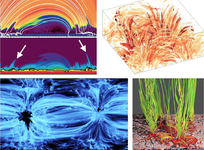
Figure 3: A selection of results from multidimensional MHD coronal models. Clockwise from upper-left, the illustrated quantities are: (1) temperature, with magnetic field lines in white (top), and density (bottom) from Martínez-Sykora et al. (2017), (2) Joule heating rate from Kanella & Gudiksen (2017), (3) impulsively heated magnetic field lines from Amari et al. (2015), and (4) synthesized emission measure from Rempel (2017). The Amari et al. (2015) image was published on phys.org on 11 June 2015, with credit to Tahar Amari (Centre de Physique Théorique, CNRS-Ecole Polytechnique, France). These simulations are all driven by large-scale surface motions, such that their heating tends to be dominated by DC-type processes.

At the spatial scales resolved by the current generation of simulations (e.g., about 0.1 Mm), there seems to be agreement that DC-type footpoint braiding is the dominant process, and that it is indeed sufficient to supply the necessary coronal heating. However, these coarsely resolved models tend to suppress the generation of rapid fluctuations such as AC-type waves or MHD turbulence. Thus, another class of multidimensional numerical experiments has arisen that aims to follow the internal structure of just one macroscopic coronal loop, but with greater internal detail (e.g., van Ballegooijen et al., 2011; Perez & Chandran, 2013; Matsumoto, 2018). When the photospheric footpoints of these models are driven at appropriately small space and time scales, they tend to produce waves and turbulence that dissipate rapidly enough to heat the corona at reasonable levels. When these models are driven slowly (i.e., more commensurate with the DC driving in the coarser simulations), they tend not to produce much heating (van Ballegooijen et al., 2014). However, the single-loop simulations do not include the effects of neighboring footpoints that become tangled and twisted up with one another on larger cross-field scales. Thus, it is unclear whether a future simulation that resolves both sets of scales simultaneously will be dominated by AC or DC heating.

5.5 The Coronal Plasma State

In order to determine which theoretical heating mechanisms apply to the real solar corona, model predictions must be compared to observational data. A variety of approaches has been taken, and some combination of forward modeling (i.e., taking the model output and synthesizing artificial observations) and inverse modeling (i.e., processing data from the telescope to determine the plasma properties in the corona) must be employed. A key link in this chain is to understand how a given heating rate $Q$ gives rise to a known variation of temperature and density along a magnetic field line. In general, the corona finds an equilibrium solution that balances coronal heating with transport and loss terms associated with heat conduction, radiative emission, and enthalpy transport due to flows. For coronal loops, these solutions typically have a maximum temperature $T_{\rm max}$ at the loop apex and a basal gas pressure $P_{0}$ that varies slowly along the loop because of the large scale height. [] RTVRosner, Tucker, & Vaiana The much-cited RTV model (Rosner et al., 1978) provides analytic scaling laws for these quantities under the assumptions of constant $Q$, classical Spitzer heat conductivity, and a radiative cooling rate that scales as $\rho^{2}T^{-m}$. The RTV scaling laws are given by

$$T_{\rm max}\,\propto\,Q^{2/7}L^{4/7}\,\,,\,\,\,\,\,\,\,P_{0}\,\propto\,Q^{(11+2m)/14}L^{(4+2m)/7}\,\,,$$ (5)

and, for simplicity, the normalizing constants in these expressions are not shown. Note that a factor of ten change in $Q$ produces a much smaller (factor of $10^{2/7}\approx 2$) change in $T_{\rm max}$ because conduction acts as a kind of “thermostat” to smooth out the effects of coronal heating. Subsequent work has resulted in modified scaling laws that allow for spatial variability in the pressure and heating rate (see, e.g., Serio et al., 1981; Aschwanden & Schrijver, 2002; Martens, 2010).

With the advent of efficient computers, it has become possible to perform large-scale pixel-by-pixel comparisons between observed coronal images and synthesized trial images created with a range of guesses about the heating rate. Different dependences of $Q$ on quantities such as the coronal field strength $B$ and the loop length $L$ produce very different patterns of synthetic EUV and X-ray emission (Mandrini et al., 2000; Schrijver et al., 2004; Lundquist et al., 2008; Fludra et al., 2017). For example, Schrijver et al. (2004) found a best fit with observations for $Q\propto B/L^{2}$, which is roughly equivalent to ${\cal E}\approx\Lambda^{2}\Theta$, or the prediction from the Parker (1983) braiding model. For different data, Lundquist et al. (2008) found a better fit for $Q\propto B/L$, which comes closer to some of the scalings described above for Alfvén waves (${\cal E}\approx\Lambda\Theta$). Warren & Winebarger (2006) pointed out a possible ambiguity between these two scalings, depending on whether the magnetic field is taken at the coronal base ($B_{0}$) or averaged over the loop ($\bar{B}$), because observations tend to show $\bar{B}\propto B_{0}/L$. Of course, the dependence of $Q$ on other parameters besides $B$ and $L$ should not be ignored. Tiwari et al. (2017) studied the importance of convective suppression in sunspots to find that bright coronal loops occur when there is at least one footpoint rooted in the penumbra (high $v_{\perp}$), but there is virtually no coronal emission when both feet are rooted in the dark umbra (very low $v_{\perp}$).

Figure 4 shows example time-steady solutions for temperature and density for a sequence of closed loops with different lengths and for an example open-field case (Cranmer et al., 2007). In the chromosphere ($T<10^{4}$ K), the stable solution to the energy conservation equation comes mainly from a balance between imposed heating and radiative losses. However, when the density drops to a point at which radiative cooling can no longer balance the heating, a rapid transition occurs to coronal conditions that must also involve heat conduction. The plotted loop models were meant to emulate empirical model-atmosphere sequences such as Vernazza et al. (1981) and Fontenla et al. (2011). Our basic assumption was that $Q\propto L^{-3}$, which is consistent with a range of heating models from Table 1. If we also assume $B\propto 1/L$ (Jain & Mandrini, 2006), one can obtain $Q\propto L^{-3}$ from Parker (1983) or Dmitruk & Gómez (1999) or just a constant Poynting efficiency ${\cal E}$. The loop models in Figure 4 also used $m=0.5$ in Equation 5, analytic expressions for $T(r)$ in the corona from Martens (2010), and numerical solutions for the chromosphere similar to those of Cranmer et al. (2007).

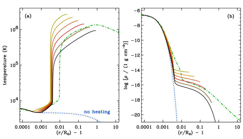
Figure 4: Dependence of temperature (a) and mass density (b) on height above the solar surface (i.e., with $r=R_{\odot}$ denoting the photosphere, and heights expressed in units of solar radii) for several representative models. Solid curves show closed field-line loops with a range of lengths $L$ between 30 and 1200 Mm. The green dot-dashed curve shows an open-field coronal hole model from Cranmer et al. (2007). Another open-field model with no coronal heating whatsoever is also shown (i.e., pure radiative equilibrium; blue dotted curve).

Computers also allow spatial and time variability in the heating rate to be incorporated into synthetic observations. Useful insights have come from zero-dimensional (e.g., Klimchuk et al., 2008), one-dimensional (Polito et al., 2018), and three-dimensional (Mok et al., 2005) forward modeling with time- and space-dependent heating. The multidimensional simulations discussed in Section 5.4 naturally produce a rapid decline in the mean heating rate as a function of increasing height, with $Q\propto\exp(-z/s_{\rm H})$ and $s_{\rm H}\approx 5$–15 Mm (Peter, 2015). Including this effect alone can reproduce many of the observed properties of the solar corona, such as evolving loops, larger-than-expected densities, and coronal rain (Mok et al., 2016; Winebarger et al., 2016). Footpoint-stressing models require a finite time between events to allow for energy to build up in the magnetic field (López Fuentes & Klimchuk, 2016). Incorporating the time dependence of the heating can also produce evolving loops and the observed emission measure distribution (Cargill et al., 2015; Van Doorsselaere et al., 2018). Finally, the heating rate may be unequal at the two footpoints of a loop, and this kind of imbalance can drive so-called siphon flows from one end to the other. These have been discussed theoretically for many decades, but observed only rarely (see, e.g., Huang et al., 2015).

Lastly, it is important to note that the coronal plasma state may not always be described most accurately as a classical MHD fluid. The creation of a hot corona involves taking some of the cold particles from below and increasing their most-probable random speeds; i.e., broadening their kinetic velocity distributions. The shapes of these distributions may not always remain Maxwellian, even in regions where Coulomb collisions are frequent (Meyer-Vernet, 2007; Echim et al., 2011; Dudík et al., 2017). It has been proposed that a power-law tail of suprathermal particles may exist down in the chromosphere, and the fraction of such particles that escape to larger heights may be enhanced relative to the particles in the core Maxwellian distribution. This velocity filtration effect could conceivably produce a hot corona without the need for any other heating (see, e.g., Scudder, 1992). However, it still requires some mechanism to give thermal energy to the particles—and thus generate suprathermal tails—in the chromosphere. It is unclear what this mechanism could be and how strong it would have to be to prevent collisions and radiative losses from driving these particles back into thermal Maxwellian equilibrium.

6 THE CORONA-HELIOSPHERE CONNECTION

6.1 Physical Processes

Parker’s (1958, 1963) original idea of a gas-pressure-driven outflow is still believed to be responsible for much of the observed acceleration of the solar wind along open magnetic field lines. Thus, the ultimate explanation for the existence of the heliosphere must come back to an understanding of the coronal heating problem. In fact, the determination of one key property of the wind—the total rate of mass loss $\dot{M}$—is so directly related to coronal heating that it sidesteps Parker’s solution of the momentum equation entirely. The solar mass-loss rate appears to be set by the same thermal energy balance that is responsible for setting the base pressure $P_{0}$ in coronal loops. In other words, in both closed and open regions, the dense reservoir of the chromosphere releases as much plasma as necessary to reach a time-steady balance between heating, radiative losses, thermal conduction, and any enthalpy flux due to flows (e.g., Hammer, 1982; Leer et al., 1982; Hansteen & Leer, 1995).

Even without adding any other physical processes besides Parker’s basic gas-pressure gradient, the nature of the acceleration depends very much on the spatial distribution of coronal heating. Holzer & Axford (1970) and Owocki (2004) summarized the behavior of solar wind models with effectively polytropic equations of state; i.e., $P\propto\rho^{\gamma}$. Figure 5a shows a series of models with a range of specified $\gamma$ exponents. The original (Parker, 1958) isothermal model was equivalent to $\gamma=1$. The existence of a high temperature that extends to large distances implies a large gas-pressure gradient that can continue to accelerate the flow in perpetuity. Higher values of $\gamma$ imply a more rapidly declining temperature with increasing distance (i.e., with decreasing density). Holzer & Axford (1970) showed that one requires $\gamma<1.5$ in order to maintain an outflow that accelerates through the critical point. Note that the adiabatic value of $\gamma$ appropriate for a monatomic gas (i.e., $\gamma=5/3$) does not allow for an accelerating solar wind. This means that some kind of non-adiabatic energy addition—either in the form of extended coronal heating or strong heat conduction—must exist to prevent adiabatic cooling and to maintain the observed acceleration.

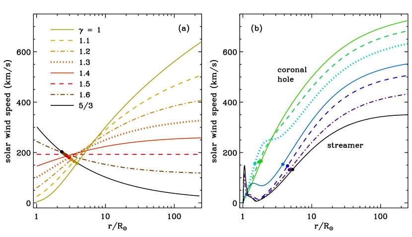
Figure 5: Illustrations of one-dimensional models of solar wind acceleration. (a) Polytropic solutions in spherical geometry, each computed with $T=1.5$ MK at the critical point. (b) Self-consistent models of coronal heating via anisotropic MHD turbulence, for a selection of open field lines from an axisymmetric solar-minimum magnetic geometry (Cranmer et al., 2007). In both panels, solid circles denote the locations of Parker’s critical point. Note that 1 AU = 215 $R_{\odot}$.

Although there are still gaps in our observational knowledge of the coronal temperature in regions of solar wind acceleration (e.g., Kohl et al., 2006), we know enough to make the claim that Parker’s gas-pressure gradient must sometimes be supplemented by other sources of acceleration. Fast solar wind streams associated with coronal holes have speeds that ultimately reach 700–900 km s^-1 at 1 AU. This is difficult to explain with observed constraints on gas-pressure gradients due to the dominant protons, electrons, and alpha particles. Some have proposed that large-amplitude MHD waves exert enough of a time-averaged ponderomotive force to provide the extra required acceleration (Alazraki & Couturier, 1971; Jacques, 1977). There can also be a strong additional outward force due to temperature anisotropies in the dominant particle velocity distributions. When the temperature perpendicular to the magnetic field exceeds that in the direction parallel to the field, there is an effective magnetic-mirror type force that points in the direction of weakening magnetic field strength (i.e., outward from the Sun; see Hollweg & Isenberg 2002). Both supplemental sources of acceleration have been proposed to be present naturally in coronal holes, since these regions tend to exhibit strong MHD-wave activity and temperature anisotropies (Marsch, 2006).

Numerical models that account for many of the above processes have been successful in predicting the observed properties of fast and slow wind streams (e.g., Ofman, 2010; Lionello et al., 2014; Gombosi et al., 2018; Shoda et al., 2018). Figure 5b shows a set of results from Cranmer et al. (2007) that reproduces the latitudinal variation of solar wind properties at solar minimum. This model solves the mass, momentum, and energy conservation equations along one-dimensional flux tubes of arbitrary geometry using the reflection-driven cascade model described in Section 5.3.2. For the highest-speed (open-field polar coronal hole) model, the output values of temperature and density are shown in Figure 4. The slowest-wind models correspond to streamer or cusp geometries that also have enhanced (i.e., active-region-like) magnetic fields at the base. In the models, this stronger field produces a small-scale source of additional time-steady acceleration, which in turn produces a local maximum in the wind speed of about 100 km s^-1 in the low corona. This may help explain the fan-like outflows of similar magnitude that have been seen in active regions by Hinode (Harra et al., 2008; Baker et al., 2009; van Driel-Gesztelyi et al., 2012).

In addition to the wave/turbulence-based models discussed above, there have been other ideas proposed for the origin of mass, momentum, and energy in the solar wind. High-resolution observations of dynamic structures in the chromosphere (e.g., spicules and jets) show that the solar atmosphere is filled with rapid, collimated surges of plasma that flow both up and back down. It has been suggested that a fraction of this plasma becomes heated to coronal temperatures and thus can be injected directly into the solar wind (see, e.g., Moore et al., 2011; McIntosh, 2012). This scenario is similar to others that emphasize the importance of flux emergence and interchange reconnection in the supergranular network. At scales of order 5–30 Mm in the low corona, emerging magnetic bipoles tend to advect towards the edges of the network and undergo magnetic reconnection with neighboring flux systems. This process can transfer hot plasma from closed to open magnetic field lines and thus drive jet-like pulses of plasma into the solar wind (Fisk et al., 1999; Yang et al., 2013). Jets are indeed observed both in the chromosphere and corona, but they tend to be identifiable because they occur intermittently in time with a small filling factor in volume. Thus, it is uncertain whether these kinds of impulsive events are responsible for the majority of the plasma comprising the corona and solar wind.

6.2 Mapping and Forecasting

A long-term objective of solar and heliospheric physics has been to make accurate predictions of the spatial and temporal distribution of solar wind plasma properties (usually organized by speed) based on the state of the corona. We know of several strong correlations between the coronal magnetic field and the solar wind at 1 AU, but there are still uncertainties about the relative contributions of different structures. The fastest streams (i.e., speeds exceeding 600 km s^-1) tend to be associated with the central regions of large, unipolar coronal holes. Slow solar wind has been associated with multiple coronal features—e.g., active regions, helmet streamers, pseudostreamers, outer boundaries of coronal holes, and transient jets associated with interchange reconnection (see Luhmann et al., 2002; Brooks et al., 2015; Abbo et al., 2016)—but the relative contributions from these sources remain difficult to quantify. [] Helmet streamerBipolar magnetic fields stretched out into the solar wind, with footpoints of opposite polarity PseudostreamerMultipolar magnetic fields stretched into the solar wind, with footpoints of like polarity There has also been increased interest in how the topological properties of the Sun’s magnetic field may relate to the occurrence of slow solar wind. Specifically, Antiochos et al. (2011) found that there is often a complex web-like collection of magnetic separatrix surfaces, mainly associated with pseudostreamers, that corresponds to a 20^∘ to 30^∘ wide band of slow solar wind around the heliospheric current sheet. Parcels of slow wind that come from different coronal sources appear to have different patterns of frozen-in ionization states and FIP elemental fractionation (see Section 4). These trends are sometimes used to argue for the prevalance of magnetic reconnection in the source regions of the slow wind, but there are also wave/turbulence models that predict similar patterns (see, e.g., Cranmer et al., 2017).

Attempts to accurately locate the coronal field lines that connect to specific fast or slow wind streams are often hampered by the existence of stochastic processes that can mix and tangle the field lines on a wide range of scales. Such processes include small-scale MHD turbulence (Ragot, 2009) and large-scale stream-stream interactions (Richardson, 2018), and their presence can lead to a loss of information about where on the Sun a given stream came from. Because of these ambiguities, there is a lack of agreement about whether it even makes sense to classify the solar wind into discrete states or types, and if so, how those classifications should depend on in situ measurements or the successful identification of coronal source regions (e.g., Wang et al., 2009; Crooker et al., 2014; Stakhiv et al., 2016; Neugebauer et al., 2016).

Despite the difficulties in associating solar wind streams with specific coronal sources, there is a well-established empirical relationship between the speed of a parcel of solar wind at 1 AU and the inferred topological behavior of its approximate magnetic footpoint. Levine et al. (1977) and Wang & Sheeley (1990) discovered an inverse correlation between the wind speed and the degree of superradial flux-tube expansion (i.e., the amount of trumpet-like growth of an area traced out by the tips of field lines in a compact bundle) between the photosphere and a reference point at a radial distance of about 2.5 $R_{\odot}$. This relationship, together with subsequent refinements (see also Arge & Pizzo, 2000; Riley et al., 2015), is typically called the WSA model (after Wang, Sheeley, & Arge), and it has evolved into an integral part of modern-day operational space-weather forecasting. [] WSAWang, Sheeley, & Arge Kovakenko (1981) and Wang & Sheeley (1991) proposed independently that the physical origin of this effect is related to the existence of Alfvén waves at the coronal base. Consider a situation in which the upward energy flux of waves is the same at every point on the solar surface. A parcel of plasma up in the corona with a low superradial expansion factor collects wave energy from a larger patch of the surface than does a parcel of the same size associated with a high superradial expansion factor. Thus, the low-expansion regions will have the most vigorous waves and turbulent fluctuations, the most wave-driven coronal heating, and thus the most intense solar wind acceleration. It is probably no coincidence that the central regions of coronal holes exhibit the lowest superradial expansion factors.

7 BROADER CONTEXT

The Sun is the closest star to the Earth, and for many years it has served as a template for our understanding of the physical processes that occur in other stars and even more exotic astrophysical environments. This is especially true for the observational signatures of magnetic fields, hot coronae, and outflowing winds around cool stars, all of which have been traditionally difficult to detect and characterize (see, e.g., Dupree, 1986; Sonett et al., 1991; Pagano et al., 2006; Brun et al., 2015; Linsky, 2017). The most luminous stars tend to have quite high rates of mass loss and dense circumstellar envelopes, so spectroscopic signatures of their winds are often quite clear. On the other hand, main-sequence stars similar to the Sun have much more tenuous winds. At present, even indirect mass-loss measurements are possible only for our nearest stellar neighbors, for which interstellar absorption has not obscured subtle signatures of their astrospheric emission (i.e., pileup of neutral hydrogen due to winds interacting with the local interstellar medium; see Wood  2018). Also, the growth of techniques such as Zeeman Doppler Imaging (e.g., See et al., 2017) and an increased utilization of high-resolution X-ray spectroscopy (Güdel & Nazé, 2010) have led to much more being known about the magnetic fields and coronal activity of solar-type stars.

Figure 6 summarizes recent measurements of mass-loss rates and the regions of parameter space in which coronal X-rays are typically seen. The dominant trend appears to be that more luminous stars have larger mass-loss rates. This agrees broadly with the idea that each step in the long chain of processes discussed above—from convective energy transport below the photosphere to coronal heating above the photosphere—scales with the total available energy flux flowing through the star (see also Reimers, 1975; Schröder & Cuntz, 2005). The stars most similar to the Sun are those in the lower-left region of the plot, with high surface gravities and correspondingly small scale heights. In the upper atmospheres of these stars, the density drops rapidly to a point below which radiative cooling cannot balance the heating (see Section 5.5) and a million-degree corona occurs inevitably. These stars exhibit X-ray and UV emission similar to the Sun’s. However, as one moves to the upper-right part of the plot, the stellar radii increase, the surface gravities become lower, and thus the atmospheric scale heights become larger. Combined with the high rates of mass loss, this leads to high-density chromospheres that extend for several stellar radii, and there is no runaway to a hot corona. For such stars, Holzer et al. (1983) proposed the existence of cold wave-driven winds (see also Suzuki, 2007; Cranmer & Saar, 2011). There also appears to be a narrow region of hybrid stellar parameters between the hot and cold domains (Linsky & Haisch, 1979); some these stars display spectra characteristic of a “warm” transition region (Hartmann et al., 1980) and others show UV signatures of weak coronae despite the lack of X-rays (Ayres et al., 1997, 2003).

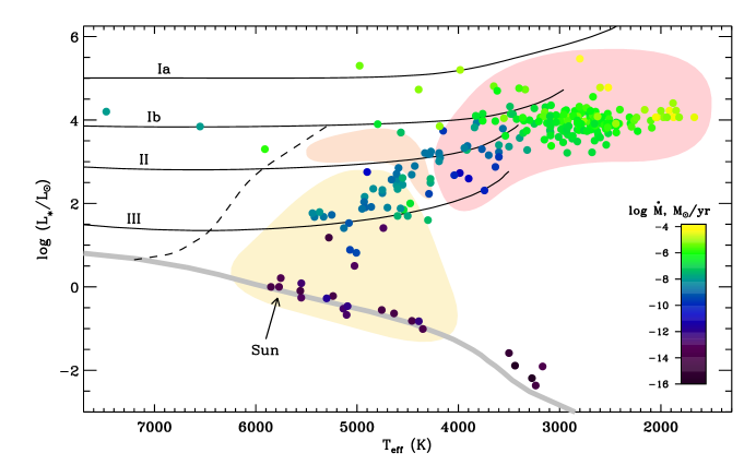
Figure 6: Cool-star Hertzsprung-Russell diagram. Symbol colors correspond to observed mass-loss rates (Cranmer & Saar, 2011; Wood, 2018). Also shown: zero-age main sequence (thick gray curve), empirical luminosity classes (solid black curves; de Jager & Nieuwenhuijzen 1987), and a boundary between stars with and without subsurface convection (dashed curve; Gray & Nagel 1989). Larger regions, from lower-left to upper-right, denote Sun-like stars with hot coronae (yellow), warm/hybrid stars with weak or sporadic coronal signatures (orange), and cool giants/supergiants without coronae (red); see, e.g., Linsky & Haisch (1979); Ayres et al. (2003).

There are several important avenues of study in astrophysics and planetary science that depend on (or have developed from) our understanding of the physical processes that produce the solar corona and wind. The following list gives a small and unrepresentative selection.

1. In the first few million years after the Sun’s formation, its enhanced mass outflow and UV radiation were probably important factors in dissipating the primeval atmospheres of the inner planets (Lammer et al., 2012; Jakosky et al., 2018). For planets that orbit much closer to their host stars than those in our solar system, even weak winds (e.g., $\dot{M}\approx 10^{-14}$ $M_{\odot}$ yr^-1) may have substantial impacts. The effects of both coronal emission and stellar mass loss need to be taken into account to accurately determine the age-dependent masses, densities, and magnetic fields of many types of planets (e.g., Heyner et al., 2012; Garraffo et al., 2017).

2. For young stars, the high-energy coronal radiation responsible in part for eroding away accretion disks seems to be dominated by strong stellar flares. Extrapolating from the present-day Sun, these so-called super-flares may also be responsible for strong CME-type eruptions of mass and magnetic flux (Aarnio et al., 2012). However, there has not yet been a clear and unambiguous detection of a stellar CME, and it is suspected that strong magnetic fields may often exert enough of a binding tension force to prevent eruptive material from escaping (Alvarado-Gómez et al., 2018). Nevertheless, strong ambient stellar mass loss is observed from young stars, and the presence of a dense wind can act to shield inner circumstellar regions from galactic cosmic rays. This can have a strong impact on the evolution of a star’s protoplanetary disk (Cleeves et al., 2015).

3. Photospheric elemental abundances of stars can be used as diagnostics of internal processes such as convective mixing and radiative acceleration, and they are key to the accurate interpretation of asteroseismic data (see, e.g., Allende Prieto, 2016). At layers above the photosphere, cool-star spectroscopy reveals a diversity of abundance patterns, including sometimes a solar-like FIP effect (enhanced low-FIP abundances) and sometimes an inverse-FIP effect (depleted low-FIP abundances). There is still no complete theory to explain these variations, but it has been proposed that they arise due to differences in sunspot/starspot coverage and its impact on wave propagation and mode conversion in solar/stellar chromospheres (Laming, 2015; Doschek & Warren, 2017).

4. Over billions of years, stellar winds return metal-enriched gas back to the interstellar medium to affect subsequent generations of stars (Willson, 2000; Dale, 2015). Fundamental physical processes such as MHD turbulence, magnetic reconnection, Taylor relaxation, and kinetic particle acceleration are being invoked with increasing frequency in models of the interstellar medium (Burkhart et al., 2009), accretion flows around supermassive black holes (Rowan et al., 2017), and galaxy clusters (Bambic et al., 2018).

8 CONCLUSIONS AND FUTURE PROSPECTS

The goal of this paper has been to review some key aspects of historical and recent advances in our understanding the corona and solar wind. Considerable progress has been made over the last few decades in improving both the quality and quantity of the observational data. Theoretical models and computer simulations also continue to proliferate and explain an increasing amount of what we observe. The solution of the intertwined problems of coronal heating and solar wind acceleration thus requires us to winnow down the list of proposed theories and determine which one (or ones) are truly dominant on the actual Sun. If these competing ideas could be formalized as a complete set of mutually exclusive hypotheses, then something like Bayesian reasoning could be employed to evaluate their relative likelihoods (see, e.g., Sturrock, 1973).

Another route toward identifying and characterizing the most important physical processes for coronal heating is to improve the accuracy and dynamic range of the simulations. In Section 5.4 we discussed the goal of including a broader range of footpoint-driving motions and coronal field-line interactions in multidimensional MHD simulations. Only when both AC and DC processes (as well as turbulence and Taylor relaxation) are allowed to interact with one another without numerical constraints will the most realistic consequences emerge. Going beyond single MHD simulations—either into the realm of nonequilibrium kinetic physics (e.g., Cerri et al., 2017) or into the probabilistic arena of large ensembles of simulations (Owens & Riley, 2017)—is also becoming possible. Ultimately, it is crucial to extract from the simulations some key physical principles that make the results comprehensible to human beings. This may take the form of improved coronal-heating scaling laws (e.g., Bourdin et al., 2016) or, once the simulations reveal which effects are important and which are ignorable, it may result in completely new analytic theories.

One of the results of numerical simulations must be to identify observables that can discriminate between the competing theories and drive the next generation of solar observations. Though a wealth of data currently exists for the Sun, multiple theoretical mechanisms can be shown to be consistent with these observations. Undoubtedly the upcoming data from the Parker Solar Probe (Fox et al., 2016) and the Daniel K.  Inouye Solar Telescope (Tritschler et al., 2016) will help to differentiate between different mechanisms. Better measurements of the outer corona (i.e., the extended acceleration region of the solar wind) are helping to bridge the gap between the traditionally separate communities of solar and space physics (see, e.g., Kohl et al., 2006, 2008; DeForest et al., 2018). Improving the spatial resolution of observations and increasing the temperature sensitivity (especially at higher temperatures) is undoubtedly important as well. Migrating successful suborbital instruments (such as Hi-C, FOXSI, and EUNIS) to orbital platforms—and continuing to test novel techniques through the sounding rocket program—will ensure that long-baseline data sets have state-of-the-art capabilities.

Although the identification of the processes that drive coronal heating is interesting for its own sake, this problem exists inside a broader research ecosystem. Thompson (2014) identified two of the highest-level unsolved problems in solar physics: (1) improving the predictability of space weather, and (2) modeling solar/stellar MHD dynamos from first principles. Solving the first problem obviously requires improving our understanding of coronal heating and solar wind acceleration. Forecasting techniques based on empirical correlations (e.g., the WSA model) have been successful, but including more of the relevant physics can only lead to improvements (see, e.g., Cranmer et al., 2017). Solving the second problem listed above may also depend on our knowledge about the mechanisms that produce the corona and heliosphere. For example, it has been proposed that mass loss in the form of CMEs must play an important role in a solar-type dynamo by shedding magnetic helicity that would otherwise build up in the convection zone (Blackman & Field, 2000; Brandenburg, 2007). In addition, the long-term evolution of a stellar dynamo depends on the star’s rotational history, and that in turn depends on the loss of mass and angular momentum in the wind (Weber & Davis, 1967; Bouvier et al., 2014; Metcalfe & van Saders, 2017).

DISCLOSURE STATEMENT

The authors are not aware of any affiliations, memberships, funding, or financial holdings that might be perceived as affecting the objectivity of this review.

References

- Aarnio et al. (2012) Aarnio AN, Matt SP, Stassun KG. 2012. Ap. J. 760:9
- Abbo et al. (2016) Abbo L, Ofman L, Antiochos SK, et al. 2016. Space Sci. Rev. 201:55–108
- Alazraki & Couturier (1971) Alazraki G, Couturier P. 1971. Astron. Astrophys. 13:380–389
- Alfvén (1941) Alfvén H. 1941. Arkiv Math. Astron. Fysik (Band 27A), 25:1–23
- Allende Prieto (2016) Allende Prieto C. 2016. Living Rev. Solar Phys. 13:1
- Alvarado-Gómez et al. (2018) Alvarado-Gómez JD, Drake JJ, Cohen O, Moschou SP, Garraffo C. 2018. Ap. J. 862:93
- Amari et al. (2015) Amari T, Luciani JF, Aly JJ. 2015. Nature 522:188–191
- Antiochos et al. (2011) Antiochos SK, Mikić Z, Titov VS, Lionello R, Linker JA. 2011. Ap. J. 731:112
- Antolin & Rouppe van der Voort (2012) Antolin P, Rouppe van der Voort L. 2012. Ap. J. 745:152
- Arge & Pizzo (2000) Arge CN, Pizzo VJ. 2000. J. Geophys. Res. 105:10465–10480
- Aschwanden (2006) Aschwanden MJ. 2006. Physics of the Solar Corona: An Introduction with Problems and Solutions, 2nd ed. Chichester, UK: Springer-Praxis
- Aschwanden & Schrijver (2002) Aschwanden MJ, Schrijver CJ. 2002. Ap. J. Suppl. Ser. 142:269–283
- Aschwanden et al. (2001) Aschwanden MJ, Schrijver CJ, Alexander D. 2001. Ap. J. 550:1036–1050
- Athay & White (1978) Athay RG, White OR. 1978. Ap. J. 226:1135–1139
- Axford et al. (1999) Axford WI, McKenzie JF, Sukhorukova GV, et al. 1999. Space Sci. Rev. 87:25–41
- Ayres et al. (2003) Ayres TR, Brown A, Harper GM. 2003. Ap. J. 598:610–625
- Ayres et al. (1997) Ayres TR, Brown A, Harper GM, et al. 1997. Ap. J. 491:876–884
- Baker et al. (2009) Baker D, van Driel-Gesztelyi L, Mandrini CH, Démoulin P, Murray MJ. 2009. Ap. J. 705:926–935
- Bambic et al. (2018) Bambic CJ, Morsony BJ, Reynolds CS. 2018. Ap. J. 857:84
- Bandyopadhyay et al. (2018) Bandyopadhyay R, Chasapis A, Chhiber R, et al. 2018. Ap. J. Suppl. Ser. in press, arXiv:1807.06140
- Baumbach (1937) Baumbach S. 1937. Astron. Nachr. 263:121–134
- Beck et al. (2012) Beck C, Rezaei R, Puschmann KG. 2012. Astron. Astrophys. 544:A46
- Belcher & Davis (1971) Belcher JW, Davis L Jr. 1971. J. Geophys. Res. 76:3534–3563
- Bello González et al. (2010) Bello González N, Franz M, Martínez Pillet V, et al. 2010. Ap. J. Lett. 723:L134–L138
- Biermann (1951) Biermann L. 1951. Z. Astrophysik 29:274–286
- Billings (1966) Billings DE. 1966. A Guide to the Solar Corona. New York: Academic Press
- Birkeland (1908) Birkeland K. 1908. The Norwegian Aurora Polaris Expedition, 1902-–1903. New York and Christiania: H. Aschehoug
- Blackman & Field (2000) Blackman EG, Field GB. 2000. MNRAS 318:724–732
- Blake et al. (1963) Blake RL, Chubb TA, Friedman H, Unzicker AE. 1963. Ap. J. 137:3–15
- Bourdin et al. (2016) Bourdin PA, Bingert S, Peter H. 2016. Astron. Astrophys. 589:A86
- Bouvier et al. (2014) Bouvier J, Matt SP, Mohanty S, et al. 2014 In Protostars and Planets VI, ed. H Beuther, RS Klessen, CP Dullemond, T Henning, pp. 433–450. Tucson: U. Arizona Press
- Brandenburg (2007) Brandenburg A. 2007. Highlights Astron. 14:291–292
- Brooks et al. (2015) Brooks DH, Ugarte-Urra I, Warren HP. 2015. Nature Comm. 6:5947
- Brooks & Warren (2016) Brooks DH, Warren HP. 2016. Ap. J. 820:63
- Browning & Priest (1986) Browning PK, Priest ER. 1986. Astron. Astrophys. 159:129–141
- Brun et al. (2015) Brun AS, García RA, Houdek G, Nandy D, Pinsonneault M. 2015. Space Sci. Rev. 196:303–356
- Bruno & Carbone (2013) Bruno R, Carbone V. 2013. Living Rev. Solar Phys. 10:2
- Burkhart et al. (2009) Burkhart B, Falceta-Gonçalves D, Kowal G, Lazarian A. 2009. Ap. J. 693:250–266
- Burlaga et al. (1996) Burlaga LF, Ness NF, Belcher JW, Lazarus AJ, Richardson JD. 1996. Space Sci. Rev. 78:33–42
- Cargill et al. (2015) Cargill PJ, Warren HP, Bradshaw SJ. 2015. Phil. Trans. Roy. Soc. A 373:20140260
- Carlsson et al. (2007) Carlsson M, Hansteen VH, De Pontieu B, et al. 2007. Pub. Astron. Soc. Japan 59:S663–S668
- Carlsson & Stein (1997) Carlsson M, Stein RF. 1997. Ap. J. 481:500–514
- Carrington (1859) Carrington RC. 1859. MNRAS 20:13–15
- Cerri et al. (2017) Cerri SS, Servidio S, Califano F. 2017. Ap. J. Lett. 846:L18
- Chae et al. (2002) Chae J, Poland AI, Aschwanden MJ. 2002. Ap. J. 581:726–735
- Chamberlain (1961) Chamberlain JW. 1961. Ap. J. 133:675–687
- Chandran et al. (2015) Chandran BDG, Perez JC, Verscharen D, Klein KG, Mallet A. 2015. Ap. J. 811:50
- Chapman (1918) Chapman S. 1918. Proc. Roy. Soc. A 95:61–83
- Cheung & Isobe (2014) Cheung MCM, Isobe H. 2014. Living Rev. Solar Phys. 11:1
- Cirtain et al. (2013) Cirtain JW, Golub L, Winebarger AR, et al. 2013. Nature 493:501–503
- Cleeves et al. (2015) Cleeves LI, Bergin EA, Qi C, Adams FC, Öberg KI. 2015. Ap. J. 799:204
- Coleman (1968) Coleman PJ Jr. 1968. Ap. J. 153:371–388
- Cranmer (2014) Cranmer SR. 2014. Ap. J. Suppl. Ser. 213:16
- Cranmer et al. (2017) Cranmer SR, Gibson SE, Riley P. 2017. Space Sci. Rev. 212:1345–1384
- Cranmer & Saar (2011) Cranmer SR, Saar SH. 2011. Ap. J. 741:54
- Cranmer et al. (2007) Cranmer SR, van Ballegooijen AA, Edgar RJ. 2007. Ap. J. Suppl. Ser. 171:520–551
- Crooker et al. (2014) Crooker NU, McPherron RL, Owens MJ. 2014. J. Geophys. Res. 119:4157–4163
- Cuntz et al. (2007) Cuntz M, Rammacher W, Musielak ZE. 2007. Ap. J. Lett. 657:L57–L60
- Dahlburg et al. (2016) Dahlburg RB, Einaudi G, Taylor BD, et al. 2016. Ap. J. 817:47
- Dale (2015) Dale JE. 2015. New Astron. Rev. 68:1–33
- Daughton & Roytershteyn (2012) Daughton W, Roytershteyn V. 2012. Space Sci. Rev. 172:271–282
- de Jager & Nieuwenhuijzen (1987) de Jager C, Nieuwenhuijzen H. 1987. Astron. Astrophys. 177:217–227
- DeForest et al. (2018) DeForest CE, Howard RA, Velli M, Viall N, Vourlidas A. 2018. Ap. J. 862:18
- Del Zanna & Mason (2018) Del Zanna G, Mason HE. 2018. Living Rev. Solar Phys. 15:5
- Dessler (1967) Dessler AJ. 1967. Rev. Geophys. 5:1–41
- Dmitruk & Gómez (1999) Dmitruk P, Gómez DO. 1999. Ap. J. Lett. 527:L63–L66
- Doschek & Warren (2017) Doschek GA, Warren HP. 2017. Ap. J. 844:52
- Drake et al. (2009) Drake JF, Swisdak M, Phan TD, et al. 2009. J. Geophys. Res. 114:A05111
- Druckmüller et al. (2006) Druckmüller M, Rušin V, Minarovjech M. 2006. Contrib. Astron. Obs. Skalnaté Pleso 36:131–148
- Dudík et al. (2017) Dudík J, Dzifčáková E, Meyer-Vernet N, et al. 2017. Solar Phys. 292:100
- Dupree (1986) Dupree AK. 1986. Annu. Rev. Astron. Astrophys. 24:377–420
- Echim et al. (2011) Echim MM, Lemaire J, Lie-Svendsen Ø. 2011. Surveys in Geophys. 32:1–70
- Edlén (1943) Edlén B. 1943. Z. Astrophysik 22:30–64
- Elsasser (1950) Elsasser WM. 1950. Phys. Rev. 79:183
- Feldman (1992) Feldman U. 1992. Physica Scripta 46:202–220
- Fisher et al. (1998) Fisher GH, Longcope DW, Metcalf TR, Pevtsov AA. 1998. Ap. J. 508:885–898
- Fisk et al. (1999) Fisk LA, Schwadron NA, Zurbuchen TH. 1999. J. Geophys. Res. 104:19765–19772
- Fletcher et al. (2011) Fletcher L, Dennis BR, Hudson HS, et al. 2011. Space Sci. Rev. 159:19–106
- Fludra et al. (2017) Fludra A, Hornsey C, Nakariakov VM. 2017. Ap. J. 834:100
- Fontenla et al. (2011) Fontenla JM, Harder J, Livingston W, Snow M, Woods T. 2011, J. Geophys. Res. 116:D20108
- Fox et al. (2016) Fox NJ, Velli MC, Bale SD, et al. 2016. Space Sci. Rev. 204:7–48
- Froment et al. (2017) Froment C, Auchère F, Aulanier G, et al. 2017. Ap. J. 835:272
- Galsgaard & Nordlund (1996) Galsgaard K, Nordlund Å. 1996. J. Geophys. Res. 101:13445–13460
- Garraffo et al. (2017) Garraffo C, Drake JJ, Cohen O, Alvarado-Gómez JD, Moschou SP. 2017. Ap. J. Lett. 843:L33
- Goldreich & Sridhar (1995) Goldreich P, Sridhar S. 1995. Ap. J. 438:763–775
- Goldstein et al. (2015) Goldstein ML, Escoubet P, Hwang KJ, et al. 2015. J. Plasma Phys. 81:325810301
- Golub & Pasachoff (2010) Golub L, Pasachoff JM. 2010. The Solar Corona, 2nd ed. Cambridge: Cambridge University Press.
- Gombosi et al. (2018) Gombosi TI, van der Holst B, Manchester WB, Sokolov IV. 2018. Living Rev. Solar Phys. 15:1
- Gopalswamy (2016) Gopalswamy N. 2016, Geosci. Lett. 3:8
- Gray & Nagel (1989) Gray DF, Nagel T. 1989. Ap. J. 341:421–426
- Grotrian (1931) Grotrian W. 1931. Z. Astrophysik 3:199-226
- Grotrian (1939) Grotrian W. 1939. Die Naturwissenschaften 27:214
- Güdel & Nazé (2010) Güdel M, Nazé Y. 2010. Space Sci. Rev. 157:211–228
- Halberstadt & Goedbloed (1995) Halberstadt G, Goedbloed JP. 1995. Astron. Astrophys. 301:559–576
- Hammer (1982) Hammer R. 1982. Ap. J. 259:767–778
- Hansteen & Leer (1995) Hansteen VH, Leer E. 1995. J. Geophys. Res. 100:21577–21594
- Hara (2018) Hara H. 2018 In First Ten Years of Hinode Solar On-Orbit Observatory, ed. T Shimizu, S Imada, M Kubo. Astrophys. Space Sci. Library 449:65–77. Singapore: Springer Nature Singapore
- Harra et al. (2008) Harra LK, Sakao T, Mandrini CH, et al. 2008. Ap. J. Lett. 676:L147–L150
- Hartmann et al. (1980) Hartmann L, Dupree AK, Raymond JC. 1980. Ap. J. Lett. 236:L143–L147
- Hendrix et al. (1996) Hendrix DL, Van Hoven G, Mikić Z, Schnack DD. 1996. Ap. J. 470:1192–1197
- Heyner et al. (2012) Heyner D, Glassmeier KH, Schmitt D. 2012. Ap. J. 750:133
- Heyvaerts & Priest (1992) Heyvaerts J, Priest ER. 1992. Ap. J. 390:297–308
- Hollweg (1985) Hollweg JV. 1985 In Advances in Space Plasma Physics, ed. B Buti, pp. 77–141. Singapore: World Scientific
- Hollweg (1986) Hollweg JV. 1986. J. Geophys. Res. 91:4111–4125
- Hollweg & Isenberg (2002) Hollweg JV, Isenberg PA. 2002. J. Geophys. Res. 107:1147
- Holzer & Axford (1970) Holzer TE, Axford WI. 1970. Annu. Rev. Astron. Astrophys. 8:31–60
- Holzer et al. (1983) Holzer TE, Flå T, Leer E. 1983. Ap. J. 275:808–835
- Hood & Priest (1979) Hood AW, Priest ER. 1979. Solar Phys. 64:303–321
- Hossain et al. (1995) Hossain M, Gray PC, Pontius DH Jr, Matthaeus WH, Oughton S. 1995. Phys. Fluids 7:2886–2904
- Huang et al. (2015) Huang Z, Xia L, Li B, Madjarska MS. 2015. Ap. J. 810:46
- Hulburt (1937) Hulburt EO. 1937. Rev. Modern Phys. 9:44–68
- Hundhausen (1972) Hundhausen AJ. 1972. Coronal Expansion and Solar Wind. Berlin: Springer-Verlag
- Ishikawa et al. (2017) Ishikawa S, Glesener L, Krucker S, et al. 2017. Nature Astron. 1:771–774
- Jacques (1977) Jacques SA. 1977. Ap. J. 215:942–951
- Jain & Mandrini (2006) Jain R, Mandrini CH. 2006. Astron. Astrophys. 450:375–381
- Jakosky et al. (2018) Jakosky BM, Brain D, Chaffin M, et al. 2018. Icarus 315:146–157
- James & Subramanian (2018) James T, Subramanian P. 2018. MNRAS 479:1603–1611
- Jess et al. (2015) Jess DB, Morton RJ, Verth G, et al. 2015. Space Sci. Rev. 190:103–161
- Kalkofen (2012) Kalkofen W. 2012. Solar Phys. 276:75–95
- Kanella & Gudiksen (2017) Kanella C, Gudiksen BV. 2017. Astron. Astrophys. 603:A83
- Kasper et al. (2008) Kasper JC, Lazarus AJ, Gary SP. 2008. Phys. Rev. Lett. 101:261103
- Kiyani et al. (2015) Kiyani KH, Osman KT, Chapman SC. 2015. Phil. Trans. Roy. Soc. A 373:20140155
- Klimchuk (2006) Klimchuk JA. 2006. Solar Phys. 234:41–77
- Klimchuk et al. (2010) Klimchuk JA, Karpen JT, Antiochos SK. 2010. Ap. J. 714:1239–1248
- Klimchuk et al. (2008) Klimchuk JA, Patsourakos S, Cargill PJ. 2008. Ap. J. 682:1351–1362
- Knizhnik et al. (2018) Knizhnik KJ, Uritsky VM, Klimchuk JA, DeVore CR. 2018. Ap. J. 853:82
- Kohl et al. (2008) Kohl JL, Jain R, Cranmer SR, et al. 2008. J. Astrophys. Astron. 29:321–327
- Kohl et al. (2006) Kohl JL, Noci G, Cranmer SR, Raymond JC. 2006. Astron. Astrophys. Review 13:31–157
- Koskinen et al. (2017) Koskinen HEJ, Baker DN, Balogh A, et al. 2017. Space Sci. Rev. 212:1137–1157
- Kovakenko (1981) Kovalenko VA. 1981. Solar Phys. 73:383–403
- Kuperus et al. (1981) Kuperus M, Ionson JA, Spicer DS. 1981. Annu. Rev. Astron. Astrophys. 19:7–40
- Laming (2015) Laming JM. 2015. Living Rev. Solar Phys. 12:1
- Lammer et al. (2012) Lammer H, Güdel M, Kulikov Y, et al. 2012. Earth Planets Space 64:179–199
- Leer et al. (1982) Leer E, Holzer TE, Flå T. 1982. Space Sci. Rev. 33:161–200
- Lenz et al. (1999) Lenz DD, DeLuca EE, Golub L, Rosner R, Bookbinder JA. 1999. Ap. J. Lett. 517:L155–L158
- Levine et al. (1977) Levine RH, Altschuler MD, Harvey JW. 1977. J. Geophys. Res. 82:1061–1065
- Linsky (2017) Linsky JL. 2017. Annu. Rev. Astron. Astrophys. 55:159–211
- Linsky & Haisch (1979) Linsky JL, Haisch BM. 1979. Ap. J. Lett. 229:L27–L32
- Lionello et al. (2014) Lionello R, Velli M, Downs C, et al. 2014. Ap. J. 784:120
- Lockyer (1869) Lockyer JN. 1869. Nature 1:14–15
- López Fuentes & Klimchuk (2016) López Fuentes M, Klimchuk JA. 2016. Ap. J. 828:86
- Low (1996) Low BC. 1996. Solar Phys. 167:217–265
- Luhmann et al. (2002) Luhmann JG, Li Y, Arge CN, Gazis PR, Ulrich R. 2002. J. Geophys. Res. 107:1154
- Lundquist et al. (2008) Lundquist LL, Fisher GH, Metcalf TR, Leka KD, McTiernan JM. 2008. Ap. J. 689:1388–1405
- Mandrini et al. (2000) Mandrini CH, Démoulin P, Klimchuk JA. 2000. Ap. J. 530:999–1015
- Marsch (2006) Marsch E. 2006. Living Rev. Solar Phys. 3:1
- Marsden (2001) Marsden RG. 2001. Astrophys. Space Sci. 277:337–347
- Martens (2010) Martens PCH. 2010. Ap. J. 714:1290–1304
- Martínez-Sykora et al. (2017) Martínez-Sykora J, De Pontieu B, Hansteen VH, et al. 2017. Science 356:1269–1272
- Mathioudakis et al. (2013) Mathioudakis M, Jess DB, Erdélyi R. 2013. Space Sci. Rev. 175:1–27
- Matsumoto (2018) Matsumoto T. 2018. MNRAS 476:3328–3335
- Matthaeus & Velli (2011) Matthaeus WH, Velli M. 2011. Space Sci. Rev. 160:145–168
- Matthaeus et al. (1999) Matthaeus WH, Zank GP, Oughton S, Mullan DJ, Dmitruk P. 1999. Ap. J. Lett. 523:L93–L96
- McIntosh (2012) McIntosh SW. 2012. Space Sci. Rev. 172:69–87
- Metcalfe & van Saders (2017) Metcalfe TS, van Saders J. 2017. Solar Phys. 292:126
- Meyer (1985) Meyer JP. 1985. Ap. J. Suppl. Ser. 57:173–204
- Meyer-Vernet (2007) Meyer-Vernet N. 2007. Basics of the Solar Wind. Cambridge: Cambridge U. Press
- Milano et al. (1997) Milano LJ, Gómez DO, Martens PCH. 1997. Ap. J. 490:442–451
- Mok et al. (2005) Mok Y, Mikić Z, Lionello R, Linker JA. 2005. Ap. J. 621:1098–1108
- Mok et al. (2016) Mok Y, Mikić Z, Lionello R, Downs C, Linker JA. 2016. Ap. J. 817:15
- Montes-Solís & Arregui (2017) Montes-Solís M, Arregui I. 2017. Ap. J. 846:89
- Moore et al. (2011) Moore RL, Sterling AC, Cirtain JW, Falconer DA. 2011. Ap. J. Lett. 731:L18
- Müller et al. (2005) Müller DAN, De Groof A, Hansteen VH, Peter H. 2005. Astron. Astrophys. 436:1067–1074
- Narain & Ulmschneider (1990) Narain U, Ulmschneider P. 1990. Space Sci. Rev. 54:377–445
- Neugebauer (1997) Neugebauer M. 1997. J. Geophys. Res. 102:26887–26894
- Neugebauer et al. (2016) Neugebauer M, Reisenfeld D, Richardson IG. 2016. J. Geophys. Res. 121:8215–8227
- Ng et al. (2012) Ng CS, Lin L, Bhattacharjee A. 2012. Ap. J. 747:109
- Ofman (2010) Ofman L. 2010. Living Rev. Solar Phys. 7:4
- Osterbrock (1961) Osterbrock DE. 1961. Ap. J. 134:347–388
- Owens & Riley (2017) Owens MJ, Riley P. 2017. Space Weather 15:1461–1474
- Owocki (2004) Owocki SP. 2004 In Evolution of Massive Stars, Mass Loss, and Winds, ed. M Heydari-Malayeri, P Stee, JP Zahn. EAS Pub. Ser. 13:163–250. Les Ulis, France: EDP Sciences
- Pagano et al. (2006) Pagano I, Ayres TR, Lanzafame AC, et al. 2006. Ap. Space Sci. 303:17–31
- Parashar et al. (2015) Parashar TN, Salem C, Wicks RT, et al. 2015. J. Plasma Phys. 81:905810513
- Parker (1958) Parker EN. 1958. Ap. J. 128:664–676
- Parker (1963) Parker EN. 1963. Interplanetary Dynamical Processes. New York: Interscience
- Parker (1972) Parker EN. 1972. Ap. J. 174:499–510
- Parker (1983) Parker EN. 1983. Ap. J. 264:642–647
- Parker (1988) Parker EN. 1988. Ap. J. 330:474–479
- Parnell & De Moortel (2012) Parnell CE, De Moortel I. 2012. Phil. Trans. Roy. Soc. A 370:3217–3240
- Perez & Chandran (2013) Perez JC, Chandran BDG. 2013. Ap. J. 776:124
- Peter (2015) Peter H. 2015. Phil. Trans. Roy. Soc. A 373:20150055
- Petrovay (2001) Petrovay K. 2001. Space Sci. Rev. 95:9–24
- Pevtsov et al. (2003) Pevtsov AA, Fisher GH, Acton LW, et al. 2003. Ap. J. 598:1387–1391
- Polito et al. (2018) Polito V, Testa P, Allred J, et al. 2018. Ap. J. 856:178
- Porter & Klimchuk (1995) Porter LJ, Klimchuk JA. 1995. Ap. J. 454:499-511
- Priest et al. (2018) Priest ER, Chitta LP, Syntelis P. 2018. Ap. J. Lett. 862:L24
- Ragot (2009) Ragot BR. 2009. Ap. J. 690:619–643
- Rappazzo et al. (2018) Rappazzo AF, Dahlburg RB, Einaudi G, Velli M. 2018. MNRAS 478:2257–2266
- Rappazzo et al. (2008) Rappazzo AF, Velli M, Einaudi G, Dahlburg RB. 2008. Ap. J. 677:1348–1366
- Reale (2014) Reale F. 2014. Living Rev. Solar Phys. 11:4
- Reames (2018) Reames DV. 2018. Solar Phys. 293:47
- Reardon et al. (2008) Reardon KP, Lepreti F, Carbone V, Vecchio A. 2008. Ap. J. Lett. 683:L207
- Reginald et al. (2017) Reginald NL, Davila JM, St. Cyr OC, Rabin DM. 2017. J. Geophys. Res. 122:5856–5869
- Reimers (1975) Reimers D. 1975. Mem. Soc. R. Sci. Liège 8:369–382
- Rempel (2017) Rempel M. 2017. Ap. J. 834:10
- Richardson (2018) Richardson IG. 2018. Living Rev. Solar Phys. 15:1
- Riley et al. (2015) Riley P, Linker JA, Arge CN. 2015. Space Weather 13:154–169
- Roberts (2000) Roberts B. 2000. Solar Phys. 193:139–152
- Rosner et al. (1978) Rosner R, Tucker WH, Vaiana GS. 1978. Ap. J. 220:643–665
- Rowan et al. (2017) Rowan ME, Sironi L, Narayan R. 2017. Ap. J. 850:29
- Ruderman et al. (1997) Ruderman MS, Berghmans D, Goossens M, Poedts S. 1997. Astron. Astrophys. 320:305–318
- Schmelz & Winebarger (2015) Schmelz JT, Winebarger AR. 2015. Phil. Trans. Roy. Soc. A 373:20140257
- Schrijver et al. (2004) Schrijver CJ, Sandman AW, Aschwanden MJ, De Rosa ML. 2004. Ap. J. 615:512–525
- Schröder & Cuntz (2005) Schröder KP, Cuntz M. 2005. Ap. J. Lett. 630:L73–L76
- Schwarzschild (1948) Schwarzschild M. 1948. Ap. J. 107:1–5
- Schwenn & Marsch (1991) Schwenn R, Marsch E, eds. 1991. Physics of the Inner Heliosphere II. Particles, Waves and Turbulence. Berlin: Springer-Verlag
- Scudder (1992) Scudder JD. 1992. Ap. J. 398:319–349
- Seaton et al. (2013) Seaton DB, Berghmans D, Nicula B, et al. 2013. Solar Phys. 286:43–65
- See et al. (2017) See V, Jardine M, Vidotto AA, et al. 2017. MNRAS 466:1542–1554
- Serio et al. (1981) Serio S, Peres G, Vaiana GS, Golub L, Rosner R. 1981. Ap. J. 243:288–300
- Shoda et al. (2018) Shoda M, Yokoyama T, Suzuki TK. 2018. Ap. J. 853:190
- Sonett et al. (1991) Sonett CP, Giampapa MS, Matthews MS, eds. 1991. The Sun in Time. Tucson: U. Arizona Press
- Stakhiv et al. (2016) Stakhiv M, Lepri ST, Landi E, Tracy P, Zurbuchen TH. 2016. Ap. J. 829:117
- Stein et al. (2004) Stein RF, Georgobiani D, Trampedach R, Ludwig HG, Nordlund Å. 2004. Solar Phys. 220:229–242
- Sturrock (1973) Sturrock PA. 1973. Ap. J. 182:569–580
- Sturrock & Uchida (1981) Sturrock PA, Uchida Y. 1981. Ap. J. 246:331–336
- Suzuki (2007) Suzuki TK. 2007. Ap. J. 659:1592–1610
- Sylwester et al. (2010) Sylwester B, Sylwester J, Phillips KJH. 2010. Astron. Astrophys. 514:A82
- Taylor (1974) Taylor JB. 1974. Phys. Rev. Lett. 33:1139–1141
- Testa et al. (2014) Testa P, De Pontieu B, Allred J, et al. 2014. Science 346:1255724
- Thompson (2014) Thompson MJ. 2014. Frontiers Astron. Space Sci. 1:1
- Tiwari et al. (2017) Tiwari SK, Thalmann JK, Panesar NK, Moore RL, Winebarger AR. 2017. Ap. J. Lett. 843:L20
- Tomczyk et al. (2007) Tomczyk S, McIntosh SW, Keil SL, et al. 2007. Science 317:1192–1196
- Tousey (1967) Tousey R. 1967. Ap. J. 149:239–252
- Treumann & Baumjohann (2015) Treumann RA, Baumjohann W. 2015. Astron. Astrophys. Review 23:4
- Tritschler et al. (2016) Tritschler A, Rimmele TR, Berukoff S, et al. 2016. Astron. Nachr. 337:1064–1069
- van Ballegooijen (1986) van Ballegooijen AA. 1986. Ap. J. 311:1001–1014
- van Ballegooijen & Cranmer (2008) van Ballegooijen AA, Cranmer SR. 2008. Ap. J. 682:644–653
- van Ballegooijen et al. (2014) van Ballegooijen AA, Asgari-Targhi M, Berger MA. 2014. Ap. J. 787:87
- van Ballegooijen et al. (2011) van Ballegooijen AA, Asgari-Targhi M, Cranmer SR, DeLuca EE. 2011. Ap. J. 736:3
- Van Doorsselaere et al. (2018) Van Doorsselaere T, Antolin P, Karampelas K. 2018. Astron. Astrophys. submitted, arXiv:1810.06300
- van Driel-Gesztelyi et al. (2012) van Driel-Gesztelyi L, Culhane JL, Baker D, et al. 2012. Solar Phys. 281:237–262
- Velli (1994) Velli M. 1994. Ap. J. Lett. 432:L55–L58
- Velli et al. (1991) Velli M, Grappin R, Mangeney A. 1991. Geophys. Astrophys. Fluid Dyn. 62:101–121
- Velli et al. (2015) Velli M, Pucci F, Rappazzo F, Tenerani A. 2015. Phil. Trans. Roy. Soc. A 373:20140262
- Vernazza et al. (1981) Vernazza JE, Avrett EH, Loeser R. 1981. Ap. J. Suppl. Ser. 45:635–725
- Viall & Klimchuk (2012) Viall NM, Klimchuk JA. 2012. Ap. J. 753:35
- Wang et al. (2009) Wang YM, Ko YK, Grappin R. 2009. Ap. J. 691:760–769
- Wang & Sheeley (1990) Wang YM, Sheeley NR Jr. 1990. Ap. J. 355:726–732
- Wang & Sheeley (1991) Wang YM, Sheeley NR Jr. 1991. Ap. J. Lett. 372:L45–L48
- Warren & Winebarger (2006) Warren HP, Winebarger AR. 2006. Ap. J. 645:711–719
- Weber & Davis (1967) Weber EJ, Davis L Jr. 1967. Ap. J. 148:217–227
- Wedemeyer-Böhm et al. (2009) Wedemeyer-Böhm S, Lagg A, Nordlund Å. 2009. Space Sci. Rev. 144:317–350
- Welsch (2015) Welsch BT. 2015. Pub. Astron. Soc. Japan 67:18
- Westfall & Sheehan (2015) Westfall J, Sheehan W. 2015. Celestial Shadows: Eclipses, Transits, and Occultations. New York: Springer-Verlag
- Willson (2000) Willson LA. 2000. Annu. Rev. Astron. Astrophys. 38:573–611
- Winebarger et al. (2016) Winebarger AR, Lionello R, Downs C, et al. 2016. Ap. J. 831:172
- Winebarger & Warren (2004) Winebarger AR, Warren HP. 2004. Ap. J. Lett. 610:L129–L132
- Winebarger et al. (2003a) Winebarger AR, Warren HP, Mariska JT. 2003a. Ap. J. 587:439–449
- Winebarger et al. (2012) Winebarger AR, Warren HP, Schmelz JT. 2012. Ap. J. Lett. 746:L17
- Winebarger et al. (2003b) Winebarger AR, Warren HP, Seaton DB. 2003b. Ap. J. 593:1164–1173
- Winebarger et al. (2002) Winebarger AR, Warren HP, van Ballegooijen AA, DeLuca EE, Golub L. 2002. Ap. J. Lett. 567:L89–L92
- Withbroe & Noyes (1977) Withbroe GL, Noyes RW. 1977. Annu. Rev. Astron. Astrophys. 15:363–387
- Wood (2018) Wood BE. 2018 In Dissipative and Heating Processes in Collisionless Plasma: The Solar Corona, the Solar Wind, and the Interstellar Medium, IOP Conf. Ser., in press, arXiv:1809.01109
- Xie et al. (2017) Xie H, Madjarska MS, Li B, et al. 2017. Ap. J. 842:38
- Yang et al. (2018) Yang KE, Longcope DW, Ding MD, Guo Y. 2018. Nature Comm. 9:692
- Yang et al. (2013) Yang L, He J, Peter H, et al. 2013. Ap. J. 770:6
- Zhou & Matthaeus (1990) Zhou Y, Matthaeus WH. 1990. J. Geophys. Res. 95:14881–14892
- Zurbuchen (2007) Zurbuchen TH. 2007. Annu. Rev. Astron. Astrophys. 45:297–338