Casimir-Polder forces in inhomogeneous backgrounds

Abstract

Casimir-Polder interactions are considered in an inhomogeneous, dispersive background. We consider both the interaction between a polarizable atom and a perfectly conducting wall, and between such an atom and a plane interface between two different inhomogeneous dielectric media. Renormalization is achieved by subtracting the interaction with the local inhomogeneous medium by itself. The results are expressed in general form, and generalize the Dzyaloshinskii-Lifshitz-Pitaevskii interaction between a spatially homogeneous dielectric interface and a polarizable atom.

http://nhn.ou.edu/$\sim$milton

1 Introduction

In 1948 Casimir and Polder [1] first incorporated retardation, the finite speed of light, into the quantum interaction between neutral polarizable atoms, thus generalizing the van der Waals interaction worked out by London in 1930 [2]. They considered both the interaction between two such atoms, and the interaction of such an atom with a perfectly conducting wall. In both cases, the background was considered to be vacuum. Both types of interactions are referred to as Casimir-Polder (CP) interactions. In this paper we consider the CP interaction in an inhomogeneous medium between an atom and a flat interface, which might be a perfectly conducting plate or a plane across which the permittivity is nonanalytic. For reference, we remind the reader of the CP potential between an atom having isotropic electric polarizability $\alpha$ and a perfect mirror at a distance $Z$ away in vacuum ($\hbar=c=1$):

$$E_{\rm CP}=-\frac{3\alpha}{8\pi Z^{4}},$$ (1)

where the transverse magnetic (TM) and transverse electric (TE) contributions are in the ratio $5:1$. This has been observed in experiments [3, 4].

This paper is part of a program of investigating Casimir energies and stresses in inhomogeneous media. Casimir forces themselves were originally derived for bodies separated by vacuum by Lifshitz [5], and only later generalized to a background consisting of a homogeneous dielectric [6]. Relatively little has been done when the background medium is inhomogeneous. In the Casimir context, we can cite the work of Griniasty and Leonhardt [7, 8], and of Bao et al. [9, 10]. Our group had first investigated scalar fields in an inhomogeneous half-space, studying the divergences that arise, as well as the singularities that occur in the vacuum expectation value of the stress tensor and the energy density [11], and earlier references cited therein. Efforts were made to effect a suitable renormalization [12]. We generalized these investigations to electromagnetism, and found universal behaviors for both divergences and singularities [13]. Most germane to the present investigation is the computation of energies and stresses between perfect reflectors, and between parallel planes of nonanlyticity, when the media exhibit both spatial variation (in a single perpendicular coordinate, $z$), and dispersion [14].

In the next section we will consider an atom above a conducting plane, but now with a medium which has a permittivity $\varepsilon(z,\omega)$ depending both on the position $z$ above the plane, and on the frequency $\omega$, that is, the medium may be dispersive. (We will for simplicity disregard dissipation.) We will usually suppress the dependence on frequency in our formulas. In Sec. 3 we will generalize this situation to two parallel dielectrics, one with permittivity $\varepsilon_{1}(z)$ and the second having permittivity $\varepsilon_{2}(z)$, the first extending from $-\infty<z<0$ and the second from $0<z<\infty$; we assume the atom is in the positive $z$ region. We assume that $\varepsilon_{1,2}$ are analytic functions of $z$ in their respective regions. The expressions directly obtained are divergent; they will be renormalized by subtracting the energy that would be present if only one inhomogeneous medium would be present, i.e., in the absence of the wall or discontinuity. The resulting expressions are finite and generalize the usual CP interaction energy. Sec. 4 gives numerical results for a nontrivial solvable model. Concluding remarks are offered in Sec. 5.

2 CP interaction with perfectly conducting wall

For the planar geometry considered, the Green’s function describing the background can be decomposed into two parts, TE and TM. The corresponding reduced Green’s functions are denoted by $g^{E,H}$. The CP interaction energy between the background and a polarizable atom can be written in terms of the trace of the electromagnetic Green’s dyadic, or as (see, for example, Ref. [13])

$$E_{\rm CP} = -\frac{1}{2}\mbox{Tr}\,\boldsymbol{\Gamma}(Z,Z)4\pi\boldsymbol{\alpha}(Z)$$ (2)

$$= -2\pi\alpha\int_{-\infty}^{\infty}\frac{d\zeta}{2\pi}\int\frac{(d\mathbf{k}_{\perp})}{(2\pi)^{2}}\left[\frac{1}{\varepsilon(z)^{2}}\partial_{z}\partial_{z^{\prime}}g^{H}(z,z^{\prime})+\frac{k^{2}}{\varepsilon(z)^{2}}g^{H}(z,z^{\prime})-\zeta^{2}g^{E}(z,z^{\prime})\right]_{z^{\prime}=z}.$$

Here we have made a Euclidean rotation to imaginary frequencies, $\omega\to i\zeta$, and the dependence on $\zeta$ of the permittivity and Green’s functions is implicit. We will in this section consider a perfectly conducting boundary at $z=0$, while the atom is located at $z=Z>0$.

2.1 TE mode

The TE Green’s function satisfies

$$[-\partial_{z}^{2}+k^{2}+\zeta^{2}\varepsilon(z)]g^{E}(z,z^{\prime})=\delta(z-z^{\prime}),$$ (3)

which can be solved in terms of solutions of the corresponding homogeneous equation, $F$ and $G$, where $F$ goes to zero as $z\to\infty$ and $G(0)=0$. The construction of the Green’s function is

$$g^{E}(z,z^{\prime})=\frac{F(z_{>})G(z_{<})}{\beta},$$ (4)

where $\beta$ is the Wronskian, $\beta=[F,G]$, a constant in this case, and where we introduced the notation

$$[f,g](z)=f(z)g^{\prime}(z)-f^{\prime}(z)g(z),$$ (5)

which notation will be used even if $f$ and $g$ do not satisfy the same differential equation.

Inserting this construction into the formula for the TE energy (2) yields a divergent expression; even if the reflecting wall were not present, the atom would experience an infinite force from the inhomogeneous medium. We subtract the energy due to filling all of space for $z<0$ with the (unique) analytic continuation of $\varepsilon(z)$, imposing a convenient boundary condition at the nearest singularity on the real axis. This singularity may be at $-\infty$. In most cases it will suffice to choose the solution that vanishes at the singularity. Doing so corresponds to a Green’s function of the same form as Eq. (4) except that $G$ is replaced by $\tilde{G}$, which satisfies the same differential equation but vanishes not at zero but at the singular point, symbolically denoted $-\infty$. (We will give an explicit example of the singularity occurring at a finite point in Sec. 4.) If we normalize $\tilde{G}$ to retain the same Wronskian in the two situations, we see that

$$G(z)=\tilde{G}(z)-\frac{\tilde{G}(0)}{F(0)}F(z).$$ (6)

If we subtract the reference energy (without the plate) from the energy with the plate, we obtain the finite “renormalized” energy, which refers to the interaction between the plate and the atom:

$$E^{\rm TE}_{R}=-2\pi\alpha\int\frac{d\zeta(d\mathbf{k}_{\perp})}{(2\pi)^{3}}\zeta^{2}\frac{\tilde{G}(0)}{F(0)}\frac{F(Z)^{2}}{\beta}.$$ (7)

A small check of this formula is to examine what happens when the medium is a vacuum, so

$$F(z)=e^{-\kappa z},\quad\tilde{G}(z)=e^{\kappa z},\quad\beta=2\kappa,$$ (8)

and then we immediately find the expected TE CP energy:

$$E^{\rm TE}_{\rm CP}=-\frac{\alpha}{16\pi Z^{4}}.$$ (9)

2.2 TM mode

The TM Green’s function obeys

$$\left(-\partial_{z}\frac{1}{\varepsilon(z)}\partial_{z}+\frac{k^{2}}{\varepsilon(z)}+\zeta^{2}\right)g^{H}(z,z^{\prime})=\delta(z-z^{\prime}),$$ (10)

which again may be solved by the construction (4) where now $F$ and $G$ are solutions of the homogeneous equation whose derivatives vanish at $z=\infty$ and $z=0$, respectively. Then, following the procedure above we find the renormalized TM contribution to the CP interaction energy:

$$E^{\rm TM}_{R}=2\pi\alpha\int_{-\infty}^{\infty}\frac{d\zeta}{2\pi}\int\frac{(d\mathbf{k}_{\perp})}{(2\pi)^{2}}\frac{1}{\beta\varepsilon(z)^{2}}\frac{\tilde{G}^{\prime}(0)}{F^{\prime}(0)}\left[F^{\prime}(Z)^{2}+k^{2}F(Z)^{2}\right].$$ (11)

where $\tilde{G}$ is the solution to the homogeneous equation with the boundary condition of vanishing at $-\infty$, when the inhomogeneous dielectric extends over all space. In this case, the Wronskian is not constant, but is related to $\beta$ by $W^{H}(z)=\beta^{H}\varepsilon(z)$. Again, we can check this result by specializing to a vacuum medium, as in Eq. (8), which yields the expected result

$$E^{\rm TM}_{CP}=-\frac{5\alpha}{16\pi Z^{4}}.$$ (12)

3 Dielectric half-spaces

Now we consider a background consisting of two analytic permittivities,

$$\varepsilon(z)=\left\{\begin{array}[]{cc}\varepsilon_{1}(z),&z<0,\\ \varepsilon_{2}(z),&z>0,\end{array}\right.$$ (13)

For the TE mode, we can, of course, write the reduced Green’s function as

$$g^{E}(z,z^{\prime})=\frac{1}{\beta}\mathcal{F}(z_{>})\mathcal{G}(z_{<}),$$ (14)

where $\beta$ is a constant, in terms of solutions of the equation

$$\left[-\partial_{z}^{2}+k^{2}+\zeta^{2}\varepsilon(z)\right]\left\{\begin{array}[]{c}\mathcal{F}\\ \mathcal{G}\end{array}=0,\right.$$ (15)

where $\mathcal{F}\to 0$ as $z\to+\infty$, $\mathcal{G}\to 0$ as $z\to-\infty$. Let the fundamental solutions in the two different regions of analyticity be denoted $F_{1},G_{1}$ and $F_{2},G_{2}$, respectively, with the boundary conditions that $F_{2}\to 0$ as $z\to+\infty$, $G_{1}\to 0$ as $z\to-\infty$. Then, requiring continuity of $\mathcal{F}$ and $\mathcal{G}$ and their derivatives leads to ($z,z^{\prime}>0$)

$$g^{E}(z,z^{\prime})=\frac{1}{\beta\beta_{2}}F_{2}(z_{>})\left\{[F_{2},G_{1}](0)G_{2}(z_{<})-[G_{2},G_{1}](0)F_{2}(z_{<})\right\},$$ (16)

where we have used the Wronskian notation (5), while the (constant) Wronskians are

$$\beta=[\mathcal{F},\mathcal{G}],\quad\beta_{2}=[F_{2},G_{2}].$$ (17)

$\beta_{2}$ is arbitrary, depending on how the functions are normalized, but it follows from Eq. (16) that $\beta=[F_{2},G_{1}](0)$. Therefore, the CP energy of the atom is given by

$$E^{\rm TE}=-\frac{2\pi\alpha}{\beta_{2}}\int_{\infty}^{\infty}\frac{d\zeta}{2\pi}\int\frac{(d\mathbf{k}_{\perp})}{(2\pi)^{2}}(-\zeta^{2})F_{2}(Z)\left(G_{2}(Z)-\frac{[G_{2},G_{1}](0)}{[F_{2},G_{1}](0)}F_{2}(Z)\right).$$ (18)

This expression will be divergent, because it includes the interaction with the background dielectric without the interface being present. Renormalization here consists of subtracting the corresponding expression where the dielectric 2 extends over all space. This corresponds to the reference energy

$$E^{\rm TE}_{\rm ref}=-2\pi\alpha\int\frac{d\zeta(d\mathbf{k}_{\perp})}{(2\pi)^{3}}(-\zeta^{2})\frac{F_{2}(Z)G_{2}(Z)}{\beta_{2}},$$ (19)

where now we further assume $G_{2}\to 0$ as $z\to-\infty$. (We can choose the same $G_{2}$ in the original configuration.) (The same caveat mentioned above applies if $\varepsilon_{2}$ develops a singularity in region 1.) Subtracting this from the original energy gives the renormalized interaction energy between the interface and the atom:

$$E_{R}^{\rm TE}=-\frac{2\pi\alpha}{\beta_{2}}\int\frac{d\zeta(d\mathbf{k}_{\perp})}{(2\pi)^{3}}\zeta^{2}\frac{[G_{2},G_{1}](0)}{[F_{2},G_{1}](0)}F_{2}(Z)^{2}.$$ (20)

It is easy to check that this reduces to the result (7) when medium 1 is replaced by a uniform dielectric with $\varepsilon\to\infty$.

The same procedure applies to the TM mode. The construction of the Green’s function is the same as in Eq. (14) but where now the functions satisfy

$$\left(-\partial_{z}\frac{1}{\varepsilon(z)}\partial_{z}+\frac{k^{2}}{\varepsilon(z)}+\zeta^{2}\right)\left\{\begin{array}[]{c}\mathcal{F}\\ \mathcal{G}\end{array}\right.=0,$$ (21)

and the Wronskian is $W(z)=\beta\varepsilon(z)$. Correspondingly, the generalized Wronskian is defined as

$$[f_{i},g_{j}]_{\varepsilon}(z)=f_{i}(z)\frac{g^{\prime}_{j}(z)}{\varepsilon_{j}(z)}-g_{j}(z)\frac{f^{\prime}_{i}(z)}{\varepsilon_{i}(z)},$$ (22)

where, as above, the subscripts refer to the two regions 1 and 2. Now it is $\mathcal{F}$, $\mathcal{G}$ and $\mathcal{F}^{\prime}/\varepsilon$, $\mathcal{G}^{\prime}/\varepsilon$ which are continuous. Then following the same procedure as for the TE case, we find for the renormalized (background subtracted) TM energy

$$E^{\rm TM}_{R}=\frac{2\pi\alpha}{\beta_{2}}\int\frac{d\zeta(d\mathbf{k}_{\perp})}{(2\pi)^{3}}\frac{1}{\varepsilon_{2}(Z)^{2}}\frac{[G_{2},G_{1}]_{\varepsilon}(0)}{[F_{2},G_{1}]_{\varepsilon}(0)}\left[F_{1}^{\prime}(Z)^{2}+k^{2}F_{1}(Z)^{2}\right].$$ (23)

This is easily seen to reduce to the corresponding perfect conductor energy (11) when the first medium has infinite permittivity.

4 Exactly solvable model

There are only a few cases where both the TE and TM equations may be solved in terms of known functions. One of them is the potential [8, 13]

$$\varepsilon(z)=\frac{\lambda}{(a-z)^{2}},$$ (24)

where now the universe is supposed to be the region $z<a$. The fundamental solutions are

$$F^{E,H} =(a-z)^{\pm 1/2}I_{\nu}(k(a-z)),$$ (25a)

$$\tilde{G}^{E,H} =(a-z)^{\pm 1/2}K_{\nu}(k(a-z)),$$ (25b)

with $\nu=\sqrt{\lambda\zeta^{2}+1/4}$. The corresponding effective Wronskians are $\beta^{E}=1$, $\beta^{H}=1/\lambda$. As an illustration, in Fig. 1 we plot the resulting renormalized TE CP energy (7) for an atom above a plate in such a medium, for various values of $Z/a$, relative to the vacuum CP energy (9), for the special case when $\lambda/a^{2}=1$, so the permittivity approaches unity at the plate. This is compared with the perturbative approximation, as described in Ref. [13], which is readily worked out to be

$$E^{\rm TE}_{p}=-\frac{\alpha}{16\pi Z^{4}}\left(1-\frac{9}{5}Z\right).$$ (26)

Note that as expected, when the atom is close to the plate, the interaction coincides with the vacuum value, but screening sets in at larger distances.

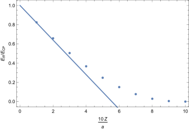
Figure 1: The renormalized TE CP energy for the potential (24), describing the medium bwtween a polarizable atom and a perfectly conducting plate, relative to the vacuum value (9). The dots are the results of numerical integration, while the straight line is the perturbative approximation (26).

The corresponding results for the TM mode are shown in Fig. 2. Note now the perturbative approximation is

$$E^{\rm TM}_{p}=-\frac{5\alpha}{16\pi Z^{4}}\left(1-\frac{97}{45}Z\right).$$ (27)

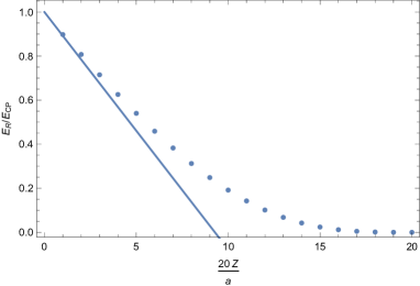
Figure 2: The renormalized TM CP energy for the potential (24), describing the medium between a polarizable atom and a perfectly conducting plate, relative to the vacuum value (12). The dots are the results of numerical integration, while the straight line is the perturbative approximation (27).

Now we illustrate what can happen when the analytically continued permittivity develops a singularity in the extended region. So consider the permittivity

$$\varepsilon(z)=\frac{\lambda}{(a+z)^{2}},$$ (28)

which now has the singularity at $-a$. The solutions are like before, with $(a-z)$ replaced by $(a+z)$ but now we have to interchange the roles of $I_{\nu}$ and $K_{\nu}$ because we want $F$ to vanish at infinity, and $\tilde{G}$ to be well-behaved at $z=-a$. The formula for the renormalized TE energy is then

$$E_{R}^{E}=-\frac{\alpha}{\lambda^{3/2}\pi}(a+Z)\int_{0}^{\infty}dk\,k\int_{1/4}^{\infty}d\nu\,\nu\sqrt{\nu^{2}-1/4}\frac{I_{\nu}(ka)}{K_{\nu}(ka)}K^{2}_{\nu}(k(a+Z)),$$ (29)

where we have changed the integration variable from $\zeta$ to $\nu$. Again we consider the case $\lambda/a^{2}=1$. The perturbative approximation to this is Eq. (26) with the reversed sign of the linear term. The numerical integration is compared with the perturbative approximation in Fig. 3.

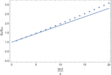
Figure 3: The renormalized TE CP energy for the potential (28), describing the medium between a polarizable atom and a perfectly conducting plate, relative to the vacuum value (9). The dots are the results of numerical integration, while the straight line is the relative perturbative correction $1+\frac{9}{5}Z$. It is seen this is the continuation of the results seen in Fig. 1.

5 Conclusion

We have show how to isolate a finite, “renormalized” Casimir-Polder interaction energy between a plane surface of nonanalyticity, which includes a perfect reflector, and an isotropic polarizable atom, separated by an inhomogeneous dispersive medium. (For simplicity the inhomogeneity is restricted to a single direction, perpendicular to the plane interface.) Incorporation of anisotropy and of dispersion in the polarizability is readily achievable. Elsewhere we will consider the more complicated problem of the Casimir interaction between two such interfaces [14].

Funding

National Science Foundation (NSF) (1707511)

References

- [1] H. B. G. Casimir and D. Polder, “The influence of retardation on the London-van der Waals forces,” \JournalTitlePhys. Rev. 73, 360–372 (1948). doi:10.1103/PhysRev.73.360
- [2] F. London, “Zur Theorie und Systematik der Molekularkräfte,” \JournalTitleZ. Physik, 63, 245–279 (1930).
- [3] C. I. Sukenik, M. G. Boshier, D. Cho, V. Sundoghar, and E. A. Hinds, “Measurement of the Casimir-Polder force,” \JournalTitlePhys. Rev. Lett. 70, 560–563 (1993).
- [4] D. M. Harber, J. M. Obrecht, J. M. McGuirk, and E. A. Cornell, “Measurement of the Casimir-Polder force through center-of-mass oscillations of a Bose-Einstein condensate,” \JournalTitlePhys. Rev. A 72, 033610 (2005).
- [5] E. M. Lifshitz, “The theory of molecular attractive forces between solids,” \JournalTitleZh. Eksp. Teor. Fiz., 29, 94–110 (1955) [English transl.: \JournalTitleSoviet Phys. JETP 2, 73–83 (1956)].
- [6] I. D. Dzyaloshinskii, E. M. Lifshitz, and L. P. Pitaevskii, “General theory of van der Waals forces,” \JournalTitleUsp. Fiz. Nauk 73, 381–422 (1961) [English transl.: \JournalTitleSoviet Phys. Usp. 4, 153–176 (1961); \JournalTitleAdv. Phys.. 10, 165–208 (1961).]
- [7] I. Griniasty and U. Leonhardt, “Casimir stress inside planar materials,” \JournalTitlePhys. Rev. A 96, 032123 (2017).
- [8] I. Griniasty and U. Leonhardt, “Casimir stress in materials: Hard divergency at soft walls,” \JournalTitlePhys. Rev. B 96, 205418 (2017).
- [9] Fanglin Bao, Bin Luo, and Sailing He, “First-order correction to the Casimir force within an inhomogeneous medium,” \JournalTitlePhys. Rev. A 91, 063810 (2015).
- [10] F. Bao, J. S. Evans, M. Fang, and S. He, “Inhomogeneity-related cutoff dependence of the Casimir energy and stress,” \JournalTitlePhys. Rev. A 93, 013824 (2016).
- [11] K. A. Milton, S. A. Fulling, P. Parashar, P. Kalauni and T. Murphy, “Stress tensor for a scalar field in a spatially varying background potential: Divergences, “renormalization,” anomalies, and Casimir forces,” \JournalTitlePhys. Rev. D 93, 085017 (2016) doi:10.1103/PhysRevD.93.085017 [arXiv:1602.00916 [hep-th]].
- [12] S. A. Fulling, T. E. Settlemyre and K. A. Milton, “Renormalization for a scalar field in an external scalar potential,” \JournalTitleSymmetry 10, 54 (2018). doi:10.3390/sym10030054 [arXiv:1802.02883 [hep-th]].
- [13] P. Parashar, K. A. Milton, Y. Li, H. Day, X. Guo, S. A. Fulling and I. Cavero-Peláez, “Quantum electromagnetic stress tensor in an inhomogeneous medium,” \JournalTitlePhys. Rev. D 97, 125009 (2018) doi:10.1103/PhysRevD.97.125009 [arXiv:1804.04045 [hep-th]].
- [14] K. A. Milton, Prachi Parashar, Li Yang, Hannah Day, Xin Guo, S. A. Fulling, I. Cavero-Peláez, and G. Kennedy, “Casimir forces in inhomogeneous media,” paper in preparation.