Cosmological Hydrodynamic Simulations with Suppressed Variance in the Lyman-$\alpha$ Forest Power Spectrum

Abstract

We test a method to reduce unwanted sample variance when predicting Lyman-$\alpha$ (Ly$\alpha$) forest power spectra from cosmological hydrodynamical simulations. Sample variance arises due to sparse sampling of modes on large scales and propagates to small scales through non-linear gravitational evolution. To tackle this, we generate initial conditions in which the density perturbation amplitudes are fixed to the ensemble average power spectrum – and are generated in pairs with exactly opposite phases. We run $50$ such simulations ($25$ pairs) and compare their performance against $50$ standard simulations by measuring the Ly$\alpha$ 1D and 3D power spectra at redshifts $z=2$, 3, and 4. Both ensembles use periodic boxes of $40\ h^{-1}\text{Mpc}$ containing $512^{3}$ particles each of dark matter and gas. As a typical example of improvement, for wavenumbers $k=0.25\ h\text{Mpc}^{-1}$ at $z=3$, we find estimates of the 1D and 3D power spectra converge $34$ and $12$ times faster in a paired-fixed ensemble compared with a standard ensemble. We conclude that, by reducing the computational time required to achieve fixed accuracy on predicted power spectra, the method frees up resources for exploration of varying thermal and cosmological parameters – ultimately allowing the improved precision and accuracy of statistical inference.

1 Introduction

Precision cosmology with the Lyman-$\alpha$ forest is an area of increasing interest, both for its ability to constrain the evolution of the Universe (McDonald & Eisenstein, 2007; Busca et al., 2013; Slosar et al., 2013; Font-Ribera et al., 2014; Bautista et al., 2017; du Mas des Bourboux et al., 2017) and for its unique insight into the small-scale power spectrum that is a potential diagnostic of warm dark matter, neutrinos, and other particle physics phenomena (Seljak et al., 2005, 2006a, 2006b; Viel et al., 2006, 2013a; Palanque-Delabrouille et al., 2015; Iršič et al., 2017). For the latter studies it is essential to explore the effect of both particle physics and astrophysical parameters on the measured power spectrum, since there are important degeneracies with the thermal and ionization history of the intergalactic medium (IGM) that need to be considered (McDonald et al., 2005a; McQuinn, 2016; Walther et al., 2018).

Ideally one runs a series of cosmological simulations to forward model the parameters into mock observables that can be compared with data (McDonald et al., 2005b; Viel & Haehnelt, 2006; Borde et al., 2014). However, the mock observations suffer from intrinsic sample variance due to the finite simulation box size; sparse sampling of random phases and amplitudes of large-scale modes in the initial conditions propagate to an uncertainty in the final mock power spectrum. This uncertainty can affect even small-scale modes through non-linear gravitational coupling. In practice, model uncertainty is the limiting factor on large scales where it exceeds the observational uncertainty (Palanque-Delabrouille et al., 2015) Suppressing the uncertainties can be achieved either by expanding the box size, or by averaging many simulated realizations of the same volume size; either way a more precise mean power spectrum (or other observable) can be achieved. But each simulation is expensive, especially as the box size is increased. To extract the best possible constraints, one has to tension this need for large sample sizes or volumes for a single point in parameter space against the requirement to adequately sample the parameter space itself.

This paper examines an approach to lessen the tension, by initializing simulations with carefully chosen amplitudes and phases for each mode, thus reducing the total volume or number of simulations required to achieve a given statistical accuracy on the mean mock power spectrum. This approach will free up computing time per parameter instantiation to increase the density of samples in parameter space. Methods, such as emulators (Bird et al. in prep.; Rogers et al. in prep.), which interpolate between hydrodynamic simulations predictions, can then be more accurate. Interpolation is necessary because only a limited number of simulations can feasibly be run.

We minimize the number of simulation realizations by running paired, fixed simulations (Pontzen et al., 2016; Angulo & Pontzen, 2016). The difference between the standard simulations and the paired-fixed simulations is in the input density field. For a Gaussian random field, the amplitude of each mode is drawn from a Rayleigh distribution with zero mean and variance equal to the power spectrum at that scale, and the phase drawn with uniform probability between 0 and $2\pi$. Instead, for paired-fixed simulations, we fix the amplitudes of the Fourier modes to the square root of the power spectrum, and invert the phase of one simulation in a pair relative to the other. The fixing reduces the variance of the power spectrum on the largest scales, which remain in or near the linear regime, while the pairing cancels leading-order errors due to non-linear evolution of chance correlations between large-scale modes.

On its own pairing is a benign manipulation in the sense that both realisations in the pair are legitimate, equally-likely draws from a Gaussian random field (Pontzen et al., 2016). Fixing, on the other hand, generates an ensemble that is quantitatively different from Gaussian; Angulo & Pontzen (2016) argued that, to any order in perturbation theory, the differences affect only the variance on the power spectrum and cannot propagate to other observables such as the power spectrum or observable measures of non-Gaussianity. Combined, pairing and fixing thus formally removes the leading order and next-to-leading order uncertainties that generate scatter in predicted mock observations from simulations. In Villaescusa-Navarro et al. (2018), we thoroughly explored the statistics of paired-fixed simulations for both dark matter evolution and galaxy formation, finding that there are no statistically significant biases in the approach, and in many settings it does yield significantly enhanced statistical accuracy.

In this paper, we apply these techniques for the first time to the study of the power spectrum of fluctuations in the Lyman-$\alpha$ (Ly$\alpha$) forest, as measured from hydrodynamical simulations. The Ly$\alpha$ forest is the collection of absorption features present in distant quasar spectra due to intervening neutral hydrogen absorbing Ly$\alpha$ photons as the quasar light redshifts. Physically, the forest comprises a relatively smooth, low density environment of hydrogen which traces the underlying matter density of the Universe well in the redshift range $2<z<5$ (Croft et al., 1998; Hernquist et al., 1996). At higher redshifts $z>5$ and especially beyond reionization the neutral hydrogen is too optically thick (Gunn & Peterson, 1965); at lower redshift $z<2$ the forest cannot be observed with optical instruments. Although use of the Ly$\alpha$ forest as a tracer of the matter density is limited to a finite redshift interval, it is a unique probe of a wide range of otherwise inaccessible redshifts and scales. It has the unique advantage of tracing the matter density at small scales, down to 10s of kpc, in regions where the evolution is still close to linear.

This paper is structured as follows. In Section 2 we describe the simulations used in this analysis, before presenting results in Section 3. We conclude in Section 4 with a brief summary and discussion.

2 Simulations

In this section we describe the simulations used in this study. We start by describing the different sets of initial conditions (Gaussian, fixed and paired-fixed); we will then discuss the hydrodynamical simulations and the method to simulate Ly$\alpha$ forest sightlines from the simulations.

2.1 Gaussian, Fixed and Paired-Fixed Random Fields

In this paper we will follow the naming convention in Villaescusa-Navarro et al. (2018), which contains more detailed definitions including power spectrum conventions. Here we present a brief summary of the required definitions to interpret our results.

Given a density field $\rho(\vec{x})$, the density contrast is defined as

$$\delta(\vec{x})=\frac{\rho(\vec{x})-\bar{\rho}}{\bar{\rho}}~{},$$ (1)

where $\bar{\rho}=\langle\rho(\vec{x})\rangle$. In a simulation we take discretized values of these quantities at the center of a cell $\vec{x_{i}}$, $\delta_{i}=\delta(\vec{x_{i}})$, and define discrete Fourier modes $\tilde{\delta}_{n}$ as

$$\tilde{\delta}_{n}=\sum_{i}\delta_{i}~{}e^{i\vec{x}_{i}\cdot\vec{k}_{n}}=A_{n}~{}e^{i\theta_{n}}~{},$$ (2)

where $\vec{k}_{n}$ identifies the wavenumber, $A_{n}$ is the amplitude of the discrete Fourier mode and $\theta_{n}$ is the phase.

For a Gaussian density field, each $\theta_{n}$ is a random variable distributed uniformly between 0 and $2\pi$ and each $A_{n}$ follows a Rayleigh distribution

$$p(A_{n})~{}{\rm d}A_{n}=\frac{A_{n}}{\sigma_{n}^{2}}~{}e^{-A_{n}^{2}/2\sigma_{n}^{2}}{\rm d}A_{n}~{},$$ (3)

with $\langle A_{n}\rangle=\sqrt{\frac{\pi}{2}}~{}\sigma_{n}$, and $\sigma_{n}^{2}$ is proportional to the power spectrum $P(|\vec{k}_{n}|)$ (with the constant of proportionality depending on the particular conventions adopted; see Villaescusa-Navarro et al. (2018)).

For generating initial conditions (ICs) representing a discretized Gaussian density field for a simulation of the Universe, the mode amplitudes ($A_{n}$) and phases ($\theta_{n}$) are chosen randomly from their distributions above. This randomness generates a source of variance in the final mock power spectrum from the simulation; the amplitudes $A_{n}$ propagate directly, while the phases $\theta_{n}$ become significant during non-linear evolution because their values determine how modes of different scales interact with each other.

In this paper, we explore alternative approaches to generating ICs such that these variance effects are minimised. Similar to Villaescusa-Navarro et al., we define Gaussian, paired Gaussian, fixed and paired-fixed fields as follows:

• Gaussian field: A field with $\tilde{\delta}_{n}=A_{n}~{}e^{i\theta_{n}}$, where $A_{n}$ follows the Rayleigh distribution of Eq. 3 and $\theta_{n}$ is a random variable distributed uniformly between 0 and $2\pi$.

• Paired Gaussian field: A pair of Gaussian fields $\delta$ and $\delta^{\prime}$, where $\tilde{\delta}_{n}=A_{n}~{}e^{i\theta_{n}}$ and $\tilde{\delta}_{n}^{\prime}=A_{n}~{}e^{i(\theta_{n}+\pi)}=-\tilde{\delta}_{n}$; the values of $A_{n}$ and $\theta_{n}$ are the same for the two fields and $A_{n}$ is drawn from the Rayleigh distribution of Eq. 3. Because the leading-order uncertainties are typically from the amplitudes rather than the phases, we do not use paired fields without fixing the amplitudes in this work.

• Fixed field: A field with $\tilde{\delta}_{n}=A_{n}~{}e^{i\theta_{n}}$, where we fix $A_{n}=\sqrt{2}~{}\sigma_{n}$. The phase $\theta_{n}$ remains a uniform random variable between $0$ and $2\pi$.

• Paired-fixed field: A pair of fields, $\tilde{\delta}_{n}=A_{n}~{}e^{i\theta_{n}}$ and $\tilde{\delta}_{n}^{\prime}=A_{n}~{}e^{i(\theta_{n}+\pi)}=-\tilde{\delta}_{n}$, where the values of $A_{n}$ are the same for the two fields and fixed to $A_{n}=\sqrt{2}~{}\sigma_{n}$, and the values of $\theta_{n}$ are also the same for the two fields, as defined, rendering $\tilde{\delta}_{n}$ and $\tilde{\delta}_{n}^{\prime}$ exactly out of phase with respect to each other. Here $\theta_{n}$ remains a uniform random variable between $0$ and $2\pi$.

The purpose of this paper is to compare the statistical accuracy of paired-fixed simulations with standard simulations (based on Gaussian fields), in the context of Ly$\alpha$ forest power spectrum analyses.

2.2 Hydrodynamical simulations

We perform hydrodynamical simulations with the Gadget-3 code, a modified version of the publicly available code Gadget-2 (Springel, 2005). The code incorporates radiative cooling by primordial hydrogen and helium, alongside heating by the UV background following the model of Viel et al. (2013b). The quick-lya flag is enabled, so gas particles with overdensities larger than 1000 and temperatures below $10^{5}$ K are converted into collisionless particles (Viel et al., 2004). This approach focuses the computational effort on low-density gas associated with the Ly$\alpha$ forest, and is much more efficient than either allowing dense gas to accumulate or adopting a realistic galaxy formation and feedback model, to which the forest is largely insensitive. Thus, this computational efficiency has no significant effect on the accuracy of estimated Ly$\alpha$ forest observables.

The initial conditions are generated at $z=99$ by displacing cold dark matter (CDM) and gas particles from their initial positions in a regular grid, according to the Zel’dovich approximation. We account for the different power spectra and growth factors of CDM and baryons by rescaling the $z=0$ linear results according to the procedure described in Zennaro et al. (2017).

Our simulations evolve $512^{3}$ CDM and $512^{3}$ gas particles from $z=99$ down to $z=2$ within a periodic box of $40\ h^{-1}\text{Mpc}$, storing snapshots at redshifts 4, 3 and 2. We run a total of 100 simulations (25 fixed pairs, and 50 standard simulations). In order to study the dependence of our results on volume we also run an identical set of simulations as those described above but with $256^{3}$ CDM and $256^{3}$ gas particles in a box of size $20\ h^{-1}\text{Mpc}$.

The values of the cosmological parameters, the same for all simulations, are in good agreement with results from Planck Collaboration et al. (2016): $\Omega_{\rm m}=0.3175$, $\Omega_{\rm b}=0.049$, $\Omega_{\nu}=0$, $\Omega_{\Lambda}=0.6825$, $h=0.67$, $n_{s}=0.9624$, $\sigma_{8}=0.834$.

2.3 Modeling Ly$\alpha$ absorption

In order to study Ly$\alpha$ forest flux statistics we generate a set of mock spectra containing only the Ly$\alpha$ absorption line from neutral hydrogen for each snapshot in our simulation suite. The spectra are calculated on a square grid of 160 000 spectra for the 40 Mpc box. Each spectrum extends the full length of the box, and maintains the periodic boundary conditions of the underlying simulation, with sizes in velocity space of $[3\,793,4\,267,4\,698]\,\mathrm{km}\,\mathrm{s}^{-1}$ respectively at $z=[2,3,4]$. In each spectrum, the optical depth $\tau$ is calculated by taking the product of the column density of neutral hydrogen and the atomic absorption coefficient for the Ly$\alpha$ line (Humlicek, 1979) appropriately redshifted for both its cosmological and peculiar velocities. Measurements are made in bins of velocity width $10\,\mathrm{km}\,\mathrm{s}^{-1}$ using the code fake_spectra (Bird, 2017).

Once we have computed the Ly$\alpha$ optical depth, we derive the transmitted flux fraction (or flux for short):

$$F=e^{-\tau}~{}.$$ (4)

We then calculate $\bar{F}$, the mean flux over all pixels in our box. Next, we adopt the common practice of rescaling the optical depth of each simulation, $\tau\to\alpha\tau$ where $\alpha$ is chosen to fix $\bar{F}$ to a target value. This is normally adopted when making comparisons to data because it reduces the impact of uncertainties in the UV background. In our case, we set $\alpha$ in each simulation such that $\bar{F}$ is fixed to the mean over all simulations. We verified that, if we do not renormalize $\tau$, the benefits of paired and fixed simulations remain (in fact they even increase further on small scales). After renormalization, we calculate the fluctuations around the mean, $\delta_{F}$:

$$\delta_{F}=\frac{F}{\bar{F}}-1~{}.$$ (5)

Finally, we calculate flux power spectra using the code lyman_alpha (Rogers et al., 2018a, b). Studies of the Ly$\alpha$ forest either adopt 1D or 3D power spectra depending on the density of available observational skewers; the former approach is computationally simpler and captures small-scale line-of-sight information, while the latter approach is required to capture larger-scale correlations that do not fit within a single quasar spectrum. In this work we will study the effects of paired-fixed simulations in both settings.

To create a mock power spectrum, the first step is to generate the Fourier transform ($\tilde{\delta}_{F}$) of the fluctuation field $\delta_{F}$. For 1D power spectra, the transformation is taken separately for each skewer along the line-of-sight direction; otherwise we apply the 3D transformation to the entire box. In both cases we are able to exploit fast Fourier transforms since all velocity bins are of equal width and spectra are evenly sampled in the transverse direction. We then estimate power spectra by averaging $|\tilde{\delta}_{F}|^{2}$ over all skewers for the 1D power spectrum, or in $|\vec{k}|$ shells for the 3D power spectrum.

When working with paired simulations, we average the power spectra to form a single estimate from each pair. This leaves us with $25$ independent estimates from our ensemble of $50$ paired-fixed simulations, a point that will be discussed further below.

3 Results

In this Section we will present the statistical performance of our different simulations in predicting Ly$\alpha$ power spectra. To quantify the performance of any given ensemble, we calculate the mean of the measured power across all realizations, $\bar{P}(k)$

$$\bar{P}(k)=\frac{1}{N_{\mathrm{est}}}\sum_{i=1}^{N_{\mathrm{est}}}P_{i}(k)\,,$$ (6)

where $N_{\mathrm{est}}$ is the number of independent estimates of $\bar{P}(k)$ and $P_{i}(k)$ are the individual estimates. We also calculate the single-estimate variance in $P(k)$:

$$\sigma^{2}(P(k))=\frac{1}{N_{\mathrm{est}}-1}\sum_{i=1}^{N_{\mathrm{est}}}\left(P_{i}(k)-\bar{P}(k)\right)^{2}\,,$$ (7)

As noted above, in the case of paired (or paired-fixed) simulations $N_{\mathrm{est}}=N_{\mathrm{sim}}/2$, while in the case of a standard ensemble, $N_{\mathrm{est}}=N_{\mathrm{sim}}$ where in both cases $N_{\mathrm{sim}}=50$, the number of simulations. This difference arises because paired power spectrum estimates are not independent and instead the average of each pair is regarded as providing a single sample $P_{i}(k)$.

We are actually interested in the expected uncertainty on the mean power spectrum, $(\Delta\bar{P})^{2}$, estimated as

$$(\Delta\bar{P})^{2}\equiv\frac{\sigma^{2}(P(k))}{N_{\mathrm{est}}}\textrm{.}$$ (8)

The ratio of the standard to the paired-fixed uncertainties gives the most useful performance metric; in our case where $N_{\mathrm{sim}}$ is the same between the two ensembles, this reduces to

$$\frac{(\Delta\bar{P}_{\mathrm{S}})^{2}}{(\Delta\bar{P}_{\mathrm{PF}})^{2}}=\frac{\sigma^{2}_{\mathrm{S}}(P(k))}{2\sigma^{2}_{\mathrm{PF}}(P(k))}\,,$$ (9)

where S and PF subscripts refer to the standard (Gaussian) and paired-fixed ensembles respectively. This ratio can also be thought of as the computational speed-up for achieving a fixed target accuracy (assuming the uncertainty on the mean power spectrum scales proportional to $\sqrt{N_{\mathrm{sim}}}$). It limits to unity when the paired-fixed approach is not providing any improvement.

From our paired-fixed simulations we can also form a fixed ensemble simply by discarding one of each pair. Thus we will also show results for a fixed ensemble with $N_{\mathrm{est}}=N_{\mathrm{sim}}=25$. Once again the estimated accuracy of the mean power is given by Equation (9), including the factor $2$ renormalisation for the relative number of estimates.

To ensure that the manipulations of the initial conditions do not introduce any bias, we also calculate $\bar{P}_{\mathrm{S}}-\bar{P}_{\mathrm{PF}}$. For finite $N_{\mathrm{sim}}$ this difference contains a residual statistical uncertainty; one should expect

$$\langle(\bar{P}_{\mathrm{S}}-\bar{P}_{\mathrm{PF}})^{2}\rangle=(\Delta\bar{P}_{\mathrm{S}})^{2}+(\Delta\bar{P}_{\mathrm{PF}})^{2}\,,$$ (10)

given the independence of the two ensembles. Therefore we check that $\bar{P}_{\mathrm{S}}-\bar{P}_{\mathrm{PF}}$ remains comparable in magnitude to this expected residual.

3.1 Matter Power Spectrum

We start by discussing the matter power spectrum (i.e. the 3D power spectrum of the overdensity field without any transformation to Ly$\alpha$ flux); Villaescusa-Navarro et al. (2018) also discussed this quantity, but not at the redshifts in which we are interested in this work. Our simulations also have different baryonic physics implementations.

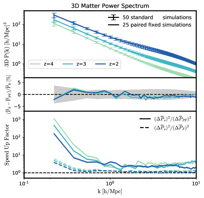
Figure 1: Matter power spectrum measured at $z=2,3$ and $4$. The top panel shows the mean power spectrum in the two sets of simulations, the standard simulations, $\bar{P}_{\rm S}$, with the $1\sigma$ uncertainty on the mean, and the paired-fixed simulations, $\bar{P}_{\rm PF}$; the means are indistinguishable. The middle panel shows the fractional difference between the mean power measured in the two sets of simulations, with a shaded region showing the expected $1\sigma$ uncertainty on that difference which is given by Eq. 10. Across all scales, there is no evidence for bias in the estimate of the paired-fixed simulations relative to the traditional simulations. The bottom panel shows the ratio between the uncertainty on the mean of the standard and paired-fixed simulations, $(\Delta\bar{P}_{\mathrm{S}})^{2}/(\Delta\bar{P}_{\mathrm{PF}})^{2}$, with dashed lines showing instead the effect of fixing without pairs $(\Delta\bar{P}_{\mathrm{S}})^{2}/(\Delta\bar{P}_{\mathrm{F}})^{2}$. These ratios summarise how fast the paired-fixed (or fixed) simulations converge on the mean power spectrum relative to the standard simulations. As a typical example of improvement, for wavenumbers $k=0.25\ h\text{Mpc}^{-1}$ and $2\ h\text{Mpc}^{-1}$ at $z=3$, we find estimates of the matter power spectra converge $390$ and $2.0$ times faster in the paired-fixed simulations compared with the standard simulations.

In Figure 1 we show the matter power spectrum measured at $z=2,3,\mathrm{and}\;4$. In the top panel we show the average power spectrum in the two ensembles: the set of 50 standard simulations $\bar{P}_{\rm S}$ and the set of 25 paired-fixed simulations $\bar{P}_{\rm PF}$. Error bars show the uncertainties $\Delta\bar{P}_{\rm S}$ in the mean of the standard simulations, computed using Equation (8). The uncertainties are small due to the large number of simulations. The uncertainties in the paired-fixed simulation are too small to be plotted in the top panel, as we will shortly discuss.

The middle panel shows the difference between the mean power measured in the two sets of simulations, as a fraction of the total power in the standard simulations. Additionally we show, as a grey band, the $\pm 1\sigma$ uncertainty at $z=3$ defined by Equation (10). The two approaches to estimating the non-linear power spectrum thus agree well, consistent with Angulo & Pontzen (2016) and Villaescusa-Navarro et al. (2018). In the bottom panel we quantify the statistical improvement achieved by the paired-fixed simulations with respect to the standard simulations. We show the ratios of the uncertainty on the means, comparing the standard and paired-fixed simulations, $(\Delta\bar{P}_{\rm S})^{2}/(\Delta\bar{P}_{\rm PF})^{2}$, Equation (9). This ratio represents how quickly the paired-fixed simulations converge on the true mean relative to the standard simulations. We also show the ratio of the uncertainty on the means of the standard simulations and fixed (but not paired) simulations, shown as the dashed lines. The dotted horizontal line shows a value of 1, indicating the level where fixed and paired-fixed simulations do not bring any statistical improvement over standard simulations. Comparing the solid and dashed lines shows that both fixing and pairing the simulations contributes to reducing uncertainty on the mean power spectrum at low $k$. As a typical example of improvement, for wavenumbers $k=0.25\ h\text{Mpc}^{-1}$ and $2\ h\text{Mpc}^{-1}$ at $z=3$, we find estimates of the matter power spectra converge $390$ and $2$ times faster in paired-fixed simulations compared with standard simulations.

Broadly this agrees with results from Villaescusa-Navarro et al. (2018) but, unlike in the earlier work, we find that the factor $\simeq 2$ improvement in a paired-fixed simulation continues to $k=10\ h\text{Mpc}^{-1}$. To isolate the cause of this difference, we first considered the effect of box size. Our simulations are of boxes with side length $40\ h\text{Mpc}^{-1}$, which is intermediate between boxes considered by Villaescusa-Navarro et al. (2018). We therefore ran a suite of smaller $20\ h\text{Mpc}^{-1}$ simulations for direct comparison to the smallest boxes of that earlier work. However we found similar results at large $k$ in this additional suite, and conclude that box size is not the driver for the different behavior. The only remaining difference between our present simulations and the hydrodynamic simulations of Villaescusa-Navarro et al. (2018) lies in the drastically different baryonic physics implementation. As discussed in Section 2.2, we do not implement feedback but instead use an efficient prescription to convert high density gas into collisionless particles. By contrast, Villaescusa-Navarro et al. (2018) adopts a state-of-the-art star formation and feedback prescription which results in significant mass transport due to galactic outflows. We verified that the $20\ h^{-1}\text{Mpc}$ dark-matter-only runs of Villaescusa-Navarro et al. (2018), like our Ly$\alpha$ runs, also generate substantial improvements from pairing and fixing at high $k$. It therefore seems that potential efficiency gains at $k\gg 1\ h\text{Mpc}^{-1}$ can be erased by stochastic noise from sufficiently energetic feedback and winds.

Our practical conclusions will be insensitive to this regime. Uncertainties at high $k$ are dominated by observational rather than theoretical uncertainty, due to the rapidly shrinking absolute magnitude of simulation sample variance. Because the sample variance is intrinsically small, it is only important that the power spectrum remains unbiased at these scales.

3.2 3D Ly$\alpha$ Power Spectrum

We next turn our attention to the 3D Ly$\alpha$ power spectrum. On large, quasi-linear scales, the 3D Ly$\alpha$ power spectrum is proportional to the matter power spectrum, with an amplitude set by the scale-independent bias parameter, and an angular dependence described by the Kaiser (1987) model of linear redshift-space distortions. In this work, we include these distortions but consider the angle-averaged (i.e. monopole) power spectrum rather than divide the power spectrum into angular bins.

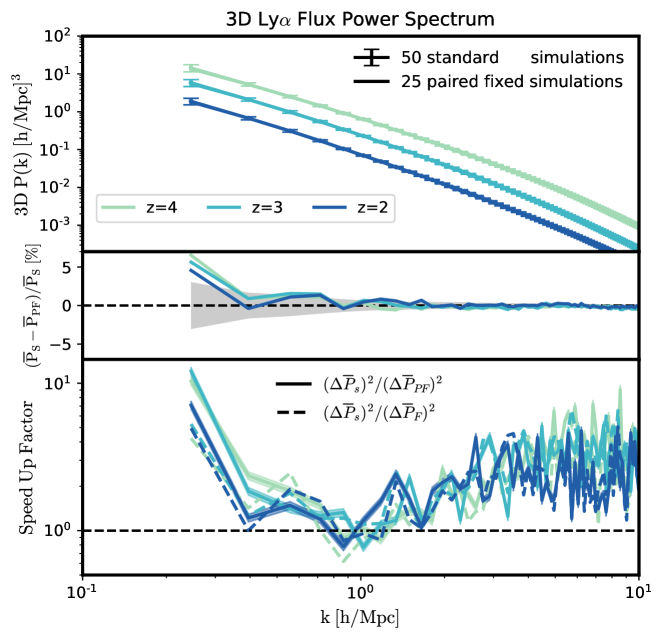
Figure 2: Same as Figure 1, but for the 3D Ly$\alpha$ flux power spectrum. As a typical example of improvement, for wavenumbers $k=0.25\ h\text{Mpc}^{-1}$ and $2\ h\text{Mpc}^{-1}$ at $z=3$, we find estimates of the 3D Ly$\alpha$ flux power spectra converge $12$ and $2.0$ times faster in a paired-fixed ensemble compared with a standard ensemble.

We present the measured 3D Ly$\alpha$ forest power spectrum in Figure 2. The panels are computed and arranged as in Figure 1, but starting from the flux $\delta_{F}$ instead of the overdensity $\delta$. In the top panel the uncertainties on the mean power spectrum of the standard simulations are again small due to the large number of simulations. The middle panel shows the fractional difference between the paired-fixed and standard simulation power spectra, with the grey shaded region again indicating the expected $1\sigma$ scatter. Several measured points scatter outside this envelope (most notably at $k<0.3\ h\text{Mpc}^{-1}$) but this is consistent with a statistical fluctuation driven by scatter in the standard ensemble. At high $k$ the difference in the mean is sub-percent. Comparing the central panels of Figures 1 and 2 reveals that the shape of the $1\sigma$ contour is different between the Ly$\alpha$ and matter power cases. At high $k$, the matter power enters a highly non-linear regime where modes are strongly coupled, whereas the flux arises from low density clouds that are still quasi-linear. In the case of flux, modes are near-decoupled and the uncertainty decays proportionally to the increasing number of modes per $k$ shell.

The bottom panel of Figure 2 quantifies the statistical improvement achieved by the paired-fixed simulations with respect to the standard simulations, shown as the solid line. The dashed line represents simulations that are just fixed. The dotted horizontal line shows a value of 1, indicating the level where fixed and paired-fixed simulations do not bring any statistical improvement over standard simulations. As a typical example of improvement, for wavenumbers $k=0.25\ h\text{Mpc}^{-1}$ and $2\ h\text{Mpc}^{-1}$ at $z=3$, we find estimates of the 3D Ly$\alpha$ flux power spectra converge $12$ and $2$ times faster in a paired-fixed ensemble compared with a standard ensemble.

There is a minimum level of improvement at $k\simeq 1\ h\text{Mpc}^{-1}$ where the paired-fixed approach does not outperform the standard ensemble at $z=3$. The relative performance improvements then increases with increasing $k$ beyond this point, which is surprising. Previously it has been argued that the improvements generated by the paired-fixed approach can be understood within the framework of standard perturbation theory (Angulo & Pontzen, 2016; Pontzen et al., 2016) which more obviously applies to intermediate quasi-linear scales than the $k>1\ h\text{Mpc}^{-1}$ regime.

At present we cannot fully explain why pairing and fixing improves the Ly$\alpha$ power spectrum accuracy in this regime. It might be that super-sample covariance terms couple high $k$ to low $k$ in a unique way given that the forest is dominated by underdense regions (unlike the matter power spectrum; Takada & Hu, 2013). However, we did not investigate further for this work because the improvements are not particularly relevant for observational studies; the absolute magnitude of the model uncertainties in the $k>1\ h\text{Mpc}^{-1}$ rapidly become smaller than observational uncertainties (see top panel of Figure 2 for a visualization of the magnitude of the model uncertainties). Thus the improvements in accuracy at low $k$ are of most practical benefit to future work.

3.3 1D Ly$\alpha$ Power Spectrum

Most hydrodynamical simulations of the Ly$\alpha$ forest have been used to predict the 1D power spectrum (McDonald et al., 2005b; Viel & Haehnelt, 2006; Borde et al., 2014; Lukić et al., 2015; Walther et al., 2018). As described in Section 2.3, the 1D spectrum captures small-scale information along the line of sight without the computational complexity of cross-correlating between different skewers.

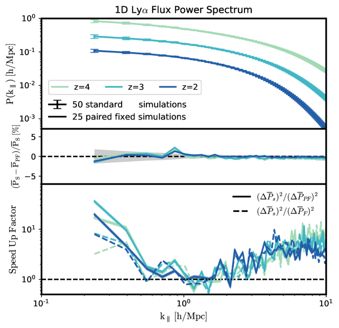
Figure 3: Same as Figure 1, but for the 1D Ly$\alpha$ flux power spectrum. The line-of-sight wavenumber $k_{\parallel}$ corresponds to an integral over many 3D wavenumbers $k$, so there is not a direct correspondence between the scales. As a typical example of improvement, for wavenumbers $k_{\parallel}=0.25\ h\text{Mpc}^{-1}$ and $2\ h\text{Mpc}^{-1}$ at $z=3$, we find estimates of the 1D Ly$\alpha$ flux power spectra converge $34$ and $1.7$ times faster in a paired-fixed ensemble compared with a standard ensemble.

We present the measured 1D Ly$\alpha$ power spectrum in Figure 3, using again the same panel layout as Figure 1. In the top panel the uncertainties on the mean power spectrum of the standard simulations are, as usual, small due to the large number of simulations. The middle panel shows the fractional uncertainty in the paired-fixed simulations relative to the standard simulations, with the grey shaded region indicating the $1\sigma$ uncertainty on this difference. Once again there is overall good agreement, with the strongest deviation arising at $k=0.9\ h\text{Mpc}^{-1}$ at a significance of almost $2\sigma$. However the difference between our standard and paired-fixed ensemble remains less than $2\%$, and (given the large number of independent $k$ bins) we believe the difference to be consistent with the expected level of statistical fluctuations.

The bottom panel quantifies the statistical improvement achieved by the paired-fixed simulations (solid line) with respect to the standard simulations. The dashed line represents simulations that are fixed but not paired. As a typical example of improvement, for wavenumbers $k_{\parallel}=0.25\ h\text{Mpc}^{-1}$ and $2\ h\text{Mpc}^{-1}$ at $z=3$, we find estimates of the 1D Ly$\alpha$ flux power spectra converge $34$ and $1.7$ times faster in a paired-fixed ensemble compared with a standard ensemble. As with the 3D Ly$\alpha$ flux power (Section 3.2) there is a steadily increasing improvement at high $k$, forming a local minimum at $k_{\parallel}\simeq 1\ h\text{Mpc}^{-1}$; since the 1D power spectrum mixes multiple modes from the 3D power spectrum, this is consistent with projecting the improvement discussed in Section 3.2.

4 Discussion and Conclusions

We have shown that using the method of paired-fixed simulations reduces the uncertainty of the mean mock Ly$\alpha$ forest power spectrum measured in hydrodynamical simulations, and therefore requires less computing time to estimate the expected value of the considered quantity, which is needed to evaluate the likelihood of the data. As a typical example of improvement, for wavenumbers $k=0.25\ h\text{Mpc}^{-1}$ at $z=3$, we find estimates of the 1D and 3D power spectra converge $34$ and $12$ times faster in a paired-fixed ensemble compared with a standard ensemble. The largest improvements are at small k, where model uncertainties are larger than observational uncertainties. The improvements are minimal at $k=1\ h\text{Mpc}^{-1}$, but at these scales the observational uncertainties are larger than the model uncertainties, so reduced uncertainty on the mean mock power spectrum is unnecessary. This suggests that running a large simulation box size with paired-fixed ICs will provide the most accurate mock Ly$\alpha$ forest power spectrum over the largest range of scales.

By reducing the computational time required to achieve a target accuracy for mock power spectra, the method frees up resources for a more thorough exploration of astrophysical and cosmological parameters. It is essential to be able to sample efficiently over this space, with at least three parameters describing the shape and amplitude of the input linear power spectrum and at least two for astrophysical effects to span the reionisation redshift and level of heat injection. In future, likelihoods for datasets such as eBOSS and DESI will likely take advantage of emulators which interpolate predicted power spectra within these high-dimensional parameter spaces (Heitmann et al. (2016); Walther et al. (2018), Rogers et al in prep, Bird et al in prep). In this context, freeing up CPU time by using the paired-fixed approach will allow for a denser sampling of training points for the emulator. That in turn will beat down interpolation errors and thus lead to more accurate inferences from forthcoming data.

References

- Angulo & Pontzen (2016) Angulo, R. E., & Pontzen, A. 2016, MNRAS, 462, L1
- Astropy Collaboration et al. (2013) Astropy Collaboration, Robitaille, T. P., Tollerud, E. J., et al. 2013, A&A, 558, A33
- Bautista et al. (2017) Bautista, J. E., Busca, N. G., Guy, J., et al. 2017, A&A, 603, A12
- Bird (2017) Bird, S. 2017, FSFE: Fake Spectra Flux Extractor, Astrophysics Source Code Library, , , ascl:1710.012
- Borde et al. (2014) Borde, A., Palanque-Delabrouille, N., Rossi, G., et al. 2014, J. Cosmology Astropart. Phys, 7, 005
- Busca et al. (2013) Busca, N. G., Delubac, T., Rich, J., et al. 2013, A&A, 552, A96
- Croft et al. (1998) Croft, R. A. C., Weinberg, D. H., Katz, N., & Hernquist, L. 1998, ApJ, 495, 44
- du Mas des Bourboux et al. (2017) du Mas des Bourboux, H., Le Goff, J.-M., Blomqvist, M., et al. 2017, A&A, 608, A130
- Font-Ribera et al. (2014) Font-Ribera, A., Kirkby, D., Busca, N., et al. 2014, J. Cosmology Astropart. Phys, 5, 27
- Gunn & Peterson (1965) Gunn, J. E., & Peterson, B. A. 1965, ApJ, 142, 1633
- Heitmann et al. (2016) Heitmann, K., Bingham, D., Lawrence, E., et al. 2016, ApJ, 820, 108
- Hernquist et al. (1996) Hernquist, L., Katz, N., Weinberg, D. H., & Miralda-Escudé, J. 1996, ApJ, 457, L51
- Humlicek (1979) Humlicek, J. 1979, Journal of Quantitative Spectroscopy and Radiative Transfer, 21, 309 . http://www.sciencedirect.com/science/article/pii/0022407379900621
- Hunter (2007) Hunter, J. D. 2007, Computing In Science & Engineering, 9, 90
- Iršič et al. (2017) Iršič, V., Viel, M., Berg, T. A. M., et al. 2017, MNRAS, 466, 4332
- Jones et al. (2001–) Jones, E., Oliphant, T., Peterson, P., et al. 2001–, SciPy: Open source scientific tools for Python, , , [Online; accessed ¡today¿]. http://www.scipy.org/
- Kaiser (1987) Kaiser, N. 1987, MNRAS, 227, 1
- Lukić et al. (2015) Lukić, Z., Stark, C. W., Nugent, P., et al. 2015, MNRAS, 446, 3697
- McDonald & Eisenstein (2007) McDonald, P., & Eisenstein, D. J. 2007, Phys. Rev. D, 76, 063009
- McDonald et al. (2005a) McDonald, P., Seljak, U., Cen, R., Bode, P., & Ostriker, J. P. 2005a, MNRAS, 360, 1471
- McDonald et al. (2005b) McDonald, P., Seljak, U., Cen, R., et al. 2005b, ApJ, 635, 761
- McQuinn (2016) McQuinn, M. 2016, ARA&A, 54, 313
- Palanque-Delabrouille et al. (2015) Palanque-Delabrouille, N., Yèche, C., Lesgourgues, J., et al. 2015, J. Cosmology Astropart. Phys, 2, 45
- Planck Collaboration et al. (2016) Planck Collaboration, Ade, P. A. R., Aghanim, N., et al. 2016, A&A, 594, A13
- Pontzen et al. (2016) Pontzen, A., Slosar, A., Roth, N., & Peiris, H. V. 2016, Phys. Rev. D, 93, 103519
- Rogers et al. (2018a) Rogers, K. K., Bird, S., Peiris, H. V., et al. 2018a, MNRAS, 474, 3032
- Rogers et al. (2018b) —. 2018b, MNRAS, 476, 3716
- Seljak et al. (2006a) Seljak, U., Makarov, A., McDonald, P., & Trac, H. 2006a, Physical Review Letters, 97, 191303
- Seljak et al. (2006b) Seljak, U., Slosar, A., & McDonald, P. 2006b, Journal of Cosmology and Astro-Particle Physics, 10, 14
- Seljak et al. (2005) Seljak, U., Makarov, A., McDonald, P., et al. 2005, Phys. Rev. D, 71, 103515
- Slosar et al. (2013) Slosar, A., Iršič, V., Kirkby, D., et al. 2013, J. Cosmology Astropart. Phys, 4, 26
- Springel (2005) Springel, V. 2005, MNRAS, 364, 1105
- Takada & Hu (2013) Takada, M., & Hu, W. 2013, Phys. Rev. D, 87, 123504
- Van der Walt et al. (2011) Van der Walt, S., Colbert, S. C., & Varoquaux, G. 2011, Computing in Science & Engineering, 13, 22. http://scitation.aip.org/content/aip/journal/cise/13/2/10.1109/MCSE.2011.37
- Viel et al. (2013a) Viel, M., Becker, G. D., Bolton, J. S., & Haehnelt, M. G. 2013a, Phys. Rev. D, 88, 043502
- Viel et al. (2013b) —. 2013b, Phys. Rev. D, 88, 043502
- Viel & Haehnelt (2006) Viel, M., & Haehnelt, M. G. 2006, MNRAS, 365, 231
- Viel et al. (2006) Viel, M., Haehnelt, M. G., & Lewis, A. 2006, MNRAS, 370, L51
- Viel et al. (2004) Viel, M., Haehnelt, M. G., & Springel, V. 2004, MNRAS, 354, 684
- Villaescusa-Navarro et al. (2018) Villaescusa-Navarro, F., Naess, S., Genel, S., et al. 2018, ArXiv e-prints, arXiv:1806.01871
- Walther et al. (2018) Walther, M., Oñorbe, J., Hennawi, J. F., & Lukić, Z. 2018, ArXiv e-prints, arXiv:1808.04367
- Zennaro et al. (2017) Zennaro, M., Bel, J., Villaescusa-Navarro, F., et al. 2017, MNRAS, 466, 3244