Low-Dimensional Bottleneck Features for On-Device Continuous Speech Recognition

Abstract

Low power digital signal processors (DSPs) typically have a very limited amount of memory in which to cache data. In this paper we develop efficient bottleneck feature (BNF) extractors that can be run on a DSP, and retrain a baseline large-vocabulary continuous speech recognition (LVCSR) system to use these BNFs with only a minimal loss of accuracy. The small BNFs allow the DSP chip to cache more audio features while the main application processor is suspended, thereby reducing the overall battery usage. Our presented system is able to reduce the footprint of standard, fixed point DSP spectral features by a factor of 10 without any loss in word error rate (WER) and by a factor of 64 with only a $5.8\text{\,}\%$ relative increase in WER.

Index Terms—  bottleneck features, large vocabulary continuous speech recognition, low-power deep learning, mobile

1 Introduction

Large-vocabulary continuous speech recognition (LVCSR) can be used to extract rich context about a user’s interests, intents, and state. If run on a mobile device, this has the potential to revolutionize the quality of on-device services they interact with. In order for this to become practical, hardware-level optimization is required to preserve the battery life of portable devices.

In this paper, we present a new LVCSR model architecture that takes advantage of a low-power, fixed point, always-on digital signal processor (DSP) to significantly reduce power consumption. Our goal is to use the DSP to optimally compress incoming speech into its bottleneck features (BNFs) representation which is cached for as long a period as possible. By increasing the amount of cached input, we reduce the wake-up frequency of the device’s main processor, which is used to complete the inference.

We start with a state-of-the-art Listen, Attend, Spell (LAS) end-to-end automatic speech recognition (ASR) model, and effectively split its encoder across the DSP and the main processor. Hardware optimization across the DSP and main processor has been successfully leveraged in the past to cache features for similar low-power services [1], though this is the first time that a DSP has been used to compute the initial layers in the primary inference model. This leads to a significant increase in the amount of audio we can cache, with minimal impact to the model’s overall WER. Furthermore, as a purely on-device model, this design preserves user privacy as well as battery life. The topology is an important step towards practical LVCSR in highly power-constrained contexts.

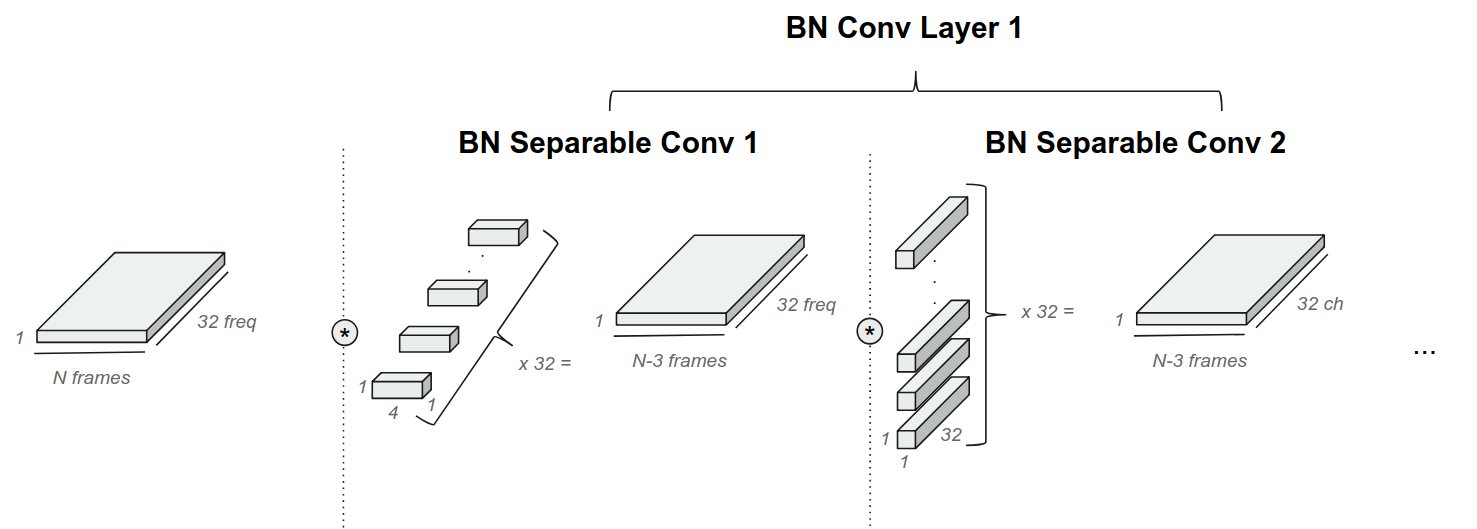
Fig. 1: The default configuration of a bottleneck layer running on the DSP; here we see a kernel size of 4 applied in a frequency separable way, followed by one frequency kernel per output channel. These two convolutions are considered as a single ’layer’.

2 Related Work

Fully end-to-end LVCSR are emerging as the state-of-the-art [2], equalling and even surpassing the performance of standard connectionist temporal classification [3] models. The core architecture for these end-to-end models, called Listen, Attend, and Spell [4], contains three major subgraphs - an encoder, an attention mechanism, and a decoder. Since their proposal in 2015, there has been a substantial amount of work done to optimize these models for on-device use [5, 6], including weight matrix factorization, pruning, and model distillation. Due to these improvements, it is now possible to run a state-of-the-art LVCSR model on a mobile device’s core processor (at a high power cost).

For the traditional hidden markov model (HMM)-based systems that predate LAS architectures, neural networks (NN) had been heavily used as part of a traditional ASR acoustic model. [7] show that convolutional bottleneck compression improves system performance in such setups. Typically, these compressed representations are concatenated with small time-window features to provide ’context’.

Additionally, small HMM-based keyword spotters have been successfully optimized across a DSP and main processor. [8] propose a model which introduces $5\text{\,}\mathrm{-}$ and $6\text{\,}\mathrm{b}\mathrm{i}\mathrm{t}$ weight quantization for a reduced memory footprint without a significant reduction in accuracy. Although these models have different architectures and applications, their use of convolutional bottleneck features and fixed-point network quantization inform our architecture.

[8], [1] introduce a split across a fixed-point DSP and a main processor motivated by power optimization. A quantized, two-stage, separable convolutional layer running on the DSP forms the basis of their music detector. We use the same layer structure in our DSP implementation.

The previously mentioned approaches do not attempt to compress audio features before caching, but there are other analyses of the trade-off between feature caching and power savings in the literature. In [9] and [10], empirical power consumption drops from $700\text{\,}\mathrm{m}\mathrm{W}$ to $25\text{\,}\mathrm{m}\mathrm{W}$ as data is cached $50\text{\,}\mathrm{x}$ longer for a pedometer application. Measurements of [1] indicate a full $25\text{\,}\%$-$50\text{\,}\%$ of the power cost at inference time is due to fixed wakeup and sleep overhead. Our goal is to significantly reduce this fixed power cost.

3 Feature Substitution

State-of-the-art results are reported in [2] with a very large, proprietary corpus. In this paper, we use the Librispeech 100 corpus to train our model [11]. [2] report a WER of $4.1\text{\,}\%$ with over 12,500 hours of training data; the same model trained on 100 hours of Librispeech data gives a WER of $21.8\text{\,}\%$, which we use as the baseline for all further evaluation.

The model from [2] is capable of running on a phone using 80-dimensional, $32\text{\,}\mathrm{b}\mathrm{i}\mathrm{t}$ floating point mel spectrum audio features sampled in $25\text{\,}\mathrm{m}\mathrm{s}$ windows every $10\text{\,}\mathrm{m}\mathrm{s}$. These features capture a maximum frequency of $7.8\text{\,}\mathrm{k}\mathrm{H}\mathrm{z}$ and are stacked with delta and double delta features, resulting in an 80 x 3 input vector at each timestep. We replace these features with quantized mel features (QM-features) that are compact, simple to calculate, and currently in use by other services running on the DSP.

QM-features are log-mel based with a $16\text{\,}\mathrm{b}\mathrm{i}\mathrm{t}$ fixed point representation. We use a default, narrow-band frequency representation that only captures up to $3.8\text{\,}\mathrm{H}\mathrm{z}$ over 32 bins. We test the effect of reducing the bandwidth by simply using fewer log-mel bins. Sampling rate and window size are constant across test input features and, for each case, we train an end-to-end model. The results of training a state-of-the-art LAS model with different input representations which can be calculated and cached on the DSP can be seen in Table 1.

Model Input	Input Dims	Feature Type	WER (%)	bandwidth (BW) (kbps)
$16\text{\,}\mathrm{k}\mathrm{H}\mathrm{z}$ $16\text{\,}\mathrm{b}\mathrm{i}\mathrm{t}$ raw PCM audio	–	–	–	256
Baseline LAS Model	80 x 3	Mel, +$\Delta$ +$\Delta\Delta$	21.79	768
Standard QM-features + Deltas	32 x 3	Mel, +$\Delta$ +$\Delta\Delta$	22.42	154
Standard QM-features	32 x 1	Mel	22.62	51.2
3/4 BW QM-features	24 x 1	Mel	22.80	38.4
1/2 BW QM-features	16 x 1	Mel	22.97	25.6
1/4 BW QM-features	8 x 1	Mel	24.52	12.8

Table 1: Comparison of model performance with smaller feature representations.

The results indicate that the baseline model, whose features have not previously been optimized, has a heavily redundant input representation, requiring three times the BW of the raw audio after delta stacking. We are able to significantly reduce the input BW (and, by extension, the amount of computation in the initial LAS layers) without severely affecting the model’s WER.

Delta- and double delta- feature stacking do not have a large effect relative to their $3\text{\,}\mathrm{x}$ increase in size; thus we will take the standard $32\text{\,}\mathrm{b}\mathrm{i}\mathrm{n}$ QM-features input as our starting point for further exploration. Though we see an incremental trade-off between BW and WER for smaller raw feature representations, we will use the full $32\text{\,}\mathrm{b}\mathrm{i}\mathrm{n}$ QM-features as an input to our compressived bottleneck layers in an attempt to preserve WER while reducing the BW even more drastically.

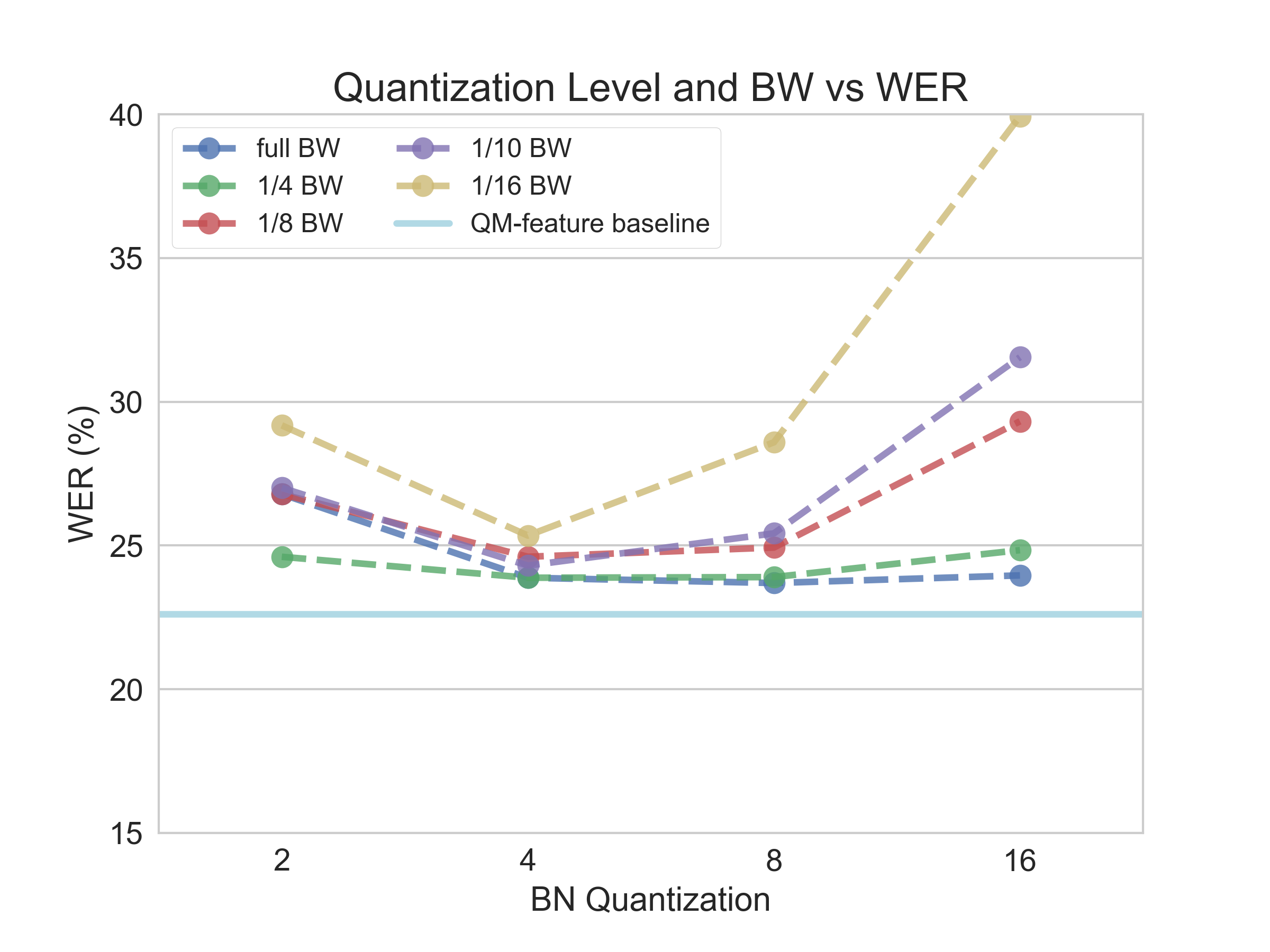
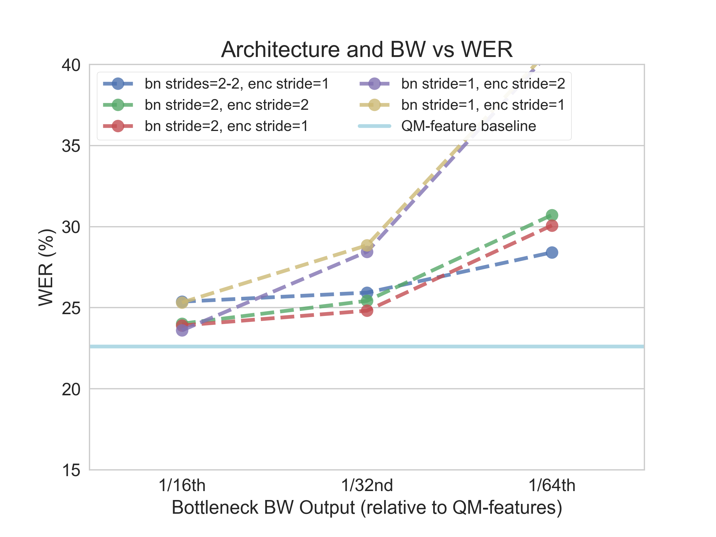
Fig. 2: The left plot uses a bottleneck feature extractor with a single hidden layer in which the output layer dimension and quantization level were modified to give a certain bandwidth output (relative to the standard $32\text{\,}\mathrm{d}$imensional $16\text{\,}\mathrm{b}\mathrm{i}\mathrm{t}$ QM-features). We see a trend towards 4-bit quantization, especially at high compression levels. The right plot shows the performance of various architectures (different bottleneck and encoder depths/strides and BNF dimension) at 4-bit quantization, plotted against bandwidth. As more drastic compression is demanded, shifting the stride to before the BNFs improves performance, which is similar to reducing the frame rate in more traditional models [12].

4 Bottleneck Feature Extraction

Our model uses the convolutional structure outlined by [1]. The structure of a single layer is shown in Figure 1. These simple, separable convolutional layers have been optimized for the DSP. Besides minimal computation, all layer weights and intermediate representations are quantized to $8\text{\,}\mathrm{b}\mathrm{i}\mathrm{t}\mathrm{s}$. $32\text{\,}\mathrm{b}\mathrm{i}\mathrm{t}$ biases, batch normalization [13], and a restricted linear unit (ReLU) activation function are included after the second, 1-D separable convolution.

To explore the space of bottleneck architectures, we parameterized this architecture along the following axes: output dimension size, output quantization level, convolutional stride (in time), kernel size, and the number of layers in the bottleneck network. The first three axes have the potential to reduce the BW of the resulting bottleneck, while the latter two axes are relevant to the size of the resulting model. Reducing the output dimension size is equivalent to reducing the size of the bottleneck layer and can result in a proportional reduction in BW. The output quantization level affects how many bits are saved for each of the values in the output, and will also result in a proportional reduction in BW. Increasing the stride could exponentially decrease the BW, for example, by doubling the stride we generate outputs only half as often.

These changes in input lead to a necessary modification of the initial two convolutional layers of the LAS encoder, which are designed with 3x3 time-frequency kernels and strides of 2. We replace these (by default) with a 3x1 time kernel along the flattened and modified frequency axis. We also vary the number of initial encoder layers and strides in our analysis.

5 Results

Model	$\#$ BNF Extractor Weights	$\Delta$ LAS Encoder Weights	Total Stride	BW (kbps)	WER (%)
16kHz 16-bit Raw PCM Audio	–	–	–	256	–
Baseline LAS Model	–	0 (0)	4	768	21.79
Standard QM-features	0 (0)	-3,072 (-98KB)	4	51.2	22.62
Best ~1/10 BW. BNF Model, $\nabla$	512 (4KB)	-8,064 (-258KB)	1	4.8	22.44
Best ~1/20 BW. BNF Model, $\nabla$	512 (4KB)	-8,064 (-258KB)	2	2.4	23.55
Best 1/32 BW. BNF Model, $\nabla$	384 (3KB)	-8,448 (-270KB)	2	1.6	24.81
Best 1/16 BW. BNF Model	640 (5KB)	-7,680 (-246KB)	4	3.2	24.02
1/32 BW. BNF Model	384 (3KB)	-8,448 (-270KB)	4	1.6	25.42
Best 1/64 BW. BNF Model	1536 (123KB)	-8,448 (-270KB)	4	0.8	28.41

Table 2: Selection of best performing models for different bandwidths.

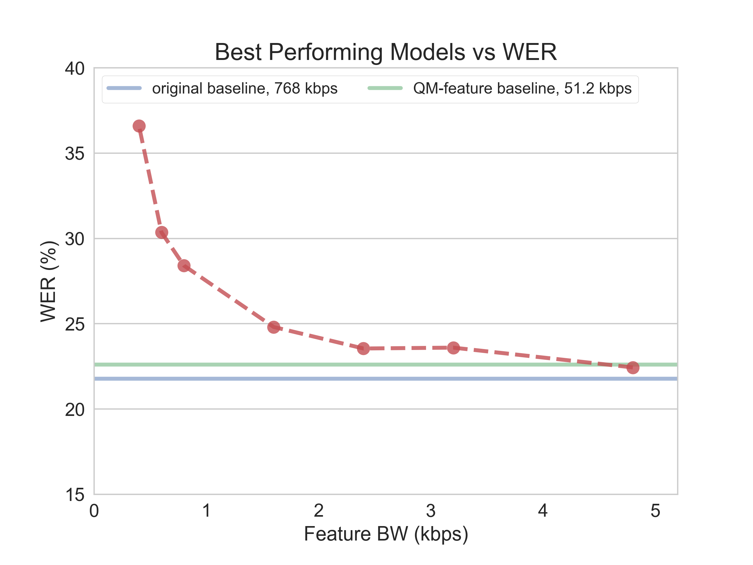
Fig. 3: Best performing model vs bandwidth. We see a good trade-off around $2\text{\,}\mathrm{k}\mathrm{b}\mathrm{p}\mathrm{s}$.

Initial results are based on freezing the bottleneck (BN) extractor and encoder layer parameters and varying one parameter at time. This analysis revealed a statistically insignificant effect of BN kernel size (across a range from 1 to 10) based on McNemar statistical tests [14]. Activation function comparisons favored ReLU in a default configuration, but at high levels of quantization/compression showed no difference between identity and ReLU activation functions.

There was a clear performance loss when increasing BN stride without a simultaneous decrease in encoder stride. We hypothesize that the model has already been optimally compressed in the time dimension (the original model has a time step of $10\text{\,}\mathrm{m}\mathrm{s}$ fed through two strides of two, resulting in an encoded frame every $40\text{\,}\mathrm{m}\mathrm{s}$). No dependence on encoder depth was noticeable.

In Figure 2, we see the results of varying the BNF output dimension and quantization level at different rates of compression relative to the $32\text{\,}\mathrm{d}$imensional $16\text{\,}\mathrm{b}\mathrm{i}\mathrm{t}$ QM-features. A quantization of $4\text{\,}\mathrm{b}\mathrm{i}\mathrm{t}\mathrm{s}$ and 8-12 output dimensions perform the best across compression levels.

The best performing models have been collected in Table 2. Each of these models has a single hidden layer in the BNF extractor with the exception of the 1/64 BW model, and a stride of two in the bottleneck layer with the exception of the 1/10 BW model. All of the models have an output quantization depth of $4\text{\,}\mathrm{b}\mathrm{i}\mathrm{t}\mathrm{s}$, a kernel of 4, and output dimensionality between 8 and 16 channels. They use single convolutional layer with a stride of 1 in the encoder (excepting the 1/16 and 1/32 constant time compression models, which have a stride of 2).

Our optimized $4.8\text{\,}\mathrm{k}\mathrm{b}\mathrm{p}\mathrm{s}$ model with a single BNF layer actually outperforms the standard QM-features model (running at $51.2\text{\,}\mathrm{k}\mathrm{b}\mathrm{p}\mathrm{s}$). Compared with the original unoptimized model, this is a $160\text{\,}\mathrm{x}$ reduction in feature bandwidth for a $0.6\text{\,}\%$ increase in WER. We are able to continue to compress our BNFs more and more heavily for slight increases in WER. Our presented system is able to reduce the footprint of standard fixed point DSP spectral features by a factor of 64 for a $5.8\text{\,}\%$ relative increase in WER; compared with the original floating point model, this represents a $960\text{\,}\mathrm{x}$ feature compression for a $6.6\text{\,}\%$ increase in WER. The best performing models at ~1/84 ($0.6\text{\,}\mathrm{k}\mathrm{b}\mathrm{p}\mathrm{s}$) and 1/128 ($0.4\text{\,}\mathrm{k}\mathrm{b}\mathrm{p}\mathrm{s}$) converge to WER values of $30.36\text{\,}\%$ and $36.59\text{\,}\%$ respectively, which represents the breakdown in performance (Figure 3).

6 Conclusion

Our analysis revealed that time compression was initially the limiting factor in our model, and a $40\text{\,}\mathrm{m}\mathrm{s}$ compressed step size seems to be the limit for high accuracy models. We found that kernel dimensionality and activation function had little effect on our results, and $4\text{\,}\mathrm{b}\mathrm{i}\mathrm{t}\mathrm{s}$ quantization with 8-12 dimensional BNFs per timestep performed optimally.

Given these findings, we were able to design several models that effectively compress audio features on the DSP and allow them to be cached in severely reduced memory footprints. We designed a model that successfully compresses the original DSP QM-features to 1/10 the size without any loss in accuracy. As we compress the features further, we find an inflection point in WER around $1\text{\,}\mathrm{k}\mathrm{b}\mathrm{p}\mathrm{s}$.

While the models we have designed can increase the interval between main processor wake-ups by $10\text{\,}\mathrm{x}$-$64\text{\,}\mathrm{x}$, empirical data is necessary to understand the full effect on battery consumption. Some of our models require slightly more computation in the attention/decoder (because of decreased time compression), which alone may have an adverse effect on battery life. Further tuning should be done once these are tested in-situ.

These BNFs may be useful for other compressed speech models, and the end-to-end training paradigm, while time-consuming, provides an optimal means for on-DSP compression. We hope this architecture is adopted in portable applications as a standard technique for speech compression.

Acknowledgments

The authors would like to acknowledge Ron Weiss and the Google Brain and Speech teams for their LAS implementation, Félix de Chaumont Quitry and Dick Lyon for their feedback and support, and the Google AI Zürich team for their help throughout the project.

References

- [1] Beat Gfeller et al. “Now Playing: Continuous low-power music recognition” In arXiv preprint arXiv:1711.10958, 2017
- [2] Chung-Cheng Chiu et al. “State-of-the-art speech recognition with sequence-to-sequence models” In 2018 IEEE International Conference on Acoustics, Speech and Signal Processing (ICASSP), 2018, pp. 4774–4778 IEEE
- [3] Alex Graves “Connectionist Temporal Classification” In Supervised Sequence Labelling with Recurrent Neural Networks Springer, 2012, pp. 61–93
- [4] William Chan, Navdeep Jaitly, Quoc Le and Oriol Vinyals “Listen, attend and spell: A neural network for large vocabulary conversational speech recognition” In Acoustics, Speech and Signal Processing (ICASSP), 2016 IEEE International Conference on, 2016, pp. 4960–4964 IEEE
- [5] Rohit Prabhavalkar, Ouais Alsharif, Antoine Bruguier and Ian McGraw “On the compression of recurrent neural networks with an application to LVCSR acoustic modeling for embedded speech recognition” In arXiv preprint arXiv:1603.08042, 2016
- [6] Ruoming Pang et al. “Compression of End-to-End Models” In Proc. Interspeech 2018, 2018, pp. 27–31
- [7] Karel Veselỳ, Martin Karafiát and František Grézl “Convolutive bottleneck network features for LVCSR” In Automatic Speech Recognition and Understanding (ASRU), 2011 IEEE Workshop on, 2011, pp. 42–47 IEEE
- [8] Mohit Shah et al. “A fixed-point neural network architecture for speech applications on resource constrained hardware” In Journal of Signal Processing Systems 90.5 Springer, 2018, pp. 727–741
- [9] Bodhi Priyantha, Dimitrios Lymberopoulos and Jie Liu “Littlerock: Enabling energy-efficient continuous sensing on mobile phones” In IEEE Pervasive Computing 10.2 IEEE, 2011, pp. 12–15
- [10] N Priyantha, Dimitrios Lymberopoulos and Jie Liu “Eers: Energy efficient responsive sleeping on mobile phones” In Proceedings of PhoneSense 2010, 2010, pp. 1–5
- [11] Vassil Panayotov, Guoguo Chen, Daniel Povey and Sanjeev Khudanpur “Librispeech: an ASR corpus based on public domain audio books” In Acoustics, Speech and Signal Processing (ICASSP), 2015 IEEE International Conference on, 2015, pp. 5206–5210 IEEE
- [12] Golan Pundak and Tara Sainath “Lower Frame Rate Neural Network Acoustic Models” In Interspeech, 2016
- [13] Sergey Ioffe and Christian Szegedy “Batch normalization: Accelerating deep network training by reducing internal covariate shift” In arXiv preprint arXiv:1502.03167, 2015
- [14] Quinn McNemar “Note on the sampling error of the difference between correlated proportions or percentages” In Psychometrika 12.2 Springer, 1947, pp. 153–157