PROPERTIES OF TURBULENCE IN THE RECONNECTION EXHAUST: NUMERICAL SIMULATIONS COMPARED WITH OBSERVATIONS

Abstract

The properties of the turbulence which develops in the outflows of magnetic reconnection have been investigated using self-consistent plasma simulations, in three dimensions. As commonly observed in space plasmas, magnetic reconnection is characterized by the presence of turbulence. Here we provide a direct comparison of our simulations with reported observations of reconnection events in the magnetotail investigating the properties of the electromagnetic field and the energy conversion mechanisms. In particular, simulations show the development of a turbulent cascade consistent with spacecraft observations, statistics of the the dissipation mechanisms in the turbulent outflows similar to the one observed in reconnection jets in the magnetotail, and that the properties of turbulence vary as a function of the distance from the reconnecting X-line.

1 Introduction

Turbulence and magnetic reconnection are two fundamental phenomena in space plasmas. The former is responsible for the cascade of magnetic and ordered kinetic energy from large scale, where the energy is injected, to small scales, where the energy can be transformed to particle heating and acceleration. The latter consists in the reconfiguration of magnetic field topology with the effect of decreasing magnetic energy in favor of particle heating or acceleration. These two phenomena are not separate in nature, but on the contrary they often go “hand-in-hand” (Matthaeus & Velli, 2011). The effects of turbulence on magnetic reconnection have been widely studied in magnetohydrodynamics (MHD) (Matthaeus & Lamkin, 1986; Lazarian & Vishniac, 1999; Loureiro et al., 2007, 2009; Kowal et al., 2012), while remaining not well-understood in the context of collisionless plasmas. It has also been shown that the generation of strong small-scale current sheets in the turbulent cascade provides the conditions for the onset of reconnection, making the latter a fundamental ingredient of the former (Servidio et al., 2009, 2011). On the other hand, the self-generation of turbulence in magnetic reconnection has been studied as well theoretically in two-dimensional (2D) numerical simulation of MHD (Matthaeus & Lamkin, 1986; Malara et al., 1991, 1992; Lapenta, 2008; Bhattacharjee et al., 2009).

In the recent years, thanks to the steady increase of the available computational resources, the full self-consistent description of three-dimensional (3D) reconnection has become a reality. It has been shown that in 3D new phenomena arise that change the picture of how and where the magnetic energy is converted to plasma energy (Daughton et al., 2011; Lapenta et al., 2015). Many of these discoveries concern the physics of the outflows of reconnection: Vapirev et al. (2013) showed that an interchange instability develops at the interface between the plasma ejected from the first reconnection site and the ambient plasma; Lapenta et al. (2015) that in the reconnection outflows a large number of secondary reconnection sites develops; and Leonardis et al. (2013) that intermittent turbulence develops in the outflows.

Observations reveal the presence of a large number of reconnection events, from large to small scales (Retinò et al., 2007; Greco et al., 2016). Analogously, it is commonly observed that large scale exhausts are far from being in a laminar and regular regime, showing instead the clear manifestation of turbulence (Osman et al., 2015). More specifically, spacecraft observations of reconnection have also revealed the presence of turbulence within the ion diffusion region (Eastwood et al., 2009). In the inertial subrange, electric and magnetic fluctuations both followed a classical $k^{-5/3}$ power law; at higher frequencies, the spectral indices were near $-1$ and $-8/3$, respectively.

In this paper, motivated by spacecraft observations, such as the studies by  Eastwood et al. (2009) and Osman et al. (2015), we study the properties of turbulence in the outflows of reconnection by means of a 3D kinetic numerical simulation. We recover many features of turbulence that develop in the reconnection outflows as observed in the Earth magnetotail. We show that a turbulent energy spectrum develops at kinetic scale as a consequence of reconnection. The slope of the electric and magnetic energy spectra at ion scales are found to be consistent with observation, along with the scale at which the two spectra depart one from the other. We better characterize where and how the energy exchange between fields and particles happens in a reconnection event. Our results show that dissipation takes place manly in the outflows and it is intermittent. Moreover, we show how the properties of the turbulence varies moving away from the X-point in the outflow direction. Our results are relevant to the physics of the magnetotail and could be useful to better understand the ongoing Magnetospheric MultiScale (MMS) Mission observation of that region.

2 Numerical simulation and analysis

In our simulation, we consider a plasma made of protons and electrons. The initial configuration is the classical Harris-equilibrium:

$${\bf B}=B_{0x}\tanh(y/\delta){\bf e_{x}}+B_{0z}{\bf e_{z}}$$

$$n=n_{0b}+\frac{n_{0}}{\cosh^{2}(y/\delta)}.$$

The coordinates are chosen as: $x$ along the sheared component of the magnetic field (Earth-Sun direction in the Earth magnetotail), $y$ in the direction of the gradients (north-south in the magnetotail), and $z$ along the current and the guide field (dawn-dusk in the magnetotail). For both species, the particle distribution function is Maxwellian with spatially homogeneous temperature. A uniform background $n_{0b}$ is added in the form of a non-drifting Maxwellian at the same temperature of the main Harris plasma. We solve the Vlasov-Maxwell equations for the two species using the semi-implicit Particle In Cell code iPIC3D (Brackbill & Forslund, 1982; Markidis et al., 2010; Lapenta, 2012). We consider a 3D box of shape $[40,15,10]\,d_{p}$, where $d_{p}$ is the proton inertial length, which is resolved by a Cartesian grid of $[720,270,228]$ cells, each one initially populated with $125$ particles. We use a realistic mass ratio, $m_{p}/m_{e}=1836$, which fixes the spatial resolution to $\Delta x=d_{p}/18\sim 2d_{e}$, where $d_{e}$ is the electron inertial length. The proton and electron thermal speeds are $0.0063c$ and $0.12c$ respectively at the initial time, where $c$ is the speed of light, resulting in a temperature ratio of $T_{p}/T_{e}=5$. The thickness of the initial current sheet is set to $\delta=0.5d_{p}$, the density of the background such that $n_{0b}/n_{0}=0.1$, and the case of small guide field is considered: $B_{0z}/B_{0x}=0.1$. We impose open boundary conditions in the $x$ and $y$ direction, and periodicity along $z$. The magnetic reconnection process is initialized with a perturbation of the $z$ component of the vector potential localized in the center of the domain (Vapirev et al., 2013). The plasma ejected from the first reconnection sites encounters the ambient plasma and piles up forming the reconnection front. This front is unstable producing magnetic fluctuations and initiating the turbulent cascade. It moves towards the boundaries and eventually exits the simulation box. We stop the simulation when the reconnection front has already started moving and is far enough from both the boundaries to study the turbulence that develops in front of it. This time corresponds to $t\approx 23.3\Omega_{cp}$, where $\Omega_{cp}$ is the proton cyclotron frequency computed using the asymptotic magnetic field, which is the time at which we performed the bulk of our analysis.

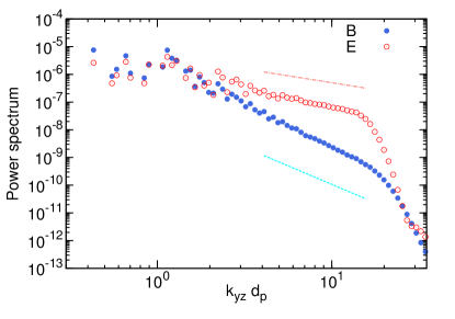
Figure 1: Power spectra of magnetic (blue bullets) and electric (open red circles) fields as a function of the perpendicular $k$-vector (with respect to the reconnecting field direction). Spectra have been reduced along $k_{x}$. Dashed (red) line and dot-dashed (blue) lines indicate the behavior of the observations for the magnetic ($\propto k^{-8/3}$) and electric spectra ($\propto k^{-1}$), respectively.

2.1 Electric and magnetic spectra

In order to establish a first connection between plasma simulations of turbulent reconnection and the observations, we computed the power spectral densities of the fluctuations. Because of the inhomogeneous background, it is important to first establish the anisotropy level and, in general, the 3D properties of turbulence. As we are interested in the fluctuations produced by magnetic reconnection, we define the magnetic fluctuations as

$${\bf b}({\bf x})={\bf B}({\bf x})-\langle B_{x}({\bf x})\rangle_{x,z}{\bf e}_{x}-\langle{\bf B}({\bf x})\rangle_{x,y,z}$$

where $\langle\bullet\rangle$ represents spatial averaging in the (2 or 3) directions indicated by the suffix. The above definition subtracts both mean fields and the large-scale shear: the second term in the right-hand side represents the signature of the background Harris sheet that is still present at the time we are analyzing, while the last term is the (small) guide field. The reduced auto-correlation function, computed in each direction, averaging over the entire volume, is defined as $C(r_{j})=\langle{\bf b}({\bf x}+r_{j}\hat{{\bf r}}_{j})\cdot{\bf b}({\bf x})\rangle_{x,y,z}/b^{2}$. Here $j=x,y,z$, ${\hat{\bf r}}_{j}$ are the unit vectors in the three directions, and $b^{2}$ the average magnetic energy of the fluctuations, i. e. $b^{2}=C(0)$.

In an infinite size system, for regular statistics, the autocorrelation function tends to zero for large values of the displacements, indicating convergence of the moments. We computed $C(r_{j})$ at the peak of the nonlinear activity, measuring the correlation length of the fluctuations $\lambda_{C_{j}}$ as the displacement at which the correlation function is reduced by a factor $1/e$. Using this $e$-folding procedure, we measured: $\lambda_{C_{x}}=4.4d_{p}$, $\lambda_{C_{y}}=2.8d_{p}$, and $\lambda_{C_{z}}=1.7d_{p}$. This difference between correlation lengths indicates spectral (or correlation) anisotropy among the three main directions. The large scale (energy containing) vortexes are more elongated in the $x$ direction (along the reconnecting field). There is a secondary anisotropy due to the presence of the shear along $y$, which suggest that the coherent structures have the shortest extension along the periodic direction $z$. This observation is therefore in agreement with the anisotropic geometry of the problem.

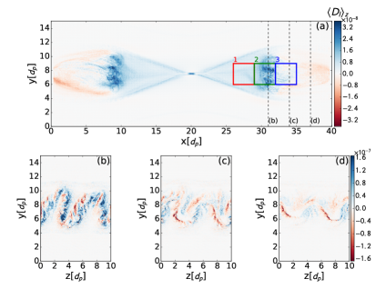
Figure 2: Energy exchange $D_{l}={\bf J}\cdot{\bf E}$ in the $xy$ plane averaged in the $z$ direction (a), and in the $yz$ plane at $x=31\,d_{p}$ (b), $x=34\,d_{p}$ (c), $x=37\,d_{p}$ (d). The x-line is located at $x=20\,d_{p}$. The three boxes in panel (a) are the ones used for the statical analysis presented in Section 2.2.

In order to compute the power spectra, we used Hanning-windowing in the $x$ and $y$ directions, isolating the central exhausts. The window size and sharpness has been varied, verifying that the chosen parameters do not alter the spectrum significantly. Three dimensional energy spectra of the magnetic field confirm what was found about the correlation lengths. It is worth noting, however, that the main anisotropy direction is along $x$, and that the anisotropy in the $yz$ plane is smaller, and is negligible at scales $r\ll\lambda_{C_{z}}$. This effect of isotropization is typical of small-scale turbulence. In our case, isotropy is recovered in the $(k_{y},k_{z})$ plane for $k_{yz}d_{p}>1.5$, with $k_{yz}=\sqrt{k_{y}^{2}+k_{z}^{2}}$. Therefore it is reasonable to compute the total energy spectrum by integrating over $k_{x}$ and computing concentric isotropic shells in the $(k_{y},k_{z})$ plane. The results for the electric and magnetic energy are shown in Figure 1. In agreement with space plasma observations (Bale et al., 2005; Eastwood et al., 2009), the two spectra exhibit a different power law decay at proton scales, with the electric spectrum proceeding at sub-proton scales with spectral index $\sim-1$, while the magnetic behaves more like $\sim k^{-8/3}$. The characteristic spatial scale at which the two spectra depart is $kd_{p}\sim 1$, in accordance with observations. In order to compare the two spectral indexes, the electric field power spectrum has been rescaled by a factor $5\times 10^{3}$.  Eastwood et al. (2009) found a factor of $\sim 9\times 10^{4}$, an order of magnitude larger. However, in our simulation the Alfvén speed and the ion thermal speed are $\sim 1.5$ and $\sim 3.0$ times bigger than their typical values in observation. From a dimensional analysis of Faraday’s law we get that $E/B\approx v$, where $E$, $B$ and $v$ are characteristic quantities. Hence, it is expected that the electric activity will increase if the typical plasma velocities increase.

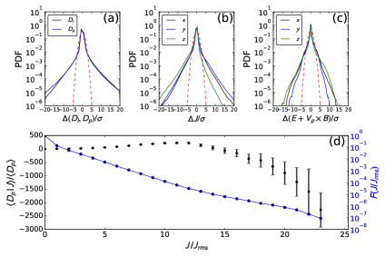
Figure 3: PDFs of $D_{l}$ and $D_{p}$ (a), $\bf{J}$ (b), and $\bf{E}_{p}$ (c). Red dashed lines represent the normalized Gaussian curve. Mean $D_{p}$ conditioned on local current density thresholds and (right axis) fraction $F$ of the full box data used to compute the averages (d).

2.2 Energy exchange between fields and particles

The energy exchange between fields and particles is governed by the term ${\bf J}\cdot{\bf E}$, where ${\bf J}$ is the total current, sum of protons and electrons contributions, and ${\bf E}$ is the electric field. When $D_{l}={\bf J}\cdot{\bf E}$ is positive the energy is flowing from the fields to the particles, when it is negative energy is passing from particles to fields. It is sometimes referred to as the “dissipative” term, even though the energy transfer from magnetic field to particles is not always an irreversible process, and so it does not strictly imply dissipation. Despite this fact, for the purpose of our paper we will keep this definition, also used elsewhere (Zenitani et al., 2011; Olshevsky et al., 2015, 2016), and from now on we will use $D_{l}$ as a proxy for dissipation or more properly energy release from the electromagnetic field (in the laboratory frame). A 2D plot of $D_{l}$ integrated in the $z$ direction is shown in Figure 2. As shown in other works, in collisionless magnetic reconnection $D_{l}$ is not concentrated only around the first reconnection site (Lapenta et al., 2014, 2015). In fact, it takes nonzero values in a wider region contained in the outflows (panel (a)). Moreover, $D_{l}$ is strongly inhomogeneous inside the outflows. In order to characterize this inhomogeneity we plotted $D_{l}$ in the plane facing the outflows, $yz$, at three different positions along $x$: $31d_{p}$, $34d_{p}$, and $37d_{p}$. The largest values of $D_{l}$ are found in the region where the plasma ejected by reconnection encounters the ambient plasma and is decelerated, near $x=31d_{p}$ in the right outflow. This region is characterized by an interface instability, which was studied in Vapirev et al. (2013). $D_{l}$ is stronger in that position and decreases moving outwards from the first reconnection site in the outflow direction. Note that $D_{l}$ has in general both positive and negative values, but in the considered region its average is always positive, indicating a net flow of energy from fields to particles.

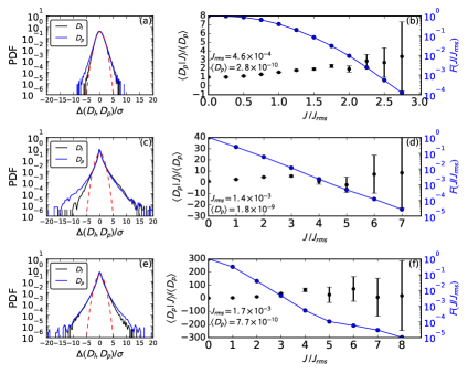
Figure 4: PDFs of $D_{l}$ and $D_{p}$ in $BOX_{1}$ (a), $BOX_{2}$ (c), and $BOX_{3}$ (e). Conditioned average of $D_{p}$ and filling factors $F$ in $BOX_{1}$ (b), $BOX_{2}$ (d), and $BOX_{3}$ (f).

In order to give a better description of how energy is converted and to compare our results with observations, we performed a statistical analysis similar to what presented by Osman et al. (2015), where a dissipation analysis was performed on observational data in a magnetic reconnection outflow in the magnetotail. It is worth noticing that in Osman et al. (2015) the statistics were made from temporal data collected by the satellites crossing the reconnection outflow, while in our case the whole simulation box is used as a single sample.

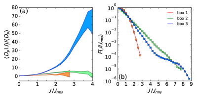
Figure 5: Conditioned average of $D_{p}$ (a) and filling factor (b) in BOX 1 (red), BOX 2 (green), and BOX 3 (blue).

In panel (a) of Figure 3 the Probability Density Functions (PDFs) of $D_{l}$ and $D_{p}$ are plotted. $D_{p}$ represents the dissipation proxy in the proton reference frame and is given by $D_{p}={\bf J}\cdot{\bf E}_{p}$, where ${\bf E}_{p}=\left({\bf E}+{\bf V}_{p}\times{\bf B}\right)$ is the electric field in the proton reference frame, ${\bf V}_{p}$ representing the proton bulk velocity. The two PDFs are compared with the normalized Gaussian distribution (plotted in dashed-red line). They strongly depart from Gaussian distributions, presenting instead high tails up to several standard deviations $\sigma$, which can be interpreted as a signature of intermittency. In panel (b) and (c), we present separately the PDFs of the two terms which compose $D_{p}$. In agreement with what was found in the space measurement, the PDFs of ${\bf J}$ and ${\bf E}_{p}$ are both non-Gaussian. In panel (d), the average $D_{p}$ conditioned to a threshold current density is shown. The plot is constructed as follows: a threshold in the current density magnitude is considered and the average of $D_{p}$ is computed using all those points in the domain where the value of the current is bigger than the fixed threshold. This average is then normalized to the average of $D_{p}$ on all points, which gives by definition $\langle D_{p}|J=0\rangle/\langle D_{p}\rangle=1$. The black points in the plots represent the result of such computation for different values of the threshold. The blue curve represents the filling factors, i.e. the fraction of points used for computing the average with respect to the total number of points in the sample. The average of $D_{p}$ strongly increases when higher threshold are considered up to $J/J_{rms}=10$. Beyond this threshold, the average starts decreasing and changes sign to reach large negative values for the strongest current density. Our results confirms that the exchange of energy is local, with larger values of $|D_{p}|$ localized in very small volume filling structures. We show as well that even if the average of $D_{p}$ is positive, points where the value of the current is very strong can be site of negative $D_{p}$. This is not a universal behavior, but indeed depends on the particular time considered in the simulation: we performed the same analysis at a different time step (not shown) finding positive values of $D_{p}$ for big current values. However, at all times the energy exchange is consistently concentrated in small regions, where the values of $D_{p}$ is much larger than its global average.

The above statistical analysis was performed considering the whole simulation box, providing information about the average properties of the dissipation proxy in the reconnection events. In order to obtain a more detailed description, and to identify in which place the energy exchange actually occurs we perform the previous statistical analysis in three different regions of the simulation, by selecting three boxes located in the left reconnection outflows at three different distances from the X-point. The boxes are identified by $6<y/d_{p}<9$ (reconnection zone), $0<z/d_{p}<10$ (full domain in $z$), and with ${\mbox{BOX}}_{1}=\left\{26<x/d_{p}<29\right\}$, ${\mbox{BOX}}_{2}=\left\{29<x/d_{p}<32\right\}$, ${\mbox{BOX}}_{3}=\left\{32<x/d_{p}<35\right\}$ (see Figure 2). Moving further in the direction of the outflows the PDFs become non-Gaussian. This transition happens between $BOX_{1}$ and $BOX_{2}$ (Figure 4, panels a-c). Moreover, passing from $BOX_{2}$ to $BOX_{3}$ the PDFs of $D_{p}$ and $D_{l}$ become more similar, suggesting that proton inertia become less important in the exhaust of reconnection. The evolution of the conditioned average is interesting as well (Figure 4, panels b-d-f). Moving from $BOX_{1}$ to $BOX_{3}$ the conditioned average of $D_{p}$ increases for bigger values of the current density threshold. This is more evident in the direct comparison shown in Figure 5, where the normalized conditioned average grows from $BOX_{1}$ to $BOX_{3}$ (panel a). Similarly, the structures filling factor shows higher tails passing from $BOX_{1}$ to $BOX_{2}$ and $BOX_{3}$.

3 Conclusions

We have used a 3D kinetic numerical simulation to study the properties of the turbulence that develops in the outflow of magnetic reconnection using parameters typical of the Earth magnetotail. Simulations have shown that such turbulence is anisotropic, with large scales dominated by fluctuations whose wavevector is directed in the direction of the reconnecting magnetic field. Magnetic and electric turbulent energy spectra follows two different power laws at scales smaller than the proton inertial length, with slopes which are in agreement with observations. Like the turbulent activity, the energy exchange between fields and particles is concentrated in the outflows, where the strongest values of dissipation are found at the interface between the plasma ejected by reconnection and the ambient plasma. Statistical analysis of the dissipation proxy confirms that the energy exchange between fields and particles occurs in small volume filling structure where the value of the current is much stronger than its root mean square. The current sheets produced by the turbulent activity compared to their root mean square values are stronger in numerical simulation compared to observations. This difference could be due to the curlometer technique used to estimate current density from magnetic field measurements. Moreover, we showed that in those places where the value of the current densities are very high and which are not resolved by observations, the energy can also be transferred from particles to field. Finally, we showed that the properties of the turbulence produced in the outflows varies in space becoming more intermittent moving far from the X-point. We believe that these results could be used to better explain the upcoming MMS Mission observations of the magnetotail.

References

- Bale et al. (2005) Bale, S., Kellogg, P., Mozer, F., Horbury, T., & Reme, H. 2005, Physical Review Letters, 94, 215002
- Bhattacharjee et al. (2009) Bhattacharjee, A., Huang, Y.-M., Yang, H., & Rogers, B. 2009, Physics of Plasmas (1994-present), 16, 112102
- Brackbill & Forslund (1982) Brackbill, J., & Forslund, D. 1982, Journal of Computational Physics, 46, 271
- Daughton et al. (2011) Daughton, W., Roytershteyn, V., Karimabadi, H., et al. 2011, Nature Physics, 7, 539
- Eastwood et al. (2009) Eastwood, J., Phan, T., Bale, S., & Tjulin, A. 2009, Physical review letters, 102, 035001
- Greco et al. (2016) Greco, A., Perri, S., Servidio, S., Yordanova, E., & Veltri, P. 2016, The Astrophysical Journal Letters, 823, L39
- Kowal et al. (2012) Kowal, G., Lazarian, A., Vishniac, E. T., & Otmianowska-Mazur, K. 2012, Nonlinear Processes in Geophysics, 19, 297
- Lapenta (2008) Lapenta, G. 2008, Physical review letters, 100, 235001
- Lapenta (2012) —. 2012, Journal of Computational Physics, 231, 795
- Lapenta et al. (2014) Lapenta, G., Goldman, M., Newman, D., Markidis, S., & Divin, A. 2014, Physics of Plasmas (1994-present), 21, 055702
- Lapenta et al. (2015) Lapenta, G., Markidis, S., Goldman, M. V., & Newman, D. L. 2015, Nature Physics, 11, 690
- Lazarian & Vishniac (1999) Lazarian, A., & Vishniac, E. T. 1999, The Astrophysical Journal, 517, 700
- Leonardis et al. (2013) Leonardis, E., Chapman, S. C., Daughton, W., Roytershteyn, V., & Karimabadi, H. 2013, Physical review letters, 110, 205002
- Loureiro et al. (2007) Loureiro, N., Schekochihin, A., & Cowley, S. 2007, Physics of Plasmas, 14, 100703
- Loureiro et al. (2009) Loureiro, N., Uzdensky, D., Schekochihin, A., Cowley, S., & Yousef, T. 2009, Monthly Notices of the Royal Astronomical Society: Letters, 399, L146
- Malara et al. (1991) Malara, F., Veltri, P., & Carbone, V. 1991, Physics of Fluids B: Plasma Physics (1989-1993), 3, 1801
- Malara et al. (1992) —. 1992, Physics of Fluids B: Plasma Physics (1989-1993), 4, 3070
- Markidis et al. (2010) Markidis, S., Lapenta, G., et al. 2010, Mathematics and Computers in Simulation, 80, 1509
- Matthaeus & Lamkin (1986) Matthaeus, W., & Lamkin, S. L. 1986, Physics of Fluids (1958-1988), 29, 2513
- Matthaeus & Velli (2011) Matthaeus, W., & Velli, M. 2011, Space science reviews, 160, 145
- Olshevsky et al. (2016) Olshevsky, V., Deca, J., Divin, A., et al. 2016, The Astrophysical Journal, 819, 52
- Olshevsky et al. (2015) Olshevsky, V., Lapenta, G., Markidis, S., & Divin, A. 2015, Journal of Plasma Physics, 81, 325810105
- Osman et al. (2015) Osman, K., Kiyani, K., Matthaeus, W., et al. 2015, The Astrophysical Journal Letters, 815, L24
- Retinò et al. (2007) Retinò, A., Sundkvist, D., Vaivads, A., et al. 2007, Nature Physics, 3, 236
- Servidio et al. (2009) Servidio, S., Matthaeus, W., Shay, M., Cassak, P., & Dmitruk, P. 2009, Physical review letters, 102, 115003
- Servidio et al. (2011) Servidio, S., Dmitruk, P., Greco, A., et al. 2011, Nonlinear Processes in Geophysics, 18, 675
- Vapirev et al. (2013) Vapirev, A., Lapenta, G., Divin, A., et al. 2013, Journal of Geophysical Research: Space Physics, 118, 1435
- Zenitani et al. (2011) Zenitani, S., Hesse, M., Klimas, A., & Kuznetsova, M. 2011, Physical review letters, 106, 195003