PDE-constrained optimal control problems with uncertain parameters using SAGA

Abstract

We consider an optimal control problem (OCP) for a partial differential equation (PDE) with random coefficients. The optimal control function is a deterministic, distributed forcing term that minimizes an expected quadratic regularized loss functional. For the numerical approximation of this PDE-constrained OCP, we replace the expectation in the objective functional by a suitable quadrature formula and, eventually, discretize the PDE by a Galerkin method. To practically solve such approximate OCP, we propose an importance sampling version the SAGA algorithm [4], a type of Stochastic Gradient algorithm with a fixed-length memory term, which computes at each iteration the gradient of the loss functional in only one quadrature point, randomly chosen from a possibly non-uniform distribution. We provide a full error and complexity analysis of the proposed numerical scheme. In particular we compare the complexity of the generalized SAGA algorithm with importance sampling, with that of the Stochastic Gradient (SG) and the Conjugate Gradient (CG) algorithms, applied to the same discretized OCP. We show that SAGA converges exponentially in the number of iterations as for a CG algorithm and has a similar asymptotic computational complexity, in terms of computational cost versus accuracy. Moreover, it features good pre-asymptotic properties, as shown by our numerical experiments, which makes it appealing in a limited budget context.

35Q93, 49M99, 65C05, 65N12, 65N30

1 Introduction

In this paper we consider a risk averse optimal control problem (OCP) for a linear coercive PDE with random parameters of the form

(1) $$A_{\omega}y_{\omega}(u)=g_{\omega}+B_{\omega}u$$

where $\omega\in\Gamma$ denotes a random elementary event, $g_{\omega}$ is a random forcing term, $A_{\omega}$ is a random coercive differential operator, $u$ is the deterministic control function, whose action on the system is represented by the, possibly random, operator $B_{\omega}$, and $y_{\omega}(u)$ denotes the solution of the PDE corresponding to the control $u$ and random event $\omega$. The optimal control is the one that minimizes an expected tracking type quadratic functional

(2) $$u^{*}\in\operatorname*{arg\,min}_{u\in U}J(u):=\mathbb{E}_{\omega}[f(u,\omega)],\quad\text{with }f(u,\omega)=\frac{1}{2}\|H_{\omega}y_{\omega}(u)-z_{d}\|_{H}^{2}+\frac{\beta}{2}\|u\|^{2}_{U}.$$

Here, $H_{\omega}$ is an observation operator and $z_{d}$ the (deterministic) target observed state. The objective functional $J(u)$ includes a possible penalization term for well posedness. In the setting considered in this work, the function $u\mapsto f(u,\omega)$ is strongly convex for any $\omega\in\Gamma$ with Lipschitz continuous gradient (Gateaux derivative). We present in Section 3 of this work a specific example of a controlled diffusion equation with random diffusivity coefficient, which fits the general setting above.

The PDE-constrained OCP (1)-(2) is infinite-dimensional and, as such, has to be suitably discretized to be solved numerically. In this work, we focus on an approximation of the expectation operator by a suitable (deterministic or randomized) quadrature formula $\mathbb{E}[X]\approx\sum_{j=1}^{n}\zeta_{j}X(\eta_{j})$, with $X:\Gamma\to\mathbb{R}$ and integrable random variable, $\{\eta_{j}\}_{j}$ the quadrature knots and $\{\zeta_{j}\}_{j}$ the quadrature weights such that $\sum_{j=1}^{n}\zeta_{j}=1$. For example, one could use a Monte Carlo quadrature where $\eta_{j}$ are drawn independently from the underlying probability measure and the quadrature weights are uniform $\zeta_{j}=1/n$. Alternatively, if the randomness in the system can be parameterized by a small number of independent random variables, one could use deterministic quadrature formulas such as a tensorized Gaussian one. The use of tensorized full or sparse Gauss-type quadrature formulas to approximate statistics of the solution of a random PDE, also referred to as Stochastic Collocation method, has been widely explored in the literature in recent years. See e.g. [1, 12, 14, 6, 5, 18] and references therein. By introducing a quadrature formula, we are led to the approximate OCP

(3) $$\widehat{u}^{*}\in\operatorname*{arg\,min}_{u\in U}\widehat{J}(u):=\sum_{j=1}^{n}\zeta_{j}f(u,\eta_{j}),\quad\text{with }f(u,\eta_{j})=\frac{1}{2}\|H_{\eta_{j}}y_{\eta_{j}}(u)-z_{d}\|_{H}^{2}+\frac{\beta}{2}\|u\|^{2}_{U}$$

and $y_{\eta_{j}}(u)$ solving equation (1) for the particular realization $\eta_{j}$ of the randomness.

To solve the approximate OCP (3), one could consider a gradient based method, such as steepest descent, hereafter called Full Gradient (FG), or Conjugate Gradient (CG), which converge, in our setting, exponentially fast in the number of iterations, i.e. $\|\widehat{u}_{k}-\widehat{u}^{*}\|_{U}\leq C\rho^{k}$ for some $\rho\in(0,1)$ and a constant $C>0$ independent of the number $n$ of quadrature points, where $\widehat{u}_{k}$ denotes the $k$-th iterate of the method. For a given control $u$, evaluating the gradient of the objective functional $\nabla\widehat{J}(u)$ entails the computation of the $n$ solutions $\{y_{\eta_{j}}(u)\}_{j=1}^{n}$ of the underlying PDE as well as $n$ solutions of the corresponding adjoint equation. The practical limitation of this approach is that, if $n$ is large, the cost of one single iteration may become already excessively high.

The approximate OCP (3) can be rewritten equivalently as

(4) $$\widehat{u}^{*}\in\operatorname*{arg\,min}_{u\in U}\widehat{J}(u):=\frac{1}{n}\sum_{j=1}^{n}g_{j}(u),\quad\text{with }g_{j}(u)=n\zeta_{j}f(u,\eta_{j})$$

which has the typical structure of an empirical risk minimization problem, common in statistical learning. A popular technique in the machine learning community to solve this type of optimization problems is the Stochastic Gradient (SG) method which reads, in its Robbins-Monro version [13]

$$\widehat{u}_{k+1}=\widehat{u}_{k}-\tau_{k}\nabla g_{i_{k}}(\widehat{u}_{k})$$

where the gradient of only one term in the sum is evaluated at each iteration (corresponding, in our setting, to one primal and one adjoint computation) for a randomly drawn index $i_{k}$, and the convergence is achieved by reducing the step size $\tau_{k}$ over the iterations. This makes the cost of each iteration affordable. The convergence of the SG method for a PDE-constrained optimal control problem with uncertain parameters involving a diffusion equation has been studied in the recent work [11] in the context of a Monte Carlo approximation of the expectation appearing in (2). In particular, we have shown that the root mean squared error $\mathbb{E}[\|\widehat{u}_{k}-\widehat{u}^{*}\|^{2}_{U}]^{\frac{1}{2}}$ of the SG method converges with order $1/\sqrt{k}$, which is the same order of the Monte Carlo “quadrature” error, and leads to an optimal strategy and a slightly better overall complexity than a FG or CG approach. If, however, a more accurate quadrature formula is used, providing a convergence order faster than $1/\sqrt{k}$, the SG method still converges with order $1/\sqrt{k}$ and would lead to a worse complexity than FG or CG.

In recent years, variants of the SG method, such as the SAGA method [4], have been proposed for finite dimensional optimization problems of the form (4), which are able to recover an exponential convergence in the number of iterations. SAGA exploits a variance reduction technique and requires introducing a memory term which stores all previously computed gradients in the sum and overwrite a term if the corresponding index is re-drawn. Specifically the SAGA algorithm for problem (4) reads:

(5) $$\widehat{u}_{k+1}=\widehat{u}_{k}-\tau\left(\nabla g_{i_{k}}(\widehat{u}_{k})-\nabla g_{i_{k}}(\phi_{i_{k}}^{k})+\frac{1}{n}\sum_{j=1}^{n}\nabla g_{j}(\phi_{j}^{k})\right)$$

where, at each iteration $k$, an index $i_{k}\in\{1,\dots,n\}$ is selected at random uniformly on $\{1,\ldots,n\}$, and only the memory term at the sampled position $i_{k}$ is updated, so that $\phi_{j}^{k+1}=\widehat{u}_{k}$ if $j=i_{k}$ and $\phi_{j}^{k+1}=\phi_{j}^{k}$ otherwise. The major improvement of SAGA with respect to SG is its exponential convergence $(1-\epsilon)^{k}$ provided that the objective functionals $g_{i}$ are all strongly-convex and with Lipschitz continuous gradients, with uniform bounds in $i$ [16]. Such convergence is significantly faster than the $1/\sqrt{k}$ rate of SG. However, the problem-dependent rate $\epsilon$ depends on the number $n$ of terms in the sum and behaves asymptotically as $1/8n$. As pointed out by the authors in [16], this still guarantees an effective ($n$ independent) error reduction when going through a full sweep over the $n$ terms in the sum since $(1-1/8n)^{n}\leq\exp(-1/8)$. Thus, each pass through all the terms in the sum reduces the error by a constant multiplicative factor as in the FG or CG algorithm.

In the context of our approximate OCP (3), however, the objective functionals $g_{j}$ will not have uniform convexity and Lipschitz bounds in $i$, in general. Indeed, in our setting, this will be true for the functionals $f(u,\eta_{i})$ but not for the functionals $g_{i}(u)=n\zeta_{i}f(u,\eta_{i})$ due to the presence of the possibly non-uniform quadrature weights. Moreover, the OCP (3) is naturally infinite dimensional whenever the control is distributed. Therefore, the available results for SAGA can not be applied straightforwardly to our setting.

The presence of non-uniform weights in (3) suggests that the index $i_{k}$ should possibly be drawn from a non-uniform distribution over $\{1,\ldots,n\}$. In this paper, we consider an extension of the SAGA algorithm that uses non-uniform sampling of the index $i_{k}$ at each iteration, from a given auxiliary distribution $\widetilde{\zeta}$ on $\{1,\ldots,n\}$, named SAGA with Importance Sampling (SAGA-IS), and we investigate the question of the optimal choice of the importance sampling distribution $\widetilde{\zeta}$. We should point out that non-uniform sampling within SAGA has already been proposed in [15], however, with the goal of compensating possible dissimilarities in the Lipschitz constants of the functionals $g_{i}$, whereas these are still assumed to be uniformly strongly convex. Our analysis and choice of the importance sampling distribution differs therefore from [15], as it serves a different purpose.

Following similar steps as in [4, 15], we present a full theoretical convergence analysis of the SAGA-IS method for the infinite dimensional OCP (3) in the case of positive quadrature weights. In particular we show that, asymptotically in $n$, the optimal importance sampling measure for the indices $i_{k}$ is the uniform measure (even when the weight are non uniform) and that the error decays, in a mean squared sense, as $\|\widehat{u}_{k}-\widehat{u}^{*}\|\leq C(1-\epsilon)^{k}$ with $\epsilon\sim n^{-1}$ and $C$ independent of $n$ (similarly to the results in [4]).

We also present a complexity analysis, in terms of computational cost versus accuracy, of the SAGA-IS method to solve the original OCP (2), which accounts for both the quadrature error as well as the error in solving the primal and adjoint PDEs approximately by a Galerkin method. Here, we assume that the quadrature error decays sub-exponentially fast in the number of quadrature points, an assumption that is verified by the controlled diffusion problem presented in Section 3 when using a tensorized Gauss-Legendre quadrature formula. The complexity of SAGA is then compared to the complexity of CG as well as SG. Our theoretical results show that the SAGA method has the same asymptotic complexity as the CG method and outperforms SG. As shown by our numerical experiments, the interest in using SAGA versus CG is in the pre-asymptotic regime, as SAGA delivers acceptable solutions, from a practical point of view, well before performing $n$ iterations, i.e. with far less that $2n$ PDE solves (we recall that one single CG iteration entails already $2n$ PDE solves). In a context of limited budget, SAGA represents therefore a very appealing option.

The outline of the paper is as follows. In Section 2 we introduce the general PDE-constrained OCP considered in this work as well as its discretized version where expectation in the objective functional is approximated by a quadrature formula and the PDE is possibly approximated by a Galerkin method. In Section 3 we give a specific example of a controlled diffusion equation with random coefficients, which fits the general framework. Then, in Section 4 we introduce the Stochastic Gradient and SAGA methods with importance sampling and study their convergence and complexity. In Section 5 we present some numerical results that confirm the theoretical findings. Finally, in Section 6 we draw some conclusions.

2 General PDE-constrained quadratic OCP

The state problem

We consider a physical system whose state $y_{\omega}$ is well described by the solution of a linear, coercive, PDE, which contains some random parameters $\omega\in\Gamma$ describing, for instance, randomness in the forcing terms, or uncertainties in some parameters of the PDE. We write the PDE in abstract operator form as

(6) $$A_{\omega}y_{\omega}=g_{\omega}+B_{\omega}u,\quad u\in U,\quad y_{\omega}\in Y,\quad\omega\in\Gamma.$$

where $g_{\omega}$ is a random forcing term and $u$ is a, possibly distributed, control term that can be used to modify the behavior of the system and drive it to a target state. We admit that the action of the control on the system, expressed here by the operator $B_{\omega}$ could also be affected by randomness or uncertainty.

In (6), we denote by $(\Gamma,\mathcal{F},\mathbb{P})$ the underlying (complete) probability space, by $U$ the set of admissible control functions, assumed here to be a Hilbert space, and by $Y$ the space of solutions to the PDE, assumed here to be a Banach space. We also assume that equation (6) holds in $Y^{\prime}$, the dual space of $Y$ and that $g_{\omega}\in Y^{\prime}$, $A_{\omega}\in\mathcal{L}(Y,Y^{\prime})$, $B_{\omega}\in\mathcal{L}(U,Y^{\prime})$ for $\mathbb{P}$-almost every $\omega\in\Gamma$.

The solution of (6) for a given control $u$ and a given realization $\omega\in\Gamma$ will be equivalently denoted by $y_{\omega}(u)$, $y_{\omega}$ or simply $y(u)$ in what follows, and is given by the formula $y_{\omega}(u)=A_{\omega}^{-1}(g_{\omega}+B_{\omega}u)$, provided the operator $A_{\omega}$ is invertible.

The Optimal Control Problem

We focus on some part of the state, or some observable quantity of interest $Q_{\omega}y_{\omega}\in H$, with $H$ a suitable Hilbert space and $Q_{\omega}\in\mathcal{L}(Y,H)$ the observation operator, which may as well have some random components. The control $u\in U$ can be used to drive the quantity of interest $Q_{\omega}y_{\omega}$ to a target value $z_{d}$. For a given control $u\in U$ and a given realization $\omega\in\Gamma$, we define the quadratic misfit function

$$\tilde{f}(u,\omega):=\frac{1}{2}\left\|Q_{\omega}y_{\omega}-z_{d}\right\|_{H}^{2}.$$

An optimal control should aim at minimizing such function, which is, however, random as it depends on the realization $\omega$. We assume in this work that the randomness is not observable at the moment of designing the control, and look therefore for an optimal control that is robust with respect to the randomness. In particular, we consider the optimal control that minimizes the expected quadratic loss plus an $L^{2}$-regularization term for well posedness. This leads to the following OCP:

(7) $$\begin{gathered}u^{*}\in\operatorname*{arg\,min}_{u\in U}J(u):=\mathbb{E}\left[f(u,\omega)\right]\\ \text{with }f(u,\omega)=\frac{1}{2}\left\|Q_{\omega}y_{\omega}(u)-z_{d}\right\|_{H}^{2}+\frac{\beta}{2}\|u\|_{U}^{2}\text{ and }y_{\omega}(u)=A_{\omega}^{-1}(g_{\omega}+B_{\omega}u).\end{gathered}$$

It is worth introducing also a weak formulation of the OCP (7). Let $b_{\omega}:Y\times Y\to\mathbb{R}$ denote the bi-linear form associated to the operator $A_{\omega}$, namely $b_{\omega}(y,v)=\left(A_{\omega}y,v\right)_{Y,Y^{\prime}},\;\forall y,v\in Y$. Then, the weak formulation of the linear PDE (6) reads

(8) $$\mathrm{find}\hskip 2.84526pty_{\omega}\in Y\hskip 2.84526pts.t.\hskip 2.84526ptb_{\omega}(y_{\omega},v)=\left(g_{\omega}+B_{\omega}u,v\right)_{Y,Y^{\prime}}\quad\forall v\in Y,\quad\text{for $\mathbb{P}$-a.e. }\omega\in\Gamma,$$

and we can rewrite the OCP (7) equivalently as:

(9) $$\left\{\begin{array}[]{l}\min_{u\in U}J(u),\quad J(u)=\mathbb{E}\left[f(u,\omega)\right]\\ \mathrm{s.t.}\quad y_{\omega}(u)\in Y\quad\mathrm{solves}\\ b_{\omega}(y_{\omega}(u),v)=\left(g_{\omega}+B_{\omega}u,v\right)_{Y,Y^{\prime}},\quad\forall v\in Y,\quad\text{for $\mathbb{P}$- a.e. }\omega\in\Gamma.\end{array}\right.$$

Assumptions for well posedness

We present here a set of assumptions on the OCP (7) that guarantee its well posedness. Such assumptions are an easy generalization of those in [8] to the stochastic setting and also generalize the setting in [11, Sections 2 and 3].

Assumption 1.

1. $\beta>0$;

2. $A_{\omega}\in L_{\mathbb{P}}^{\infty}\left(\Gamma;\mathcal{L}(Y,Y^{\prime})\right)$, i.e. $\exists a_{\text{max}}>0$ such that for $\mathbb{P}\text{-a.e. }\omega\in\Gamma$, $A_{\omega}\in\mathcal{L}(Y,Y^{\prime})$ and $\|A_{\omega}\|_{\mathcal{L}(Y,Y^{\prime})}\leq a_{\text{max}}$;

3. For $\mathbb{P}\text{-a.e. }\omega\in\Gamma$, $A_{\omega}$ is invertible with uniformly bounded inverse, and $\exists a_{\text{min}}>0$ s.t. ${a_{\min}}\|y\|_{Y}^{2}\leq(A_{\omega}y,y)_{Y,Y^{\prime}}$;

4. $g\in L_{\mathbb{P}}^{2}(\Gamma;Y^{\prime})$, i.e. $\int_{\Gamma}\|g_{\omega}\|^{2}_{Y^{\prime}}\text{d}\mathbb{P}(\omega)<+\infty$;

5. $B\in L_{\mathbb{P}}^{\infty}\left(\Gamma;\mathcal{L}(U,Y^{\prime})\right)$, i.e. there exists $M_{1}\in\mathbb{R}$ s.t. $\|B_{\omega}\|_{\mathcal{L}(U,Y^{\prime})}\leq M_{1}$, for $\mathbb{P}\text{-a.e. }\omega\in\Gamma$;

6. $Q\in L_{\mathbb{P}}^{\infty}\left(\Gamma;\mathcal{L}(Y,H)\right)$, i.e. there exists $M_{2}\in\mathbb{R}$ s.t. $\|Q_{\omega}\|_{\mathcal{L}(Y,H)}\leq M_{2}$; for $\mathbb{P}\text{-a.e. }\omega\in\Gamma$;

Gradient computation and adjoint problem

In what follows, we denote by $\nabla J(u)$ the functional representation of the Gateaux derivative of $J$ in the space $U$, defined as

$$\int_{D}\nabla J(u)\delta u\hskip 2.84526pt\mathrm{d}x=\lim_{\epsilon\rightarrow 0}\frac{J(u+\epsilon\delta u)-J(u)}{\epsilon},\quad\forall\,\delta u\in U.$$

Moreover, the adjoint of a linear operator $C:W\to Z$ between linear spaces, will be defined via duality paring $(\cdot,\cdot)_{W,W^{\prime}}$ (resp $(\cdot,\cdot)_{Z,Z^{\prime}}$) whenever $W$ (resp. $Z$) is a reflexive Banach space and via the inner product $\langle\cdot,\cdot\rangle_{W}$ (resp. $\langle\cdot,\cdot\rangle_{Z}$) whenever $W$ (resp. $Z$) is a Hilbert space. So, for instance, the adjoint of $A_{\omega}$ satisfies

$$A^{*}_{\omega}\in\mathcal{L}(Y,Y^{\prime}),\qquad(A^{*}_{\omega}v,y)_{Y,Y^{\prime}}=(A_{\omega}y,v)_{Y,Y^{\prime}},\;\;\forall y,v\in Y$$

whereas the adjoints of the operators $B_{\omega}$ and $Q_{\omega}$ satisfy

$$B^{*}_{\omega}\in\mathcal{L}(Y,U),\qquad\langle B^{*}_{\omega}v,u\rangle_{U}=(B_{\omega}u,v)_{Y,Y^{\prime}},\;\;\forall u\in U,\;v\in Y,$$

$$Q^{*}_{\omega}\in\mathcal{L}(H,Y),\qquad(Q^{*}_{\omega}z,y)_{Y,Y^{\prime}}=\langle Q_{\omega}y,z\rangle_{H},\;\;\forall y\in Y,\;z\in H.$$

With these definitions, we have the following characterization of $\nabla J(u)$ and $\nabla f(u,\omega)$.

Lemma 2.1.

Let Assumption 1 hold. For the OCP (7) it holds for any $u\in U$ and $\mathbb{P}\text{-a.e. }\omega\in\Gamma$

(10) $$\nabla f(u,\omega)=\beta u+B^{*}_{\omega}p_{\omega},\qquad\nabla J(u)=\mathbb{E}\left[\nabla f(u,\cdot)\right]=\beta u+\mathbb{E}[B^{*}_{\omega}p_{\omega}]$$

where $p_{\omega}$ satisfies the adjoint equation

(11) $$A_{\omega}^{*}p_{\omega}=Q_{\omega}^{*}(Q_{\omega}y_{\omega}-z_{d}),$$

which, in weak formulation reads

(12) $$\mathrm{find}\hskip 2.84526ptp_{\omega}\in Y\hskip 2.84526pts.t.\hskip 2.84526ptb_{\omega}(v,p_{\omega})=\langle Q_{\omega}v,Q_{\omega}y_{\omega}-z_{d}\rangle_{H}\quad\forall v\in Y,\quad\text{for $\mathbb{P}$- a.e. }\omega\in\Gamma.$$

Proof 2.2.

Denoting $\widetilde{g}_{\omega}=Q_{\omega}A_{\omega}^{-1}g_{\omega}-z_{d}$, we can write the quadratic functional $f(u,\omega)$ for $\mathbb{P}\text{-a.e. }\omega\in\Gamma$ as

$$f(u,\omega)= \frac{1}{2}\|Q_{\omega}A_{\omega}^{-1}(g_{\omega}+B_{\omega}u)-z_{d}\|_{H}^{2}+\frac{\beta}{2}\|u\|_{U}^{2}$$

$$= \frac{1}{2}\|Q_{\omega}A_{\omega}^{-1}B_{\omega}u+\widetilde{g}_{\omega}\|_{H}^{2}+\frac{\beta}{2}\|u\|_{U}^{2}$$

$$= \frac{1}{2}\|Q_{\omega}A_{\omega}^{-1}B_{\omega}u\|_{H}^{2}+\langle Q_{\omega}A_{\omega}^{-1}B_{\omega}u,\widetilde{g}_{\omega}\rangle_{H}+\frac{1}{2}\|\widetilde{g}_{\omega}\|_{H}^{2}+\frac{\beta}{2}\|u\|_{U}^{2}$$

$$= \frac{1}{2}\langle B_{\omega}^{*}A_{\omega}^{-*}Q_{\omega}^{*}Q_{\omega}A_{\omega}^{-1}B_{\omega}u,u\rangle_{U}+\langle B^{*}_{\omega}A_{\omega}^{-*}Q^{*}_{\omega}\widetilde{g}_{\omega},u\rangle_{U}$$

$$+\frac{1}{2}\|\widetilde{g}_{\omega}\|_{H}^{2}+\frac{\beta}{2}\|u\|_{U}^{2}$$

and its Gateaux derivative at $u$ in the direction $\delta u\in U$ is given by

(13) $$\langle\nabla f(u,\omega),\delta u\rangle_{U}=\langle B_{\omega}^{*}A_{\omega}^{-*}Q_{\omega}^{*}Q_{\omega}A_{\omega}^{-1}B_{\omega}u,\delta u\rangle_{U}+\langle B_{\omega}^{*}A_{\omega}^{-*}Q_{\omega}^{*}\widetilde{g}_{\omega},\delta u\rangle_{U}+\beta\langle u,\delta u\rangle_{U}$$

which leads to

$$\nabla f(u,\omega)= \beta u+B_{\omega}^{*}A_{\omega}^{-*}Q_{\omega}^{*}(Q_{\omega}A_{\omega}^{-1}(B_{\omega}u+g_{\omega})-z_{d})$$

$$= \beta u+B_{\omega}^{*}A_{\omega}^{-*}Q_{\omega}^{*}(Q_{\omega}y_{\omega}-z_{d})$$

$$= \beta u+B_{\omega}^{*}p_{\omega}$$

and

$$\nabla J(u)=\mathbb{E}[\nabla f(u,\omega)]=\beta u+\mathbb{E}[B_{\omega}^{*}p_{\omega}].$$

Moreover, $\nabla f(u,\omega)$ satisfies the following uniform Lipschitz and strong convexity properties.

Lemma 2.3.

Under Assumption 1, it holds for any $u_{1},u_{2}\in U$ and $\mathbb{P}\text{-a.e. }\omega\in\Gamma$

(14) (Strong convexity) $$\frac{l}{2}\|u_{1}-u_{2}\|_{U}^{2}\leq\langle\nabla f(u_{1},\omega)-\nabla f(u_{2},\omega),u_{1}-u_{2}\rangle_{U},$$

(15) (Lipschitz property) $$\|\nabla f(u_{1},\omega)-\nabla f(u_{2},\omega)\|_{U}\leq L\|u_{1}-u_{2}\|_{U},$$

with $l=2\beta$ and $L=\beta+\left(\frac{M_{1}M_{2}}{a_{\min}}\right)^{2}$.

Proof 2.4.

To prove the strong convexity property we proceed as follows, using Assumption 1

$$\langle\nabla f(u_{1},\omega)-\nabla f(u_{2},\omega),u_{1}-u_{2}\rangle_{U}$$

$$\hskip 56.9055pt=\langle\beta(u_{1}-u_{2})+B^{*}_{\omega}A^{-*}_{\omega}Q^{*}_{\omega}Q_{\omega}A_{\omega}^{-1}B_{\omega}(u_{1}-u_{2}),u_{1}-u_{2}\rangle_{U}$$

$$\hskip 56.9055pt=\beta\|u_{1}-u_{2}\|^{2}_{U}+\|Q_{\omega}A_{\omega}^{-1}B_{\omega}(u_{1}-u_{2})\|^{2}_{H}\geq\beta\|u_{1}-u_{2}\|^{2}_{U}.$$

Similarly, to prove the Lipschitz property we have

$$\|\nabla f(u_{1},\omega)-\nabla f(u_{2},\omega)\|_{U} \leq\|\beta(u_{1}-u_{2})+B^{*}_{\omega}A^{-*}_{\omega}Q^{*}_{\omega}Q_{\omega}A_{\omega}^{-1}B_{\omega}(u_{1}-u_{2})\|_{U}$$

$$\leq\left(\beta+\|B_{\omega}\|_{\mathcal{L}(U,Y^{\prime})}^{2}\|A_{\omega}\|_{\mathcal{L}(Y,Y^{\prime})}^{-2}\|Q_{\omega}\|_{\mathcal{L}(Y,H)}^{2}\right)\|u_{1}-u_{2}\|_{U}.$$

It follows that the OCP (7) is a quadratic (strongly) convex optimization problem hence admitting a unique optimal control $u^{*}\in U$.

Space discretization

We introduce now a Galerkin approximation of the state equation (8) and of the OCP (9). Let $\{Y^{h}\subset Y\}_{h>0}$ and $\{U^{h}\subset U\}_{h>0}$ be sequences of finite dimensional spaces, indexed by a discretization parameter $h>0$, e.g. the mesh size for a finite element discretization, which are asymptotically dense in the respective spaces $Y$ and $U$ as $h\to 0$, namely

$$\lim_{h\to 0}\inf_{y^{h}\in Y^{h}}\|y-y^{h}\|_{Y}=0,\;\forall y\in Y;\qquad\lim_{h\to 0}\inf_{u^{h}\in U^{h}}\|u-u^{h}\|_{U}=0,\;\forall u\in U.$$

We consider the discretized state equation for a given approximate control $u^{h}\in U^{h}$

(16) $$\text{find $y_{\omega}^{h}\in Y^{h}$ s.t.}\;\;b_{\omega}(y_{\omega}^{h}(u^{h}),v^{h})=(g_{\omega}+B_{\omega}u^{h},v^{h}),\quad v^{h}\in Y^{h},\quad\text{for $\mathbb{P}$-a.e. }\omega\in\Gamma,$$

and the discretized (in space) OCP:

(17) $$u^{h*}\in\operatorname*{arg\,min}_{u^{h}\in U^{h}}J^{h}(u^{h}):=\mathbb{E}\left[f^{h}(u^{h},\omega)\right]$$

with $f^{h}(u^{h},\omega)=\frac{1}{2}\left\|Q_{\omega}y^{h}_{\omega}(u^{h})-z_{d}\right\|_{H}^{2}+\frac{\beta}{2}\|u^{h}\|_{U}^{2}$ where $y_{\omega}^{h}(u^{h})$ satisfies (16). By introducing the discrete operator $A^{h}_{\omega}\in\mathcal{L}(Y^{h},(Y^{h})^{\prime})$, defined through the bilinear form $b_{\omega}$ restricted to the subspace $Y^{h}$, i.e. $\left(A^{h}_{\omega}y^{h},v^{h}\right)_{Y,Y^{\prime}}=b_{\omega}(y^{h},v^{h})$ for $y^{h},v^{h}\in Y^{h}$, the discretized functional $f^{h}(u^{h},\omega)$ can be written in operator form as

$$f^{h}(u^{h},\omega)=\frac{1}{2}\left\|Q_{\omega}(A_{\omega}^{h})^{-1}(g_{\omega}+B_{\omega}u^{h})-z_{d}\right\|_{H}^{2}+\frac{\beta}{2}\|u^{h}\|_{U}^{2}.$$

Notice that $A_{\omega}^{h}$ is almost surely coercive and invertible thanks to Assumption 1.3, with the same uniform bound $\|(A_{\omega}^{h})^{-1}\|_{\mathcal{L}(Y^{h},(Y^{h})^{\prime})}\leq a_{min}^{-1}$ on its inverse as for the continuous operator $A_{\omega}$. By proceeding as in Lemma 2.1 the gradient of $f^{h}$ in $U^{h}$ (i.e. the functional representation of the Gateaux derivative of $f^{h}$ in $U^{h}$) is given by

$$\nabla f^{h}(u^{h},\omega)=\beta u^{h}+\Pi^{h}_{U}B_{\omega}^{*}p_{\omega}^{h}$$

where $p_{\omega}^{h}$ solves the discrete adjoint equation

(18) $$b_{\omega}(v^{h},p_{\omega}^{h})=\langle Q_{\omega}v^{h},Q_{\omega}y_{\omega}^{h}-z_{d}\rangle_{H}\quad\forall v^{h}\in Y^{h},\quad\text{for $\mathbb{P}$- a.e. }\omega\in\Gamma,$$

and $\Pi^{h}_{U}\in\mathcal{L}(U,U^{h})$ denotes the $U$-orthogonal projector on $U^{h}$

$$\langle\Pi^{h}_{U}u,w^{h}\rangle_{U}=\langle u,w^{h}\rangle_{U},\qquad\forall w^{h}\in U.$$

Also, it is easy to check that the discretized functional $f^{h}(u^{h},\omega)$ satisfies the same strong convexity and Lipschitz properties as its continuous counterpart, with exactly the same constants $l$ and $L$, respectively. This comes from the fact that the bounds on $\|A_{\omega}^{-1}\|$ and $\|(A_{\omega}^{h})^{-1}\|$ are the same and $\|\Pi^{h}_{U}\|=1$. Hence, also the discretized OCP (17) admits a unique optimal control $u^{h*}\in U^{h}$.

For the complexity analysis that will be carried out in Section 4.3, we further assume a certain algebraic decay rate of the error $\|u^{*}-u^{h*}\|_{U}$ as a function of the discretization parameter $h$.

Assumption 2.

There exist $p\in\mathbb{N}_{>0}$ and a constant $A_{1}$ independent of $h$ such that

(19) $$\left\|u^{*}-u^{h*}\right\|\leq A_{1}h^{p+1},\qquad\forall h>0.$$

Such assumption is standard in the context of finite element approximation of elliptic problems and will be verified in Section 3 for a specific instance of the OCP (7).

Discretization in probability

To discretize the OCP (7) in probability, we replace the exact expectation operator $\mathbb{E}[\cdot]$ by a discretized version $\widehat{E}[\cdot]$ of the form

(20) $$\widehat{E}[X]=\sum_{j=1}^{n}\zeta_{j}X(\eta_{j}),$$

where $n$ is the total number of collocation points used, $\{\eta_{j}\}_{j=1}^{n}\subset\Gamma$ are the collocation points and $\{\zeta_{j}\}_{j=1}^{n}\subset\mathbb{R}$ the associated quadrature weights. Therefore, the discretized (in probability) OCP reads:

(21) $$\widehat{u}^{*}\in\operatorname*{arg\,min}_{\widehat{u}\in U}\widehat{J}(\widehat{u})=\sum_{j=1}^{n}\zeta_{j}f_{j}(\widehat{u}),\quad f_{j}(\widehat{u})=\frac{1}{2}\|Q_{\eta_{j}}y_{\eta_{j}}(\widehat{u})-z_{d}\|^{2}_{H}+\frac{\beta}{2}\|\widehat{u}\|^{2}_{U}$$

where each $y_{\eta_{j}}(\widehat{u})\in Y$, $j=1,\ldots,n$ satisfies the state equation

$$b_{\eta_{j}}(y_{\eta_{j}}(\widehat{u}),v)=(g_{\eta_{j}}+B_{\eta_{j}}\widehat{u},v)_{Y,Y^{\prime}}\quad\forall v\in Y.$$

It is immediate to see that if all quadrature weights are positive, then the OCP (21) is (strongly) convex and admits a unique minimizer $\widehat{u}\in U$. This is not necessarily true is the quadrature weight can have alternating sign. Therefore, in what follows we will often make the assumption of positive weights.

An approximation of the type (20) can be achieved, for instance by a Monte Carlo method, where the quadrature knots $\eta_{j}$ are drawn independently from the probability measure $\mathbb{P}$ and the quadrature weights are uniform $\zeta_{j}=1/n$ and positive. Alternatively, in many applications, the randomness can be expressed in terms of a finite number of independent random variables $\xi=(\xi_{1},\dots,\xi_{M})$, e.g. uniformly distributed, in which case a deterministic quadrature formula such as a tensorized Gauss-Legendre one, or a Quasi Monte Carlo formula could be used, both having positive (but not necessarily uniform) weights.

For the complexity analysis that will be carried out in Section 4.3, we make the following assumption on the decay of the error $\|u^{*}-\widehat{u}^{*}\|_{U}$ as a function of the number of quadrature knots.

Assumption 3 (convergence in probability).

There exists a positive decreasing function $\theta:\mathbb{N}\rightarrow\mathbb{R}_{+}$ such that

$$\|u^{*}-\widehat{u}^{*}\|\leq\theta(n),\;\;\forall n\in\mathbb{N}_{>0}\quad\text{and}\quad\lim_{n\to+\infty}\theta(n)=0.$$

The fully discrete OCP

Clearly, the discretizations in space and in probability described above can be combined to obtain a fully discrete OCP:

(22) $$\begin{gathered}\widehat{u}^{h*}\in\operatorname*{arg\,min}_{\widehat{u}^{h}\in\widehat{U}^{h}}\widehat{J}^{h}(\widehat{u}^{h})=\sum_{j=1}^{n}\zeta_{j}f_{j}^{h}(\widehat{u}^{h}),\quad f_{j}^{h}(\widehat{u}^{h})=\frac{1}{2}[\|Q_{\eta_{j}}y^{h}_{\eta_{j}}(\widehat{u}^{h})-{z_{d}}\|_{H}^{2}]+\frac{\beta}{2}\|\widehat{u}^{h}\|_{U}^{2}\\ \text{and $y_{\eta_{j}}^{h}\in Y^{h}$:}\quad b_{\eta_{j}}(y^{h}_{\eta_{j}}(\widehat{u}^{h}),v^{h})=(B_{\eta_{j}}\widehat{u}^{h}+g_{\eta_{j}},v^{h})_{Y,Y^{\prime}},\quad\forall v^{h}\in Y^{h},\;j=1,\ldots,n.\end{gathered}$$

If $\widehat{u}^{h*}$ denotes the solution of the OCP (22) using $n$ knots in the quadrature formula $\widehat{E}[\cdot]$, under Assumptions 1-3, the total error will satisfy:

(23) $$\|u^{*}-\widehat{u}^{h*}\|\leq A_{1}h^{p+1}+\theta(n).$$

We particularize the last assumptions and convergence results for a specific elliptic problem in the next section.

3 Diffusion equation with random coefficients

In this section we provide a specific example of a controlled diffusion equation with random coefficients, which fits the general framework introduced in the previous section. Let $D\subset\mathbb{R}^{d}$ denote the physical domain (open bounded subset of $\mathbb{R}^{d}$); for a given (deterministic) control $u:D\to\mathbb{R}$, the state equation reads: find $y:D\times\Gamma\rightarrow\mathbb{R}$ such that

(24) $$\left\{\begin{array}[]{rcll}-\operatorname*{div}(a(x,\omega)\nabla y(x,\omega))&=&g(x)+u(x),&x\in D,\quad\text{for $\mathbb{P}$-a.e. }\omega\in\Gamma,\\ y(x,\omega)&=&0,&x\in\partial D,\quad\text{for $\mathbb{P}$-a.e. }\omega\in\Gamma,\end{array}\right.$$

where $g:D\to\mathbb{R}$ is a deterministic forcing term and the diffusion coefficient $a$ is a random field uniformly bounded and positive, i.e. such that

(25) $$\exists\,a_{\mathrm{min}},a_{\mathrm{max}}\in\mathbb{R}_{+}\hskip 11.38109pt\mathrm{such}\hskip 2.84526pt\mathrm{that}\hskip 11.38109pt0<a_{\mathrm{min}}\leq a(x,\omega)\leq a_{\mathrm{max}}\hskip 11.38109pt\mathrm{a.e.}\hskip 2.84526pt\mathrm{in}\hskip 2.84526ptD\times\Gamma.$$

We set $U=L^{2}(D)$ as the space of admissible control functions and $Y=H_{0}^{1}(D)$, endowed with the norm $\|v\|_{Y}=\|\nabla v\|_{L^{2}(D)}$, as the space of solutions of (24), assuming $g\in Y^{\prime}$. Given a target function $z_{d}\in U$ and $\beta>0$, our goal is to find the optimal control $u^{*}\in U$ that satisfies

(26) $$u^{*}\in\operatorname*{arg\,min}_{u\in U}J(u)=\mathbb{E}[f(u,\omega)],\quad f(u,\omega)=\frac{1}{2}\|y_{\omega}(u)-z_{d}\|_{U}^{2}+\frac{\beta}{2}\|u\|_{U}^{2}$$

where $y_{\omega}(u)$ satisfies, in a weak sense, equation (24) for the given control $u$. For this problem we have therefore, $H=U$, $B_{\omega}=Q_{\omega}=Id$, the identity operator in $U$, and $A_{\omega}$ the operator associated to the PDE (24), which is uniformly coercive and bounded (and with uniformly bounded inverse) thanks to the condition (25). It is not difficult to verify that Assumptions 1.1-6 are satisfied for this problem, hence the OCP (26) admits a unique solution $u^{*}\in U$. The gradient of the functionals $J(u)$ and $f(u,\omega)$, for a given control $u\in U$, can be computed as

(27) $$\nabla f(u,\omega)=\beta u+p_{\omega}(u),\qquad\nabla J(u)=\beta u+\mathbb{E}[p_{\omega}(u)],$$

where $p_{\omega}(u)=p$ is the solution of the adjoint problem

(28) $$\left\{\begin{array}[]{rcll}-\operatorname*{div}(a(\cdot,\omega)\nabla p(\cdot,\omega))&=&y(\cdot,\omega)-z_{d}&\mathrm{in}\hskip 2.84526ptD,\quad\text{for $\mathbb{P}$-a.e. }\omega\in\Gamma,\\ p(\cdot,\omega)&=&0&\mathrm{on}\hskip 2.84526pt\partial D,\quad\text{for $\mathbb{P}$-a.e. }\omega\in\Gamma.\end{array}\right.$$

and the functional $f(u,\omega)$ satisfies the strong convexity and Lipschitz properties in Lemma 14 with constants $l=2\beta$ and $L=\beta+\frac{C_{p}^{4}}{a_{min}^{2}}$, where $C_{p}$ is the Poincaré constant, i.e. $C_{p}=\sup_{v\in Y/\{0\}}\frac{\|v\|_{L^{2}(D)}}{\|\nabla v\|_{L^{2}(D)}}$. (See also [11, Sections 2 and 3] for more details.)

We further assume, in what follows, that the randomness in (24) can be parametrized in terms of a finite number of independent and identically distributed uniform random variables $\xi_{i}$, $i=1,\ldots,M$ on $[-1,1]$. Hence, in this case, the whole problem is parameterized by the random vector $\xi=(\xi_{1},\dots,\xi_{M})$ and we can take as probability space the triplet: $\Gamma=[-1,1]^{M}$, $\mathcal{F}=\mathcal{B}(\Gamma)$ the Borel $\sigma$-algebra on $\Gamma$, and $\mathbb{P}[d\xi]=\otimes_{i=1}^{M}\frac{d\lambda(\xi_{i})}{2}$ the product uniform measure on $\Gamma$, $\lambda$ being the Lebesgue measure on $[-1,1]$.

3.1 Finite Element approximation

To compute numerically an optimal control we consider a Finite Element (FE) approximation of the underlying PDE (24) and of the infinite dimensional OCP (26). We denote by $\{\tau_{h}\}_{h>0}$ a family of regular triangulations of $D$ and choose $Y^{h}$ to be the space of continuous piece-wise polynomial functions of degree at most $r$ over $\tau_{h}$ that vanish on $\partial D$, i.e. $Y^{h}=\{y\in C^{0}(\overline{D}):y|_{K}\in\mathbb{P}_{r}(K)\quad\forall K\in\tau_{h},y|_{\partial D}=0\}\subset Y$, and $U^{h}=Y^{h}$. For such spatial discretization of the OCP (26), the following error estimate has been obtained in [11].

Theorem 3.1.

Let $u^{*}$ be the optimal control, solution of problem (26), and denote by $u^{h*}$ the solution of the finite element approximate problem (see formulation (17)). Assume that: the domain $D\subset\mathbb{R}^{d}$ is polygonal convex; the random field $a$ satisfies (25) and is such that $\nabla a\in L^{\infty}(D\times\Gamma)$; the primal and adjoint solutions in the optimal control $u^{*}$ satisfy $y(u^{*}),p(u^{*})\in L_{\mathbb{P}}^{2}(\Gamma;H^{r+1}(D))$. Then

(29) $$\|u^{*}-u^{h*}\|_{L^{2}(D)}^{2}+\mathbb{E}[\|y(u^{*})-y^{h}(u^{h*})\|_{L^{2}(D)}^{2}]+h^{2}\mathbb{E}[\|y(u^{*})-y^{h}(u^{h*})\|_{H^{1}_{0}}^{2}]\\ \leq B_{1}h^{2r+2}\{\mathbb{E}[|y(u^{*})|^{2}_{H^{r+1}}]+\mathbb{E}[|p(u^{*})|^{2}_{H^{r+1}}]\},$$

with a constant $B_{1}$ independent of $h$.

Hence, such finite element approximation satisfies Assumption 2 with $p=r$.

3.2 Collocation on tensorized Gauss-Legendre points

We approximate the expectation by a tensorized Gauss-Legendre quadrature formula. For $q\in\mathbb{N}_{+}$, let $\eta_{1}^{(q)},\ldots,\eta_{q}^{(q)}\in[-1,1]$ be the zeros of the Legendre polynomial of degree $q$ and $\zeta_{1}^{(q)},\ldots,\zeta_{q}^{(q)}\in\mathbb{R}_{+}$ the weights of the Gauss-Legendre quadrature formula (with respect to the Lebesgue measure). For a multi-degree $\mathbf{q}=(q_{1},\ldots,q_{M})\in\mathbb{N}^{M}_{+}$ and multi-indices $\mathbf{i}=(i_{1},\ldots,i_{M})\in\Xi:=\prod_{k=1}^{M}\{1,\ldots,q_{k}\}$, we introduce the tensorized quadrature points $\{\eta_{\mathbf{i}}=(\eta_{i_{1}}^{(q_{1})},\ldots,\eta_{i_{M}}^{(q_{M})})\}_{\mathbf{i}\in\Xi}$ and weights $\{\zeta_{\mathbf{i}}=2^{-M}\prod_{k=1}^{M}\zeta_{i_{k}}^{(q_{k})}\}_{\mathbf{i}\in\Xi}$. Hence, for a continuous function $X:\Gamma\rightarrow\mathbb{R}$, $(\xi_{1},\ldots,\xi_{M})\mapsto X(\xi_{1},\ldots,\xi_{M})$, we approximate the expectation by the tensorized Gauss-Legendre quadrature formula

(30) $$\widehat{E}_{\mathbf{q}}^{GL}[X]=\sum_{\mathbf{i}\in\Xi}\zeta_{\mathbf{i}}X(\eta_{\mathbf{i}}),$$

which can be written in the form (20) with $n=\prod_{k=1}^{M}q_{k}$ upon introducing a global numbering of the nodes. The following error estimate has been shown in [11].

Lemma 3.2.

Let $u^{*}$ be the optimal control, solution of (26), and $\widehat{u}^{*}$ the solution of the OCP problem approximated in probability by the quadrature formula $\widehat{E}_{\mathbf{q}}^{GL}$ (see formulation (21)). Then there exists $B_{2}>0$ independent of $\mathbf{q}$ s.t.

(31) $$\|u^{*}-\widehat{u}^{*}\|^{2}+\widehat{E}[\|y(u^{*})-y(\widehat{u}^{*})\|^{2}]\leq B_{2}\|\mathbb{E}[p(\widehat{u}^{*})]-\widehat{E}[p(\widehat{u}^{*})]\|^{2}.$$

The convergence rate of the right hand side of (31), as a function of $n$, depends on the smoothness of the function $\xi\mapsto p_{\xi}(\widehat{u}^{*})$. Following the arguments in [1], it can be shown that, under the assumption that the diffusion coefficient $\xi\mapsto a(\cdot,\xi)\in L^{\infty}(D)$ is analytic in each variable $(\xi_{1},\cdots,\xi_{M})$ in $\Gamma$, namely there exist $0<\gamma_{1},\dots,\gamma_{M}\in\mathbb{R}$ and $B_{3}>0$ such that

(32) $$\left\|\frac{\partial^{k}a(\cdot,\xi)}{\partial\xi_{j}^{k}}\right\|_{L^{\infty}(D)}\leq B_{3}k!\gamma_{j}^{k},$$

for any $u\in U$, the primal solution $\xi\mapsto y_{\xi}(u)\in H^{1}_{0}(D)$ as well as the adjoint solution $\xi\mapsto p_{\xi}(u)\in H^{1}_{0}(D)$ are both analytic in $\Gamma$ (see also [11, Lemma 7]) and the following result holds:

Lemma 3.3.

For the OCP (26) and its approximation by tensorized Gauss-Legendre quadrature formula $\widehat{E}_{\mathbf{q}}^{GL}$, if (32) holds, then there exist $0<s_{1},\cdots,s_{M}\in\mathbb{R}$ independent of $\mathbf{q}=(q_{1},\ldots,q_{M})$ s.t.

$$\|\mathbb{E}[y(u)]-E^{GL}_{\mathbf{q}}[y(u)]\|_{H^{1}_{0}(D)}+\|\mathbb{E}[p(u)]-E^{GL}_{\mathbf{q}}[p(u)]\|_{H^{1}_{0}(D)}\leq B_{4}\sum_{n=1}^{M}e^{-s_{n}q_{n}},\quad\forall u\in U$$

where the constant $B_{4}$ depends on $u$ but not on $\mathbf{q}$.

The analyticity assumption (32) is satisfied for instance for a random field of the form $a(x,\xi)=\sum_{k=1}^{M}\xi_{k}\psi(x)$ or $a(x,\xi)=\exp\{\sum_{k=1}^{M}\xi_{k}\psi(x)\}$ (see also [3] for further examples). In particular, by taking $\mathbf{q}=(q,\ldots,q)$ and combining the results of Lemmas 3.3 and 3.2 we have

$$\|u^{*}-\widehat{u}^{*}\|_{L^{2}(D)}\leq{B_{4}}e^{-s_{min}\sqrt[M]{n}},\quad s_{min}=\min_{i=1,\ldots,M}s_{i},$$

and Assumption 3 holds with $\theta(n)={B_{4}}e^{-s_{min}\sqrt[M]{n}}$.

4 Stochastic approximation methods for PDE-constrained OCPs

We aim now at applying Stochastic Approximation (SA) techniques, and, in particular, the stochastic gradient (SG) and SAGA algorithms, to solve the discretized OCP. To keep the notation light, we present the different optimization algorithms and convergence estimates only for the semi-discrete problem (21), although all results extend straightforwardly to the fully discrete case (22). This has also the advantage of ensuring that all constants and convergence rates in our estimates do not degenerate when the spatial discretization parameter $h$ goes to zero. Also, from now on, we will denote the norm $\|\cdot\|_{U}$ simply by $\|\cdot\|$ when no ambiguity arises. The objective function $\widehat{J}(u)$ in (21) reads

(33) $$\begin{split}\widehat{J}(u)&=\frac{1}{2}\widehat{E}[\|Q_{\omega}y_{\omega}(u)-z_{d}\|_{H}^{2}]+\frac{\beta}{2}\|u\|^{2}\\ &=\sum_{i=1}^{n}\zeta_{i}f_{i}(u),\end{split}$$

with $f_{i}(u)=\frac{1}{2}\|Q_{\eta_{i}}y_{\eta_{i}}(u)-z_{d}\|_{H}^{2}+\frac{\beta}{2}\|u\|^{2}$ and $\nabla f_{i}(u)=\beta u+B_{\eta_{i}}^{*}p_{\eta_{i}}(u)$, where $\{\eta_{i}\}_{i}$ are the nodes of the quadrature formula and $\{\zeta_{i}\}_{i}$ the associated weights.

The underlying idea in SA methods is that, at each iteration of the optimization loop, the full gradient $\widehat{J}(u)=\sum_{i=1}^{n}\zeta_{i}f_{i}(u)$ is never computed and only one or few terms in the sum, randomly drawn, are evaluated. In equation (33), the functions $f_{i}(u)$ are naturally weighted by the possibly non-uniform weights $\{\zeta_{i}\}_{i}$ and this raises the question whether the index $i_{k}$ of the term in the sum that is evaluated at iteration $k$ should be drawn from a uniform or a non-uniform distribution, possibly taking into account the quadrature weights $\{\zeta_{i}\}_{i}$. We take the second, more general, approach by introducing an auxiliary discrete probability measure $\widetilde{\zeta}$ on $\{1,\dots,n\}$, $\widetilde{\zeta}(j)=\widetilde{\zeta}_{j}>0,\mathrm{with}\sum_{j=1}^{n}\widetilde{\zeta}_{j}=1$ and using an importance sampling strategy to evaluate the expectation. Namely, at iteration $k$ the gradient of $\widehat{J}$ at a given control $u$ is estimated by the single term $\frac{\zeta_{i_{k}}}{\widetilde{\zeta}_{i_{k}}}\nabla f_{i_{k}}(u)$, where $i_{k}$ is drawn from the distribution $\widetilde{\zeta}$, which is an unbiased estimator for $\nabla\widehat{J}(u)$, since

$$\mathbb{E}[\frac{\zeta_{i_{k}}}{\widetilde{\zeta}_{i_{k}}}\nabla f_{i_{k}}(u)]=\sum_{p=1}^{n}\frac{\zeta_{p}}{\widetilde{\zeta}_{p}}\nabla f_{p}(u)\mathbb{P}[i_{k}=p]=\nabla\widehat{J}(u).$$

With this in place, the stochastic gradient method with importance sampling (SG-IS), in its classical Robbins-Monro version [13], reads:

(34) $$u_{k+1}=u_{k}-\tau_{k}\frac{\zeta_{i_{k}}}{\widetilde{\zeta}_{i_{k}}}\nabla f_{i_{k}}(u_{k}),$$

where $i_{k}\sim\{\widetilde{\zeta}_{i}\}_{i}$ are i.i.d. discrete random variables on $\{1,\dots,n\}$, and the step size $\tau_{k}$ is chosen as $\tau_{k}=\frac{\tau_{0}}{k}$ with $\tau_{0}$ sufficiently large to guarantee converge of the iterations. Precise conditions on $\tau_{0}$ are given in Theorem 4.1 below.

Similarly, the SAGA method [16, 4] with importance sampling (SAGA-IS) reads:

(35) $$u_{k+1}=u_{k}-\tau\left(\left(\nabla f_{i_{k}}(u_{k})-\nabla f_{i_{k}}(\phi_{i_{k}}^{k})\right)\frac{\zeta_{i_{k}}}{\widetilde{\zeta}_{i_{k}}}+\sum_{j=1}^{n}\zeta_{j}\nabla f_{j}(\phi_{j}^{k})\right)$$

where again $i_{k}\stackrel{{\scriptstyle\text{\footnotesize iid}}}{{\sim}}\{\widetilde{\zeta}_{i}\}_{i}$ and we set

(36) $$\phi_{j}^{k+1}=\left\{\begin{array}[]{ll}u_{k}&\mathrm{if}\hskip 2.84526ptj=i_{k},\\ \phi_{j}^{k}&\mathrm{otherwise}.\end{array}\right.$$

The step size $\tau$ in (35) is typically kept fixed over the iterations and chosen sufficiently small to guarantee convergence. Precise conditions on $\tau$ will be given in Theorem 4.12.

In practice, in the SAGA algorithm, we do not store the past controls $\phi_{j}^{k}$, rather the past gradients $grad^{k}_{j}=\nabla f_{j}(\phi_{j}^{k})$. Similarly, we do not recompute at each iteration $k$ the whole sum $G_{k}=\sum_{j=1}^{n}\zeta_{j}\nabla f_{j}(\phi_{j}^{k})$, rather update it using the formula

$$G_{k+1}=G_{k}-\zeta_{i_{k+1}}grad^{k}_{i_{k+1}}+\zeta_{i_{k+1}}\nabla f_{i_{k+1}}(u_{k})$$

and then update the memory entries as:

$$grad^{k+1}_{j}=\left\{\begin{array}[]{ll}\nabla f_{j}(u_{k})&\mathrm{if}\hskip 2.84526ptj=i_{k+1},\\ grad^{k}_{j}&\mathrm{otherwise}.\end{array}\right.$$

We point out that both the SG and SAGA methods applied to the OCP (22) require $2$ PDE solves per iteration. Moreover SAGA requires to store $1$ PDE solution and $n$ gradients at all iterations.

Before analyzing the convergence and complexity of the SAGA-IS method, which is the main focus of this work, we briefly mention in the next section, the corresponding results for the SG-IS method.

4.1 Convergence and complexity analysis of the SG-IS algorithm

Following the analysis in [11], we can provide the following bound on the Mean Squared Error (MSE) of the SG-IS iterates (34), under the assumption that the importance sampling distribution $\{\widetilde{\zeta}_{j}\}_{j}$ is chosen so that the quantity

(37) $$\widetilde{S}_{n}=\sum_{j=1}^{n}\frac{\zeta^{2}_{j}}{\widetilde{\zeta}_{j}}.$$

is uniformly bounded in $n$. If the weights are all positive, this can easily be achieved by taking for instance $\widetilde{\zeta}_{j}=\zeta_{j}$ which leads to $\widetilde{S}_{n}=1,\,\forall n$.

Theorem 4.1.

Let us denote by $\widehat{u}_{k}^{h}$ the $k$-th iterate of the SG-IS algorithm (34), applied to the fully discrete OCP (22), with $\tau_{k}=\frac{\tau_{0}}{k}$ and $\tau_{0}>\frac{1}{l}$, $l$ being the strong convexity constant in (14), and by $u^{*}$ the solution of the original OCP (9). Under Assumptions 1, 2, 3, and if there exist $\widetilde{S}>0$ s.t. for every $n\in\mathbb{N}$, $\widetilde{S}_{n}\leq\widetilde{S}$, the following bound on the MSE $\mathbb{E}[\|\widehat{u}_{k}^{h}-u^{*}\|^{2}]$ holds:

(38) $$\mathbb{E}[\|\widehat{u}_{k}^{h}-u^{*}\|^{2}]\leq C_{1}k^{-1}+C_{2}\theta(n)^{2}+C_{3}h^{2p+2}\;,$$

with constants $C_{1}$, $C_{2}$ and $C_{3}$ independent of $h,n$ and $k$, and $p$, $\theta(\cdot)$ from Assumptions 2 and 3.

We omit the proof as it follows very similar steps as in [11]. We now analyze the complexity of the SG-IS algorithm (34) in terms of computational work $W$ versus accuracy $tol$ in case of a sub-exponential decay of the quadrature error as for the problem is Section 3. To define the computational work $W$ we consider a reasonable computational work model: we assume that each primal and adjoint problem, discretized using a triangulation with mesh size $h$, can be solved in computational time $C_{h}=O(h^{-d\gamma})$, where $\gamma\in[1,3]$ is a parameter representing the efficiency of the linear solver used (e.g. $\gamma=3$ for a direct solver and $\gamma=1$ up to a logarithm factor for an optimal multigrid solver), while $d$ is the dimension of the physical space. Therefore, the computational work of $k$ iterations of the SG-IS algorithm (34) will be $O(kh^{-d\gamma})$. This work model does not consider possible gains due to parallelization and high performance computing. Also, we neglect the cost of sampling the index $i_{k}$ from the distribution $\{\tilde{\zeta}_{j}\}_{j}$ as it is, in general, marginal with respect to the cost of solving the primal/adjoint PDE, even for large $n$.

Corollary 4.2.

Let the same hypotheses as in Theorem 4.1 hold, and assume further a quadrature error of the form $\theta(n)=C_{4}e^{-s\sqrt[M]{n}}$ for some $s>0$ and $M\in\mathbb{N}_{+}$. In order to guarantee a MSE $\mathbb{E}[\|\widehat{u}_{k}^{h}-u^{*}\|^{2}]\lesssim tol^{2}$, the total required computational work using the SG-IS algorithm (34) is bounded by

(39) $$W\lesssim tol^{-2-\frac{d\gamma}{r+1}}.$$

Moreover the memory space required to store the gradient and the optimal control at each iteration scales as

(40) $$\text{storage }\lesssim tol^{-\frac{d}{r+1}}$$

Proof 4.3.

If we want to guarantee a MSE error of size $O(tol^{2})$, we can equalize the three terms on the right hand side of (38) to $tol^{2}$ thus obtaining:

$$h\sim tol^{\frac{1}{r+1}},\quad n\sim\left(\log(tol^{-1})\right)^{M},\quad k\sim tol^{-2}.$$

On the other hand, the total computational work is

(41) $$W=2C_{h}k\lesssim tol^{-2}tol^{-\frac{d\gamma}{r+1}}.$$

The memory space required at each iteration corresponds to storing one gradient and one control and is proportional to $h^{-d}$ thus leading to:

(42) $$storage\lesssim tol^{-\frac{d}{r+1}}.$$

Notice that the above (asymptotic) complexity result is independent of $n$ and $M$, having neglected the cost of sampling from the discrete distribution $\{\tilde{\zeta}_{j}\}_{j}$.

4.2 Convergence analysis of the SAGA-IS algorithm

The mean squared error of the SG-IS algorithm analyzed in the previous section decays at an algebraic rate $k^{-1}$ in the number of iterations with constant independent of $h$ and $n$ under the assumptions of Theorem 4.1. We show in this section that, under similar assumptions, the mean squared error of the SAGA-IS algorithm 35 decays at exponential rate $(1-\epsilon)^{k}$ in the number of iterations, with $\epsilon\sim n^{-1}$. The result is given in Theorem 4.12 and Corollary 4.14. The outcome of our analysis in that uniform sampling of the index $i_{k}$ (i.e. $\widetilde{\zeta}_{j}=\frac{1}{n}$, $\forall j=1,\dots,n$) is indeed asymptotically optimal in the sense that it provides the best convergence rate for large $n$ (see Remark 4.20). The proof is inspired by [4] and is valid under the general assumptions that: i) each $f_{i}$ satisfies a Lipschitz property (15) with the same Lipschitz constant $L$ independent of $n$ and $h$, which is guaranteed for both the semi-discrete OCP (21) and the fully discrete OCP (22); ii) $\widehat{J}(u)=\sum_{i=1}^{n}\zeta_{i}f_{i}(u)$ is strongly convex with constant $l$ independent of $n$ and $h$, which is guaranteed, for instance, if the weights $\{\zeta_{j}\}_{j}$ are all positive, or if $n$ is large enough (since $\widehat{J}(u)\to J(u)$ as $n\to\infty$ and $J(u)$ is strongly convex); iii) the quantity $\widetilde{S}_{n}=\sum_{j=1}^{n}n\zeta_{j}^{2}$ is uniformly bounded in $n$.

In what follows, we denote by $F_{k}$ the $\sigma$-algebra generated by the random variables $i_{0},i_{1},\dots,i_{k-1}$ and denote by $\mathbb{E}[\cdot|F_{k}]$ the conditional expectation to such $\sigma$-algebra. Observe, in particular, that $u_{k}$ and $\{\phi^{k}_{j}\}_{j}$ are all $F_{k}$-measurable, so that $\mathbb{E}[\psi(u_{k},\phi^{k}_{1},\ldots,\phi^{k}_{n})|F_{k}]=\psi(u_{k},\phi^{k}_{1},\ldots,\phi^{k}_{n})$ for any measurable function $\psi:U^{n+1}\to\mathbb{R}$. Moreover, in the remaining of this Section, we use the shorthand notation $f^{\prime}_{j}(u)$ to denote $\nabla f_{j}(u)$. For the convergence proof of SAGA-IS, we also need to introduce the quantity

$$Q_{k}=\sum_{j=1}^{n}\frac{\zeta_{j}^{2}}{\widetilde{\zeta}_{j}}\|f^{\prime}_{j}(\phi_{j}^{k})-f^{\prime}_{j}(\widehat{u}^{*})\|^{2}$$

where $\widehat{u}^{*}$ denotes, as usual, the optimal control, solution of the semi-discrete OCP (21). We start our convergence analysis by one technical Lemma.

Lemma 4.4.

Let $\{a_{j}:U\to\mathbb{R}\}_{j=1}^{n}$ be a given collection of continuous functions. Then

(43) $$\mathbb{E}\left[\sum_{j=1}^{n}\frac{\zeta^{2}_{j}}{\widetilde{\zeta}_{j}}a_{j}(\phi_{j}^{k+1})|F_{k}\right]=\sum_{j=1}^{n}\frac{\zeta^{2}_{j}}{\widetilde{\zeta}_{j}}(1-\widetilde{\zeta}_{j})a_{j}(\phi_{j}^{k})+\sum_{p=1}^{n}{\zeta^{2}_{p}}a_{p}(u_{k})$$

Proof 4.5.

Using the law of total probability we write the conditional expectation as a sum over the possible values $i_{k}=p$, $p\in\{1,\dots,n\}$;

$$\mathbb{E}\left[\sum_{j=1}^{n}\frac{\zeta^{2}_{j}}{\widetilde{\zeta}_{j}}a_{j}(\phi_{j}^{k+1})|F_{k}\right] =\sum_{p=1}^{n}\mathbb{E}\left[1_{[i_{k}=p]}\sum_{j=1}^{n}\frac{\zeta^{2}_{j}}{\widetilde{\zeta}_{j}}a_{j}(\phi_{j}^{k+1})|F_{k}\right]$$

$$=\sum_{p=1}^{n}\mathbb{E}\left[\sum_{j=1}^{n}\frac{\zeta^{2}_{j}}{\widetilde{\zeta}_{j}}a_{j}(\phi_{j}^{k+1})|F_{k},i_{k}=p\right]\mathbb{P}[i_{k}=p]$$

$$=\sum_{p=1}^{n}\widetilde{\zeta}_{p}\left\{\sum_{j=1,j\neq p}^{n}\frac{\zeta^{2}_{j}}{\widetilde{\zeta}_{j}}a_{j}(\phi_{j}^{k})+\frac{\zeta^{2}_{p}}{\widetilde{\zeta}_{p}}a_{p}(u_{k})\right\}$$

$$=\sum_{p=1}^{n}\widetilde{\zeta}_{p}\left\{\sum_{j=1}^{n}\frac{\zeta^{2}_{j}}{\widetilde{\zeta}_{j}}a_{j}(\phi_{j}^{k})\right\}-\sum_{p=1}^{n}{\zeta^{2}_{p}}a_{p}(\phi_{p}^{k})+\sum_{p=1}^{n}{\zeta^{2}_{p}}a_{p}(u_{k})$$

$$=\sum_{j=1}^{n}\frac{\zeta^{2}_{j}}{\widetilde{\zeta}_{j}}(1-\widetilde{\zeta}_{j})a_{j}(\phi_{j}^{k})+\sum_{p=1}^{n}{\zeta^{2}_{p}}a_{p}(u_{k})$$

Now we use the latter technical Lemma to prove a bound on $\mathbb{E}[Q_{k+1}|F_{k}]$. This is the purpose of the next Lemma.

Lemma 4.6.

We have the following bound on the conditional expectation $\mathbb{E}[Q_{k+1}|F_{k}]$:

(44) $$\mathbb{E}[Q_{k+1}|F_{k}]\leq\max_{j}(1-\widetilde{\zeta}_{j})Q_{k}+S_{n}L^{2}\|u_{k}-\widehat{u}^{*}\|^{2}\hskip 5.69054pt\mathrm{with}\hskip 2.84526ptS_{n}=\sum_{p=1}^{n}\zeta_{p}^{2}$$

Proof 4.7.

Using Lemme 4.4 for $a_{j}(\cdot)=\|f^{\prime}_{j}(\cdot)-f^{\prime}_{j}(\widehat{u}^{*})\|^{2}$, we have

$$\mathbb{E}[Q_{k+1}|F_{k}] =\sum_{j=1}^{n}\frac{\zeta^{2}_{j}}{\widetilde{\zeta}_{j}}(1-\widetilde{\zeta}_{j})\|f^{\prime}_{j}(\phi_{j}^{k})-f^{\prime}_{j}(\widehat{u}^{*})\|^{2}+\sum_{p=1}^{n}{\zeta^{2}_{p}}\|f^{\prime}_{p}(u_{k})-f^{\prime}_{p}(\widehat{u}^{*})\|^{2}$$

$$\leq\max_{j}\left(1-\widetilde{\zeta}_{j}\right)\sum_{j=1}^{n}\frac{\zeta^{2}_{j}}{\widetilde{\zeta}_{j}}\|f^{\prime}_{j}(\phi_{j}^{k})-f^{\prime}_{j}(\widehat{u}^{*})\|^{2}+\sum_{p=1}^{n}{\zeta^{2}_{p}}L^{2}\|u_{k}-\widehat{u}^{*}\|^{2}$$

$$\leq\max_{j}\left(1-\widetilde{\zeta}_{j}\right)Q_{k}+S_{n}L^{2}\|u_{k}-\widehat{u}^{*}\|^{2}$$

Lemma 4.8.

Let $P_{k}=\left(f^{\prime}_{i_{k}}(u_{k})-f^{\prime}_{i_{k}}(\phi_{i_{k}}^{k})\right)\frac{\zeta_{i_{k}}}{\widetilde{\zeta}_{i_{k}}}+\sum_{j=1}^{n}f^{\prime}_{j}(\phi_{j}^{k})\zeta_{j}$ and $T_{k}=P_{k}-\nabla\widehat{J}(\widehat{u}^{*})$, then we have the following properties:

(45) $$\mathbb{E}[P_{k}|F_{k}]=\nabla\widehat{J}(u_{k})$$

(46) $$\mathbb{E}[T_{k}|F_{k}]=\nabla\widehat{J}(u_{k})-\nabla\widehat{J}(\widehat{u}^{*})$$

(47) $$\mathbb{E}[\|T_{k}\|^{2}|F_{k}]\leq 9\widetilde{S}_{n}L^{2}\|u_{k}-\widehat{u}^{*}\|^{2}+8Q_{k}$$

where $\widetilde{S}_{n}$ is defined in (37).

Proof 4.9.

Again, we further condition on the possible values taken by the random variable $i_{k}$, thus obtaining:

$$\mathbb{E}[P_{k}|F_{k}] =\mathbb{E}\left[\left(\left(f^{\prime}_{i_{k}}(u_{k})-f^{\prime}_{i_{k}}(\phi_{i_{k}}^{k})\right)\frac{\zeta_{i_{k}}}{\widetilde{\zeta}_{i_{k}}}+\sum_{j=1}^{n}f^{\prime}_{j}(\phi_{j}^{k})\zeta_{j}\right)|F_{k}\right]$$

$$=\sum_{p=1}^{n}\mathbb{E}\left[\left(\left(f^{\prime}_{i_{k}}(u_{k})-f^{\prime}_{i_{k}}(\phi_{i_{k}}^{k})\right)\frac{\zeta_{i_{k}}}{\widetilde{\zeta}_{i_{k}}}+\sum_{j=1}^{n}f^{\prime}_{j}(\phi_{j}^{k})\zeta_{j}\right)|F_{k},i_{k}=p\right]{\widetilde{\zeta}_{p}}$$

$$=\sum_{j=1}^{n}f^{\prime}_{j}(u_{k})\frac{\zeta_{j}}{\widetilde{\zeta}_{j}}{\widetilde{\zeta}_{j}}-\sum_{j=1}^{n}f^{\prime}_{j}(\phi_{j}^{k})\frac{\zeta_{j}}{\widetilde{\zeta}_{j}}{\widetilde{\zeta}_{j}}+\sum_{j=1}^{n}f^{\prime}_{j}(\phi_{j}^{k})\zeta_{j}$$

$$=\sum_{j=1}^{n}f^{\prime}_{j}(u_{k}){\zeta_{j}}=\nabla\widehat{J}(u_{k})$$

which proves (45). We see from this that $P_{k}$ is an unbiased estimator of $\nabla\widehat{J}(u_{k})$, when conditioned to $F_{k}$. Equation (46) follows straightforwardly:

$$\mathbb{E}[T_{k}|F_{k}]=\nabla\widehat{J}(u_{k})-\nabla\widehat{J}(\widehat{u}^{*}).$$

We prove now (47).

$$\mathbb{E}[\|T_{k}\|^{2}|F_{k}]= \mathbb{E}[\|T_{k}-\mathbb{E}[T_{k}|F_{k}]\|^{2}|F_{k}]+\|\mathbb{E}[T_{k}|F_{k}]\|^{2}$$

$$= \mathbb{E}[\|P_{k}-\nabla\widehat{J}(u_{k})\|^{2}|F_{k}]+\|\nabla\widehat{J}(u_{k})-\nabla\widehat{J}(\widehat{u}^{*})\|^{2}$$

$$= \mathbb{E}[\|\left(f^{\prime}_{i_{k}}(u_{k})-f^{\prime}_{i_{k}}(\phi_{i_{k}}^{k})\right)\frac{\zeta_{i_{k}}}{\widetilde{\zeta}_{i_{k}}}+\sum_{j=1}^{n}f^{\prime}_{j}(\phi_{j}^{k})\zeta_{j}-\sum_{j=1}^{n}f^{\prime}_{j}(u_{k})\zeta_{j}\|^{2}|F_{k}]$$

$$+\|\nabla\widehat{J}(u_{k})-\nabla\widehat{J}(\widehat{u}^{*})\|^{2}$$

$$\leq 2\underbrace{\mathbb{E}[\|\left(f^{\prime}_{i_{k}}(u_{k})-f^{\prime}_{i_{k}}(\phi_{i_{k}}^{k})\right)\frac{\zeta_{i_{k}}}{\widetilde{\zeta}_{i_{k}}}\|^{2}|F_{k}]}_{=:A}$$

$$+2\underbrace{\mathbb{E}[\|\sum_{j=1}^{n}\zeta_{j}\left(f^{\prime}_{j}(\phi_{j}^{k})-f^{\prime}_{j}(u_{k})\right)\|^{2}|F_{k}]}_{=:B}+\underbrace{\|\nabla\widehat{J}(u_{k})-\nabla\widehat{J}(\widehat{u}^{*})\|^{2}}_{=:C}$$

The first part $A$ can be split as

$$A =\mathbb{E}[\|\underbrace{\left(f^{\prime}_{i_{k}}(u_{k})-f^{\prime}_{i_{k}}(\phi_{i_{k}}^{k})\right)}_{\pm f^{\prime}_{i_{k}}(\widehat{u}^{*})}\frac{\zeta_{i_{k}}}{\widetilde{\zeta}_{i_{k}}}\|^{2}|F_{k}]$$

$$\leq 2\underbrace{\mathbb{E}[\|\left(f^{\prime}_{i_{k}}(u_{k})-f^{\prime}_{i_{k}}(\widehat{u}^{*})\right)\frac{\zeta_{i_{k}}}{\widetilde{\zeta}_{i_{k}}}\|^{2}|F_{k}]}_{=:T_{1}}+2\underbrace{\mathbb{E}[\|\left(f^{\prime}_{i_{k}}(\widehat{u}^{*})-f^{\prime}_{i_{k}}(\phi_{i_{k}}^{k})\right)\frac{\zeta_{i_{k}}}{\widetilde{\zeta}_{i_{k}}}\|^{2}|F_{k}]}_{=:T_{2}}$$

with

$$T_{1}\leq L^{2}\|u_{k}-\widehat{u}^{*}\|^{2}\mathbb{E}[\frac{\zeta^{2}_{i_{k}}}{\widetilde{\zeta}^{2}_{i_{k}}}]=L^{2}\|u_{k}-\widehat{u}^{*}\|^{2}\widetilde{S}_{n}$$

The term $T_{2}$ can be developed as a sum over the possible values of $i_{k}$:

$$T_{2}=\mathbb{E}[\frac{\zeta^{2}_{i_{k}}}{\widetilde{\zeta}^{2}_{i_{k}}}\|f^{\prime}_{i_{k}}(\phi_{i_{k}}^{k})-f^{\prime}_{i_{k}}(\widehat{u}^{*})\|^{2}|F_{k}]=\underbrace{\sum_{j=1}^{n}\frac{\zeta^{2}_{j}}{\widetilde{\zeta}_{j}}\|f^{\prime}_{j}(\phi_{j}^{k})-f^{\prime}_{j}(\widehat{u}^{*})\|^{2}}_{=:Q_{k}}$$

Moreover

$$B =\mathbb{E}[\|\sum_{j=1}^{n}\zeta_{j}\left(f^{\prime}_{j}(\phi_{j}^{k})-f^{\prime}_{j}(u_{k})\right)\|^{2}|F_{k}]$$

$$\leq\left(\sum_{j=1}^{n}|\zeta_{j}|\,\|f^{\prime}_{j}(\phi_{j}^{k})-f^{\prime}_{j}(u_{k})\|\right)^{2}$$

$$\leq\left(\sum_{j=1}^{n}\frac{\zeta_{j}^{2}}{\widetilde{\zeta}_{j}}\|\underbrace{f^{\prime}_{j}(\phi_{j}^{k})-f^{\prime}_{j}(u_{k})}_{\pm f^{\prime}_{j}(\widehat{u}^{*})}\|^{2}\right)\underbrace{\left(\sum_{j=1}^{n}\widetilde{\zeta}_{j}\right)}_{=1}$$

$$\leq 2\sum_{j=1}^{n}\frac{\zeta_{j}^{2}}{\widetilde{\zeta}_{j}}\|f^{\prime}_{j}(\phi_{j}^{k})-f^{\prime}_{j}(\widehat{u}^{*})\|^{2}+2\sum_{j=1}^{n}\frac{\zeta_{j}^{2}}{\widetilde{\zeta}_{j}}\|f^{\prime}_{j}(u_{k})-f^{\prime}_{j}(\widehat{u}^{*})\|^{2}$$

$$\leq 2Q_{k}+2L^{2}\widetilde{S}_{n}\|u_{k}-\widehat{u}^{*}\|^{2}$$

Finally

$$C =\|\sum_{p=1}^{n}\zeta_{p}\left(f^{\prime}_{p}(u_{k})-f^{\prime}_{p}(\widehat{u}^{*})\right)\|^{2}$$

$$\leq\left(\sum_{p=1}^{n}|\zeta_{p}|\|f^{\prime}_{p}(u_{k})-f^{\prime}_{p}(\widehat{u}^{*})\|\right)^{2}$$

$$\leq L^{2}\|u_{k}-\widehat{u}^{*}\|^{2}\left(\sum_{p=1}^{n}|\zeta_{p}|\right)^{2}$$

$$\leq\widetilde{S}_{n}L^{2}\|u_{k}-\widehat{u}^{*}\|^{2}$$

which completes the proof.

Lemma 4.10.

Suppose that the quadrature weights in (20) are all positive, $\zeta_{j}>0$. For any $\alpha>0$ and any step size $\tau>0$, if $u_{k}$ denotes the $k$-th iterate of SAGA-IS algorithm 35 and $\widehat{u}^{*}$ is the solution of the semi-discrete OCP (21), then

$$\mathbb{E}[\|u_{k+1}-\widehat{u}^{*}\|^{2}+\alpha Q_{k+1}|F_{k}]\leq D_{1}\|u_{k}-\widehat{u}^{*}\|^{2}+D_{2}\alpha Q_{k}$$

with $D_{1}=1-l\tau+(\alpha S_{n}+9\tau^{2}\widetilde{S}_{n})L^{2}$, $D_{2}=1-\widetilde{\zeta}_{min}+\frac{8\tau^{2}}{\alpha}$, $\widetilde{\zeta}_{min}=\min_{j}\widetilde{\zeta}_{j}$, $S_{n}$ as in Lemma 4.6 and $\widetilde{S}_{n}$ as in equation (37).

Proof 4.11.

By optimality, we have that $\nabla\widehat{J}(\widehat{u}^{*})=0$,which implies

$$\|u_{k+1}-\widehat{u}^{*}\|^{2}=\|u_{k}-\widehat{u}^{*}-\tau\underbrace{(P_{k}-\nabla\widehat{J}(\widehat{u}^{*}))}_{=T_{k}}\|^{2}=\|u_{k}-\widehat{u}^{*}\|^{2}-2\tau\langle u_{k}-\widehat{u}^{*},T_{k}\rangle+\tau^{2}\|T_{k}\|^{2}.$$

Let us develop now $\|u_{k+1}-\widehat{u}^{*}\|^{2}+\alpha Q_{k+1}$, using Lemmas 4.6 and 4.8,

$$\mathbb{E}[\| u_{k+1}-\widehat{u}^{*}\|^{2}+\alpha Q_{k+1}|F_{k}]$$

$$=\mathbb{E}[\|u_{k}-\widehat{u}^{*}\|^{2}|F_{k}]-2\tau\mathbb{E}[\langle u_{k}-\widehat{u}^{*},T_{k}\rangle|F_{k}]+\tau^{2}\mathbb{E}[\|T_{k}\|^{2}|F_{k}]+\alpha\mathbb{E}[Q_{k+1}|F_{k}]$$

$$=\|u_{k}-\widehat{u}^{*}\|^{2}-2\tau\langle u_{k}-\widehat{u}^{*},\nabla\widehat{J}(u_{k})-\nabla\widehat{J}(\widehat{u}^{*})\rangle+\tau^{2}\mathbb{E}[\|T_{k}\|^{2}|F_{k}]+\alpha\mathbb{E}[Q_{k+1}|F_{k}]$$

$$\leq\|u_{k}-\widehat{u}^{*}\|^{2}-l\tau\|u_{k}-\widehat{u}^{*}\|^{2}+\tau^{2}\left(9\widetilde{S}_{n}L^{2}\|u_{k}-\widehat{u}^{*}\|^{2}+8Q_{k}\right)$$

$$+\alpha\left(\max_{j}(1-\widetilde{\zeta}_{j})Q_{k}+S_{n}L^{2}\|u_{k}-\widehat{u}^{*}\|^{2}\right)$$

$$\leq\left(1-l\tau+(\alpha S_{n}+9\tau^{2}\widetilde{S}_{n})L^{2}\right)\|u_{k}-\widehat{u}^{*}\|^{2}+\left(\max_{j}(1-\widetilde{\zeta}_{j})+8\frac{\tau^{2}}{\alpha}\right)\alpha Q_{k}$$

We are now ready to state the final convergence result. For this, we need to find the right choice of $\alpha>0$ and $\tau$ s.t. $D_{1}<1$ and $D_{2}<1$ with $D_{1}$ and $D_{2}$ defined in Lemma 4.10. One particular condition that guarantees an exponential in $k$ convergence rate is shown in the following Theorem.

Theorem 4.12.

Let $u_{k}$ denote the $k$-th iterate of SAGA-IS algorithm 35 and $\widehat{u}^{*}$ denote the solution of the semi-discrete OCP (21). Assuming positive quadrature weights $\zeta_{j}>0$, for every $0<\tau<\tau_{1}:=\frac{l}{25\widetilde{S}_{n}L^{2}}$ and setting

$$\widetilde{\zeta}_{j}=\frac{1}{n},\quad\alpha=16n\tau^{2}$$

we have

$$\mathbb{E}[\|u_{k+1}-\widehat{u}^{*}\|^{2}+\alpha Q_{k+1}]\leq\rho(\tau)\mathbb{E}[\|u_{k}-\widehat{u}^{*}\|^{2}+\alpha Q_{k},]$$

with $\rho(\tau)=\min\{D_{1}(\tau),1-\frac{1}{2n}\}<1$ and $D_{1}(\tau):=1-l\tau+(\alpha S_{n}+9\tau^{2}\widetilde{S}_{n})L^{2}$.

Proof 4.13.

Using Lemma 4.10, we have:

$$\mathbb{E}[\|u_{k+1}-\widehat{u}^{*}\|^{2}+\alpha Q_{k+1}|F_{k}] \leq D_{1}\|u_{k}-\widehat{u}^{*}\|^{2}+D_{2}\alpha Q_{k}$$

$$\leq\underbrace{\max(D_{1}(\tau),D_{2})}_{=\rho}\left(\|u_{k}-\widehat{u}^{*}\|^{2}+\alpha Q_{k}\right).$$

with $D_{2}=1-\frac{1}{2n}$. The condition $0<\tau<\tau_{1}$ guarantees that $0<D_{1}(\tau)<1$. The final result is obtained by taking a further expectation over the r.v. $(i_{0},\dots,i_{k-1})$ and using the law of total expectation.

Corollary 4.14.

Under the same hypotheses of Theorem 4.12, if there exists $\widetilde{S}>0$ s.t. for every $n\in\mathbb{N}$, $\widetilde{S}_{n}\leq\widetilde{S}$ and choosing $\tau=\tau_{1}/2$, then

(48) $$\mathbb{E}\left[\|u_{k}-\widehat{u}^{*}\|^{2}\right]\leq E_{1}(1-\epsilon)^{k}\hskip 5.69054pt\mathrm{with}\hskip 2.84526pt\epsilon=\min\left\{\frac{l^{2}}{100\widetilde{S}L^{2}},\frac{1}{2n}\right\},$$

with $E_{1}>0$ independent of $n$ and $k$.

Proof 4.15.

When $\tau=\tau_{1}/2$, the term $D_{1}(\tau)$ becomes minimal and the expressions of $\{\widetilde{\zeta}_{j}\}_{j}$, $\alpha$ and $\tau$ imply

$$D_{1}=1-\frac{l^{2}}{100\widetilde{S}_{n}L^{2}}\leq 1-\frac{l^{2}}{100\widetilde{S}L^{2}}\;\;\text{ and }\;\;D_{2}=1-\frac{1}{2n},$$

where we have exploited the fact that $nS_{n}=\widetilde{S}_{n}$ for $\widetilde{\zeta}_{j}=1/n$. The final result is a direct application of Theorem 4.12.

The convergence results stated in Theorem 4.12 and Corollary 4.14 for the semi-discrete OCP (21) apply equally well to the fully discrete OCP (22) with the same constants, thanks to the fact that the spatially approximated functions $f^{h}_{i}(\cdot)$ satisfy the strong convexity and Lipschitz properties (15), (14) with the same constants as for $f_{i}(\cdot)$.

The condition $\widetilde{S}_{n}\leq\widetilde{S},\,\forall n\in\mathbb{N}_{+}$ in Corollary 4.14 might seem very restrictive. However, it is trivially satisfied for Monte Carlo and Quasi Monte Carlo quadrature formulas, for which $\zeta_{j}=\frac{1}{n}$ and we show in the next Lemma that such condition holds also for tensorized Gauss-Legendre quadrature formulas.

Lemma 4.16.

In the setting of a probability space parametrized by $M$ iid uniform random variables $(\xi_{1},\ldots,\xi_{M})$, and $\widehat{E}$ being a tensorized Gauss-Legendre quadrature formula, when choosing $\widetilde{\zeta}_{j}=\frac{1}{n},\;j=1,\ldots,n$, there exists $\widetilde{S}>0$ s.t. for every $n\in\mathbb{N}$, $\widetilde{S}_{n}\leq\widetilde{S}$. More generally, the result holds true for $\xi_{k}$ having beta distribution and using corresponding tensorized Gauss-Jacobi quadrature formulas.

Proof 4.17.

As shown in [17, page 353, (15.3.10)], the weights of the uni-variate Gauss-Legendre (resp. Gauss-Jacobi) quadrature formula with $q$ points satisfy

$$\zeta_{i}^{(q)}\lesssim\frac{1}{q},\quad\forall i=1,\ldots,q.$$

Hence, for a tensor quadrature formula with $(q_{1},\dots,q_{M})$ points in each variable and $n=\prod_{k}q_{k}$ points in total, and a multi-index $\mathbf{i}=(i_{1},\dots,i_{M})$, with $1\leq i_{k}\leq q_{k}$, we have

$$\zeta_{\mathbf{i}}=\prod_{k=1}^{M}\zeta_{i_{k}}\lesssim\prod_{k=1}^{M}\frac{1}{q_{k}}$$

and

$$\widetilde{S}_{n}=\sum_{\mathbf{i}}n\zeta_{\mathbf{i}}^{2} \lesssim\sum_{i_{1}=1}^{q_{1}}\dots\sum_{i_{M}=1}^{q_{M}}\left(\prod_{k=1}^{M}\frac{1}{q_{k}}\right)^{2}\prod_{q=1}^{M}q_{k}$$

$$=\sum_{i_{1}=1}^{q_{1}}\dots\sum_{i_{M}=1}^{q_{M}}\prod_{k=1}^{M}\frac{1}{q_{k}}=1$$

with hidden constant independent of $(q_{1},\dots,q_{M})$, but depending exponentially on $M$.

Remark 4.18 (On negative quadrature weights).

The results of Lemma 4.10 and Theorem 4.12 still hold also for quadrature weights that might have alternating sign, as long as the functional $\widehat{J}$ remains strongly convex, i.e. there exists $\tilde{l}>0$ such that $\frac{\tilde{l}}{2}\|u_{1}-u_{2}\|^{2}\leq\langle\nabla\widehat{J}(u_{1})-\nabla\widehat{J}(u_{2}),u_{1}-u_{2}\rangle$, for any $u_{1},u_{2}\in U$. This will be guaranteed, in general, for $n$ large enough and with constant $\tilde{l}$ close to $l$ since $\widehat{J}(u)\to J(u)$ as $n\to\infty$ and $J$ is strongly convex with constant $l$. On the other hand, the condition $\widetilde{S}_{n}\leq\widetilde{S},\forall n\in\mathbb{N}_{+}$ will be more difficult to satisfy or might not hold at all. If for instance one has $\widetilde{S}_{n}=O(n^{\alpha})$, for some $\alpha>1$, Corollary 4.14 will predict exponential convergence with a worse asymptotic rate $\epsilon=O(n^{-\alpha})$.

Remark 4.19.

In the original paper [16], in which the SAGA method was proposed, the authors have considered the minimization problem

$$\widehat{u}^{*}\in\operatorname*{arg\,min}_{u}J(u)=\sum_{i=1}^{n}\frac{1}{n}g_{i}(u)$$

where all the functions $g_{i},\;i=1,\ldots,n$ satisfy strong convexity and Lipschitz properties (15), (14) with the same constants $\hat{l}$ and $\hat{L}$, independent of $n$. Under these assumptions, they have derived the convergence estimate

$$\mathbb{E}[\|u_{k}-\widehat{u}^{*}\|^{2}]\lesssim(1-\hat{\epsilon})^{k},\qquad\text{with }\hat{\epsilon}=\min\left(\frac{\hat{l}}{16\hat{L}},\frac{1}{8n}\right)$$

when a fixed step size $\tau=\frac{1}{16\hat{L}}$ is used.

In our setting, $g_{i}(u)=\frac{1}{n}\zeta_{i}f_{i}(u)$ where all the functions $f_{i}$ satisfy strong convexity and Lipschitz properties with constants $l$ and $L$. Because of the non uniform weights $\zeta_{i}$, however, the convexity and Lipschitz constants for the corresponding functions $g_{i}$ are now $n$-dependent and read

$$\hat{l}=\frac{\zeta_{min}l}{n},\qquad\hat{L}=\frac{\zeta_{max}L}{n}$$

where we have assumed positive quadrature weights. This implies

$$\hat{\epsilon}=\min\left(\frac{\zeta_{min}}{\zeta_{max}}\frac{l}{16L},\frac{1}{8n}\right),$$

which has to be compared with the result in Corollary 4.14. Depending on the quadrature formula used, the ratio $\frac{\zeta_{min}}{\zeta_{max}}$ might behave much worse than $n^{-1}$, whereas, with our SAGA-IS algorithm we can guarantee a rate $\epsilon\sim n^{-1}$ provided the condition $\widetilde{S}_{n}\leq\widetilde{S},\,\forall n$ holds.

Remark 4.20 (optimality of uniform IS measure).

From Lemma 4.10, we infer that

$$\mathbb{E}[\|u_{k+1}-\widehat{u}^{*}\|^{2}+\alpha Q_{k+1}]\leq\max\{D_{1},D_{2}\}\mathbb{E}[\|u_{k}-\widehat{u}^{*}\|^{2}+\alpha Q_{k}].$$

To achieve $\max\{D_{1},D_{2}\}=(1-\epsilon)$ with $\epsilon\sim n^{-1}$, a necessary condition is that $1-D_{2}=\widetilde{\zeta}_{min}-\frac{8\tau^{2}}{\alpha}\sim n^{-1}$, which implies $\widetilde{\zeta}_{min}\sim n^{-1}$. In particular, $D_{2}$ is minimized when $\widetilde{\zeta}_{min}=\frac{1}{n}$, i.e. when $\widetilde{\zeta}$ is the uniform distribution on $\{1,\ldots,n\}$. We already know from Theorem 4.12 that, for such choice of importance sampling measure, the term $D_{1}$ can be made independent of $n$, so the uniform IS measure is asymptotically optimal as $n\to\infty$.

4.3 Complexity analysis of the SAGA-IS algorithm

In the previous section we have focused on the convergence of the SAGA-IS method to the optimal control, solution of the semi-discrete OCP (21) or the fully discrete OCP (22). We consider now the SAGA-IS method applied to the fully discrete OCP (22) and analyze its convergence to the “true” optimal control, solution of the original OCP (9), investigating all three sources of error, namely: spatial discretization, quadrature error and finite number of SAGA iterations. The following result holds.

Theorem 4.21.

Let $\widehat{u}_{SAGA_{k}}^{h}$ denote the $k$-th iterate of the SAGA-IS algorithm (35), applied to the fully discrete OCP (22), with $\tau$ and $\{\tilde{\zeta}_{j}\}_{j}$ chosen as in Corollary 4.14 and let $u^{*}$ denote the solution of the original OCP (9). Under Assumptions 1, 2, 3, and if there exists $\widetilde{S}>0$ s.t. $\widetilde{S}_{n}\leq\widetilde{S},\,\forall n\in\mathbb{N}_{+}$, the following bound on the MSE $\mathbb{E}[\|\widehat{u}_{SAGA_{k}}^{h}-u^{*}\|^{2}]$ holds:

(49) $$\mathbb{E}[\|\widehat{u}_{SAGA_{k}}^{h}-u^{*}\|^{2}]\leq E_{1}(1-\epsilon)^{k}+E_{2}\theta(n)^{2}+E_{3}h^{2p+2}\;,$$

with constant $E_{1}$, $E_{2}$ and $E_{3}$ independent of $h,n$ and $k$, with $\epsilon$ as in Corollary 4.14 and with $p$, $\theta(\cdot)$ from Assumptions 2 and 3.

Proof 4.22.

We can decompose the total error in the three error contributions corresponding to the spatial discretization, the quadrature and the SAGA optimization procedure:

(50) $$\mathbb{E}[\|\widehat{u}_{SAGA_{k}}^{h}-u^{*}\|^{2}]\leq 3\underbrace{\mathbb{E}[\|\widehat{u}_{SAGA_{k}}^{h}-\widehat{u}^{h*}\|^{2}]}_{SAGA}+3\underbrace{\|\widehat{u}^{h*}-u^{h*}\|^{2}}_{quadrature}+3\underbrace{\|u^{h*}-\widehat{u}^{*}\|^{2}}_{Galerkin}$$

where $\widehat{u}^{h*}$ is the optimal solution of the fully-discrete OCP (22) and $u^{h*}$ is the optimal control of the semi-discrete OCP (17). The result is straightforward using the bounds in Corollary 4.14 and Assumptions 2 and 3.

Similarly, we can derive a complexity result in the case of a sub-exponential decay of the quadrature error, as for the problem in Section 3. The computational work model that we consider here is the same as in subsection 4.1.

Corollary 4.23.

Let the same hypotheses as in Theorem 4.21 hold, and assume further a quadrature error of the form $\theta(n)=E_{4}e^{-s\sqrt[M]{n}}$ for some $s>0$ and $M\in\mathbb{N}_{+}$. In order to guarantee a MSE $\mathbb{E}[\|\widehat{u}_{SAGA_{k}}^{h}-u^{*}\|^{2}]\lesssim tol^{2}$, the total required computational work using the SAGA-IS algorithm is bounded by

(51) $$W\lesssim\left(\log(tol^{-1})\right)^{M+1}tol^{-\frac{d\gamma}{r+1}}.$$

Moreover, the memory space required to store the history of the computed gradients at each iteration scales as

(52) $$storage=O\left(\left(\log(tol^{-1})\right)^{M}tol^{-\frac{d}{r+1}}\right).$$

Proof 4.24.

Using Theorem 4.21, as we want to guarantee a MSE of size $O(tol^{2})$, we can equalize the three terms on the right hand side of (49) to $tol^{2}$ and finally get:

$$h\sim tol^{\frac{1}{r+1}},\quad n\sim\left(\log(tol^{-1})\right)^{M},\quad k\sim\frac{2\log(tol^{-1})}{-\log(1-\frac{1}{2n})},$$

so we obtain asymptotically

$$k\sim{4n\log(tol^{-1})}\sim 4\left(\log(tol^{-1})\right)^{M}\log(tol^{-1})\sim\left(\log(tol^{-1})\right)^{M+1}$$

Therefore, the total work $W=2C_{h}k$ scales asymptotically as

(53) $$W\lesssim\left(\log(tol^{-1})\right)^{M+1}tol^{-\frac{d\gamma}{r+1}}.$$

The memory space required to store the history of all the $n$ computed gradients is proportional to $nh^{-d}$, so:

(54) $$storage\lesssim\left(\log(tol^{-1})\right)^{M}tol^{-\frac{d}{r+1}}$$

The computational work and storage requirements for SAGA stated in Corollary 4.23 are reported in Table 1.

$O(\cdot)$	CG	SG	SAGA
W	$\left(\log(tol^{-1})\right)^{M+1}tol^{\frac{-d\gamma}{r+1}}$	$tol^{-2-\frac{-d\gamma}{r+1}}$	$\left(\log(tol^{-1})\right)^{M+1}tol^{\frac{-d\gamma}{r+1}}$
storage	$tol^{\frac{-d}{r+1}}$	$tol^{\frac{-d}{r+1}}$	$\left(\log(tol^{-1})\right)^{M}tol^{\frac{-d}{r+1}}$

Table 1: Computational work and required memory storage for the SAGA-IS algorithm (35), the SG-IS algorithm (34) and the CG method to solve the OCP (9).

For comparison, we state in the same Table also the computational work and storage requirement of the SG-IS algorithm (34), as well as a Conjugate Gradient (CG) algorithm, both applied to the fully discrete OCP (22) based on the same quadrature formula and spatial approximation as for SAGA (we refer to [11] where these results have been derived in the context of a Monte Carlo approximation). A naive implementation of the CG algorithm would require to store the gradient computed in each quadrature point, hence a storage of $O(nh^{-d})$. Alternatively, one can store only the partial weighted sum of the gradients and update it as soon as the gradient in a new quadrature point has been computed, which brings down the storage to $O(h^{-d})$.

5 Numerical example: elliptic PDE with transport term

5.1 Problem setting

In this section we verify the assertions on the order of convergence and computational complexity stated in Theorem 4.21 and Corollary 4.23. For this purpose, we consider the following problem, adapted from [9], which fits the general framework of Section 4. The problem models the transport of the contaminant with the advection-diffusion equation. The goal is to determine optimal injection of chemicals to contrast the contaminant and thus minimize its total concentration. Uncertainties arise in the transport field $V$ (i.e., wind), in the diffusion coefficient $\epsilon$ and in the sources $f$. Let $D=[0,1]^{2}$ denote the physical domain and $Y=H^{1}_{\Gamma_{d}}(D)$ the space of contaminant concentrations, vanishing on the boundary portion $\Gamma_{d}=\{0\}\times(0,1)$. The optimization problem reads

$$\min_{u\in U}J(u):=\frac{1}{2}\mathbb{E}\left[\int_{D}y_{\omega}(u)^{2}\mathrm{d}x\right]+\frac{\beta}{2}\|u\|_{L^{2}(D)}^{2}$$

where $y_{\omega}(u)=y\in Y$ solves the variational problem

(55) $$\int_{D}\{\epsilon(\omega)\nabla y\cdot\nabla v+(V(\omega)\cdot\nabla y)v\}\mathrm{d}x=\int_{D}(f(\omega)-u)v\mathrm{d}x,\quad\forall v\in Y,\;\;\text{and a.e. }\omega\in\Gamma$$

Homogeneous Dirichlet boundary conditions have been applied on $\Gamma_{d}$, whereas homogeneous Neumann conditions have been applied on the remaining portion of the boundary. The control space is $U=L^{2}(D)$ and $\beta$ is the regularization parameter, also called price of energy. The PDE coefficients $\epsilon,\mathrm{V},$ and $f$ are random fields: the source term is given by

$$f(x,\omega)=\exp\left(-\frac{\|x-z(\omega)\|^{2}}{2\sigma^{2}}\right)$$

where the location $z(\omega)=(\xi_{1}(\omega),\xi_{2}(\omega))$ is a random variable uniformly distributed in $D$, and $\sigma=1$; the diffusion coefficient is given by

$$\epsilon(\omega)=0.5+\exp(\xi_{3}(\omega)-1).$$

with $\xi_{3}(\omega)$ uniformly distributed in $[0,1]$; finally, the transport field $V$ is given by

$$V(x,\omega)=\left[\begin{array}[]{c}\xi_{4}(\omega)-\xi_{5}(\omega)x_{1}\\ \xi_{5}(\omega)x_{2}\end{array}\right]$$

with $\xi_{4}(\omega)$ and $\xi_{5}(\omega)$ uniformly distributed in $[0,1]$. All random variables $\xi_{1},\ldots,\xi_{5}$ are mutually independent. The weak formulation of the adjoint problem simply writes: find $p=p_{\omega}(u)\in Y$ such that

(56) $$\int_{D}\{\epsilon(\omega)\nabla v\cdot\nabla p+(V(\omega)\cdot\nabla v)p\}\mathrm{d}x=\int_{D}yv\mathrm{d}x,\quad\forall v\in Y,\;\;\text{and a.e. }\omega\in\Gamma$$

and has homogeneous Dirichlet boundary conditions on $\Gamma_{d}$ and homogeneous co-normal derivative $\frac{\partial p(u)}{\partial n_{A}}=\epsilon\frac{\partial p}{\partial n}+(V\cdot n)p=0$ on the remaining portion of the boundary. The gradient of $J$ then writes

$$\nabla J(u)=\beta u+\mathbb{E}[p_{\omega}(u)].$$

We have chosen $\beta=10^{-4}$ in the objective functional. For the FE approximation, we have considered a structured triangular grid of mesh size $h$ where each side of the domain $D$ is divided into $1/h$ sub-intervals and used piece-wise linear finite elements (i.e. $r=1$). For the approximation of the expectation in the objective functional, we have used a full tensor Gauss-Legendre quadrature formula with the same number $q$ of quadrature knots in each random variable $\xi_{j}$, $j=1,\ldots,5$. All calculations have been performed using the FE library Freefem++ [7].

5.2 Performance of SAGA and comparison with CG

In this subsection, we consider the SAGA method using a fixed mesh size $h=2^{-3}$ and study its convergence, with respect to the iteration counter, for different levels of the full tensor Gauss-Legendre quadrature formula, i.e. a different number $q$ of points in each random variable (the total number of quadrature points being $q^{5}$). For each $q$, we compute a reference solution $u_{ref}$ by CG up to convergence (using the same FE mesh size $h=2^{-3}$). Then, we perform $20000$ SAGA iterations and compute the $error=u_{k}-u_{ref}$, at each iteration $k$, w.r.t. the reference solution. We repeat the computation $40$ times, independently, to estimate the log-mean error $\log\mathbb{E}[\|error\|]$ (hereafter $\log(\cdot)$ refers to the base 10 logarithm). In all cases we have used a step size $\tau=10$.

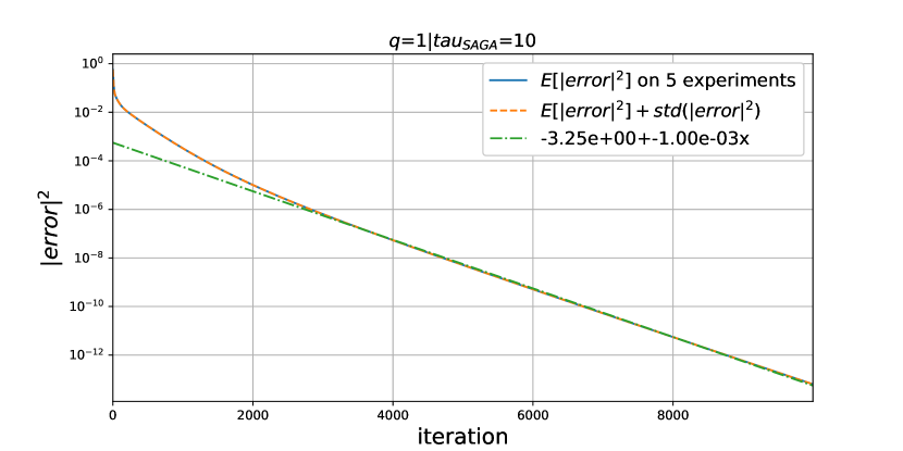
(a) $q=1$

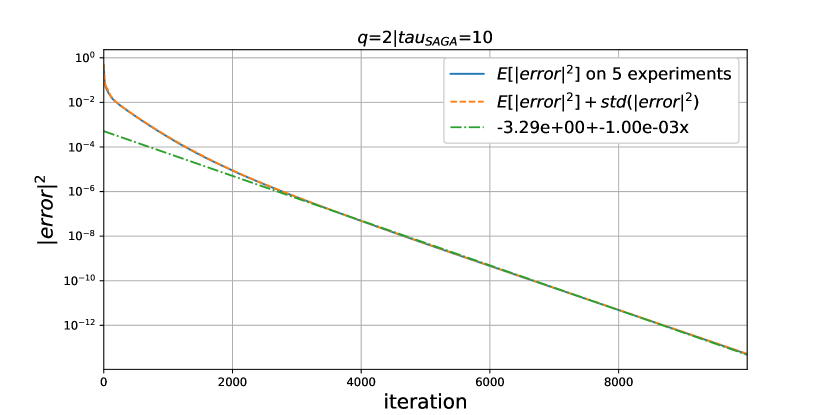
(b) $q=2$

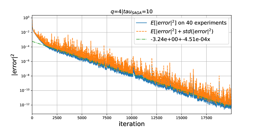
(c) $q=4$

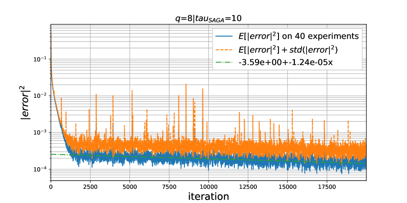
(d) $q=8$

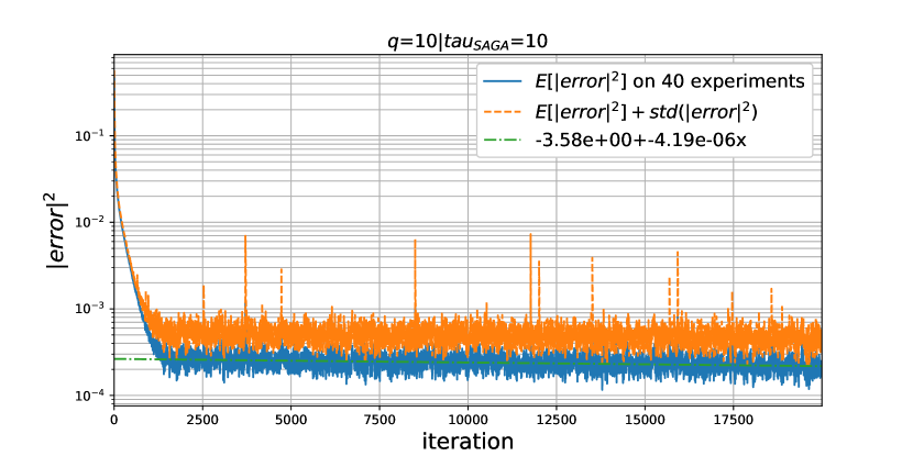
(e) $q=10$

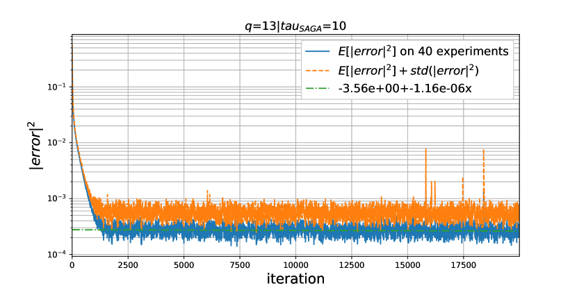
(f) $q=13$

Figure 1: Convergence of SAGA w.r.t. the iteration counter for different $q$ and fixed FE mesh

We show in Figure 1 the convergence plots of $\log(\mathbb{E}[\|error\|])$ versus the number of iterations, for $q\in\{2,4,8,13\}$ and in Figure 2 a zoom on the first $2000$ iterations. We clearly observe two regimes: a first one over the first few hundreds of iterations, of faster exponential convergence, and a second one afterwards, of slower, but still exponential convergence. We assess hereafter that the slower rate observed behaves as predicted by our analysis in Corollary 4.14. We are not able to explain at the moment, however, the faster initial regime.

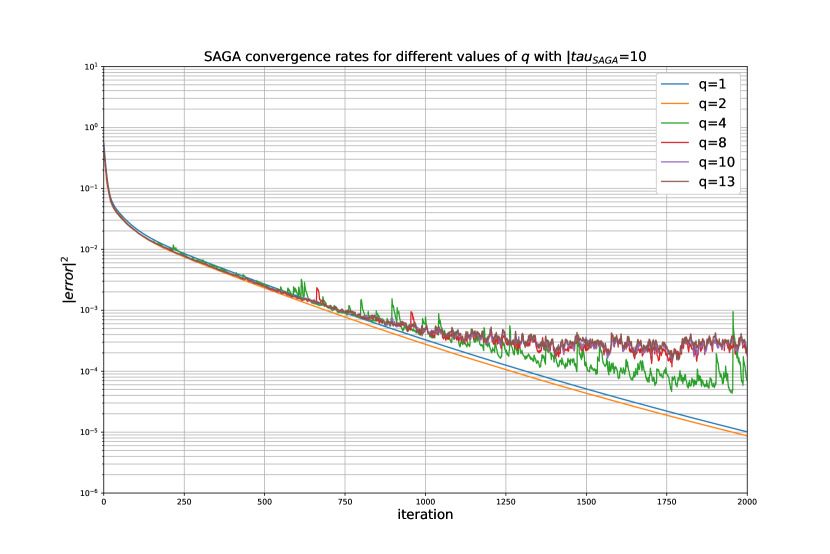
Figure 2: Convergence of SAGA algorithm w.r.t. the iteration counter, for different values of $q$ and fixed FE mesh. Zoom of Figure 1 on the first $2000$ iterations

In order to verify quantitatively the exponential error decay $\widetilde{E_{1}}(1-\epsilon)^{k}$ of equation (48), with $\epsilon\sim\frac{1}{n}$, we have estimated by least squares fit the constant $\widetilde{E_{1}}$ and rate $\epsilon$ for each value of $q$ (we have taken only the second regime into consideration in the least squares fit). In Figure 3(a), we plot the ratio between the estimated convergence rate $\epsilon_{est}$ and the theoretical one $\epsilon_{th}=\frac{1}{2n}=\frac{1}{2q^{5}}$ for the different tested values of $q$. Similarly, in Figure 3(b) we plot the estimated constant $\widetilde{E_{1}}$ versus $q$. estimate the constants but you seem to be using some In both cases, the plotted quantities vary very little with $q\in\{3,\dots,13\}$ which confirms the validity of our theoretical analysis.

(a) $\epsilon_{exp.}/\epsilon_{th}$ versus $q$

(b) Estimated constant $\widetilde{E_{1}}$ versus $q$

Figure 3: Estimation of the SAGA rate $\epsilon$ and constant $\widetilde{E_{1}}$ versus $q$

We analyze next the sensitivity of the SAGA algorithm w.r.t. the step-size $\tau$. In Figure 4, we plot the mean squared error $\mathbb{E}[\|u_{k}-u_{ref}\|^{2}]$ versus the iteration counter, for $q=5$, where the expectation is estimated from $5$ independent experiments. With a large step-size, $\tau=100$, the method diverges to infinity. Progressively decreasing $\tau$ to $10$, the method starts converging, with the expected exponential rate, although slowly. Among the different values that we have tried, a step size $\tau=10$ seems to provide the fastest convergence. Further decreasing $\tau$ to $0.01$ makes SAGA converge poorly.

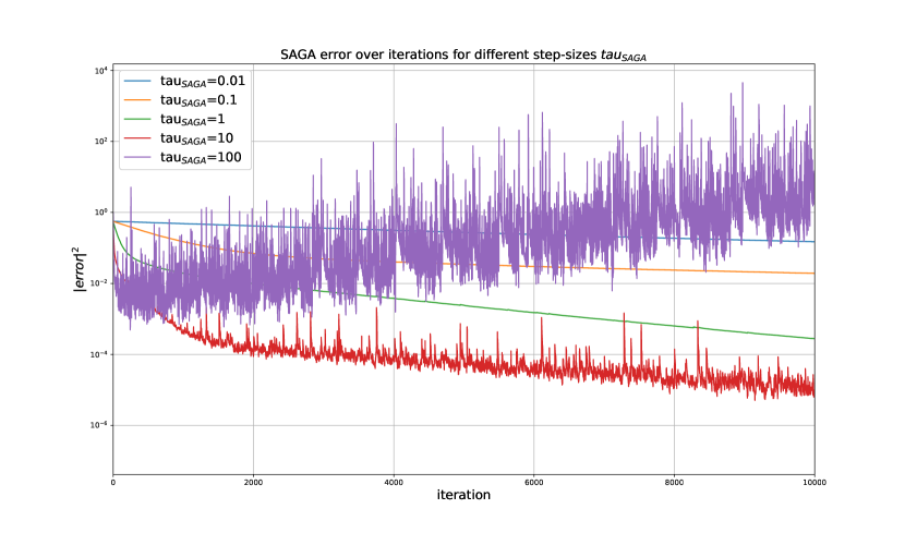
Figure 4: Sensitivity of SAGA (with $q=5$) to the choice of the step size $\tau$.

In Figure 5 we compare the convergence rate of SAGA, with $\tau=10$ with that of CG. The error in both cases is plotted against the total number of PDE solves. The plot shows a faster convergence of CG than SAGA, asymptotically. However, SAGA features a smaller error in the pre-asymptotic regime, and delivers an acceptable solution, from a practical point of view, already before two full iterations of CG (2500 PDE solves). This makes it attractive in a limited budget context.

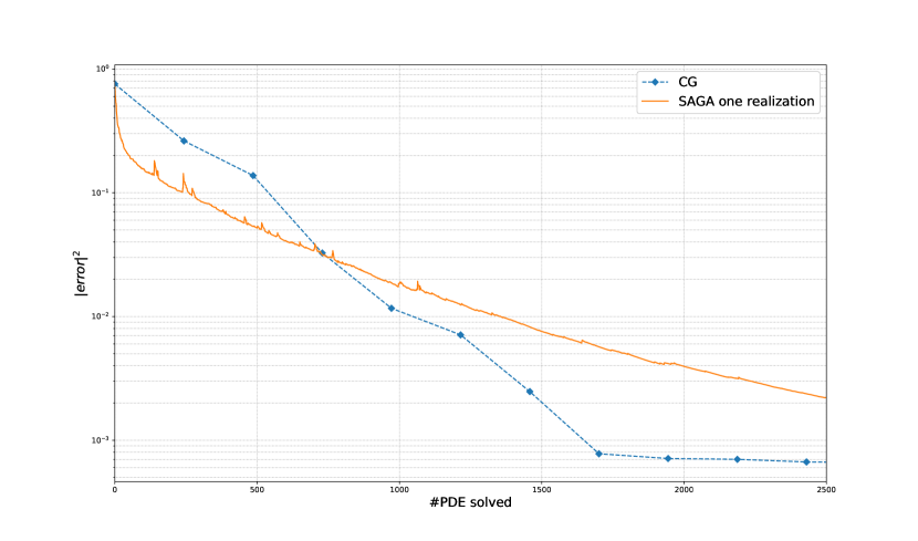
Figure 5: Comparison of SAGA with $\tau=10$ vs CG, for $q=3$, $h=\frac{1}{55}$.

5.2.1 Complexity results for the SAGA algorithm

We investigate here the complexity of the SAGA method (35), for which we recall the error bound (49) in the case of piece-wise linear FE (i.e. $r=1$) and a 5-dimensional probability space (i.e. $M=5$):

(57) $$\mathbb{E}[\|\widehat{u}_{SAGA_{k}}^{h}-u^{*}\|^{2}]\leq\widetilde{E_{1}}(1-\epsilon(q))^{k}+\widetilde{E_{2}}e^{-sq}+\widetilde{E_{3}}h^{4}$$

where $s$ is the rate of exponential convergence of the quadrature formula, and $q$ the number of knots used in each stochastic variable. To assess the complexity of the method and balance the error contributions, we need first to estimate the constants $\widetilde{E_{1}}$, $\widetilde{E_{2}}$, $\widetilde{E_{3}}$ and rates $\epsilon$ and $s$. For this, we have proceeded in the following way:

• Estimation of $\widetilde{E_{1}}$ and $\epsilon=\epsilon(q)$. This has been done already in the previous section using a fixed mesh with $h=2^{-3}$. From Figure 3 we infer the values $\widetilde{E_{1}}\approx 2.95$ and $\epsilon(q)\approx\frac{1.0}{q^{5}}$.

• Estimation of $\widetilde{E_{2}}$ and $s$. We used again a fixed mesh of size $h=2^{-3}$. First, we computed the reference solution with a fine Gauss-Legendre quadrature formula, i.e. $q=8$, using the CG algorithm until convergence. Then we computed the error for the approximated optimal control using only $q\in\{1,\dots,7\}$ points in each random variable, using again the CG algorithm until convergence. Results are detailed in Table 2 and plotted in Figure 6. The error is the difference between the estimated optimal control using $q\in\{1,\dots,7\}$ knots in the quadrature formula, and the optimal control computed for $q=8$. We estimate $\widetilde{E_{2}}\approx 10.43$ and $s\approx 3.697$.

  $q$	$\|error\|^{2}$
  1	3.501974e-03
  2	7.842113e-07
  3	7.583597e-11
  4	6.019157e-15
  5	1.281663e-18
  6	3.673762e-22
  7	7.141313e-25

  Table 2: Quadrature error on the optimal control, versus the number of knots $q$ used in each random variable.

  

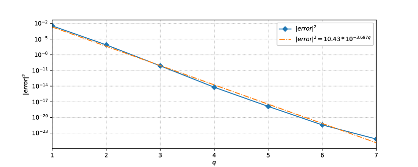
  Figure 6: Fitting the (squared) quadrature error model $\widetilde{E_{2}}e^{-sq}$ in (57).

• Estimation of $\widetilde{E_{3}}$. We used a quadrature formula with $q=1$ knot in each random variable, and computed the reference solution on a fine mesh (with $h=2^{-8}$) using the CG algorithm until convergence. Then we run again the CG algorithm with the same setting, yet on coarser meshes with size $h=2^{-1},\dots,2^{-8}$. The results are shown in Table 3 and Figure 7 which confirm a convergence of order $h^{4}$ of the squared error with an estimated constant $\widetilde{E_{3}}\approx 2.96$.

  $h^{-1}$	$\|error\|^{2}$
  2	1.153577e-01
  4	1.544431e-02
  8	1.068433e-03
  16	7.209996e-05
  32	4.561293e-06
  64	2.824879e-07
  128	1.695013e-08
  256	7.707942e-10

  Table 3: FE error on the optimal control (computed with $q=1$) versus the mesh size $h$.

  

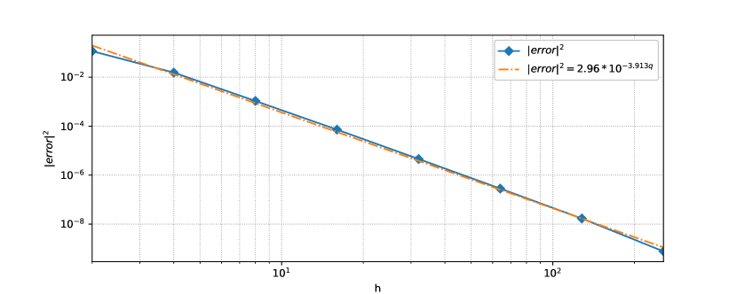
  Figure 7: Fitting the (squared) FE error model $\widetilde{E_{3}}h^{-4}$ in (57).

We are now ready to assess the complexity of the SAGA algorithm. For this, for a given tolerance $tol$, we compute the optimal mesh size $h(tol)$, the optimal number of Gauss-Legendre points in the quadrature formula $q(tol)$, and the optimal number of SAGA iterations $k_{max}(tol)$, using the constants $\widetilde{E_{1}}$, $\widetilde{E_{2}}$ and $\widetilde{E_{3}}$ and rates $\epsilon(q)$ and $s$ estimated above. Then we run the SAGA algorithm up to iteration $k_{max}$, on a mesh of size $h(tol)$, using a quadrature formula with $q(tol)$ points in each random variable, and plot the error on the optimal control for a single realization. The reference solution has been computed using the CG method, on a mesh of size $h=2^{-8}$, with a quadrature formula with $q=5$, until we reach a very small tolerance, ($k_{max}=30$, $\|\nabla J(u_{30})\|\leq 10^{-17}$, $\|u_{30}-u_{29}\|\leq 10^{-13}$) Figure 8 shows the errors of such SAGA simulations versus the computational cost model $W=k_{max}h^{-d}$. Table 4 gives details on the optimal discretization parameters $h,q,k_{max}$ as well as the required complexity for each considered tolerance.

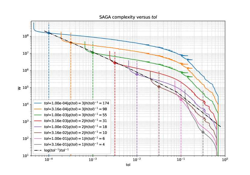
Figure 8: Computational work model versus estimated error for the SAGA method (35). Each curve represents the evolution of the error along the SAGA iterations; the diamond corresponds to the iteration $k_{\text{fst}}$, at which the targeted tolerance is first met. The optimal (theoretical) iteration counter $k_{max}(tol)$ is given for comparison purpose in Table 4.

$tol$	$q(tol)$	$h(tol)^{-1}$	$k_{max}(tol)$	error$(k_{max}(tol))$	$k_{\text{fst}}$	error$({k_{\text{fst}}})$	$W$
3.162e-01	1	4	1124	1.237e-01	15	3.156e-01	2.400e+02
1.000e-01	1	6	1699	7.277e-02	539	9.997e-02	1.940e+04
3.162e-02	2	10	2274	2.017e-02	1111	3.161e-02	1.111e+05
1.000e-02	2	18	2849	6.495e-03	1818	9.997e-03	5.890e+05
3.162e-03	2	31	3424	2.415e-03	2864	3.162e-03	2.752e+06
1.000e-03	3	55	3999	6.611e-04	3620	9.995e-04	1.095e+07
3.162e-04	3	98	4574	1.909e-04	4443	3.160e-04	4.267e+07
1.000e-04	3	174	5149	4.556e-05	5125	9.996e-05	1.552e+08

Table 4: Final error for one realization of SAGA, versus the target tolerance $tol$. $k_{\text{fst}}$ corresponds to the iteration at which the targeted tolerance is first met.

The results follow well the predicted theoretical complexity given in Corollary 4.23, at least for small tolerances.

6 Conclusions

In this work, we have proposed a SAGA algorithm with importance sampling to solve numerically a quadratic optimal control problem for a coercive PDE with random coefficients, minimizing and expected regularized mean squares loss function, where the expectation in the objective functional has been approximated by a quadrature formula whereas the PDE has been discretized by a Galerkin method. The SAGA algorithm is a Stochastic Gradient type algorithm with a fixed-length memory term, which computes at each iteration the gradient of the objective functional in only one quadrature point, randomly chosen from a possibly non-uniform distribution. We have shown that the asymptotically optimal sampling distribution is the uniform one, over the quadrature points. We have also shown that, when equilibrating the three sources of errors, namely the PDE discretization error, the quadrature error and the error due to the SAGA optimization algorithm, the overall complexity, in terms of computational work versus prescribed tolerance, is asymptotically the same as the one of gradient based methods, such as Conjugate gradient (i.e. methods that sweep over all quadrature points at each iteration), as the tolerance goes to zero. However, as illustrated by our numerical experiments, the advantage of SAGA with respect to CG is in the pre-asymptotic regime, as acceptable solutions may be obtained already before a full sweep over all quadrature points is completed. The main limitation we see for this method is the required memory space, since the storage increases as the desired tolerance gets smaller, hence the number of quadrature points increases, and will reach at some point the memory limit of the employed machine. Although we point out that only one “gradient” term has to be updated at each iteration. Therefore, one could also dump all gradients on the hard disk and overwrite only one term per iteration. This will slightly slow down the execution, but performance will still be acceptable as long as the communication/access (a.k.a. Disk I/O) time is negligible compared to the time to solve one PDE.

As a particular example, we have considered a diffusion equation with diffusivity coefficient that depends analytically on a few uniformly distributed and independent random variables. For this problem, we have considered and analyzed a full tensor Gauss-Legendre quadrature formula, which, however, is affected by the curse of dimensionality, hence applicable only to problems for which the randomness can be described in terms of a small number of random variables. To overcome such curse of dimensionality, one could use sparse quadratures instead [1, 10, 2], whose weights, however, are not all positive. The result in Lemma 4.10 is still valid, as long as the approximate functional $\widehat{J}$ satisfies a strong convexity condition,

$$\frac{l}{2}\|u_{1}-u_{2}\|^{2}\leq\langle\nabla\widehat{J}(u_{1})-\nabla\widehat{J}(u_{2}),u_{1}-u_{2}\rangle\quad\forall u_{1},u_{2}\in U,$$

which might hold only for a sufficiently large number of quadrature points (see Remark 4.18). Also, because of the presence of negative weights, the quantity $\widetilde{S}_{n}$ might not be uniformly bounded in $n$, therefore, the results in Theorem 4.12 and Corollary 4.14 might not apply to this case. These issues will be further investigated in a future work. The complexity analysis of the SAGA method presented in Section 4.3 assumed a sub-exponential decay of the quadrature error. Analogous complexity results could be derived under the assumption of an algebraic decay rate of the quadrature error as, for instance, for a MC or QMC quadrature. We should point out, however, that for a MC quadrature formula, the overall complexity will be dominated by the slow $n^{-\frac{1}{2}}$ Monte Carlo convergence rate and SAGA will not improve the complexity of SG, and is therefore not recommended in this case. On the other hand, SAGA gains over SG whenever the quadrature formula has a better convergence rate than MC. This will be the case for a QMC quadrature formula.

References

- [1] I. Babuška, F. Nobile, and R. Tempone, A stochastic collocation method for elliptic partial differential equations with random input data, SIAM review, 52 (2010), pp. 317–355.
- [2] A. Borzì, Multigrid and sparse-grid schemes for elliptic control problems with random coefficients, Computing and Visualization in Science, 13 (2010), pp. 153–160, https://doi.org/10.1007/s00791-010-0134-4.
- [3] A. Chkifa, A. Cohen, and C. Schwab, Breaking the curse of dimensionality in sparse polynomial approximation of parametric pdes, Journal de Mathématiques Pures et Appliquées, 103 (2015), pp. 400 – 428.
- [4] A. Defazio, F. Bach, and S. Lacoste-Julien, Saga: A fast incremental gradient method with support for non-strongly convex composite objectives, in Advances in Neural Information Processing Systems 27, Z. Ghahramani, M. Welling, C. Cortes, N. D. Lawrence, and K. Q. Weinberger, eds., Curran Associates, Inc., 2014, pp. 1646–1654.
- [5] O. G. Ernst, B. Sprungk, and L. Tamellini, Convergence of sparse collocation for functions of countably many Gaussian random variables (with application to elliptic PDEs), SIAM J. Numer. Anal., 56 (2018), pp. 877–905, https://doi.org/10.1137/17M1123079.
- [6] A.-L. Haji-Ali, F. Nobile, L. Tamellini, and R. Tempone, Multi-index stochastic collocation convergence rates for random PDEs with parametric regularity, Found. Comp. Math., 16 (2016), pp. 1555–1605, https://doi.org/10.1007/s10208-016-9327-7.
- [7] F. Hecht, New development in freefem++, J. Numer. Math., 20 (2012), pp. 251–265.
- [8] M. Hinze, R. Pinnau, M. Ulbrich, and S. Ulbrich, Optimization with PDE Constraints, Mathematical Modelling: Theory and Applications 23, Springer, New York, 2009, https://doi.org/10.1007/978-1-4020-8839-1.
- [9] D. P. Kouri and T. M. Surowiec, Existence and optimality conditions for risk-averse PDE-constrained optimization, SIAM/ASA J. Uncertain. Quantif., 6 (2018), pp. 787–815, https://doi.org/10.1137/16M1086613.
- [10] H.-C. Lee and M. D. Gunzburger, Comparison of approaches for random pde optimization problems based on different matching functionals, Computers and Mathematics with Applications, 73 (2017), pp. 1657 – 1672, https://doi.org/10.1016/j.camwa.2017.02.002.
- [11] M. C. Martin, S. Krumscheid, and F. Nobile, Analysis of stochastic gradient methods for PDE-constrained optimal control problems with uncertain parameters, MATHICSE Technical Report 04.2018, École Polytechnique Fédérale de Lausanne, 2018.
- [12] F. Nobile, L. Tamellini, and R. Tempone, Convergence of quasi-optimal sparse grid approximation of Hilbert-space-valued functions: application to random elliptic PDEs, Numer. Math., 134 (2016), pp. 343–388, https://doi.org/10.1007/s00211-015-0773-y.
- [13] H. Robbins and S. Monro, A stochastic approximation method, Ann. Math. Statist., 22 (1951), pp. 400–407, https://doi.org/10.1214/aoms/1177729586.
- [14] C. Schillings and C. Schwab, Sparse, adaptive Smolyak quadratures for Bayesian inverse problems, Inverse Problems, 29 (2013), pp. 065011, 28, https://doi.org/10.1088/0266-5611/29/6/065011.
- [15] M. W. Schmidt, R. Babanezhad, M. O. Ahmed, A. Defazio, A. Clifton, and A. Sarkar, Non-uniform stochastic average gradient method for training conditional random fields, in Proceedings of the Eighteenth International Conference on Artificial Intelligence and Statistics, AISTATS 2015, San Diego, California, USA, May 9-12, 2015.
- [16] M. W. Schmidt, N. L. Roux, and F. R. Bach, Minimizing finite sums with the stochastic average gradient., CoRR, abs/1309.2388 (2013).
- [17] G. Szego, Orthogonal polynomials, vol. 23, American Mathematical Soc., 1939.
- [18] J. Zech, D. Dũng, and C. Schwab, Multilevel approximation of parametric and stochastic PDEs, Math. Models and Methods in Appl. Sci., 29 (2019), pp. 1753–1817.