Relativistic spring-mass system

Abstract

The harmonic oscillator plays a central role in physics describing the dynamics of a wide range of systems close to stable equilibrium points. The nonrelativistic one-dimensional spring-mass system is considered a prototype representative of it. It is usually assumed and galvanized in textbooks that the equation of motion of a relativistic harmonic oscillator is given by the same equation as the nonrelativistic one with the mass $M$, at the tip, multiplied by the relativistic factor $1/(1-v^{2}/c^{2})^{1/2}$. Although the solution of such an equation may depict some physical systems, it does not describe, in general, one-dimensional relativistic spring-mass oscillators under the influence of elastic forces. In recognition to the importance of such a system to physics, we fill a gap in the literature and offer a full relativistic treatment for a system composed of a spring attached to an inertial wall, holding a mass $M$ at the end.

I Introduction

The harmonic oscillator has universal importance to physics, once it describes small oscillations close to stable equilibrium points of general systems. A prototype harmonic oscillator is the nonrelativistic one-dimensional spring-mass system, since the parabolic potential is approximately valid (for a variety of materials) as far as the (small-mass) spring does not suffer plastic deformations. In addition, it has been assumed for long and galvanized in textbooks (see, e.g., Refs. pz ; h ; klml ; gps and references therein) that the motion $x=x(t)$ of a relativistic “harmonic” oscillator would satisfy

$$\frac{d}{dx^{0}}\frac{M\dot{x}}{(1-\dot{x}^{2}/c^{2})^{1/2}}=-\frac{\partial\Phi}{\partial x},$$ (1)

where $M$ is the particle (rest) mass, $c$ is the speed of light, ${}^{\prime}\;\dot{}\;^{\prime}\equiv d/dx^{0}$, $x=x^{1}$, and $x^{\mu}$ are usual inertial Cartesian coordinates covering the Minkowski spacetime $(\mathbb{R}^{4},\eta_{\mu\nu})$ with metric $\eta_{\mu\nu}$ chosen here to have signature $(+,-,-,-)$. The potential corresponding to Hooke’s law would be $\Phi=kx^{2}/2$, where $k$ is the usual elastic constant. Correspondingly, the energy conservation equation would be given by

$$\frac{Mc^{2}}{(1-\dot{x}^{2}/c^{2})^{1/2}}+\Phi\equiv{\cal E}={\rm const}.$$ (2)

It should be stressed, however, that although Eqs. (1) and (2) may describe some physical systems (see Appendix A), they do not characterize one-dimensional relativistic spring-mass oscillators under the influence of elastic forces.

Although some attention has been devoted to the issue of elasticity in the relativistic context bs ; bp , it is somewhat surprising that the relativistic spring-mass system has not received a comprehensive relativistic treatment yet. This may be because the speed of sound $v_{s}$ is typically small under usual conditions, e.g., approximately 13 km/s for beryllium and silicon carbide, 12 km/s for diamond and 10 km/s for aramid (a class of synthetic fiber), while maximum local velocities $v_{m}$ should be even smaller. (As it will be seen further, $v_{m}$ may be estimated by multiplying $v_{s}$ by the maximum strain, i.e., the maximum relative spring deformation.) In spite of the small local velocity rates achieved in most materials under normal conditions, we must recall that this may be radically altered under extreme regimes. In neutron stars, e.g., the sound and light velocities can become comparable.

In view of the importance of harmonic oscillators to physics, we offer here a comprehensive treatment of the relativistic one-dimensional Hookean spring-mass system in Minkowski spacetime. The paper is organized as follows. In Sec. II, we define the spring stress-energy-momentum tensor $T_{ab}$. In Sec. III, we use $T_{ab}$ derived earlier to describe the spring dynamics. In Sec. IV, we impose conditions on the spring to respect causality and show that the equations of motion are hyperbolic if and only if the weak energy condition is satisfied. In Sec. V, we define the boundary conditions and discuss energy conservation. In Secs. VI and VII, we apply our results to discuss the nonrelativistic and relativistic spring-mass systems, respectively. Conclusions are presented in Sec. VIII. We assume units where $c=1$, unless stated otherwise, and metric signature $(+\,-\,-\,-)$.

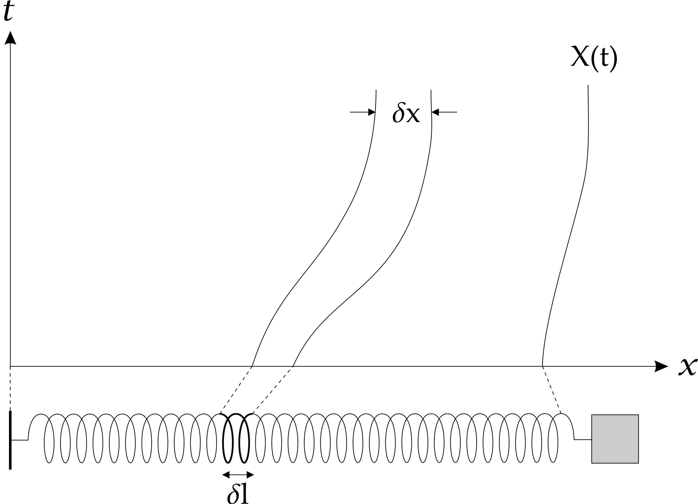
Figure 1: The spring points are labeled by their (relaxed) proper distance $l$ to the wall chosen to lie at rest at the Cartesian coordinate $x^{1}=0$. The Cartesian coordinates of point $l$ at moment $x^{0}\equiv t$ are $x^{1}=x(t,l)$, $x^{2}=x^{3}=0$.

II The stress-energy tensor

Let us consider a one-dimensional spring-mass system in Minkowski spacetime set to oscillate at relativistic velocities. The spring is assumed to be fixed to an infinitely massive inertial wall at one end and to a point mass $M$ at the other one. The relaxed spring mass and proper length will be denoted by $m$ and $L$, respectively. We might feel tempted to neglect the spring mass when $m\ll M$ by imposing $m=0$ from the beginning (as it is usual in Newtonian physics). However, this will be proved illegal as far as one requests the equation of motion to be hyperbolic and the weak energy condition to be satisfied. Furthermore, we shall see that contributions due to the spring mass are typically larger than the ones due to relativistic corrections. Thus, we would rather make no assumptions on $m/M$ (except in Sec. VI, where we expand the equation of motion in terms of $m/M\ll 1$ in order to expose more clearly the physical content of our results).

Our spring will obey Hooke’s law in the sense that the proper force at the tip of the static spring will be $-k(X-L)$, where $k$ is the spring constant and $X$ is the compressed/stretched spring proper length. It is also assumed to be homogeneous: not only it will have constant linear density $\lambda=m/L$ along its length, but if we cut out some portion of it with relaxed proper length $L^{\prime}$, such a portion will behave as a spring with $k^{\prime}=k(L/L^{\prime})$ itself. For the sake of simplicity, our spring will be modeled as a long cylinder with cross sectional area $a$ and vanishing Poisson’s ratio (i.e., $a={\rm const}$ during the motion) in which case the Young’s modulus is $Y\equiv kL/a={\rm const}$.

We cover the Minkowski spacetime with inertial Cartesian coordinates $x^{\mu}$ and set the wall to lie at the origin. We also let the $x^{1}$ axis to be aligned with the spring motion. Each spring point will be labeled by a parameter, $l\in\mathbb{R}$, corresponding to the proper distance between the point and the wall when the spring is relaxed. We denote by $x^{1}=x(t,l)$ the $x^{1}$ coordinate of the point $l$ at time $t$. The coordinates $(t,l)$ are related to the inertial Cartesian coordinates $(x^{0},x^{1})$ by the transformation

$$x^{0}=t,\;\;\;\;\;\;x^{1}=x(t,l).$$ (3)

The position of the mass $M$ attached to the end of the spring (see Fig. 1) is given by $X(t)=x(t,L)$.

In order to derive the equation of motion, we should first determine the spring’s stress-energy tensor $T^{ab}$. Inertial observers instantaneously at rest with respect to some arbitrary spring point $l$ may adapt a local inertial Cartesian coordinate system ${x^{\prime}}^{\mu}=(t^{\prime},x^{\prime},y^{\prime},z^{\prime})$ and define $T\equiv T^{\mu\nu}_{0}\partial/\partial{x^{\prime}}^{\mu}\otimes\partial/\partial{x^{\prime}}^{\nu},$ with

$$T^{\mu\nu}_{0}=\left(\begin{array}[]{cccc}\rho_{0}&0&0&0\\ 0&\tau_{0}&0&0\\ 0&0&0&0\\ 0&0&0&0\end{array}\right),$$ (4)

where $\rho_{0}$ and $\tau_{0}$ are the proper mass density and pressure along the $x$-direction, respectively. We note that the one-dimensional character of the problem, together with the negligible Poisson ratio of the spring should prevent any other tension components to appear in Eq. (4) note1 . We will assume that according to such instantaneously comoving observer, close enough points at $l+\delta l$ move sufficiently slowly to be under the influence of Hooke’s force $F$. (Up to first order in $\partial(\partial x/\partial l)/\partial t$, this assumption is not any stronger than the one required for Newtonian springs.) As a result, we can write $\tau_{0}\equiv F/a=-Y(\gamma\delta x-\delta l)/\delta l$ as

$$\tau_{0}=-Y\left(\gamma\frac{\partial x}{\partial l}-1\right),$$ (5)

where $\delta x\equiv x(t,l+\delta l)-x(t,l)$ and $\gamma\equiv(1-u^{2})^{-1/2}$, with $u\equiv{\partial x(t,l)}/{\partial t}.$ The factor $\gamma$ was introduced to convert the coordinate distance $\delta x$ into proper distance. We recall that because of the spring homogeneity, $Y=kL/a=k^{\prime}\delta l/a$, with $k^{\prime}$ being the spring constant of a relaxed segment with proper size $\delta l$.

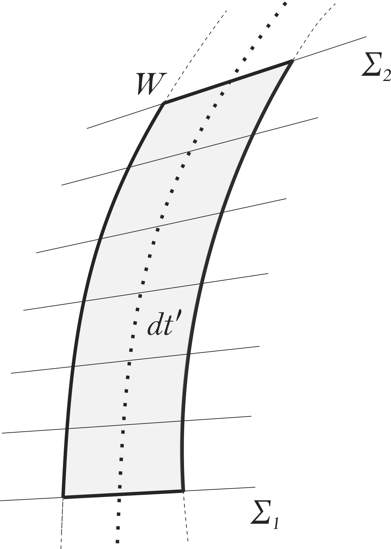
Figure 2: The region $W,$ outlined with bold lines, is the portion of the worldtube of the spring containing the points in the interval $\mathcal{I}=(l,l+\delta l)$. This region is sliced by a family of spacelike hypersurfaces $\Sigma_{t^{\prime}}$ orthogonal to the worldline of some fiducial spring point in the interval and labeled by its proper time $t^{\prime}$.

Since there are no external forces acting on the interior points of the spring, the stress energy tensor satisfies

$$\nabla_{a}T^{ab}=0$$ (6)

for $0<l<L$. This yields two independent equations, which should be solved for $x(t,l)$ and $\rho_{0}(t,l)$. In order to obtain $\rho_{0}$, let us use Stokes’ theorem and Eq. (6) to write

$$\int_{W}T^{ab}\nabla_{a}U_{b}\,d\Xi=\int_{\partial W}T^{ab}U_{b}\,d\Sigma_{a}.$$ (7)

Here, $U^{a}$ is the 4-velocity vector field of the spring points, $W$ is the spacetime region defined by the worldlines in the interval $\mathcal{I}\equiv(l,l+\delta l)$ and delimited by the past, $\Sigma_{1}$, and future, $\Sigma_{2}$, spacelike hypersurfaces, $\partial W$ denotes the boundary of $W$, $d\Xi$ is the spacetime volume element, and $d\Sigma^{a}$ is the vector-valued volume element induced on $\partial W$ (see Fig. 2). Since there is no flux of momentum seen by an observer accompanying the matter flow, we can cast Eq. (7) as

$$\delta m_{2}-\delta m_{1}=\int_{W}T^{ab}\nabla_{a}U_{b}\,d\Xi,$$ (8)

where

$$\delta m_{j}\equiv(-1)^{j}\int_{\Sigma_{j}}T^{ab}U_{b}\,d\Sigma_{a},\;\;j=1,2,$$ (9)

is the proper mass of the piece $\mathcal{I}$ of the spring at $\Sigma_{j}$. (The factor $(-1)^{j}$ appears only to fix the orientation of $d\Sigma^{a}$ introduced in Eq. (7), which is past directed on $\Sigma_{1}$.)

In order to evaluate the right-hand side of Eq. (8), we will first choose some fiducial worldline associated with a point within the the portion $\mathcal{I}$ of the spring. Then, we will partition the region $W$ into infinitesimal cells by slicing it with spacelike hypersurfaces $\Sigma_{t^{\prime}}$ (with $\Sigma_{t^{\prime}_{1}}\equiv\Sigma_{1}$ and $\Sigma_{t^{\prime}_{2}}\equiv\Sigma_{2}$) differing by an infinitesimal proper time $dt^{\prime}$ and which are orthogonal to the fiducial worldline, as it is shown in Fig. 2. Hence, we can write

$$\int_{W}T^{ab}\nabla_{a}U_{b}\,d\Xi=\int_{t^{\prime}_{1}}^{t^{\prime}_{2}}dt^{\prime}\int_{\Sigma_{t^{\prime}}}dx^{\prime}dy^{\prime}dz^{\prime}T^{ab}\nabla_{a}U_{b}.$$ (10)

Here, $(t^{\prime},x^{\prime},y^{\prime},z^{\prime})$ are local inertial Cartesian coordinates associated, within each cell, with the fiducial worldline. In these coordinates, the components of $T^{ab}$ are given by $T^{\mu\nu}_{0}$ in Eq. (4) and $U^{a}$ decomposes as $U^{\mu}=\gamma^{\prime}(1,\vec{u}\,^{\prime})$, the prime indicating velocities with respect to the local inertial frame being used. As a consequence, $u^{\prime}\ll 1$, $\gamma^{\prime}\approx 1$, and

$$T^{ab}\nabla_{a}U_{b}=T^{00}_{0}\partial U_{0}/\partial t^{\prime}+T^{11}_{0}\partial U_{1}/\partial x^{\prime}\approx-\tau_{0}\frac{\partial{u^{\prime}}^{1}}{\partial x^{\prime}},$$ (11)

with the approximation becoming exact as $\delta l\rightarrow 0$. Now, if we use Eq. (11) together with the identity

$$\frac{d}{dt^{\prime}}\delta V^{\prime}=(\nabla\cdot\vec{u}^{\prime})\delta V^{\prime},$$ (12)

where $\delta V^{\prime}\equiv a\delta x^{\prime}$ and $\delta x^{\prime}$ is the length of the piece of the spring as measured in the local inertial frame, we can cast Eq. (10) as

$$\int_{W}T^{ab}\nabla_{a}U_{b}\,d\Xi=-\int_{t^{\prime}_{1}}^{t^{\prime}_{2}}dt^{\prime}a\tau_{0}\frac{d(\delta x^{\prime})}{dt^{\prime}},$$ (13)

where $\int_{\Sigma_{t^{\prime}}}$ was suppressed once we are looking at a spring element. By making use of the above result in Eq. (8), we find that the change in the proper mass of the piece of the spring as it evolves from $\Sigma_{1}$ to $\Sigma_{2}$ is

$$\delta m_{2}-\delta m_{1}=-\int_{t^{\prime}_{1}}^{t^{\prime}_{2}}dt^{\prime}a\tau_{0}\frac{d(\delta x^{\prime})}{dt^{\prime}}=-\int_{\delta x^{\prime}_{1}}^{\delta x^{\prime}_{2}}a\tau_{0}d(\delta x^{\prime}).$$ (14)

Consequently, we conclude that any change in the mass of the portion $\mathcal{I}$ of the spring is due to the total work done on it by the neighboring matter. Using Hooke’s law (5) and integrating from the moment the piece is relaxed, where $\delta x^{\prime}_{1}=\delta l$ and $\delta m_{1}=\lambda\delta l$, to some arbitrarily time in the wall’s frame, where $\delta x^{\prime}_{2}=\gamma\delta x$, we find that

$$\delta m_{2}-\lambda\delta l = \frac{aY}{\delta l}\int_{\delta l}^{\gamma\delta x}(\delta x^{\prime}-\delta l)d(\delta x^{\prime})$$ (15)

$$= \frac{aY}{2\delta l}(\gamma\delta x-\delta l)^{2}$$

and hence,

$$\delta m_{2}-\lambda\delta l=\frac{aY\delta l}{2}{\left(\gamma\frac{\partial x}{\partial l}-1\right)}^{2}.$$ (16)

By making use of Eq. (16), it is possible to write the proper mass density $\rho_{0}\equiv\delta m_{2}/(a\gamma\delta x)$ in terms of $x(t,l)$ as

$$\rho_{0}=\frac{\lambda}{a}{\left(\gamma\frac{\partial x}{\partial l}\right)\!}^{-1}+\frac{Y}{2}{\left(\gamma\frac{\partial x}{\partial l}\right)\!}^{-1}{\left(\gamma\frac{\partial x}{\partial l}-1\right)}^{2}.$$ (17)

To find the components, $T^{\mu\nu}$, of the stress-energy tensor in the frame of the wall, we can simply apply a boost with velocity $(-u,0,0)$ on $T^{\mu\nu}_{0}$ to find that

$$T^{\mu\nu}=\left(\begin{array}[]{cccc}\rho&g&0&0\\ g&p&0&0\\ 0&0&0&0\\ 0&0&0&0\end{array}\right),$$ (18)

where

$$\rho=\gamma^{2}(\rho_{0}+u^{2}\tau_{0}),$$ (19)

$$g=u\gamma^{2}(\rho_{0}+\tau_{0}),$$ (20)

and

$$p=\gamma^{2}(u^{2}\rho_{0}+\tau_{0}),$$ (21)

with $\tau_{0}$ and $\rho_{0}$ being given by Eqs. (5) and (17), respectively. Hence, we have written the spring’s stress-energy tensor entirely in terms of the function $x(t,l)$ (and its derivatives), which describes the configuration of the spring’s points at each time.

III Spring dynamics

We want to find now the equation describing the dynamics of $x(t,l)$. For this purpose, we will first apply Eq. (18) into Eq. (6) in order to obtain

$$\frac{\partial\rho}{\partial x^{0}}+\frac{\partial g}{\partial x^{1}}=0$$ (22)

and

$$\frac{\partial g}{\partial x^{0}}+\frac{\partial p}{\partial x^{1}}=0.$$ (23)

As we have seen in Sec II, the quantities $\rho,$ $g$, and $p$ can be written in terms of $x(t,l)$ and, therefore, it will be more convenient to rewrite Eqs. (22) and (23) using the derivatives $\partial/\partial t$ and $\partial/\partial l$. This can be done by making use of the coordinate transformation (3) to write

$$\frac{\partial}{\partial x^{0}} = -\frac{\partial x}{\partial t}{\left(\frac{\partial x}{\partial l}\right)\!}^{-1}\frac{\partial}{\partial l}+\frac{\partial}{\partial t},$$ (24)

$$\frac{\partial}{\partial x} = {\left(\frac{\partial x}{\partial l}\right)\!}^{-1}\frac{\partial}{\partial l}.$$ (25)

As a result, Eqs. (22) and (23) transform into

$$\frac{\partial x}{\partial l}\frac{\partial\rho}{\partial t}-u\frac{\partial\rho}{\partial l}+\frac{\partial g}{\partial l}=0$$ (26)

and

$$\frac{\partial x}{\partial l}\frac{\partial g}{\partial t}-u\frac{\partial g}{\partial l}+\frac{\partial p}{\partial l}=0,$$ (27)

respectively. By using the explicit expressions for $\rho$, $g$, and $p$ in terms of $x(t,l)$, given by Eqs. (19)-(21) together with Eqs. (5) and (17), we find that Eq. (26) is simply Eq. (27) multiplied by $u=\partial x/\partial t$. Hence, the only relevant equation obtained for $x(t,l)$ is

$$\zeta[x(t,l)]\frac{\partial^{2}x}{\partial t^{2}}-\gamma^{-2}\frac{\partial^{2}x}{\partial l^{2}}-2\frac{\partial x}{\partial t}\frac{\partial x}{\partial l}\frac{\partial^{2}x}{\partial l\partial t}=0,$$ (28)

where

$$\zeta[x(t,l)]\equiv\frac{\lambda}{kL}+\frac{1}{2}-\gamma^{2}\left(\frac{1}{2}+{\left(\frac{\partial x}{\partial t}\right)}^{2}\right){\left(\frac{\partial x}{\partial l}\right)}^{2}$$ (29)

and we recall that $\gamma=(1-({\partial x}/{\partial t})^{2})^{-1/2}.$ The spring dynamics is governed by Eq. (28). In the next section, we shall analyze when it determines the spring evolution once initial (at $t=0$) and boundary (at $l=0$ and $l=L$) conditions are given.

IV Causality, hyperbolicity, and the weak energy condition

The spring equation, Eq. (28), is a quasi-linear second order partial differential equation. As a result, its classification in hyperbolic, parabolic, or elliptic depends on the solution: one needs to take a particular solution $x(t,l)$, insert it into the coefficients of the second order derivatives and then classify it as a linear equation. This corresponds to the evaluation of the sign of the quantity

$$\Delta\equiv\gamma^{4}u^{2}s^{2}+\gamma^{2}\zeta[x(t,l)],$$ (30)

where $s\equiv{\partial x}/{\partial l}$. With the aid of Eq. (29), Eq. (30) can be cast as

$$\Delta=\gamma^{2}\left[\frac{\lambda}{kL}+\frac{1}{2}\left(1-(\gamma s)^{2}\right)\right].$$ (31)

For $\Delta>0$, $\Delta=0,$ and $\Delta<0$, the equation is classified as hyperbolic, parabolic, and elliptic, respectively.

It turns out that this classification is related with the weak energy condition, which ensures that no observer can measure a negative energy density. (It is interesting to note that the weak- and strong-energy conditions are equivalent in the present case.) For the stress-energy tensor given in Eq. (4), this condition translates into

$$\rho_{0}+\tau_{0}>0\>\>\Leftrightarrow\>\>\frac{\lambda}{kL}+\frac{1}{2}\left(1-(\gamma s)^{2}\right)>0.$$ (32)

As a result, the compliance with the weak energy condition is equivalent to the equation being hyperbolic (in the whole domain). It is interesting to note that in order to comply with causality, one must not assume $\lambda=0$ to model light springs; otherwise, Eq. (32) would be violated whenever the spring is stretched, i.e. , $\gamma s>1$.

Although the weak energy condition ensures that the differential equation describing the spring dynamics has a hyperbolic character, which implies that information travels at finite speeds, it does not require such speeds to be smaller than the speed of light. For this to be the case, we need to further constrain the properties of the elastic material composing the spring. This is done by analyzing the characteristic curves of Eq. (28), as they are responsible for propagating the information about the initial data. By using $u=\partial x/\partial t$ and $s=\partial x/\partial l$, Eq. (28) can be rewritten as a first-order quasilinear system when supplemented with the condition $\partial u/\partial l=\partial s/\partial t$. Then, by using standard methods, we find that the slopes (velocities) of the characteristic curves $\left(t,l(t)\right)$ in $(t,l)$ coordinates are given by

$$\nu\equiv\frac{dl}{dt}=\pm\frac{1}{\gamma}\frac{1}{\sqrt{{\lambda}/{(kL)}+\left(1-\gamma^{2}s^{2}\right)/2}\pm\gamma us}.$$ (33)

By transforming to the inertial frame $(x^{0},x^{1})$ using Eq. (3), we find that the speed of the characteristics transforms to

$$\tilde{\nu}\equiv dx(t,l(t))/dt=\nu s+u,$$ (34)

which, by using Eq. (33), can be written as

$$\tilde{\nu}=\pm\frac{1}{\gamma}\frac{s}{\sqrt{{\lambda}/{(kL)}+\left(1-\gamma^{2}s^{2}\right)/2}\pm\gamma us}+u.$$ (35)

We note that there is an asymmetry in the speed of the characteristic curves due to the motion of the points of the spring. To impose that the information travels at speeds smaller than the speed of light, it suffices to ensure this in some arbitrary inertial frame due to the relativistic invariance of Eq. (28). Hence, for each point of the spring, let us take its instantaneous rest frame and put $u=0$ to obtain

$$\tilde{\nu}=\pm\frac{s}{\sqrt{{\lambda}/{(kL)}+\left(1-s^{2}\right)/2}}.$$ (36)

By demanding $|\tilde{\nu}|\leq 1$, we find

$$\frac{\lambda}{kL}-\frac{3s^{2}-1}{2}\geq 0$$ (37)

which constrains the spring (or elastic material) parameters not allowing $\lambda/kL$ to be smaller than some quantity that depends on the instantaneous local deformation of the spring, $s=\partial x/\partial l$. We note that the weak energy condition is automatically satisfied once inequality (37) is respected, as can be seen from Eq. (32) with $\gamma=1$. It is also interesting to note that the weak energy condition supplied by $\lambda/(kL)>(-1/2)(1-s^{2})+2s(1-s)$ implies the dominant energy condition. The dominant energy condition is neither implied nor implies causality.

V Initial and boundary conditions

The initial conditions are determined by giving the position and velocity of each spring point at $t=0$. Hence, given two smooth real functions $q(l)$ and $v(l)$ noteic , we have

$$x(0,l)=q(l)$$ (38)

and

$$\frac{\partial x}{\partial t}(0,l)=v(l).$$ (39)

Let us suppose that at $l=0$ the spring is fixed at a massive wall. Then, $x(t,l)$ satisfies the boundary condition

$$x(t,0)=0$$ (40)

for any $t\in\mathbb{R}_{+}.$ We will restrict attention to initial conditions that respect the above boundary condition. As a result, $q(l)$ and $v(l)$ will satisfy

$$q(0)=0$$ (41)

and

$$v(0)=0.$$ (42)

The attached body, which has been overlooked until now, enters as a boundary condition at $l=L$. The portion of the spring at $l=L$ applies a 3-force $a\tau_{0}$ to the body and since a boost in the direction of the force does not change it, this is precisely the 3-force acting on the mass in the wall’s frame. Therefore, we can write

$$\frac{d}{dt}\left(\Gamma M\frac{dX}{dt}\right)=a\tau_{0},$$ (43)

where $\Gamma(t)\equiv[1-{\left({dX}/{dt}\right)}^{2}]^{-1/2}$ and $X(t)=x(t,L)$. By using Eq. (5) and that $Y=kL/a$, we end up with the equation

$$\frac{d}{dt}\left(\Gamma\frac{dX}{dt}\right)+\frac{kL}{M}\left(\Gamma\left.\frac{\partial x}{\partial l}\right|_{(t,L)}-1\right)=0.$$ (44)

This is a more intricate form of boundary condition as it is also a differential equation and should be solved simultaneously with the spring equation (28).

The local energy conservation given by Eq. (6), together with the fact that the spring is in Minkowski spacetime, ensures us that we can define a conserved energy in any global inertial frame. The wall’s frame is particularly interesting as the wall is static and, hence, it does no work on the spring. To find the conserved energy, let us integrate Eq. (22) with respect to $x$ along the whole spring [i.e., from $0$ to $X(t),$ where we are considering Eq. (3)],

$$\int_{0}^{X(t)}dx\left(\frac{\partial\rho}{\partial t}+\frac{\partial g}{\partial x}\right)=0,$$ (45)

to obtain

$$\frac{d}{dt}\int_{0}^{X(t)}dx\rho(t,x)-\frac{dX}{dt}\rho(t,X(t))+g(t,X(t))-g(t,0)=0.$$ (46)

By using Eqs. (19) and (20) together with boundary condition (40), we find that $g-u\rho=u\tau_{0}$ and $g(t,0)=0$. Hence, we can cast Eq. (46) as

$$\frac{d}{dt}\int_{0}^{X(t)}dxa\rho(t,x)+Ua\tau_{0}(t,X(t))=0,$$ (47)

where $U\equiv dX/dt$. Using the boundary condition (43) at $l=L$, the above equation can be rewritten as

$$\frac{d}{dt}\int_{0}^{X(t)}dxa\rho(t,x)+U\frac{d}{dt}\left(M\Gamma U\right)=0,$$ (48)

which can be easily manipulated to yield

$$\frac{d}{dt}\left[\int_{0}^{X(t)}dxa\rho(t,x)+\Gamma(t)M\right]=0.$$ (49)

As a result, we obtain the conserved energy

$${\cal E}\equiv\int_{0}^{X(t)}dx\,a\rho(t,x)+\Gamma(t)M,$$ (50)

which is exactly the sum of the energies of the spring and of the body in the wall’s frame.

VI The nonrelativistic regime

In order to disentangle the relativistic effects from the nonrelativistic ones, in this section we analyze the nonrelativistic spring-mass system when the spring is massive. Then, in the next section, we will study the relativistic effects by adding the relativistic corrections to the nonrelativistic solution.

In the nonrelativistic regime, where $u=\partial x/\partial t\ll 1$, Eq. (28) reduces to

$$\frac{1}{\vartheta^{2}}\frac{\partial^{2}x}{\partial t^{2}}-\frac{\partial^{2}x}{\partial l^{2}}=0,$$ (51)

where

$$\vartheta\equiv\sqrt{kL/\lambda}$$ (52)

gives the speed of the perturbations of the above wave equation. In the nonrelativistic limit, the boundary conditions (40) and (44) reduce to

$$x(t,0)=0$$ (53)

and

$$\frac{d^{2}X}{dt^{2}}+\frac{kL}{M}\left(\left.\frac{\partial x}{\partial l}\right|_{(t,L)}-1\right)=0,$$ (54)

respectively.

In the remaining of this section, we will first present a procedure to find a general solution of Eq. (51)–with boundary conditions (53) and (54)–in terms of the initial conditions (38) and (39). As it will be discussed, the general solution is not suitable to analyze the light-spring case ($m\equiv\lambda L\ll M$) for arbitrarily large times. Therefore, we will proceed to show how we can evade this problem to find the motion of the (light) spring and determine how its mass affects the motion of the attached body.

VI.1 General solution

The general solution Eq. (51) can written as

$$x(t,l)=f(\vartheta t+l)+h(\vartheta t-l)$$ (55)

where $f$ and $h$ are two arbitrary smooth functions. Imposing the boundary condition (53) at $l=0$ we find that $h=-f$ and thus

$$x(t,l)=f(\vartheta t+l)-f(\vartheta t-l).$$ (56)

By using the initial conditions (38) and (39) at $t=0$, the function $f(z)$, for $z\in[-L,L],$ is determined to be

$$f(z)=\left\{\begin{array}[]{ll}\left(q(z)+{\vartheta}^{-1}\int^{z}_{0}dz^{\prime}v(z^{\prime})\right)/2&\mbox{for $z\in[0,L]$}\\ \left(-q(-z)+{\vartheta}^{-1}\int^{-z}_{0}dz^{\prime}v(z^{\prime})\right)/2&\mbox{for $z\in[-L,0]$}\end{array}\right.,$$ (57)

with which we find $x(t,l)$ for $t\geq 0,$ $l\geq 0$ and $\vartheta t+l\leq L$. Note that a point near the wall does not know about the existence of the body until $t\approx L/\vartheta$, which is the time needed for the information to travel from the body, at $l=L$, to $l\approx 0$.

To determine the motion of the body attached to the spring we need to insert Eq. (56) into the boundary condition (54). This gives

$$f^{\prime\prime}(\vartheta t+L)-f^{\prime\prime}(\vartheta t-L)=\frac{\lambda}{M}\left[1-f^{\prime}(\vartheta t+L)-f^{\prime}(\vartheta t-L)\right],$$ (58)

where the primes indicate derivatives with respect to the argument. By defining $z\equiv\vartheta t+L$ we can rewrite the above equation as

$$f^{\prime\prime}(z)+\frac{\lambda}{M}f^{\prime}(z)=f^{\prime\prime}(z-2L)-\frac{\lambda}{M}f^{\prime}(z-2L)+\frac{\lambda}{M},$$ (59)

with which we are able do extend the function $f$ to the domain $[L,3L]$. In order to see this, note that whenever $z\in[L,3L]$ the right-hand side of Eq. (59) depends only on the values of $f$ and its derivatives in the domain $[-L,L]$, which have already been determined by the initial conditions. Hence, we can take $f(L)$ and $f^{\prime}(L)$ as the initial conditions for Eq. (59) and integrate it from $z=L$ to some $z\in[L,3L]$ to obtain

$$f(z)=f(L)+\left(f(-L)+\frac{M}{\lambda}[f^{\prime}(L)-f^{\prime}(-L)]\right)$$

$$\times\left(1-e^{-{\lambda(z-L)}/{M}}\right)+\int_{L}^{z}dz^{\prime}e^{-{\lambda(z-z^{\prime})}/{M}}$$

$$\times\left(f^{\prime}(z^{\prime}-2L)+\frac{\lambda}{M}[z^{\prime}-L-f(z^{\prime}-2L)]\right).$$ (60)

Similarly, we can extend $f$ to the region $[-3L,-L]$ by rewriting Eq. (58) in terms of $\tilde{z}\equiv\vartheta t-L$ and using $f(-L)$ and $f^{\prime}(-L)$ as its initial conditions when integrating it backwards from $z=-L$ to some $z\in[-3L,-L]$. This process can be repeated indefinitely so that at the $N$-th step $f$ is known in the domain $[-(2N+1)L,(2N+1)L]$, which exactly determines the motion of the body up to some time $t_{N}=2NL/\vartheta$.

However, it is difficult to write down an expression for $f$ in terms of a general $N$, making this kind of solution only useful if we are interested in determining the motion of the body for short times. Although such a method will be useful when analyzing the relativistic corrections to nonrelativistic motion of the spring-mass system, it is unsuitable to the analysis of the light spring, $m=\lambda L\ll M,$ even nonrelativistically. This is due to the fact that, in this limit, $\vartheta$ gets very large and many steps will be needed to determine the motion of the body up to a reasonable time. For instance, consider the angular frequency for the ideal (massless) spring, $\omega_{0}\equiv\sqrt{k/M}$, and take it as the approximate frequency for the light spring case. After a time $t_{1}=2L/\vartheta$ the phase will have changed by

$$\Delta\phi\approx\omega_{0}t_{1}=2L\sqrt{\frac{k}{M}}\sqrt{\frac{\lambda}{kL}}=2\sqrt{\frac{m}{M}}\ll 2\pi,$$ (61)

meaning that $N$ has to be of the order $\sqrt{M/m}$ for one to determine just one cycle of oscillation. Next, we will see how this problem can be circumvented and we will find the first correction coming from the spring mass to the usual harmonic motion of the mass $M$.

VI.2 The harmonic oscillator case and the first correction from the spring mass

For a massless spring, $\lambda=0$, the only admissible configuration is the one in which the spring is homogeneously deformed, i.e., each portion of the spring is deformed by the same ratio. This can be seen directly from Eq. (51), whose solution in this case will be

$$x^{\rm H}(t,l)=a^{\rm H}(t)l,$$ (62)

where we have already imposed the boundary condition (53) at $l=0$. Inserting this solution into Eq. (54) renders the usual equation for the harmonic oscillator (apart from the inhomogeneity that comes from the choice of the spatial coordinate origin at the wall):

$$\frac{d^{2}a^{\rm H}}{dt^{2}}+\omega_{0}^{2}(a^{\rm H}-1)=0,$$ (63)

where we recall that

$$\omega_{0}=\sqrt{\frac{k}{M}}.$$ (64)

The solution of Eq. (63) is the usual harmonic oscillating one, which allows us to write $x^{\rm H}(t,l)$ as

$$x^{\rm H}(t,l)=l\left(1+\frac{A}{L}\cos{(\omega_{0}t+\varphi)}\right)$$ (65)

for arbitrary real constants $A$ and $\varphi$. As a result, the motion of the attached body is described by the well known behavior:

$$X^{\rm H}(t)=L+A\cos{(\omega_{0}t+\varphi)}.$$ (66)

As we have already shown, however, a massless spring is unphysical in the relativistic regime since it violates the weak energy condition. Furthermore, we are going to see that the first relativistic correction over the Newtonian solution is generally smaller than the spring’s mass correction over a massless spring. Thus, it is essential to study the effects of the spring mass on the motion of the attached body. In what follows we will make the assumption that the spring mass is much smaller than the mass of the body, i.e., $m\ll M$. Additionally, to simplify the comparison between the nonrelativistic and relativistic corrections, we will analyze the special case where all the spring points oscillate harmonically with the same frequency $\omega$. (In Appendix B, we analize the case where the mass is stretched and released from rest and obtain similar results.)

Therefore, we will look for solutions of Eq. (51) of the form

$$x(t,l)=b(l)\cos{(\omega t)}+c(l),$$ (67)

with $b$ and $c$ being smooth functions defined on the domain $\left[0,L\right]$ satisfying

$$b(0)=c(0)=0$$ (68)

and

$$\left(\omega_{0}^{2}L\left.\frac{db}{dl}\right|_{l=L}-\omega^{2}b(L)\right)\cos{(\omega t)}=-\omega_{0}^{2}L\left(\left.\frac{dc}{dl}\right|_{l=L}-1\right)$$ (69)

due to the boundary conditions (53) and (54), respectively. Using Eq. (67) in Eq. (51) gives

$$\left(\frac{\omega^{2}}{\vartheta^{2}}b+\frac{d^{2}b}{dl^{2}}\right)\cos{(\omega t)}+\frac{d^{2}c}{dl^{2}}=0,$$ (70)

which implies that

$$b(l)=A\frac{\sin{(\chi l)}}{\sin{(\chi L)}}$$ (71)

and

$$c(l)=Bl,$$ (72)

with $A,B\in\mathbb{R}$ and $\chi\equiv\omega/\vartheta$. Here, we have already imposed the boundary condition (68) on both $b$ and $c$. Now, by using Eqs. (71) and (72) in the boundary condition (69), we arrive at:

$$A\left[\omega_{0}^{2}\chi L\cot{(\chi L)}-\omega^{2}\right]\cos{(\omega t)}+\omega_{0}^{2}L\left[B-1\right]=0,$$ (73)

from which we obtain that $B=1$ and

$$\chi L=\frac{m}{M}\cot{\!\left(\chi L\right)}.$$ (74)

This is a transcendental equation for $\chi$ and its solutions, $\chi_{n}$, can be labeled by nonzero integer index $n$ arranged such that

$$\ldots<\chi_{-2}<\chi_{-1}<0<\chi_{1}<\chi_{2}<\ldots$$

and $\chi_{-n}=-\chi_{n}$. Hence, for each $\omega_{n}=\chi_{n}\vartheta$ satisfying Eq. (74), we have that the corresponding solution $x(t,l)$ is given by

$$x(t,l)=l+A\frac{\sin{(\omega_{n}l/\vartheta)}}{\sin{(\omega_{n}L/\vartheta)}}\cos{(\omega_{n}t)},$$ (75)

which implies that the motion of the attached body is simply

$$X(t)=L+A\cos{(\omega_{n}t)}.$$ (76)

Note that this is still a harmonic motion but now with a frequency $\omega_{n}$ instead of $\omega_{0}$.

From Eq. (74) we can see that, when $m/M\ll 1$, $\chi_{1}L\ll 1$ and $\chi_{n+1}L\approx n\pi$. Hence, to lowest order, i.e., $\tan{\chi_{1}L}\approx\chi_{1}L$, we find that $\chi_{1}L\approx\sqrt{m/M}$ which gives $\omega_{1}\approx\omega_{0}$. Approximating the corresponding solution $x(t,l)$ also to the lowest order we find that

$$x(t,l) = l+A\frac{\sin{(\omega_{1}l/\vartheta)}}{\sin{(\omega_{1}L/\vartheta)}}\cos{(\omega_{1}t)}$$ (77)

$$\approx l\left(1+\frac{A}{L}\cos{(\omega_{0}t)}\right).$$

As a result, the motion of the body is given by

$$X(t)=L+A\cos{(\omega_{0}t)},$$ (78)

which is exactly the solution for the massless spring.

In order to find the spring’s mass correction over the massless spring solution, we will need to go to the next order in the Taylor expansion of $\tan(\chi_{1}L)$. Hence, we write $\tan(\chi_{1}L)\approx(\chi_{1}L)+(\chi_{1}L)^{3}/3$ and use it in Eq. (74) yielding

$$\frac{1}{3}(\chi_{1}L)^{4}+(\chi_{1}L)^{2}-\frac{m}{M}\approx 0,$$ (79)

which gives, up to order $m^{2}/M^{2}$,

$$(\chi_{1}L)^{2}\approx\frac{m}{M}-\frac{1}{3}\frac{m^{2}}{M^{2}}.$$ (80)

As a result, we find that $\omega_{1}=\chi_{1}/\vartheta$ is

$$\omega_{1}\approx\omega_{0}\left(1-\frac{1}{6}\frac{m}{M}\right).$$ (81)

The solution $x(t,l)$, approximated to first order in $m/M$, becomes:

$$x(t,l) = l+A\frac{\sin{(\omega_{1}l/\vartheta)}}{\sin{(\omega_{1}L/\vartheta)}}\cos{(\omega_{1}t)}$$

$$\approx \!\!\!l+A\frac{l}{L}\left[1+\frac{m}{6M}\left(1-\frac{l^{2}}{L^{2}}\right)\right]\cos{\left[\omega_{0}\left(1-\frac{m}{6M}\right)t\right]},$$

from which we find that the motion of the attached body is given by

$$X(t) = L+A\cos{\left[\omega_{0}\left(1-\frac{m}{6M}\right)t\right]}.$$ (83)

Hence, up to order $m/M$, the motion of the body is still a simple harmonic oscillation with frequency $\omega_{1}=\omega_{0}[1-m/(6M)]$. If we define $\omega_{1}\equiv\sqrt{k/M^{*}}$, where $M^{*}$ is interpreted as the effective mass of the body when the spring is massive, it is easily seen that $M^{*}=M+m/3$.

We note that, to first order in $m/M$, the initial values for Eq. (51) which give rise to solution (VI.2) are

$$x(0,l) = l+A\frac{l}{L}\left[1+\frac{m}{6M}\left(1-\frac{l^{2}}{L^{2}}\right)\right],$$ (84)

$$\frac{\partial x}{\partial t}(0,l) = 0.$$ (85)

In contrast, the initial values for the massless spring solution (65), with $\varphi=0$, are given by

$$x(0,l) = l+A\frac{l}{L},$$ (86)

$$\frac{\partial x}{\partial t}(0,l) = 0.$$ (87)

Hence, in order to obtain a solution for a light spring perturbatively from the massless spring solution, it is mandatory to perturb (and fine tune) the initial conditions of Eq. (51) accordingly. (As it is shown in Appendix B, if one solves Eq. (51) for a light spring with initial conditions (86) and (87) one will need all modes of oscillation with angular frequencies $\omega_{n}=\chi_{n}\vartheta$ solving Eq. (74). However, only the mode with frequency $\omega_{1}$ can be perturbatively obtained from the massless solution (65) note_pertsol .)

VII The relativistic regime

If the speed of the waves on the spring, $\vartheta$, is comparable with the speed of light or the initial conditions are such that the body or the spring points eventually move very fast, the use of the relativistic equations (28), (40), and (44) becomes mandatory. Due to their complexity, we will first do a perturbative calculation to determine the first relativistic correction over the nonrelativistic solution. Then, we proceed to solve numerically the full relativistic equations and compare the results with the nonrelativistic massive case and with the relativistic particle in the harmonic potential, given by Eq. (1).

VII.1 Perturbative analysis

A rough estimate using the nonrelativistic case suggests that the highest speeds achieved by the spring points are limited by $\vartheta$, as otherwise Hooke’s law would likely be violated. As a simple illustration, consider a very light spring with the attached body pulled by a distance $A$ and released from rest. The body would achieve its maximum speed $V=A\omega_{0}$ when the spring is instantaneously relaxed. Using Eqs. (52) and (64) this can be rewritten as

$$V=\frac{A}{L}\sqrt{\frac{m}{M}}\,\vartheta,$$ (88)

which is much smaller than $\vartheta$ for $m\ll M$ and $A<L$. One way to increase this velocity without changing the local properties of the spring is by taking a lighter body or a longer spring (i.e., with a larger $m$). Therefore, we would expect the highest maximum speed to be reached in the limit $M\ll m$, for which, using Eqs. (124) and (125) in Appendix B, we find

$$V=\frac{A}{L}\frac{\pi}{2}\vartheta$$ (89)

in the fundamental mode note2 . Thus, the maximum speed at which our formulas will be still reliable is roughly limited by $\mu\vartheta$, with $\mu$ being some real constant representing how much the spring can be deformed relatively to its relaxed length and still be described by Hooke’s law. A similar analysis can be done in the case where a initial velocity is impressed on a relaxed spring, instead of stretching and releasing it from rest. Again we would obtain maximum speeds limited by $\mu\vartheta$. Therefore, in the regime where Hooke’s law is valid, the relativistic character of the motion is determined by the value of $\mu\vartheta$. For an usual coiled spring, $\mu$ can be relatively large (but not larger than $1$). However, $\vartheta$ is so small that no visible relativistic correction should be expected. On the other hand, for a typical solid elastic material replacing the spring, the propagation speed $\vartheta$ can be quite large, but $\mu$ tends to be small (of order $1\%$ or less). Hence, for such cases, it is justified to treat the relativistic solutions perturbatively with respect to the nonrelativistic ones.

Restoring the speed of light, $c$, in the formulas and using $u=\partial x/\partial t$, we cast Eq. (28) as

$$\frac{\gamma^{2}}{c^{2}}\left[\frac{c^{2}}{\vartheta^{2}}+\frac{1}{2}-\left(\frac{1}{2}+\frac{u^{2}}{c^{2}}\right){\left(\gamma\frac{\partial x}{\partial l}\right)\!}^{2}\right]\frac{\partial^{2}x}{\partial t^{2}}$$

$$-\frac{\partial^{2}x}{\partial l^{2}}-2\gamma^{2}\frac{u}{c^{2}}\frac{\partial x}{\partial l}\frac{\partial u}{\partial l}=0.$$ (90)

In the case where $u\ll c$, we can retain only the smallest order in $u/c$, obtaining the following equation for the spring points:

$$\frac{1}{\vartheta^{2}}\frac{\partial^{2}x}{\partial t^{2}}-\frac{\partial^{2}x}{\partial l^{2}} = -\frac{1}{c^{2}}\left[\frac{u^{2}}{\vartheta^{2}}+\frac{1}{2}-\frac{1}{2}{\left(\frac{\partial x}{\partial l}\right)}^{2}-2\left(\frac{u}{c}\right)^{2}{\left(\frac{\partial x}{\partial l}\right)}^{2}\right]$$ (91)

$$\times \frac{\partial^{2}x}{\partial t^{2}}+2\frac{u}{c^{2}}\frac{\partial x}{\partial l}\frac{\partial u}{\partial l}.$$

Using the same approximation in Eq. (44), the boundary condition at $l=L$ can be written as

$$\frac{dU}{dt}+\omega_{0}^{2}L\left(\left.\frac{\partial x}{\partial l}\right|_{(t,L)}-1\right)=-\frac{3U^{2}}{2c^{2}}\left(\frac{dU}{dt}+\frac{\omega_{0}^{2}L}{3}\left.\frac{\partial x}{\partial l}\right|_{(t,L)}\right),$$ (92)

where we recall that $U(t)=u(t,L)$. We note that the boundary condition (40) at $l=0$ remains unchanged. Having obtained the first relativistic correction to the nonrelativistic spring equation and boundary condition, we again make $c=1$ in what follows.

Now, we solve Eq. (91) perturbatively. For this purpose, we assume $\vartheta\ll 1$. Hence, let us write

$$x(t,l)=x_{m}(t,l)+\delta(t,l),$$ (93)

where $x_{m}(t,l)$ is a solution of the (massive) nonrelativistic equation and $\delta(t,l)$ is a perturbation such that $\delta,$ $\partial\delta/\partial t,$ and $\partial\delta/\partial l$ are much smaller than $x_{m},$ $\partial x_{m}/\partial t$, and $\partial x_{m}/\partial l$, respectively. By using Eq. (93) in Eq. (91), we obtain the following nonhomogeneous wave equation for $\delta$:

$$\frac{1}{\vartheta^{2}}\frac{\partial^{2}\delta}{\partial t^{2}}-\frac{\partial^{2}\delta}{\partial l^{2}}=\phi(t,l),$$ (94)

where

$$\phi(t,l)\equiv 2\frac{\partial x_{m}}{\partial l}\frac{\partial x_{m}}{\partial t}\frac{\partial^{2}x_{m}}{\partial l\partial t}$$

$$-\frac{\partial^{2}x_{m}}{\partial t^{2}}\left[\frac{1}{2}\left(1-{\left(\frac{\partial x_{m}}{\partial l}\right)}^{2}\right)+\left(\frac{1}{\vartheta^{2}}\right){\left(\frac{\partial x_{m}}{\partial t}\right)}^{2}\right].$$

We note that the function $\phi$ is defined in the domain $[0,L]\times{\mathbb{R}}^{+}$. If we now use Eqs. (54) and (93) in Eq. (92), the boundary condition for $\delta$ at $l=L$ becomes

$$\left.\left(\frac{\partial^{2}\delta}{\partial t^{2}}+\omega_{0}^{2}L\frac{\partial\delta}{\partial l}\right)\right|_{(t,L)}=\left.\omega_{0}^{2}L{\left(\frac{\partial x_{m}}{\partial t}\right)\!}^{2}\left(\frac{\partial x_{m}}{\partial l}-\frac{3}{2}\right)\right|_{(t,L)}.$$ (96)

As $x(t,0)=x_{m}(t,0)=0$, the boundary condition for $\delta$ at $l=0$ is

$$\delta(t,0)=0.$$ (97)

By using the retarded Green function

$$G(t,l;t^{\prime},l^{\prime})=\frac{\vartheta}{2}\theta\left(t-t^{\prime}\right)\theta\left(\vartheta(t-t^{\prime})-|l-l^{\prime}|\right)$$ (98)

of the wave operator

$$\frac{1}{\vartheta^{2}}\frac{\partial^{2}}{\partial t^{2}}-\frac{\partial^{2}}{\partial l^{2}},$$

where $\theta$ is the Heaviside step function, the general solution of Eq. (94) can be written as

$$\delta(t,l)=f(\vartheta t+l)+h(\vartheta t-l)$$

$$+\frac{\vartheta}{2}\int_{-\infty}^{t}dt^{\prime}\int_{-\infty}^{\infty}dl^{\prime}\,\theta\!\left(\vartheta(t-t^{\prime})-|l-l^{\prime}|\right)\Phi(t^{\prime},l^{\prime}).$$

Here, $f$ and $h$ are arbitrary smooth (or at least $C^{2}$) functions and $\Phi$ is any extension of $\phi$ to the domain $\mathbb{R}\times\mathbb{R}$. A convenient way to extend $\phi$ is by taking $\Phi(t,l)$ as an odd function with respect to $l$, which is equal to $\phi(t,l)$ in the domain ${\mathbb{R}}^{+}\times[0,L]$ and zero for $t<0$ or $|l|>L$; i.e., we take

$$\Phi(t,l)=\theta(t)\left[\theta(l+L)-\theta(l-L)\right]\widetilde{\Phi}(t,l),$$ (100)

where $\widetilde{\Phi}:\mathbb{R}\times\mathbb{R}\to\mathbb{R}$ is any $C^{2}$ odd function with respect to $l$ agreeing with $\phi(t,l)$ in the region $\mathbb{R}^{+}\times[0,L]$. By choosing $f=-h$ note3 , we can write

$$\delta(t,l)=f(\vartheta t+l)-f(\vartheta t-l)$$

$$\!\!+\frac{\vartheta}{2}\int_{0}^{t}dt^{\prime}\int_{-L}^{L}dl^{\prime}\theta\left(\vartheta(t-t^{\prime})-|l-l^{\prime}|\right)\Phi(t^{\prime},l^{\prime}),$$

which, due to our choice for $\Phi$, automatically satisfies the boundary condition at $l=0$.

In order to be consistent with our approximations, the initial conditions for $\delta$ need to be perturbatively small. The simplest way to ensure this is by taking them as

$$\delta(0,l)=0$$ (102)

and

$$\frac{\partial\delta}{\partial t}(0,l)=0.$$ (103)

We can now use Eq. (VII.1) in Eqs. (102) and (103), together with our choice for $\Phi$, to obtain the conditions

$$f(l)=f(-l)$$ (104)

and

$$f^{\prime}(l)=f^{\prime}(-l)$$ (105)

for any $l\in[0,L].$ As a result, $f(z)={\rm const}$ for $z\in[-L,L]$ and we will set this constant to zero since $\delta$ depends only on the difference of two $f$’s. To determine $f(z)$ for $|z|>L$, we will make use of the boundary condition (96) at $l=L$. To this end, we first use Eq (VII.1) to evaluate

$$\frac{\partial\delta}{\partial l}(t,L) = f^{\prime}(\vartheta t+L)+f^{\prime}(\vartheta t-L)$$ (106)

$$- \frac{1}{2}\int_{-L}^{L}dl^{\prime}\,\Phi(t-|L-l^{\prime}|/\vartheta,l^{\prime})$$

and

$$\frac{1}{\vartheta^{2}}\frac{\partial^{2}\delta}{\partial t^{2}}(t,L)=f^{\prime\prime}(\vartheta t+L)-f^{\prime\prime}(\vartheta t-L)$$

$$+\frac{1}{2\vartheta}\int_{-L}^{L}\!dl^{\prime}\,\theta\!\left(t-|L-l^{\prime}|/\vartheta\right)\frac{\partial\widetilde{\Phi}}{\partial t}(t-|L-l^{\prime}|/\vartheta,l^{\prime})$$

$$+\frac{1}{2}\Phi(0,L-\vartheta t).$$ (107)

Next, we use Eqs. (106) and (VII.1) in Eq. (96) to obtain the following differential equation for $f$:

$$f^{\prime\prime}(z+L)+\frac{\lambda}{M}f^{\prime}(z+L)$$

$$=f^{\prime\prime}(z-L)-\frac{\lambda}{M}f^{\prime}(z-L)+\Psi(z),$$ (108)

where $z\equiv\vartheta t\geq L$ and

$$\Psi(z)\equiv\left.\left(\frac{\partial x_{0}}{\partial z}\right)^{2}\omega_{0}^{2}L\left(\frac{\partial x_{m}}{\partial l}-\frac{3}{2}\right)\right|_{l=L}-\frac{1}{2}\Phi(0,L-z)$$

$$+\frac{1}{2}\int_{-L}^{L}\!dl^{\prime}\,\theta\!\left(z-|L-l^{\prime}|\right)\left(\omega_{0}^{2}L-\frac{\partial}{\partial z}\right)\widetilde{\Phi}\left(\frac{z-|L-l^{\prime}|}{\vartheta},l^{\prime}\right).$$

We note that Eq. (VII.1) is very similar to Eq. (59), analyzed in Sec. VI.1. Hence, the method used to solve the differential equation is exactly the same and will enable us to extend $f$ to the domain $[-(2N+1)L,(2N+1)L]$, where $N\in\mathbb{Z}^{+}$. By using this extension in Eq. (VII.1), we find the first relativistic correction to the nonrelativistic solution $x_{m}$. In order to find the motion of the attached mass $M$, we just use Eq. (VII.1), with

$$f(z)=\int_{L}^{z}dz^{\prime}\left[f^{\prime}(z^{\prime}-2L)-\frac{\lambda}{M}f(z^{\prime}-2L)\right.$$

$$\left.+\int_{0}^{z^{\prime}-L}dz^{\prime\prime}\Psi(z^{\prime\prime})\right]\exp(-\lambda(z-z^{\prime})/M),\;\;\;z\geq L,$$

suitably extended, in Eq. (93) and evaluate $X(t)\equiv x(t,L)=x_{m}(t,L)+\delta(t,L).$

VII.2 Numerical analysis

Now, we return to the full relativistic system, governed by Eqs. (28), (40), and (44), and evolve numerically some initial conditions in order to compare the results with both the nonrelativistic massive evolution — given by Eqs. (51), (53), and (54) — and the relativistic particle in the harmonic potential — given by Eq. (1).

In both the relativistic and nonrelativistic regimes, the spring-mass system can be characterized (after normalizing lengths and time lapses by $L$) by two dimensionless parameters: $\lambda L/M=m/M$ and $\lambda/(kL)=\rho_{0}/Y$ (see Eqs. (4) and (5) for the meaning of $\rho_{0}$ and $Y$). Recall that causality demands that $\lambda/(kL)$ satisfy inequality (37). On the other hand, the relativistic particle in the harmonic potential can be characterized by a single dimensionless parameter: $kL^{2}/M$, which is the ratio of the two parameters of the spring-mass systems. In what follows, we present the numerical results for two values of each of the spring-mass parameters: $\lambda L/M=2,\,10$ and $\lambda/(kL)=0.1,\,10$. We also consider two types of initial conditions for each combination of parameters.

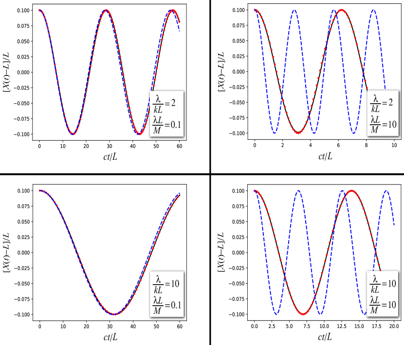
Figure 3: Time dependence of the displacement (with respect to the equilibrium position $X=L$) of the mass $M$ attached to the end of the spring, for an initial condition which, in the nonrelativistic massive regime, leads to the harmonic oscillation given by Eq. (76) with $n=1$ and $A/L=0.1$. The relativistic solution is given by the solid (black) curve, while the (red) dots represent the nonrelativistic massive case. For comparison, the (blue) dashed curve gives the position of the relativistic particle in the harmonic potential.

In Fig. 3, we plot the time dependence of the displacement (with respect to the equilibrium position $X=L$) of the mass $M$ attached to the end of the spring, for initial conditions which, in the nonrelativistic massive regime, lead to the harmonic oscillation given by Eq. (76) with $n=1$ and $A/L=0.1$. Both relativistic and nonrelativistic evolutions are plotted, as well as the position of the relativistic particle in the harmonic potential for the corresponding parameter $kL^{2}/M$ (and same initial conditions for its displacement from the equilibrium position). We see that, for $m/M\ll 1$, the three systems evolve very similarly. However, for $m/M\gg 1$, while both relativistic and nonrelativistic spring-mass evolutions continue to be very similar (for this choice of parameters and initial conditions), they differ significantly from the harmonic-potential one. This can be qualitatively understood considering that the potential energy initially available is converted not only to kinectic energy of the mass $M$ but also of the spring elements. Therefore, $M$ moves slower when attached to the massive spring than it would in the harmonic potential (with similar initial potential energy) — and this effect is more important the larger the value of $m/M$.

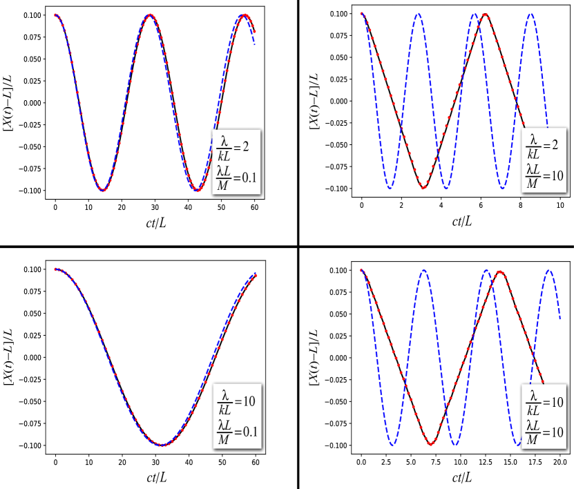
Figure 4: Time dependence of the displacement (with respect to the equilibrium position $X=L$) of the mass $M$ attached to the end of the spring, for a spring which is initially homogeneously stretched (by 10%) and at rest. As in the previous figure, the relativistic solution is given by the solid (black) curve, while the (red) dots represent the nonrelativistic massive case. For comparison, the (blue) dashed curve gives the position of the relativistic particle in the harmonic potential.

In Fig. 4, we plot the very same quantities as in Fig. 3, only changing initial conditions to be those of a spring homogeneoulsy stretched (by 10% of its natural length), at rest. We see that the previous discussion applies equally well to this case, with the additional point that for non-negligible $m/M$, the motion of the mass $M$ attached to the spring is no longer harmonic. This is expected on the grounds that a massive spring has an infinite number of oscillation modes and the homogeneously stretched spring excites all of them (see discussion in Appendix B). Nonetheless, the nonrelativistic massive-spring evolution continues to approximate very well the relativistic system. Finally, in Fig. 5 we plot the same quantities as in the previous figures — with initial conditions analogous to Fig. 3 —, but now choosing the parameters in such a way that one can perceive a (small) difference between the evolutions of the relativistic spring-mass system and the nonrelativistic one. Notwithstanding, even in this ultra-relativistic regime, the relativistic spring-mass system is farly approximated by the nonrelativistic one. Attempts to find ultra-relativistic regimes where this approximation would fail led to numerical solutions which develop shock waves (signaled by $s\leq 0$), for which our spring model would not be physically plausible.

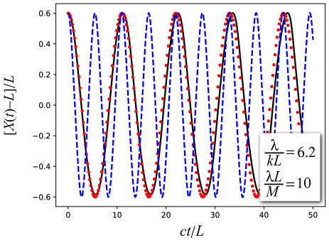
Figure 5: Same as Fig. 3 (with same style code), but now for a particular choice of parameters which lead to an ultra-relativistic regime, where a difference between the relativistic and the nonrelativistic massive spring can be perceived.

VIII Discussions

We have presented a comprehensive treatment of the relativistic one-dimensional Hookean spring-mass system in Minkowski spacetime. In order to comply with causality, the spring mass $m$ must be explicitly taken into account. Interestingly enough, causality is guaranteed if, and only if, the weak energy condition (which is equivalent to the strong energy condition in this case) is verified. In order to see how relativistic contributions impact on the spring-mass system, we first analyze the nonrelativistic regime for massive springs and verified that up to order $m/M$, the motion of the mass $M$ attached at the spring tip will oscillate harmonically with frequency $\omega_{0}[1-m/(6M)]$ up to some time interval of order $(M/m)\omega_{0}^{-1}$, $\omega_{0}=\sqrt{k/M}$. Next, we have investigated how the nonrelativistic dynamics is impacted by first-order relativistic corrections in $\vartheta/c$. It is interesting to notice that the relativistic dynamics was found to be important not only in the regime of high velocities (compared to $c$) but also in the regime of high tensions (which may appear in super-hard springs). This can be seen from the fact that both $u\ll c$ (small matter velocities) and $\vartheta\ll c$ (small sound speed) must be assumed in order to obtain the nonrelativistic equation of motion (51) from the relativistic one, Eq. (28). Finally, we have performed numerical calculations which attest that the full relativistic spring-mass system is much better approximated by the nonrelativistic massive case than by the so-called relativistic harmonic oscillator (1). Total energy conservation is guaranteed by Eq. (50) and can be used (as it was, in the numerical calculations) to monitor the system evolution.

Appendix A

Let us assume a charge $q$ with mass $M$ under the influence of a fixed external electromagnetic field. The corresponding equation of motion will be given by

$$F^{b}=Ma^{b}$$ (110)

with the Lorentz force (in CGS units):

$$F^{b}=(q/c){\cal F}^{bc}u_{c},$$ (111)

where $u^{b}$ and $a^{b}$ are the charge 4-velocity and 4-acceleration, respectively. Now, let us assume that the following Faraday tensor approximates the electromagnetic field in some region:

$${\cal F}^{ab}=(k/q)(x_{c}X^{c})(X^{a}V^{b}-V^{a}X^{b}),$$ (112)

where $k$ is a positive constant, $x^{a}$ locates spacetime points with respect to some (arbitrarily chosen) spacetime “origin,” $V^{a}$ is a constant timelike, unit vector field (i.e., $V_{a}V^{a}=1$, $\nabla_{a}V^{b}=0$) which can be associated with the 4-velocity of a congruence of inertial Killing observers, while $X^{a}$ is a constant spacelike, unit vector field orthogonal to $V^{a}$ (i.e., $X_{a}X^{a}=-1$, $\nabla_{a}X^{b}=0$, and $X^{a}V_{a}=0$). Under this assumption, the force (111) acquires the form

$$F^{a}\equiv(k/c)(x_{c}X^{c})(X^{a}\;V^{b}-V^{a}\;X^{b})u_{b},$$ (113)

which leads to Eqs. (1) and (2), with Hooke’s potential $\Phi=k(x^{a}X_{a})^{2}/2$, when substituted into Eq. (110) and, then, projected along $X^{a}$ and $V^{a}$, respectively. It rests to understand to which electric and magnetic fields Eq. (112) corresponds. According to observers of the inertial congruence, this corresponds to the electric field

$$E_{X}=F^{ab}V_{a}X_{b}=-(k/q)|x^{a}X_{a}|$$ (114)

and to no magnetic field. One can easily see that such an electric field is found in the interior of a thick plate having constant charge density $\rho=-k/(4\pi q)$ and surface linear dimensions much larger than its width. In this case, the electric field (114) is perpendicular to the plate’s surface. Thus, a charge $q>0$ with mass $M$ moving inside such a plate perpendicularly to its surface will oscillate as described by Eqs. (1) and (2), with $(t,x,y,z)$ being the Cartesian coordinates attached to the (preferred) laboratory reference frame where the plate lies at rest. Causality is not an issue here because the external potential is fixed a priori, in contrast to the spring-mass system where the corresponding potential depends on the spring state at each moment.

Appendix B

Here, we will determine the dynamics of a (nonrelativistic) massive spring with one end fixed to a inertial wall and the other one attached to a massive body with mass $M\gg m$, where we recall that $m=\lambda L$ is the spring’s mass. To this end, it will be convenient to define the new function $\tilde{x}(t,l)=x(t,l)-l$ in order to make the system of equations being solved homogeneous. It is easy to see from Eqs. (51), (53), and (54) that $\tilde{x}$ satisfy the nonrelativistic spring equation

$$\frac{1}{\vartheta^{2}}\frac{\partial^{2}\tilde{x}}{\partial t^{2}}-\frac{\partial^{2}\tilde{x}}{\partial l^{2}}=0$$ (115)

as well as the boundary conditions $\tilde{x}(t,0)=0$ and

$$\left.\left(\frac{\partial^{2}\tilde{x}}{\partial t^{2}}+\omega_{0}^{2}L\frac{\partial\tilde{x}}{\partial l}\right)\right|_{(t,L)}=0$$ (116)

at $l=0$ and $l=L$, respectively. We note that the boundary condition at $l=L$ is now given by a homogeneous equation, in contrast with Eq. (54). Next, we write the function $\tilde{x}$ as the product of two independent functions

$$\tilde{x}(t,l)=\tau(t)\Lambda(l)$$ (117)

and insert this into Eq. (115) to get

$$\frac{d^{2}\Lambda}{dl^{2}}+\chi^{2}\Lambda=0$$ (118)

and

$$\frac{d^{2}\tau}{dt^{2}}+\chi^{2}\vartheta^{2}\tau=0,$$ (119)

where $\chi$ is some real constant. Due to the boundary conditions, we will need to consider only the case $\chi\neq 0$ since when $\chi=0$ the corresponding solution for $\tilde{x}$ vanishes. As a result, the general solutions of Eqs. (118) and (119) are given by

$$\Lambda(l)=\sin{(\chi l)}$$ (120)

and

$$\tau(t)=a\sin{(\chi\vartheta t)}+b\cos{(\chi\vartheta t)},$$ (121)

respectively, where we have already imposed the boundary condition $\tilde{x}(t,0)=0$ at $l=0.$ To impose the boundary condition at $l=L,$ we first use the spring equation (115) to rewrite Eq. (116) as

$${\left.\left(\frac{\partial^{2}\tilde{x}}{\partial l^{2}}+\frac{\omega_{0}^{2}L}{\vartheta^{2}}\frac{\partial\tilde{x}}{\partial l}\right)\right|}_{(t,L)}=0.$$ (122)

By plugging Eq. (117) in the above equation we find that $\Lambda$ satisfies

$$\left.\left(\frac{d^{2}\Lambda}{dl^{2}}+\frac{\omega_{0}^{2}L}{\vartheta^{2}}\frac{d\Lambda}{dl}\right)\right|_{l=L}=0$$ (123)

which, together with Eq. (120), gives the relation

$$\chi L=\frac{m}{M}\cot{(\chi L)}.$$ (124)

This is a transcendental equation for $\chi$ and its solutions, $\chi_{n}$, can be labeled by nonzero integer index $n$ arranged such that

$$\ldots<\chi_{-2}<\chi_{-1}<0<\chi_{1}<\chi_{2}<\ldots$$

and $\chi_{-n}=-\chi_{n}$. Hence, we can retain only the solutions with $n>0$ inasmuch as they are completely equivalent to the ones with $n<0.$ As a result, the general solution for the massive spring equation satisfying our boundary conditions is

$$x(t,l)=l+\sum_{n=1}^{\infty}\left[a_{n}\sin{\left(\chi_{n}\vartheta t\right)}+b_{n}\cos{\left(\chi_{n}\vartheta t\right)}\right]\sin{\left(\chi_{n}l\right)}.$$ (125)

Now, the initial conditions (38) and (39) may be used to determine the coefficients $a_{n}$ and $b_{n}$ since

$$q(l)=l+\sum_{n=1}^{\infty}b_{n}\sin{\left(\chi_{n}l\right)}$$ (126)

and

$$v(l)=\vartheta\sum_{n=1}^{\infty}a_{n}\chi_{n}\sin{\left(\chi_{n}l\right)}.$$ (127)

The problem is that these are expansions in terms of functions that are not orthogonal, making it difficult to explicitly solve for the coefficients. Nonetheless, the situation is considerably simplified in the light spring case. From Eq. (124) we can see that, when $m/M\ll 1$, $\chi_{1}L\ll 1$ and $\chi_{n+1}L\approx n\pi$. Hence, to lowest order, i.e., $\tan{\chi_{1}L}\approx\chi_{1}L$, we find that $\chi_{1}L\approx\sqrt{m/M}$ and thus

$$q(l)=l+b_{1}\sqrt{\frac{m}{M}}\frac{l}{L}+\sum_{n=1}^{\infty}b_{n+1}\sin{\left(n\pi\frac{l}{L}\right)}$$ (128)

and

$$v(l)=\frac{\vartheta}{L}\left[a_{1}\frac{m}{M}\frac{l}{L}+\sum_{n=1}^{\infty}n\pi a_{n+1}\sin{\left(n\pi\frac{l}{L}\right)}\right].$$ (129)

The coefficient $a_{1}$ and $b_{1}$ can be easily determined by evaluating the above equations at $l=L$, yielding

$$a_{1}=\frac{ML}{m\vartheta}v(L)$$ (130)

and

$$b_{1}=\sqrt{\frac{M}{m}}(q(L)-L),$$ (131)

respectively. To determine the coefficients $a_{n}$ and $b_{n}$ for $n>1$, we just use the orthogonality of the basis functions, $\sin{\left(n\pi\frac{l}{L}\right)},$ to obtain

$$a_{n+1}=\frac{2}{n\pi\vartheta}\int_{0}^{L}dl\left[v(l)-v(L)\frac{l}{L}\right]\sin{\left(n\pi\frac{l}{L}\right)}$$ (132)

and

$$b_{n+1}=\frac{2}{L}\int_{0}^{L}dl\left[q(l)-q(L)\frac{l}{L}\right]\sin{\left(n\pi\frac{l}{L}\right)}.$$ (133)

As a result, the solution describing a very light spring is

$$x(t,l)=l+\sqrt{\frac{m}{M}}\left[a_{1}\sin{(\omega_{0}t)}+b_{1}\cos{(\omega_{0}t)}\right]\frac{l}{L}$$

$$+\sum_{n=1}^{\infty}\sin{\left(n\pi\frac{l}{L}\right)}\left[a_{n+1}\sin{\left(\omega_{n}t\right)}\ +b_{n+1}\cos{\left(\omega_{n}t\right)}\right],$$

where $\omega_{n}\equiv n\pi\sqrt{M/m}\,\omega_{0}$. and we can see the terms coming from the massless spring’s equation in the first line, which we call slow waves, and in the second line the series representing what we call fast waves. These fast waves are responsible to enable arbitrary freedom in the choice of initial conditions. We note, however, that in this lowest order approximation the motion of the body is not affected by these fast waves since $X(t)=x(t,L)$ is given by

$$X(t)=L+\left[a^{\prime}_{1}\sin{(\omega_{0}t)}+b^{\prime}_{1}\cos{(\omega_{0}t)}\right],$$ (135)

where $a^{\prime}_{1}=\sqrt{m/M}a_{1}$ and $b^{\prime}_{1}=\sqrt{m/M}b_{1},$ which we recognize to be the massless spring solution (66). Notwithstanding this, the above procedure will be useful when calculating the first correction to the motion of the body coming from the spring mass.

To determine such correction, let us write

$$x(t,l)=x_{0}(t,l)+\epsilon(t,l)$$ (136)

where $\epsilon(t,l)$ is a perturbation of order $m/M$ over the spring solution $x_{0}(t,l)$ given by the right-hand side of Eq. (B). It should be stressed that even though $\epsilon$ is assumed to be a perturbation of small amplitude, it will enter the equations with the same importance as the unperturbed solution due to the fast waves, which have a substantial second derivative in time.

For the sake of simplicity, we will consider the case where the spring is held stretched for a while and then released from rest, in which case

$$q(l)=l\left(1+\frac{A}{L}\right)$$ (137)

and

$$v(l)=0.$$ (138)

By using the above initial conditions in Eqs. (130)-(B), the unperturbed solution can be written as

$$x_{0}(t,l)=l\left(1+\frac{A}{L}\cos{(\omega_{0}t)}\right).$$ (139)

If we now use Eqs. (136) and (139) in Eq. (51), we find that $\epsilon$ satisfies the inhomogeneous equation

$$\frac{1}{\vartheta^{2}}\frac{\partial^{2}\epsilon}{\partial t^{2}}-\frac{\partial^{2}\epsilon}{\partial l^{2}}=\frac{m}{M}\frac{Al}{L^{3}}\cos{(\omega_{0}t)}.$$ (140)

The boundary conditions and initial conditions for $\epsilon$ are straightforward obtained from Eqs. (53), (54), and (136) yielding

$$\epsilon(t,0)=0,\;\;\;\;\left.\left(\frac{\partial^{2}\epsilon}{\partial t^{2}}+\omega_{0}^{2}L\frac{\partial\epsilon}{\partial l}\right)\right|_{(t,L)}=0$$ (141)

for the boundary conditions and

$$\epsilon(0,l)=0,\;\;\;\left.\frac{\partial\epsilon}{\partial t}\right|_{(0,l)}=0$$ (142)

for the initial conditions.

To solve the above equations, it is convenient to separate $\epsilon$ in two parts:

$$\epsilon(t,l)=\alpha(t,l)+\beta(t,l),$$ (143)

such that $\alpha$ is a slow-varying solution solving the inhomogeneous equation (140), while $\beta$ will include slow- and fast-varying solutions solving the homogeneous wave equation

$$\frac{1}{\vartheta^{2}}\frac{\partial^{2}\beta}{\partial t^{2}}-\frac{\partial^{2}\beta}{\partial l^{2}}=0.$$ (144)

As we have some freedom in choosing the initial and boundary conditions for $\alpha$ and $\beta$, let us impose $\alpha(t,0)=0$ and

$$\left.\left(\frac{\partial^{2}\alpha}{\partial t^{2}}+\omega_{0}^{2}L\frac{\partial\alpha}{\partial l}\right)\right|_{(t,L)}=0.$$ (145)

(Eventually, we confirm that the solution $\alpha(t,l)$ obtained in this way is in agreement with our previous assumption that $\alpha(t,l)$ is slow varying.) This implies that $\beta$ satisfies

$$\beta(t,0)=\epsilon(t,0)-\alpha(t,0)=0$$ (146)

$$\left.\left(\frac{\partial^{2}\beta}{\partial t^{2}}+\omega_{0}^{2}L\frac{\partial\beta}{\partial l}\right)\right|_{(t,L)}=0.$$ (147)

Since $\alpha$ is a slow-varying function, let us try the following solution

$$\alpha(t,l)=-\frac{A}{6}\frac{m}{M}\frac{l^{3}}{L^{3}}\cos{(\omega_{0}t)}+a(t)l+b(t)$$ (148)

for the equation

$$\frac{1}{\vartheta^{2}}\frac{\partial^{2}\alpha}{\partial t^{2}}-\frac{\partial^{2}\alpha}{\partial l^{2}}=\frac{m}{M}\frac{Al}{L^{3}}\cos{(\omega_{0}t)},$$ (149)

where $a(t)$ and $b(t)$ are arbitrary smooth functions. By imposing the boundary conditions at $l=0$ and $l=L$ we find that $b(t)=0$ and $a(t)$ satisfies

$$\frac{d^{2}a}{dt^{2}}+\omega_{0}^{2}a=\frac{A}{3L}\frac{m}{M}\omega_{0}^{2}\cos{(\omega_{0}t)}.$$ (150)

We will take $a(t)$ to be the following particular solution of the above equation:

$$a(t)=\frac{A}{6L}\frac{m}{M}\omega_{0}t\sin{(\omega_{0}t)},$$ (151)

which enable us to cast a particular solution of $\alpha$ as

$$\alpha(t,l)=-\frac{Al^{3}}{6L^{3}}\frac{m}{M}\cos{(\omega_{0}t)}+\frac{Al}{6L}\frac{m}{M}\omega_{0}t\sin{(\omega_{0}t)}.$$ (152)

Now, we demand

$$\omega_{0}t\ll\frac{M}{m}$$ (153)

to guarantee that Eq. (152) approximates a solution of Eq. (149). As a result, our perturbed solution is expected to be accurate only up to a certain time interval. However, since $M/m\gg 1$, many cycles of oscillation will take place during this time interval.

Now, we note from Eqs. (144)-(147) that the problem of finding the solution for $\beta$ is exactly the same problem we have already solved for the light spring case [see Eqs. (115)-(116)] with initial conditions

$$\beta(0,l)=\epsilon(0,l)-\alpha(0,l)=\frac{A}{6}\frac{m}{M}\frac{l^{3}}{L^{3}}\omega_{0}^{2}$$ (154)

and

$$\frac{\partial\beta}{\partial t}(0,l)=\frac{\partial\epsilon}{\partial t}(0,l)-\frac{\partial\alpha}{\partial t}(0,l)=0.$$ (155)

Hence, we can use Eq. (B) together with Eqs. (130)-(133) to find that $\beta$ is given by

$$\beta(t,l)=A\frac{m}{M}\left[\frac{l}{6L}\cos{(\omega_{0}t)}\right.$$

$$+\left.\frac{2}{\pi^{3}}\sum_{n=1}^{\infty}\frac{(-1)^{n}}{n^{3}}\sin{\left(n\pi\frac{l}{L}\right)}\cos{\left(\omega_{n}t\right)}\right].$$ (156)

As a result, using Eqs. (139), (143), (152), and (B) in Eq. (136), we find that the solution for the spring equation corrected to first order in $m/M$ and satisfying the boundary conditions (53)-(54) as well as initial conditions (137)-(138) is

$$x(t,l)=l\left(1+\frac{A}{L}\cos{(\omega_{0}t)}\right)$$

$$+ \frac{A}{6}\frac{m}{M}\frac{l}{L}\left[\left(1-\frac{l^{2}}{L^{2}}\right)\cos{\left(\omega_{0}t\right)}+\omega_{0}t\sin{(\omega_{0}t)}\right]$$

$$+ A\frac{m}{M}\frac{2}{\pi^{3}}\sum_{n=1}^{\infty}\frac{(-1)^{n}}{n^{3}}\sin{\left(n\pi\frac{l}{L}\right)}\cos{\left(\omega_{n}t\right)}.$$

References

- (1) R. Penfield and H. Zatkis, The relativistic linear harmonic oscillator, J. Franklin Institute 262, 121 (1956).
- (2) E. H. Hutten, Relativistic (non-linear) oscillator, Nature 205, 535 (1965).
- (3) J. H. Kim, S. W. Lee, H. Maassen, and H. W. Lee, Relativistic oscillator of constant period, Phys. Rev. A 53, 2991 (1996).
- (4) H. Goldstein, C. P. Poole, and J. L. Safko, Classical Mechanics, 3rd ed. (Addison-Wesley, San Francisco, 2000), p.316.
- (5) R. Beig and B. G. Schmidt, Relativistic elasticity, Class. Quantum Grav. 20, 889 (2003).
- (6) R. Beig and M. Wernig-Pichler, On the motion of a compact elastic body, Commun. Math. Phys. 271, 455 (2007).
- (7) We note that nonlongitudinal pressures and shear stresses, if any, should not affect our results because of the one-dimensional feature of our problem.
- (8) On physical grounds, must be a monotonically increasing function of , while .
- (9) The missing of all but one solution unveils the non-perturbative character of the light spring case over the massless spring one. This is actually reasonable as perturbations travel extremely fast on a very light spring. This can be easily seen by noting that the massless spring equation cannot deal with situations where the spring is released from an inhomogeneous configurations. The massive spring equation, however, will be able to handle this by superposing to the slowly oscillating modes some very fast oscillating ones.
- (10) The higher modes exhibit maximum velocities of similar order, if one assumes small deformations.
- (11) We note that this boundary condition demands for , but it says nothing about the relation between and for . We can, however, extend the validity of the condition to the whole domain provided that it is still possible to satisfy the boundary condition at and allow arbitrary initial conditions.