Winding of a Brownian particle
around a point vortex

Abstract

We derive the asymptotic winding law for a Brownian particle in the plane subjected to a tangential drift due to a point vortex. For winding around a point, the normalized winding angle converges to an inverse Gamma distribution. For winding around a disk, the angle converges to a distribution given by an elliptic theta function. For winding in an annulus, the winding angle is asymptotically Gaussian with a linear drift term. We validate our results with numerical simulations.

1 Introduction

Let $\bm{R}(t)$ be a two-dimensional Brownian motion in $\mathbb{R}^{2}$ with unit diffusivity, so that $\mathbb{E}|\bm{R}(t)|^{2}=4t$. Take $\Theta(t)$ to be the total winding angle with respect to the origin accumulated by $\bm{R}(t)$ up to time $t$. It is a known fact that Brownian motion avoids the origin with probability $1$, so the winding angle is well-defined. Since the winding angle takes value in $(-\infty,\infty)$ instead of $[0,2\pi)$, we can view the Brownian motion as taking place in the universal cover of $\mathbb{C}\backslash\{0\}$, i.e., the Riemann surface of $\log z$.

Spitzer [14] in 1958 showed that the normalized winding angle converges to a standard Cauchy distribution as $t\rightarrow\infty$,

(1) $$\frac{2\Theta(t)}{\log t}\xrightarrow{\enskip d\enskip}X,\qquad p_{X}(x)=\frac{1}{\pi}\frac{1}{1+x^{2}}\,,$$

where $p_{X}(x)$ denotes the probability density of $X$. Spitzer proved this by solving the Kolmogorov backward equation in a wedge region, then taking the limit of infinite wedge angle. A key feature of Spitzer’s law is that the winding angle has infinite variance, which is due to the roughness of the Brownian trajectory generating large winding near the origin [13]. In fact, all positive integer moments diverge. This divergence is undesirable when modeling physical problems, such as flexible polymers, and there are several ways to regularize it.

Instead of a continuous process such as Brownian motion, let $\bm{R}(n)$ be a random walk on a square lattice of $\mathbb{R}^{2}$ that avoids the origin, with i.i.d. steps $\Delta\bm{R}$. Bélisle [1] showed that if $\Delta\bm{R}$ is bounded or absolutely continuous with respect to Lebesgue measure, then the winding angle follows a standard hyperbolic secant distribution,

(2) $$\frac{2\Theta(n)}{\log n}\xrightarrow{\enskip d\enskip}X,\qquad p_{X}(x)=\tfrac{1}{2}\operatorname{sech}(\pi x/2),$$

as $n\rightarrow\infty$. All moments now exist, since it is impossible for $\bm{R}(n)$ to get infinitely close to the origin to generate large winding. The main idea behind the proof, introduced by Messulam & Yor [12], is to consider two types of windings, the big windings (accumulated outside of a certain disk) and the small windings (accumulated inside). The same result was obtained by Rudnick & Hu [13] using a different method. Berger [3] and Berger & Roberts [4] studied a walk with random angle but fixed step length and also observed convergence to Eq. 2.

Another way to regularize the original problem is to put a finite-sized obstacle around the origin to prevent $\bm{R}(t)$ from entering its vicinity. Specifically, let $\bm{R}(t)$ be a planar Brownian motion as above but with a disk of radius $a$ carved out around the origin. Assuming reflecting boundary conditions on the disk’s boundary, Grosberg & Frisch [8] showed that

(3) $$\frac{2\Theta(t)}{\log(4t/a^{2})}\xrightarrow{\enskip d\enskip}X,\qquad p_{X}(x)=\tfrac{1}{2}\operatorname{sech}(\pi x/2).$$

Revisiting Spitzer’s case, they also gave a more precise normalization factor for the winding angle, but we shall see in Appendix C that a small correction is needed.

In the present paper we derive asymptotic winding laws for a Brownian particle subjected to a point vortex at the origin. The drift due to the point vortex is in the tangential direction in the standard polar coordinates, and its amplitude has magnitude $\beta/r^{2}$, where $\beta>0$ and $r$ is the distance from the origin. This kind of vortical drift arises in inviscid fluid motion [10]. Moreover, we shall see that this particular tangential drift preserves eigensolutions of the separated Fokker–Planck equation in the form of Bessel functions, albeit with complex argument, and is thus amenable to analytical treatment. We find the limit distribution for three natural cases:

(i)

For the case where the particle winds around the origin (Figs. 1a and 3), we find convergence to an inverse Gamma distribution, i.e.,

(4) $$\frac{\beta\log^{2}\!{\left(4t/r_{0}^{2}\,{\mathrm{e}}^{\gamma}\right)}}{8\Theta(t)}\xrightarrow{\enskip d\enskip}\operatorname{Gamma}(\tfrac{1}{2},\tfrac{1}{2}),$$

where $r_{0}$ is the initial radial coordinate, and $\gamma$ is the Euler–Mascheroni constant.

(ii)

When the particle winds outside a disk of radius $a$ (Figs. 1b and 4), the winding angle distribution converges to the derivative $\vartheta_{2}^{\prime}$ of a second elliptic theta function,

(5) $$\frac{4\Theta(t)}{\beta\,\log^{2}({4t}/{a^{2}\,{\mathrm{e}}^{2\gamma}})}\xrightarrow{\enskip d\enskip}X,\qquad p_{X}(x)=-\tfrac{\pi}{2}\,\vartheta_{2}^{\prime}\bigl{(}\tfrac{\pi}{2}\,,\,{\mathrm{e}}^{-\pi^{2}x}\bigr{)}\,\chi_{(x>0)}\,,$$

where by convention the derivative in $\vartheta_{2}^{\prime}$ is with respect to the first argument, and $\chi$ is the indicator function.

(iii)

Finally, we show that for a particle winding inside an annulus $a<r<b$ (Figs. 1c and 5), the winding angle distribution converges to a Gaussian with linear drift:

(6) $$\frac{\Theta(t)-A(t)\beta}{\sqrt{2A(t)}}\xrightarrow{\enskip d\enskip}N(0,1),\qquad A(t)=\frac{2t}{b^{2}-a^{2}}\log(b/a).$$

In all three cases we compare to numerical simulations to exhibit the convergence to the limiting distribution. Because the normalizers in the first two cases are logarithmic in $t$, it is crucial to have the precise $\mathcal{O}\!\left(1\right)$ constants inside the $\log$ when comparing to numerical results, since otherwise astronomical values of $t$ are required to see convergence.

Existing results most closely related to ours either involve drift or bias the Brownian motion in some way to promote winding. Le Gall & Yor [11] analyze a general planar Brownian motion with drift and obtain a modification of Spitzer’s law. However, their drift must satisfy an integrability condition that fails for a point vortex. Comtet et al. [5] studied diffusion with drift $-\nabla\mathcal{U}(r)$ due to a radial potential in a disk of radius $R$. By picking the special form $\mathcal{U}=(\alpha-1)\log(-\log(r/R_{0}))$, they found an $\alpha$-stable Lévy distribution for the normalized winding angle $X(t)=\Theta(t)/t^{1/\alpha}$, with $1\leq\alpha^{2}<4$. They found convergence to a Gaussian winding angle for an annular domain. Toby & Werner [15] showed that Brownian motion reflected at an angle along an outer boundary also increases the winding. Drossel & Kardar [6] observed that chiral defects can promote winding. Vakeroudis [16] considered winding of a complex Ornstein–Uhlenbeck process.

2 Brownian motion with tangential drift

Consider the two-dimensional continuous-time stochastic process $\bm{R}(t)=(R_{1}(t),R_{2}(t))$, starting at a point $\bm{R}(0)=\bm{r}_{0}\neq\bm{0}$, and obeying the SDE

(7) $$\mathop{}\!\mathrm{d}\bm{R}=\bm{R}^{\perp}\,\Omega(\lvert\bm{R}\rvert,t)\mathop{}\!\mathrm{d}t+\sqrt{2}\,\mathop{}\!\mathrm{d}\bm{W}$$

where $\bm{R}^{\perp}=(-R_{2},R_{1})$ and $\bm{W}(t)$ is a vector of two independent standard Brownian motions. The function $\Omega(r,t)$ corresponds to a tangential drift that spins particles around the origin.

Let $p(\bm{r},t\,|\,\bm{r}_{0},0)$ be the transition probability density of $\bm{R}(t)$, which satisfies the Fokker–Planck equation

(8) $$\frac{\partial p}{\partial t}+\Omega(r,t)\,\frac{\partial p}{\partial\theta}=\Delta p,\qquad p(\bm{r},0\,|\,\bm{r}_{0},0)=\delta(\bm{r}-\bm{r}_{0}).$$

Our main goal is to study the case where $\Omega(r,t)=\beta/r^{2}$, for a constant $\beta>0$, which corresponds to the flow field around a steady two-dimensional point vortex [10]. Without loss of generality, we take $\bm{r}_{0}=(r_{0},0)$ with $r_{0}>0$. Define in polar coordinates

(9) $$P(r,\theta,t)=p(\bm{r},t\,|\,\bm{r}_{0},0)$$

where we suppressed the $r_{0}$ dependence for simplicity. Equation 8 is now

(10) $$\frac{\partial P}{\partial t}+\frac{\beta}{r^{2}}\frac{\partial P}{\partial\theta}=\frac{\partial P}{\partial r}+\frac{1}{r}\frac{\partial P}{\partial r}+\frac{1}{r^{2}}\frac{\partial P}{\partial\theta},\qquad P(r,\theta,0)=\frac{1}{r}\,\delta(r-r_{0})\,\delta(\theta).$$

Equation 10 has separated solutions of the form

(11) $${\mathrm{e}}^{-\lambda^{2}t}\,{\mathrm{e}}^{\mathrm{i}\mu\theta}\,\rho(r)$$

where $0<\lambda\in\mathbb{R}$, $\mu\in\mathbb{R}$, and $\rho(r)$ obeys the eigenvalue problem

(12) $$\rho^{\prime\prime}+\frac{1}{r}\rho^{\prime}+\biggl{(}\lambda^{2}-\frac{k_{\mu}^{2}}{r^{2}}\biggr{)}\rho=0,\qquad k_{\mu}=\sqrt{\mu^{2}+\mathrm{i}\beta\mu}\,,$$

where we take the branch for $k_{\mu}$ with nonnegative real part. Normally, Eq. 10 is solved with $2\pi$-periodic boundary conditions in $\theta$, so that $\mu$ is a discrete eigenvalue. However, to take the winding into account we must allow for $-\infty<\theta<\infty$, with the boundary conditions that $P(r,\pm\infty,t)=0$. From here, the solution to Eq. 12 depends on boundary conditions in $r$, which naturally divide our discussion into three cases: winding around a point (Section 3), around a disk (Section 4), and inside an annulus (Section 5).

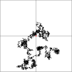
(a)

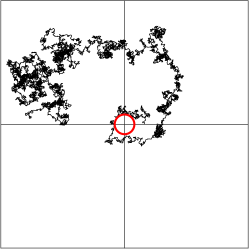
(b)

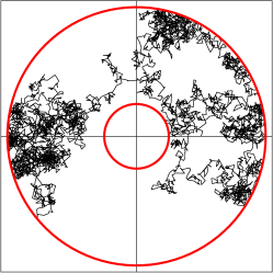
(c)

Figure 1: (a) Winding of a Brownian particle around the origin, starting from $\bm{R}(0)=(1,0)$, subjected to a central point vortex of strength $\beta=1$. (b) Winding around a disk of radius $a=1/2$ with $\beta=3$; (c) Winding in an annulus with inner radius $a=1/2$, outer radius $b=2$, with $\beta=1$. Note the tendency of the path to wind counterclockwise because of the influence of the point vortex.

3 Winding around a point

For winding around the origin, the domain of Eq. 12 is $0<r<\infty$. As a result, only Bessel functions of the first kind are involved, so the solution to Eq. 8 is

(13) $$P(r,\theta,t)=\frac{1}{2\pi}\int_{-\infty}^{\infty}\int_{0}^{\infty}{\mathrm{e}}^{-\lambda^{2}t}{\mathrm{e}}^{\mathrm{i}\mu\theta}J_{k_{\mu}}(\lambda r)\,J_{k_{\mu}}(\lambda r_{0})\,\lambda\mathop{}\!\mathrm{d}\lambda\mathop{}\!\mathrm{d}\mu\,,$$

where $k_{\mu}$ is defined in Eq. 12, and $J_{\nu}$ is a Bessel functions of the first kind of order $\nu$. Since we are interested in the asymptotic behavior of $P(r,\theta,t)$ as $t\rightarrow\infty$, the $\lambda$ integral is dominated by small $\lambda$ (Watson’s Lemma [2]). Therefore, we can choose $t$ large enough such that

(14) $$J_{k_{\mu}}(\lambda r_{0})\sim\frac{1}{\Gamma(1+k_{\mu})}\left(\frac{\lambda r_{0}}{2}\right)^{k_{\mu}},\qquad\lambda r_{0}\ll\sqrt{\lvert 1+k_{\mu}\rvert}.$$

The restriction $\lambda r_{0}\ll\sqrt{\lvert 1+k_{\mu}\rvert}$ means that we can use this to approximate $J_{k_{\mu}}(\lambda r_{0})$, but not necessarily $J_{k_{\mu}}(\lambda r)$, since $r$ goes to infinity in the integral. With this approximation, Eq. 13 becomes

$$P(r,\theta,t) \sim\frac{1}{2\pi}\int_{-\infty}^{\infty}\int_{0}^{\infty}{\mathrm{e}}^{-\lambda^{2}t}{\mathrm{e}}^{\mathrm{i}\mu\theta}\,\frac{1}{\Gamma(1+k_{\mu})}\left(\frac{\lambda r_{0}}{2}\right)^{k_{\mu}}\,J_{k_{\mu}}(\lambda r)\,\lambda\mathop{}\!\mathrm{d}\lambda\mathop{}\!\mathrm{d}\mu$$

$$=\frac{1}{2\pi}\int_{-\infty}^{\infty}\frac{1}{\Gamma(1+k_{\mu})}\left(\frac{r_{0}}{2}\right)^{k_{\mu}}{\mathrm{e}}^{\mathrm{i}\mu\theta}\int_{0}^{\infty}{\mathrm{e}}^{-\lambda^{2}t}\lambda^{k_{\mu}+1}J_{k_{\mu}}(\lambda r)\mathop{}\!\mathrm{d}\lambda\mathop{}\!\mathrm{d}\mu\,.$$

Then the winding angle distribution is given by

$$W(\theta,t) =\int_{0}^{\infty}P(r,\theta,t)\,r\mathop{}\!\mathrm{d}r$$

(15) $$\sim\frac{1}{2\pi}\int_{-\infty}^{\infty}\frac{1}{\Gamma(1+k_{\mu})}\left(\frac{r_{0}}{2}\right)^{k_{\mu}}{\mathrm{e}}^{\mathrm{i}\mu\theta}\int_{0}^{\infty}\int_{0}^{\infty}{\mathrm{e}}^{-\lambda^{2}t}\lambda^{k_{\mu}+1}J_{k_{\mu}}(\lambda r)\,r\mathop{}\!\mathrm{d}\lambda\mathop{}\!\mathrm{d}r\mathop{}\!\mathrm{d}\mu.$$

The $r$ integral can be carried out analytically, and we have

$$W(\theta,t) \sim\frac{1}{2\pi}\int_{-\infty}^{\infty}\frac{\Gamma(1+\tfrac{k_{\mu}}{2})}{\Gamma(1+k_{\mu})}\left(\frac{r_{0}}{2\sqrt{t}}\right)^{k_{\mu}}{\mathrm{e}}^{\mathrm{i}\mu\theta}\mathop{}\!\mathrm{d}\mu$$

(16) $$\sim\frac{1}{2\pi}\int_{-\infty}^{\infty}\left(\frac{r_{0}\,{\mathrm{e}}^{\gamma/2}}{2\sqrt{t}}\right)^{k_{\mu}}{\mathrm{e}}^{\mathrm{i}\mu\theta}\mathop{}\!\mathrm{d}\mu\,,$$

where $\gamma=0.577215\ldots$ is the Euler–Mascheroni constant. In the last step we expanded the integrand in small $k_{\mu}$, since $(r_{0}/\sqrt{t})\ll 1$.

Let $A(t)=\sqrt{\beta/8}\,\log\left(4t/r_{0}^{2}\,{\mathrm{e}}^{\gamma}\right)$; then

(17) $$W(\theta,t)\sim\frac{1}{2\pi}\int_{-\infty}^{\infty}{\mathrm{e}}^{-A(t)\sqrt{2/\beta}\,k_{\mu}+\mathrm{i}\mu\theta}\mathop{}\!\mathrm{d}\mu\,.$$

Since $A(t)\rightarrow\infty$ as $t\rightarrow\infty$, the integral is dominated by small $\mu$. Note that from Eq. 12, as $\mu\rightarrow 0$,

(18) $$k_{\mu}\sim\sqrt{\mathrm{i}\beta\mu}=\sqrt{\frac{\beta|\mu|}{2}}\left(1+\mathrm{i}\operatorname{sgn}\mu\right)$$

where $\operatorname{sgn}$ is the signum function, leading to

$$W(\theta,t) =\frac{1}{2\pi}\int_{-\infty}^{\infty}{\mathrm{e}}^{-A\sqrt{|\mu|}+\mathrm{i}(\mu\theta-\operatorname{sgn}(\mu)A\sqrt{|\mu|})}\mathop{}\!\mathrm{d}\mu$$

$$=\frac{1}{\pi}\int_{0}^{\infty}{\mathrm{e}}^{-A\sqrt{\mu}}\cos(\mu\theta-A\sqrt{\mu})\mathop{}\!\mathrm{d}\mu$$

(19) $$=\frac{1}{\sqrt{2\pi}\,A^{2}}\,x^{-3/2}\,{\mathrm{e}}^{-1/2x}\,\chi_{(x>0)},\qquad x=\theta/A^{2}\,,$$

where $\chi$ is the indicator function. We conclude that the normalized winding angle at time $t\rightarrow\infty$ converges in distribution according to

(20) $$\frac{8\Theta(t)}{\beta\log^{2}\!{\left(4t/r_{0}^{2}\,{\mathrm{e}}^{\gamma}\right)}}\xrightarrow{\enskip d\enskip}X,\qquad p_{X}(x)=\frac{1}{\sqrt{2\pi}}\,x^{-3/2}\,{\mathrm{e}}^{-1/2x}\,\chi_{(x>0)}\,.$$

Remarks

1. All positive integer moments of $W$ diverges, due to the probability of infinite winding around the point-like origin, as in Spitzer’s law Eq. 1.

2. $x^{-1}$ is Gamma-distributed:

   (21) $$\frac{\beta\log^{2}\!{\left(4t/r_{0}^{2}\,{\mathrm{e}}^{\gamma}\right)}}{8\Theta(t)}\xrightarrow{\enskip d\enskip}\operatorname{Gamma}(\tfrac{1}{2},\tfrac{1}{2}).$$

3. For $\beta=0$ the leading order term of $k_{\mu}$ is no longer $\mathcal{O}\!\left(\sqrt{\mu}\right)$, rendering Eq. 19 invalid. We need to go back to Eq. 16 and use $k_{\mu}\sim\lvert\mu\rvert$, which leads to

   $$W(\theta,t) \sim\frac{1}{\pi}\int_{0}^{\infty}{\mathrm{e}}^{-\tfrac{1}{2}\,\mu\log\left(4t/r_{0}^{2}\,{\mathrm{e}}^{\gamma}\right)}\cos(\mu\theta)\mathop{}\!\mathrm{d}\mu$$

   (22) $$=\frac{1}{\pi}\,\frac{A}{A^{2}+\theta^{2}}\,,\qquad A=\tfrac{1}{2}\,\log\left(4t/r_{0}^{2}\,{\mathrm{e}}^{\gamma}\right),$$

   which is Spitzer’s law Eq. 1 with the updated normalizer of Grosberg & Frisch [8]. Our calculation adds a correction ${\mathrm{e}}^{\gamma}$ to their normalizer. (See Appendix C.)

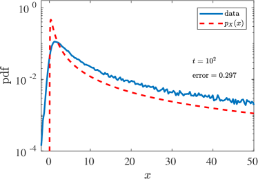
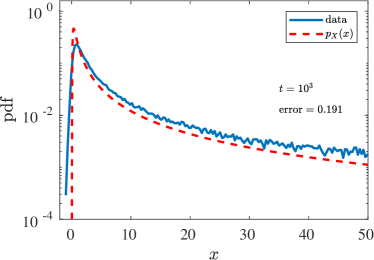
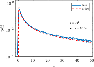
Figure 2: Numerical simulation of $10^{5}$ realizations of winding around the origin for a Brownian particle subjected to a point vortex. Here $\beta=1$ and $r_{0}=1$. The error is the $\mathrm{L}^{2}$ norm of the difference between the data and the limit distribution $p_{X}(x)$ in Eq. 20. We can see the convergence as $t\rightarrow\infty$.

4 Winding around a disk

We now remove a disk of radius $a$ centered on the origin, with reflective boundary conditions at its boundary. The particle is in the domain $a<|\bm{R}(t)|<\infty$ and so is prevented from coming close to the origin. The domain of Eq. 12 is $a<r<\infty$, with a reflecting boundary condition $\rho^{\prime}(a)=0$. The bounded solution to Eq. 12 can then be written as $\rho(r)=Z_{k_{\mu}}(\lambda r,\lambda a)$, with

(23) $$Z_{k_{\mu}}(\lambda r,\lambda a)=\frac{J_{k_{\mu}}(\lambda r)\,Y^{\prime}_{k_{\mu}}(\lambda a)-J^{\prime}_{k_{\mu}}(\lambda a)\,Y_{k_{\mu}}(\lambda r)}{\sqrt{J^{\prime 2}_{k_{\mu}}(\lambda a)+Y^{\prime 2}_{k_{\mu}}(\lambda a)}}$$

where $k_{\mu}$ is as in Eq. 12, and $J_{\nu}$, $Y_{\nu}$ are Bessel functions of the first and second kind of order $\nu$. Thus the solution to Eq. 8 is written as

(24) $$P(r,\theta,t)=\frac{1}{2\pi}\int_{-\infty}^{\infty}\int_{0}^{\infty}{\mathrm{e}}^{-\lambda^{2}t}\,{\mathrm{e}}^{\mathrm{i}\mu\theta}\,Z_{k_{\mu}}(\lambda r,\lambda a)\,Z_{k_{\mu}}(\lambda r_{0},\lambda a)\,\lambda\mathop{}\!\mathrm{d}\lambda\mathop{}\!\mathrm{d}\mu\,.$$

As in the previous Section, $t\rightarrow\infty$ allows a small-$\lambda$ approximation where we make use of the asymptotic forms

(25a) $$J_{\nu}(x) \sim\frac{(x/2)^{\nu}}{\Gamma(1+\nu)},\qquad Y_{\nu}(x) \sim\frac{(x/2)^{\nu}}{\Gamma(1+\nu)}\cot\pi\nu-\frac{(x/2)^{-\nu}}{\Gamma(1-\nu)}\csc\pi\nu,$$

(25b) $$J^{\prime}_{\nu}(x) \sim\frac{(x/2)^{\nu}\nu x^{-1}}{\Gamma(1+\nu)},\qquad Y^{\prime}_{\nu}(x) \sim\frac{(x/2)^{\nu}\nu x^{-1}}{\Gamma(1+\nu)}\cot\pi\nu+\frac{(x/2)^{-\nu}\nu x^{-1}}{\Gamma(1-\nu)}\csc\pi\nu,$$

as $x\rightarrow 0$. We thus have

(26) $$Z_{k_{\mu}}(\lambda r_{0},\lambda a)\sim\frac{(r_{0}/a)^{k_{\mu}}+(r_{0}/a)^{-k_{\mu}}}{\sqrt{[(\lambda a/2)^{k_{\mu}}\Gamma(1-k_{\mu})+(\lambda a/2)^{-k_{\mu}}\Gamma(1+k_{\mu})]^{2}-2\pi k_{\mu}\tan(\pi k_{\mu}/2)}}.$$

As we show in Appendix A, the $\mu$ integral is dominated by small $\mu$, hence small $k_{\mu}$. As $k_{\mu}\rightarrow 0$, we have $\Gamma(1-k_{\mu})\sim{\mathrm{e}}^{k_{\mu}\gamma}$, where $\gamma$ is the Euler–Mascheroni constant; $Z_{k_{\mu}}(\lambda r_{0},\lambda a)$ further simplifies

(27) $$Z_{k_{\mu}}(\lambda r_{0},\lambda a)\sim\frac{\cosh(k_{\mu}\log(r_{0}/a))}{\cosh(k_{\mu}\log(\lambda\and/2))},\qquad\and\mathrel{\raisebox{0.29707pt}{:}\!\!=}a{\mathrm{e}}^{\gamma}.$$

For $Z_{k_{\mu}}(\lambda r,\lambda a)$ in Eq. 23, as $\lambda\rightarrow 0$ we have

$$Z_{k_{\mu}}(\lambda r,\lambda a) \sim\frac{J_{k_{\mu}}(\lambda r)\left((\lambda\and/2)^{k_{\mu}}\cot{\pi k_{\mu}}+(\lambda\and/2)^{-k_{\mu}}\csc{\pi k_{\mu}}\right)-Y_{k_{\mu}}(\lambda r)(\lambda\and/2)^{k_{\mu}}}{\sqrt{\left((\lambda\and/2)^{k_{\mu}}\cot{\pi k_{\mu}}+(\lambda\and/2)^{-k_{\mu}}\csc{\pi k_{\mu}}\right)^{2}+(\lambda\and/2)^{2k_{\mu}}}}$$

(28) $$\sim J_{k_{\mu}}(\lambda r)-Y_{k_{\mu}}(\lambda r)\,\frac{(\lambda\and/2)^{k_{\mu}}\sin{\pi k_{\mu}}}{(\lambda\and/2)^{k_{\mu}}+(\lambda\and/2)^{-k_{\mu}}}.$$

The time-asymptotic winding distribution is

(29) $$W(\theta,t)\sim\frac{1}{2\pi}\int_{-\infty}^{\infty}\cosh(k_{\mu}\log(r_{0}/a))\,{\mathrm{e}}^{\mathrm{i}\mu\theta}\,\mathrm{I}_{k_{\mu}}(t)\mathop{}\!\mathrm{d}\mu$$

where

(30) $$\mathrm{I}_{k_{\mu}}(t)=\int_{a}^{\infty}\int_{0}^{\infty}{\mathrm{e}}^{-\lambda^{2}t}Z_{k_{\mu}}(\lambda r,\lambda a)\operatorname{sech}(k_{\mu}\log(\lambda\and/2))\,\lambda r\mathop{}\!\mathrm{d}\lambda\mathop{}\!\mathrm{d}r.$$

In Appendix B we show that for small $k_{\mu}$ and $t\rightarrow\infty$,

(31) $$\mathrm{I}_{k_{\mu}}(t)\sim\operatorname{sech}(k_{\mu}\log(\and/2\sqrt{t})).$$

Hence,

$$W(\theta,t) =\frac{1}{2\pi}\int_{-\infty}^{\infty}\cosh(k_{\mu}\log(r_{0}/a))\,\mathrm{I}_{k_{\mu}}(t)\,{\mathrm{e}}^{\mathrm{i}\mu\theta}\mathop{}\!\mathrm{d}\mu$$

$$\sim\frac{1}{2\pi}\int_{-\infty}^{\infty}\cosh(k_{\mu}\log(r_{0}/a))\,\operatorname{sech}(k_{\mu}\log(\and/2\sqrt{t}))\,{\mathrm{e}}^{\mathrm{i}\mu\theta}\mathop{}\!\mathrm{d}\mu$$

(32) $$=\frac{1}{2\pi A^{2}}\int_{-\infty}^{\infty}\cosh(\sqrt{\mathrm{i}\tau}B)\operatorname{sech}(\sqrt{\mathrm{i}\tau})\,{\mathrm{e}}^{\mathrm{i}\tau x}\mathop{}\!\mathrm{d}\tau$$

where

(33) $$A(t)=\tfrac{1}{2}\sqrt{\beta}\log(4t/\and^{2}),\quad B(t)=\tfrac{\sqrt{\beta}}{A(t)}\log(r_{0}/a),\quad\tau=\mu A^{2},\quad x=\theta/A^{2}.$$

The $\tau$ integral can be evaluated by computing residues at

(34) $$\tau_{n}=\mathrm{i}\pi^{2}\bigl{(}n+\tfrac{1}{2}\bigr{)}^{2},\qquad n=1,2,3,\dots.$$

We thus have

$$W(\theta,t) =\frac{2\pi\mathrm{i}}{2\pi A^{2}}\sum_{n=0}^{\infty}\pi\mathrm{i}\,(2n+1)\,(-1)^{n+1}\,{\mathrm{e}}^{-(2n+1)^{2}\pi^{2}x/4}\cos\bigl{(}\pi\bigl{(}n+\tfrac{1}{2}\bigr{)}B\bigr{)}\,\chi_{(x>0)}$$

(35) $$\sim\frac{\pi}{A^{2}}\sum_{n=0}^{\infty}(-1)^{n}\,(2n+1)\,{\mathrm{e}}^{-(2n+1)^{2}\pi^{2}x/4}\,\chi_{(x>0)},$$

where $\chi$ is the indicator function. Introduce the second elliptic theta function

(36) $$\vartheta_{2}(z,q)=2\sum_{n=0}^{\infty}q^{(2n+1)^{2}/4}\cos((2n+1)z)$$

and by convention,

(37) $$\vartheta^{\prime}_{2}(z,q)\mathrel{\raisebox{0.29707pt}{:}\!\!=}\frac{\partial\vartheta_{2}}{\partial z}(z,q).$$

Then the asymptotic winding law for the random angle $\Theta(t)$ can be expressed as

(38) $$\frac{4\Theta(t)}{\beta\,\log^{2}({4t}/{a^{2}\,{\mathrm{e}}^{2\gamma}})}\xrightarrow{\enskip d\enskip}X,\qquad p_{X}(x)=-\tfrac{\pi}{2}\,\vartheta_{2}^{\prime}\bigl{(}\tfrac{\pi}{2}\,,\,{\mathrm{e}}^{-\pi^{2}x}\bigr{)}\,\chi_{(x>0)}\,.$$

Note that now all the moments exist. The asymptotic distribution Eq. 38 is compared to numerical simulations in Fig. 3.

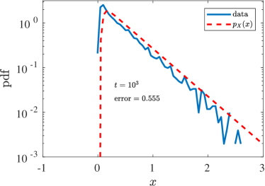
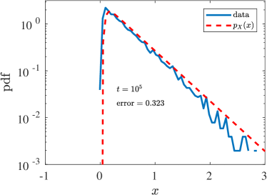
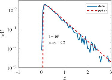
Figure 3: Numerical simulation of $10^{4}$ realizations of winding around a disk of radius $a=1/10$ for a Brownian particle subjected to a point vortex of strength $\beta=3$. The error is the $\mathrm{L}^{2}$ norm of the difference between the data and the limit distribution $p_{X}(x)$ in Eq. 38. We can see the convergence as $t\rightarrow\infty$.

5 Winding in an annulus

Finally, consider the case where the particle is confined to an annulus $a<|\bm{R}(t)|<b$, with both boundaries being reflective. Then the solution to Eq. 12 is modified accordingly to

(39) $$Z_{k_{\mu}}(\lambda r)=\frac{1}{m_{\lambda,\mu}}\left(-J_{k_{\mu}}(\lambda r)\,Y^{\prime}_{k_{\mu}}(\lambda a)+J^{\prime}_{k_{\mu}}(\lambda a)\,Y_{k_{\mu}}(\lambda r)\right)$$

where $k_{\mu}$ is as in Eq. 12, $m_{\lambda,\mu}$ is a normalization factor with

(40a) $$\int_{a}^{b}Z^{2}_{k_{\mu}}(\lambda r)\,r\mathop{}\!\mathrm{d}r=1,$$

and

(40b) $$-J^{\prime}_{k_{\mu}}(\lambda b)\,Y^{\prime}_{k_{\mu}}(\lambda a)+J^{\prime}_{k_{\mu}}(\lambda a)\,Y^{\prime}_{k_{\mu}}(\lambda b)=0,$$

in order to satisfy the reflective boundary conditions

(41) $$\frac{\partial Z_{k_{\mu}}}{\partial r}(\lambda a)=\frac{\partial Z_{k_{\mu}}}{\partial r}(\lambda b)=0.$$

The solution to Eq. 8 now involves a discrete sum over $\lambda$:

(42) $$P(r,\theta,t)=\frac{1}{2\pi}\int_{-\infty}^{\infty}\sum_{\lambda}{\mathrm{e}}^{-\lambda^{2}t}\,{\mathrm{e}}^{\mathrm{i}\mu\theta}Z_{k_{\mu}}(\lambda r)\,Z_{k_{\mu}}(\lambda r_{0})\mathop{}\!\mathrm{d}\mu.$$

The sum is over all solutions to Eq. 40b with positive real part, since we require $P(r,\theta,t)$ to stay finite as $t\rightarrow\infty$ and $Z_{\mu}(\lambda r)$ is undefined for $\lambda=0$. For fixed $\mu$, denote $\lambda_{k_{\mu}}$ the solution to Eq. 40b with smallest positive real part. For large $t$, the summation over $\lambda$ is dominated by the leading term,

(43) $${\mathrm{e}}^{-\lambda_{k_{\mu}}^{2}t}\,{\mathrm{e}}^{\mathrm{i}\mu\theta}\,Z_{k_{\mu}}(\lambda_{k_{\mu}}r)\,Z_{k_{\mu}}(\lambda_{k_{\mu}}r_{0}).$$

Using the approximations Eq. 25 for $J_{\nu}$ and $Y_{\nu}$ for small argument, we have

$$Z_{k_{\mu}}(\lambda_{k_{\mu}}r) \sim-\frac{k_{\mu}\csc\pi k_{\mu}}{m_{\lambda_{k_{\mu}},k_{\mu}}\lambda_{k_{\mu}}a\Gamma(1+k_{\mu})\Gamma(1-k_{\mu})}\left[\left(\frac{r}{a}\right)^{k_{\mu}}+\left(\frac{r}{a}\right)^{-k_{\mu}}\right]$$

$$=\frac{\cosh(k_{\mu}\log(r/a))}{C_{k_{\mu}}(a,b)}$$

where the constant $C_{k_{\mu}}(a,b)$ is determined by Eq. 40a. Hence,

(44) $$P(r,\theta,t) \sim\frac{1}{2\pi}\int_{-\infty}^{\infty}{\mathrm{e}}^{-\lambda_{k_{\mu}}^{2}t}\,{\mathrm{e}}^{\mathrm{i}\mu\theta}\,\frac{\cosh(k_{\mu}\log(r/a))\cosh(k_{\mu}\log(r_{0}/a))}{C_{k_{\mu}}^{2}(a,b)}\mathop{}\!\mathrm{d}\mu\,.$$

Before proceeding further, we prove the following:

Proposition 5.1.

As $k_{\mu}\rightarrow 0$,

1. $\lambda_{k_{\mu}}\rightarrow 0$.

2. $\displaystyle\lambda_{k_{\mu}}^{2}=\frac{2k_{\mu}^{2}}{b^{2}-a^{2}}\log(b/a)+o(k_{\mu}^{2})$.

Proof 5.2.

For the first claim, let

(45) $$\mathcal{L}=\frac{d}{dr}\left(r\frac{d}{dr}\right)-\mu^{2},\qquad\mathcal{M}=-\mathrm{i}\beta\mu\,.$$

Then Eq. 12 is rewritten as

(46) $$(\mathcal{L}+\mathcal{M})\,\rho(r)+\lambda^{2}r^{2}\rho(r)=0.$$

Consider the eigenvalue problem

(47) $$\mathcal{L}\,\phi_{\nu}(r)+\nu r^{2}\phi_{\nu}(r)=0,\quad a<r<b,\qquad\phi_{\nu}^{\prime}(a)=\phi_{\nu}^{\prime}(b)=0.$$

Sturm–Liouville theory states that the eigenvalues are real and countable, $\nu_{0}<\nu_{1}<\ldots<\nu_{n}<\ldots$, with $\lim_{n\rightarrow\infty}\nu_{n}=\infty$. By the regularity requirement of the eigenfunctions as $r\rightarrow\infty$, we have $\nu_{0}>0$. This smallest eigenvalue can be bounded by the Rayleigh quotient:

(48) $$\nu_{0}\leq-\frac{\int_{a}^{b}\phi\,\mathcal{L}\,\phi\mathop{}\!\mathrm{d}r}{\int_{a}^{b}\phi^{2}r^{2}\mathop{}\!\mathrm{d}r}=\frac{\int_{a}^{b}(r\phi^{\prime 2}(r)+\mu^{2}\phi(r))\mathop{}\!\mathrm{d}r}{\int_{a}^{b}\phi^{2}(r)r^{2}\mathop{}\!\mathrm{d}r}$$

where $\phi$ is a test function satisfying $\phi^{\prime}(a)=\phi^{\prime}(b)=0$. By choosing $\phi(r)=1$, we have

(49) $$\nu_{0}\leq\frac{3(b-a)}{b^{3}-a^{3}}\mu^{2}\rightarrow 0~{}\text{ as }\mu\rightarrow 0.$$

Since $\mathcal{L}$ and $\mathcal{M}$ commute, by [9, p. 209] the distance between the spectrum of $\mathcal{L}+\mathcal{M}$ and that of $\mathcal{L}$ is bounded by $\lVert\mathcal{M}\rVert=\beta\mu\rightarrow 0$. Hence,

(50) $$|\lambda_{k_{\mu}}^{2}-\nu_{0}|\leq\mu\rightarrow 0\quad\text{ as }\quad\mu\rightarrow 0$$

and thus $\lambda_{k_{\mu}}^{2}\rightarrow\nu_{0}\rightarrow 0$ as $\mu\rightarrow 0$, which proves the first part.

For the second part, define

(51) $$g_{k_{\mu}}(x)\mathrel{\raisebox{0.29707pt}{:}\!\!=}Y^{\prime}_{k_{\mu}}(x)/J^{\prime}_{k_{\mu}}(x)\,.$$

Then Eq. 40b is rewritten as

(52) $$g_{k_{\mu}}(\lambda a)=g_{k_{\mu}}(\lambda b)$$

and using small-$x$ asymptotics

$$g_{k_{\mu}}(x) \sim\cot(\pi k_{\mu})+\left(\frac{x}{2}\right)^{-2k_{\mu}}\frac{\Gamma(k_{\mu})\Gamma(1+k_{\mu})}{\pi}+\left(\frac{x}{2}\right)^{-2k_{\mu}+2}\frac{2(2-k_{\mu}^{2})\,\Gamma^{2}(k_{\mu})}{\pi(1-k_{\mu}^{2})}$$

$$=\cot(\pi k_{\mu})+\left(\frac{x}{2}\right)^{-2k_{\mu}}\frac{\Gamma^{2}(k_{\mu})}{\pi}\left[k_{\mu}+\left(\frac{x}{2}\right)^{2}\frac{2(2-k_{\mu}^{2})}{(1-k_{\mu}^{2})}\right].$$

So $\lambda_{k_{\mu}}$ satisfies

(53) $$a^{-2k_{\mu}}\left[k_{\mu}+\left(\frac{\lambda_{k_{\mu}}a}{2}\right)^{2}\frac{2(2-k_{\mu}^{2})}{(1-k_{\mu}^{2})}\right]=b^{-2k_{\mu}}\left[k_{\mu}+\left(\frac{\lambda_{k_{\mu}}b}{2}\right)^{2}\frac{2(2-k_{\mu}^{2})}{(1-k_{\mu}^{2})}\right].$$

Taking $k_{\mu}\rightarrow 0$, we have

(54) $$\left(b/a\right)^{2k_{\mu}}\sim\frac{k_{\mu}+\lambda_{k_{\mu}}^{2}b^{2}}{k_{\mu}+\lambda_{k_{\mu}}^{2}a^{2}}$$

and then expanding in $k_{\mu}$ and comparing coefficients yields

(55) $$\lambda_{k_{\mu}}^{2}=\frac{2k_{\mu}^{2}}{b^{2}-a^{2}}\log\left(b/a\right)+o(k_{\mu}^{2}).$$

Now we return to Eq. 44. Since $t$ is large, the integral is dominated by small $\lambda_{k_{\mu}}$, hence small values of $k_{\mu}$ and $\mu$. It can be shown that for small $\mu$, and hence small $k_{\mu}$, the quantity

(56) $$\frac{\cosh(k_{\mu}\log(r/a))\cosh(k_{\mu}\log(r_{0}/a))}{C^{2}(k_{\mu},a,b)}$$

does not depend on $k_{\mu}$, due to the constraint Eq. 40a. In fact, for small $k_{\mu}$,

(57) $$\frac{\cosh(k_{\mu}\log(r/a))}{C_{k_{\mu}}(a,b)}\longrightarrow\sqrt{\frac{2}{b^{2}-a^{2}}}\quad\text{as }\quad k_{\mu}\rightarrow 0.$$

Hence

(58) $$P(r,\theta,t)\sim\frac{1}{\pi(b^{2}-a^{2})}\int_{-\infty}^{\infty}{\mathrm{e}}^{-\frac{2t}{b^{2}-a^{2}}\log(b/a)(\mu^{2}+\mathrm{i}\beta\mu)}{\mathrm{e}}^{\mathrm{i}\mu\theta}\mathop{}\!\mathrm{d}\mu.$$

This gives the winding angle distribution

(59) $$W(\theta,t)\sim\frac{1}{2\pi}\int_{-\infty}^{\infty}{\mathrm{e}}^{-A\mu^{2}}{\mathrm{e}}^{\mathrm{i}\mu(\theta-A\beta)}\mathop{}\!\mathrm{d}\mu=\frac{1}{\sqrt{4A}}\exp\{-(\theta-A\beta)^{2}/4A\}$$

where

(60) $$A(t)=\frac{2t}{b^{2}-a^{2}}\log(b/a).$$

Thus, the asymptotic winding law for $\Theta(t)$ as $t\rightarrow\infty$ is given by

(61) $$\frac{\Theta(t)-A(t)\beta}{\sqrt{2A(t)}}\xrightarrow{\enskip d\enskip}N(0,1)$$

where $N(0,1)$ denotes the standard Gaussian distribution. We compare this to numerical simulations in Fig. 4. In this case there is a drift of the angle at a linear rate $\beta A(t)$, since the confinement of the particle causes it to be strongly affected by the point vortex. The no-drift case $\beta=0$ is consistent with the Gaussian prediction of Comtet et al. [5] and the recent result of Geng & Iyer [7].

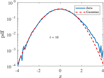
Figure 4: Numerical simulation of $10^{5}$ realizations of winding in an annulus with inner radius $a=1/2$ and outer radius $b=2$, with vortex strength $\beta=1$. Compared to the unbounded cases, the convergence in $t$ is very rapid. Note that there is a slight asymmetry biased in the direction of the drift, which is not captured at this order of the expansion.

Appendix A Small-$k_{\mu}$ asymptotics of integral

We justify that the $\mu$ integral in Eq. 24 is dominated by small $k_{\mu}$ when $t\rightarrow\infty$, or equivalently when $\lambda\rightarrow 0$. By symmetry, we need only consider the case where $\mu>0$. For some fixed small $\delta>0$, we will show that as $\lambda\rightarrow 0$,

(62a) $$\mathrm{I}_{<\delta} =\left\lvert\int_{0}^{\delta}{\mathrm{e}}^{\mathrm{i}\mu\theta}\,Z_{k_{\mu}}(\lambda r,\lambda a)\,Z_{k_{\mu}}(\lambda r_{0},\lambda a)\mathop{}\!\mathrm{d}\mu\right\rvert=\mathcal{O}\!\left(1/\log\lambda^{-1}\right),$$

(62b) $$\mathrm{I}_{>\delta} =\left\lvert\int_{\delta}^{\infty}{\mathrm{e}}^{\mathrm{i}\mu\theta}\,Z_{k_{\mu}}(\lambda r,\lambda a)\,Z_{k_{\mu}}(\lambda r_{0},\lambda a)\mathop{}\!\mathrm{d}\mu\right\rvert=\mathcal{O}\!\left(\lambda^{\sqrt{2}\delta}/\log\lambda^{-1}\right).$$

Hence, the ratio $\mathrm{I}_{<\delta}/\mathrm{I}_{>\delta}\rightarrow\infty$ as $\lambda\rightarrow 0$ and the integral is dominated by small $\mu<\delta$. In other words, we show that for any fixed small $\delta>0$, there is a $\lambda$ small enough to ensure that the $\mu$-integral is dominated by $\mu<\delta$.

For small $\lambda$ we can use the expansion Eq. 26 for $Z_{k_{\mu}}(\lambda r_{0},\lambda a)$. Since $k_{\mu}=\sqrt{\mu^{2}+\mathrm{i}\beta\mu}$ with $\beta>0$ and $r_{0}>a$, we have, as $\mu\rightarrow\infty$,

(63) $$k_{\mu}\sim\mu+\mathrm{i}\beta/2,\qquad\Gamma(1+k_{\mu})\sim\sqrt{2\pi k_{\mu}}\,(k_{\mu})^{k_{\mu}}{\mathrm{e}}^{-k_{\mu}},\qquad\bigl{\lvert}(r_{0}/a)^{k_{\mu}}\bigr{\rvert}\rightarrow\infty,$$

the second of which is Stirling’s approximation. Hence, one of the terms in the denominator of Eq. 26 is

(64) $$(\lambda a/2)^{-k_{\mu}}\Gamma(1+k_{\mu})\sim\sqrt{2\pi k_{\mu}}\,(2k_{\mu}/\lambda a{\mathrm{e}})^{k_{\mu}}$$

whose magnitude goes to $\infty$ rapidly with increasing $\mu$. Euler’s reflection formula $\Gamma(z)\Gamma(1-z)=\pi/\sin(\pi z)$ allows us to show

(65) $$\lvert(\lambda a/2)^{k_{\mu}}\Gamma(1-k_{\mu})\rvert\lesssim\frac{\pi}{\sinh(\pi\beta/2)}\,\left\lvert\frac{(\lambda a/2)^{k_{\mu}}}{\Gamma(k_{\mu})}\right\rvert\rightarrow 0.$$

The final term in the denominator of Eq. 26 is

(66) $$\lvert 2\pi k_{\mu}\tan(\pi k_{\mu}/2)\rvert\lesssim 2\pi\lvert k_{\mu}\rvert\coth(\pi\beta/4)$$

which does not go to zero as $\mu\rightarrow\infty$, but can be neglected compared to the square of Eq. 64. Moreover, it can also be neglected compared to the next-order asymptotic improvement of Stirling’s formula; since it is the only negative term, we will obtain an asymptotic lower bound. Referring back to Eq. 26, there exists $N$ large enough such that whenever $\mu>N>\delta$, we have $\bigl{\lvert}(r_{0}/a)^{k_{\mu}}+(r_{0}/a)^{-k_{\mu}}\bigr{\rvert}\lesssim 2\bigl{\lvert}(r_{0}/a)^{k_{\mu}}\bigr{\rvert}$ for $r_{0}>a$, and

$$\sqrt{[(\lambda a/2)^{k_{\mu}}\Gamma(1-k_{\mu})+(\lambda a/2)^{-k_{\mu}}\Gamma(1+k_{\mu})]^{2}-2\pi k_{\mu}\tan(\pi k_{\mu}/2)}\\ \geq\bigl{\lvert}\sqrt{2\pi}\,(k_{\mu})^{1/2}(2k_{\mu}/\lambda a{\mathrm{e}})^{k_{\mu}}\bigr{\rvert}.$$

Putting these together, we have the asymptotic bound

(67) $$\lvert Z_{k_{\mu}}(\lambda r_{0},\lambda a)\rvert\leq\frac{2}{\sqrt{2\pi\lvert k_{\mu}\rvert}}\bigl{\lvert}(\lambda r_{0}{\mathrm{e}}/2k_{\mu})^{k_{\mu}}\bigr{\rvert}$$

for $\mu>N$.

We thus have the estimate

$$\int_{N}^{\infty}\left\lvert Z_{k_{\mu}}(\lambda r,\lambda a)\,Z_{k_{\mu}}(\lambda r_{0},\lambda a)\right\rvert\mathop{}\!\mathrm{d}\mu \leq\frac{2}{\pi}\int_{N}^{\infty}\left\lvert\frac{\lambda^{2}rr_{0}{\mathrm{e}}^{2}}{4k_{\mu}^{2}}\right\rvert^{\Re(k_{\mu})}\!\frac{1}{\lvert k_{\mu}\rvert}\mathop{}\!\mathrm{d}\mu$$

$$\leq C_{1}(\beta)\int_{N}^{\infty}\left\lvert\frac{\lambda^{2}rr_{0}{\mathrm{e}}^{2}}{4\mu^{2}}\right\rvert^{\mu}\,\frac{\!\mathop{}\!\mathrm{d}\mu}{\mu}$$

$$\leq C_{1}(\beta)\int_{\delta}^{\infty}\left\lvert\frac{\lambda^{2}rr_{0}{\mathrm{e}}^{2}}{4\delta^{2}}\right\rvert^{\mu}\,\frac{\!\mathop{}\!\mathrm{d}\mu}{\mu}$$

$$\leq C_{2}(\delta,\beta,r,r_{0})\frac{\lambda^{2\delta}}{\log\lambda^{-1}},$$

where in the last step we used the asymptotic form for the incomplete Gamma function. The real part of $k_{\mu}$ is bounded from below for all $\mu\geq 0$:

(68) $$\Re(k_{\mu})=(\mu^{2}(\mu^{2}+\beta^{2}))^{1/2}\,\cos\left(\tfrac{1}{2}\arg(\mu+\mathrm{i}\beta)\right)\geq\mu/\sqrt{2}.$$

On the interval $\mu\in[\delta,N]$, since $\mu$ is bounded the term $(\lambda a/2)^{-k_{\mu}}$ dominates for small $\lambda$ in the denominator of Eq. 26; therefore we can bound the integral Eq. 62b as

$$\mathrm{I}_{>\delta} \leq\int_{\delta}^{\infty}\left\lvert Z_{k_{\mu}}(\lambda r,\lambda a)\,Z_{k_{\mu}}(\lambda r_{0},\lambda a)\right\rvert\mathop{}\!\mathrm{d}\mu$$

$$\leq C_{3}(\delta,\beta,r,r_{0})\int_{\delta}^{N}\lambda^{2\Re(k_{\mu})}\mathop{}\!\mathrm{d}\mu+\int_{N}^{\infty}\left\lvert Z_{k_{\mu}}(\lambda r,\lambda a)\,Z_{k_{\mu}}(\lambda r_{0},\lambda a)\right\rvert\mathop{}\!\mathrm{d}\mu$$

$$\leq C_{3}(\delta,\beta,r,r_{0})\int_{\delta}^{N}\lambda^{\sqrt{2}\mu}\mathop{}\!\mathrm{d}\mu+\int_{N}^{\infty}\left\lvert\frac{\lambda^{2}rr_{0}{\mathrm{e}}^{2}}{4k_{\mu}^{2}}\right\rvert^{\Re(k_{\mu})}\!\frac{1}{\lvert k_{\mu}\rvert}\mathop{}\!\mathrm{d}\mu$$

$$\leq C_{4}(\delta,\beta,r,r_{0})\frac{\lambda^{\sqrt{2}\delta}}{\log\lambda^{-1}}+C_{2}(\delta,\beta,r,r_{0})\frac{\lambda^{2\delta}}{\log\lambda^{-1}}$$

$$=\mathcal{O}\!\left(\lambda^{\sqrt{2}\delta}/\log\lambda^{-1}\right).$$

Finally we show (62a). By choosing $\delta$ small enough and noting that $a$, $r$, $r_{0}$, $\theta$ are all fixed, a small-$\mu$ approximation can be applied to go from Eq. 26 to Eq. 27, and then

(69) $$Z_{k_{\mu}}(\lambda r_{0},\lambda a)\sim\frac{\cosh(k_{\mu}\log(r_{0}/a))}{\cosh(k_{\mu}\log(\lambda\and/2))}\sim\operatorname{sech}(\sqrt{\beta\mu/2}\,(1+\mathrm{i})\log(\lambda\and/2)).$$

Therefore, denoting $c=\sqrt{\beta/2}\log(2/\lambda\and)$, we have

$$\mathrm{I}_{<\delta} \sim\left\lvert\int_{0}^{\delta}\operatorname{sech}^{2}(\sqrt{\beta\mu/2}\,(1+\mathrm{i})\log(\lambda\and/2))\mathop{}\!\mathrm{d}\mu\right\rvert$$

$$=\frac{(1-\mathrm{i})c\sqrt{\delta}\tanh((1-\mathrm{i})c\sqrt{\delta})+\mathrm{i}\log(\cosh((1-\mathrm{i})c\sqrt{\delta}))}{c^{2}}$$

$$\sim\frac{c\sqrt{\delta}-\pi/2+\mathrm{i}\log(\sqrt{2}/2\sin(c\sqrt{\delta}+\pi/4)}{c^{2}}$$

(70) $$=\mathcal{O}\!\left(1/\log\lambda^{-1}\right).$$

Appendix B Small-$k_{\mu}$ asymptotics of $\mathrm{I}_{k_{\mu}}(t)$

In this Appendix we derive an asymptotic form for $\mathrm{I}_{k_{\mu}}(t)$ defined by Eq. 30, valid for small $k_{\mu}$ and $t\rightarrow\infty$. We drop the $\mu$ subscript on $k_{\mu}$ to lighten the notation, since we only need to know that $k$ is small.

Expanding $Z_{k}(\lambda r,\lambda a)$ in Eq. 30 according to Eq. 28, we have

(71) $$\mathrm{I}_{k}(t)\sim\int_{a}^{\infty}\int_{0}^{\infty}{\mathrm{e}}^{-\lambda^{2}t}\left(J_{k}(\lambda r)-Y_{k}(\lambda r)\,\frac{(\lambda\and/2)^{k}\sin{\pi k}}{(\lambda\and/2)^{k}+(\lambda\and/2)^{-k}}\right)\\ \times\operatorname{sech}(k\log(\lambda\and/2))\,\lambda r\mathop{}\!\mathrm{d}\lambda\mathop{}\!\mathrm{d}r.$$

Now make the change of variable

(72) $$\lambda=y/L,\qquad r=Lz/y,\quad\text{where}\quad L(t)=\sqrt{t},$$

in $\mathrm{I}_{k}(t)$. We can expand $\operatorname{sech}(k\log(\and y/2L))$ when $(\and y/2L)<1$, since $\Re(k)>0$:

(73) $$\operatorname{sech}(k\log\tfrac{\and y}{2L})=2\sum_{n=0}^{\infty}(-1)^{n}\left(\frac{\and y}{2L}\right)^{(2n+1)k}\,.$$

The condition $(\and y/2L)<1$ is satisfied since Eq. 71 is effectively truncated at finite $y$, due to the factor ${\mathrm{e}}^{-y^{2}}$, so essentially by dominated convergence

$$\mathrm{I}_{k}(t)=2\sum_{n=0}^{\infty}(-1)^{n}\left(\frac{\and}{2L}\right)^{(2n+1)k}\int_{0}^{\infty}\int_{ay/L}^{\infty}{\mathrm{e}}^{-y^{2}}y^{(2n+1)k-1}J_{k}(z)\,z\mathop{}\!\mathrm{d}z\mathop{}\!\mathrm{d}y\\ -2\sin{\pi k}\sum_{n=0}^{\infty}(-1)^{n}(n+1)\left(\frac{\and}{2L}\right)^{(2n+3)k}\int_{0}^{\infty}\int_{ay/L}^{\infty}{\mathrm{e}}^{-y^{2}}y^{(2n+3)k-1}Y_{k}(z)\,z\mathop{}\!\mathrm{d}z\mathop{}\!\mathrm{d}y.$$

It can be shown that as $L\rightarrow\infty$

(74) $$\int_{0}^{\infty}\int_{ay/L}^{\infty}{\mathrm{e}}^{-y^{2}}y^{(2n+1)k-1}J_{k}(z)\,z\mathop{}\!\mathrm{d}z\mathop{}\!\mathrm{d}y\longrightarrow\tfrac{k}{2}\,\Gamma\left(\tfrac{2n+1}{2}k\right)$$

and

(75) $$\int_{0}^{\infty}\int_{ay/L}^{\infty}{\mathrm{e}}^{-y^{2}}y^{(2n+1)k-1}Y_{k}(z)\,z\mathop{}\!\mathrm{d}z\mathop{}\!\mathrm{d}y\longrightarrow\tfrac{k}{2}\,\Gamma\left(\tfrac{2n+1}{2}k\right)\cot\tfrac{\pi k}{2}$$

for $0<\Re(k)<2$, which is satisfied since $k$ is small. Hence,

(76) $$\mathrm{I}_{k}(t)=2\sum_{n=0}^{\infty}(-1)^{n}\left(\frac{\and}{2L}\right)^{(2n+1)k}\tfrac{k}{2}\,\Gamma\left(\tfrac{2n+1}{2}k\right)\\ -2\sin(\pi k)\cot(\pi k/2)\sum_{n=0}^{\infty}(-1)^{n}(n+1)\left(\frac{\and}{2L}\right)^{(2n+3)k}\tfrac{k}{2}\,\Gamma\left(\tfrac{2n+3}{2}k\right).$$

Since for small $k$,

(77) $$\frac{2n+1}{2}\,k\,\Gamma\left(\frac{2n+1}{2}k\right)\sim 1,\qquad\sin(\pi k)\cot(\pi k/2)\sim 2,$$

we have,

(78) $$\mathrm{I}_{k}(t)\sim 2\sum_{n=0}^{\infty}(-1)^{n}\tfrac{1}{2n+1}\left(\frac{\and}{2L}\right)^{(2n+1)k}-4\sum_{n=0}^{\infty}(-1)^{n}\tfrac{n+1}{2n+3}\left(\frac{\and}{2L}\right)^{(2n+3)k}.$$

Reindexing the second sum then allows us to combine the sums to obtain

$$\mathrm{I}_{k}(t) \sim 2\sum_{n=0}^{\infty}(-1)^{n}\left(\frac{\and}{2L}\right)^{(2n+1)k}$$

(79) $$=\operatorname{sech}(k\log(\and/2L)).$$

which is Eq. 31.

Appendix C Free Brownian motion revisited

In this Appendix we use our results to slightly improve the normalizer used by Grosberg & Frisch [8] for the free Brownian motion cases $\beta=0$ (i.e., without tangential drift), which makes the normalizer asymptotically correct to $\mathcal{O}\!\left(1\right)$ for large $t$. Numerical simulations confirm a modest improvement.

For the case of winding around a point, we already derived in Eq. 22 the correction to Spitzer and Grosberg & Frisch’s result,

(80) $$\frac{2\Theta(t)}{\log(4t/r_{0}^{2}{\mathrm{e}}^{\gamma})}\xrightarrow{\enskip d\enskip}X,\qquad p_{X}(x)=\frac{1}{\pi}\frac{1}{1+x^{2}}\,.$$

The only difference is the ${\mathrm{e}}^{\gamma}$ factor in the normalizer. Similarly, the calculation in Section 4 for $\beta=0$ can be shown to give

(81) $$\frac{2\Theta(t)}{\log(4t/a^{2}\,{\mathrm{e}}^{\gamma})}\xrightarrow{\enskip d\enskip}X,\qquad p_{X}(x)=\tfrac{1}{2}\operatorname{sech}(\pi x/2).$$

The reason for the missing factor in the normalizer of Grosberg & Frisch can be traced to their use of the asymptotic form Eq. 14 for the $J_{k_{\mu}}(\lambda r)$ in Eq. 13. This renders the $r$ integral divergent at infinity. To remedy this, the authors truncate the integral at $r\sim\sqrt{4t}$, which is reasonable but in doing so they lose a constant factor of ${\mathrm{e}}^{\gamma}$ in the normalizer. Our approach avoids this and is asymptotically valid.

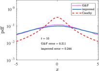
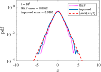
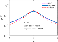
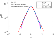
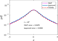
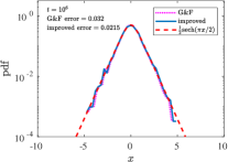
Figure 5: Numerical simulations without drift ($\beta=0$). The left column shows $10^{5}$ realizations for a point-like obstacle with $r_{0}=1$. The right column is for $10^{4}$ realizations of winding around a disk of radius $a=2$. The error is the $\mathrm{L}^{2}$ norm of the difference between the data and the limit distribution in each case.

We compare the corrected forms Eqs. 80 and 81 to a normalizer without the factor ${\mathrm{e}}^{\gamma}$ for numerical simulations in Fig. 5. The improvement is marginal and can only be seen for large times. Nevertheless, we include it here for completeness and rigor.

References

- [1] C. Bélisle, Windings of random walks, Ann. Prob., 17 (1989), pp. 1377–1402.
- [2] C. M. Bender and S. A. Orszag, Advanced Mathematical Methods for Scientists and Engineers, McGraw–Hill, New York, 1978.
- [3] M. A. Berger, The random walk winding number problem: convergence to a diffusion process with excluded area, J. Phys. A, 20 (1987), pp. 5949–5960.
- [4] M. A. Berger and P. H. Roberts, On the winding number problem with finite steps, Adv. Appl. Prob., 20 (1988), pp. 261–274.
- [5] A. Comtet, J. Desbois, and C. Monthus, Asymptotic winding angle distributions for planar Brownian motion with drift, J. Phys. A, 26 (1993), p. 5637.
- [6] B. Drossel and M. Kardar, Winding angle distributions for random walks and flux lines, Phys. Rev. E, 53 (1996), pp. 5861–5871.
- [7] X. Geng and G. Iyer, Long time asymptotics of heat kernels and Brownian winding numbers on manifolds with boundary, Apr. 2018, https://arxiv.org/abs/1804.00368.
- [8] A. Grosberg and H. Frisch, Winding angle distribution for planar random walk, polymer ring entangled with an obstacle, and all that: Spitzer-Edwards-Prager-Frisch model revisited, J. Phys. A, 36 (2003), pp. 8955–8981.
- [9] T. Kato, Perturbation theory for linear operators, vol. 132, Springer Science & Business Media, 2013.
- [10] H. Lamb, Hydrodynamics, Cambridge University Press, Cambridge, U.K., 6 ed., 1932.
- [11] J.-F. Le Gall and M. Yor, Étude asymptotique de certains mouvements browniens complexes avec drift, Probab. Th. Rel. Fields, 71 (1986), pp. 183–229.
- [12] P. Messulam and M. Yor, On D. Williams’ “pinching method” and some applications, J. London Math. Soc. (2), 26 (1982), pp. 348–364.
- [13] J. Rudnick and Y. Hu, The winding angle distribution for an ordinary random walk, J. Phys. A, 20 (1987), pp. 4421–4438.
- [14] F. Spitzer, Some theorems concerning -dimensional Brownian motion, Trans. Amer. Math. Soc., 87 (1958), pp. 187–197.
- [15] E. Toby and W. Werner, On windings of multidimensional reflected Brownian motion, Stochastics and Stochastics Reports, 55 (2001), pp. 315–327.
- [16] S. Vakeroudis, On the windings of complex-valued Ornstein–Uhlenbeck processes driven by a Brownian motion and by a stable process, Stochastics, 87 (2015), p. 2015.