Evaluation of spike sorting algorithms: Simulations and application to human Subthalamic Nucleus recordings

Abstract

An important prerequisite for the analysis of spike synchrony in extracellular recordings is the extraction of single unit activity from the recorded multi unit signal. To identify single units (SUs), potential spikes are first extracted and then separated with respect to their potential neuronal origins (’spike sorting’). However, different sorting algorithms yield inconsistent unit assignments which seriously influences the subsequent analyses of the spiking activity.

To evaluate the quality of spike sortings performed with different algorithms (K-Means, Valley-Seeking, Expectation Maximization) offered by a standard commercial spike sorter (’Plexon Offline Sorter’) we first apply these algorithms to experimental data (ED), namely recordings in the Subthalamic Nucleus of patients with Parkinson’s disease, obtained during Deep Brain Stimulation surgery. Since this procedure leaves us unsure about the best sorting method for the ED we then apply all methods again to artificial data (AD) with known ground truth (GT). AD consists of pairs of SUs and perturbation signals embedded in the background noise adapted to mimic the ED. We generate four AD sets which differ in the similarity of embedded SU shapes.

The spike sorting evaluation is performed in terms of the influence of the respective methods on the SU assignments (e.g., number of units) and its effect on the resulting firing characteristics (e.g., firing rates). We find a high variability in the sorting results obtained by different algorithms that increases with SU shape similarity. We also find significant differences in the resulting firing characteristics of the ED. We conclude that Valley-Seeking produces the most accurate results if the identification of perturbation signals (i.e., artifacts) as unsorted events is important. If the latter is less important (’clean’ data) K-Means is a better option. Our results strongly argue for the need of standardized validation procedures for spike sorting based on GT data. The recipe suggested here is simple enough to become a standard procedure. It provides a good basis for the evaluation of spike sorting results in order to ensure reliability and reproducibility.

1 Introduction

The decomposition of extra-cellular multi unit recordings into single unit (SU) activity is a prerequisite for studying neuronal activity patterns [6, 10, 32, 59, 64]. The assignment of spikes to individual neurons based on the similarity of their spike shapes is a method commonly referred to as spike sorting [44, 36, 45]. It is composed of three principal steps. First, the spikes are extracted from the high-pass filtered raw signal. Second, salient features of each spike waveform are identified. A common method to automatically extract such features is the principal component analysis [36, 44]. Third, a sorting algorithm assigns spikes to putative single neuronal units using the extracted features. Many such spike sorting algorithms are available [36, 44, 45, 51, 7, 66] but they typically provide inconsistent results for the same data set [4, 30, 62]. Such differences in the sorting results affect the subsequent spike train analyses [4, 43, 59]. Therefore, a major challenge is to identify an appropriate spike sorting algorithm for a given data set, considering also its impact on the subsequent analysis [36, 59].

Extracellular recordings from the Subthalamic Nucleus (STN) of patients with Parkinson’s Disease (PD), obtained during Deep Brain Stimulation (DBS) surgery provide important information about pathological activity patterns. The analysis of the corresponding SU activity contributes to identify and localize pathological patterns, e.g., helping to improve the positioning of the stimulation electrode [27].

Besides common spike sorting problems such as bursting activities and overlapping spikes [36, 44], or waveform changes induced by an electrode drift, the separation of SUs in human STN data is particularly challenging [30]. Microelectrode recordings from brain areas densely packed with neurons, such as the STN [20], contain spikes from a large number of neurons. The overall recording time is restricted to only a few minutes per recording site since the surgery is exhausting and the patients have to stay awake. The short recording time does not allow to wait for stabilization of tissue and electrode. In contrast, animal studies allow for longer recordings so that it is possible to account for initial stabilization [47]. Also, simultaneous intra- and extracellular recordings for calibration can be performed in animal studies [21] but this is not feasible during DBS surgery. Another advantage in animal studies is the usage of 4-wire close-by electrodes (i.e., tetrodes) or even polytrodes [51, 50]. The resulting recordings generally enable a more accurate spike sorting because one neuron is registered at different wires allowing for triangulation [21, 51, 66, 33, 5]. In contrast, human DBS recordings are typically performed with up to five single-wire electrodes [39], typically inserted using a “Ben-gun” configuration [14, 48, 19, 40]. These electrodes have a maximum diameter of 1 mm with a distance of 2 mm. Thus, the insertion causes a considerable initial tissue movement and the spikes of one neuron are detected on one electrode only.

A few comparative spike sorting frameworks for human STN recordings have been introduced [6, 30, 62]. Wild et al. [62] compares three widely used open source sorting toolboxes (WaveClus [46], KlustaKwik [21], and OSort [52]) by applying them to artificial data with some STN characteristics. They conclude that WaveClus yields the best results, but does not perform optimally. Knieling et al. [30] compares a new approach to sort STN spikes to Osort and WaveClus, using the artifical data from [62]. However, to our knowledge, there is no comparative study using both artificial data and STN recordings.

The above studies concentrate on open source spike sorting algorithms, whereas many studies recording from the human STN [41, 56, 64, 54, 29, 37, 55] use a commercially available software, the ’Plexon Offline Sorter’ OFS. Because of its frequent usage and relevance in the scientific community we focus our studies on the various sorting algorithms offered by the OFS (see Sec. 2.3). There are some comparative studies for spike detection and feature extraction [36, 1, 17, 65, 61], but less studies focus on clustering. Here, we concentrate on the comparison of the results obtained with the following cluster algorithms: Template Matching (TMS), K-Means (KM), Valley Seeking (VS), standard and t-distribution Expectation Maximization (StEM and TDEM, respectively). Varying the cluster algorithm, we use an identical detection procedure and the first two or three principal components (PCs) as features, since the number of PCs to be used for the sorting is another matter of debate [26].

Firstly, we apply all sorting algorithms to the experimental STN data (ED) recorded from PD patients. This enables us to depict the method-dependent differences in the ED sorting results (see Fig. 1) and to subsequently point out their considerable impact on the analysis of spike trains from real-world recordings. The evaluation of SU assignments and properties yield significant differences in the spike sorting results and suggests a seemingly best method. For a quantitative comparison, however, ground truth (GT) data are necessary, i.e., data with known SU assignments [31, 66, 62]. We therefore generate artificial data (AD) with known GT that include several features that are close to those of STN recordings. The spike sorting algorithms are then applied to the AD to evaluate their sorting quality. Based on this procedure, we are finally able to identify which methods work best under which circumstances.

2 Material and Methods

We first briefly describe the ED, followed by a description of the AD generation. Then, we explain the main steps of spike sorting and finally, we detail the comparison and validation of the results of different clustering algorithms.

2.1 Experimental Data

ED were recorded intraoperatively from six awake patients with tremor-dominant idiopathic PD undergoing STN-DBS surgery. The STN was localized anatomically with preoperative imaging and its borders were intraoperatively verified by inspection of multi unit spiking activity. Up to five combined micro-macro-electrodes recorded single cell activities and LFPs using the INOMED ISIS MER-system 2.4 beta, INOMED Corp., Teningen, Germany. Four of the electrodes were distributed equally on a circle with 2 mm distance from the central electrode using a Ben Gun electrode guide tool. ED were already analyzed in a previous study [13] which was approved by the local ethic committee. For more detailed information about the recording setup and recording procedures see [14, 48, 19, 40].

The microelectrodes had an impedance of around 1MΩ during each recording session. The signal was amplified by a factor of 20 000, band-pass filtered from 220 to 3000 Hz, using a hardware Bessel filter, and sampled at 25 kHz by a 12 bit A/D converter (+/- 0.2 V input range). Recording started 6 mm above the previously planned target point. The extracellular multi unit signals were recorded after moving the electrode closer to its target in 1 mm steps.

A total of 38 STN recoding traces from six awake PD patients at rest with one to four simultaneous microelectrode trajectories in different recording depths were analyzed. Some example sortings are shown in Fig. 1. The inclusion criteria for a data trace were a) a minimum length of 20 s, b) no drifts in background activity, c) spiking activity in the STN (based on visual inspection), and d) not exceeding the dynamic range of the A/D converter. The longest stable segment of a given trace was selected for further analysis; the first 2 s of each recording after electrode movement were discarded.

Figure 1: Exemplary spike sorting of human STN recordings. (A) Two distinct SUs and (B) several similar SUs that were extracted from two STN recordings (top traces in A and B) by amplitude thresholding (horizontal red line). Colored vertical lines below the continuous traces indicate time stamps of potential spikes. Extracted spike waveforms are shown on the left, the corresponding clustering in feature space on the right: colored dots represent spikes, US in gray.

2.2 Artificial data generation

A rigorous way to compare spike sorting methods is to test them on data sets with known GT, i.e., we know which of the spikes originate from which neuronal units. To this end, we generate AD by first selecting the two most distinct average spike waveforms from one ED trace. To enhance their differences, the larger one is multiplied with a factor of 1.1 so that it exhibits more pronounced peak amplitudes than given in the ED. We call the waveforms w1 and w2. We then linearly combine w1 and w2 to obtain spike pairs (u1,u2) whose similarity can be varied parametrically:

u1 $$=\lambda\qquad\;\;\cdot\text{w1}+\>(1-\lambda)\cdot\text{w2}$$ (1)

u2 $$=(1-\lambda)\cdot\text{w1}+\>\lambda\qquad\;\;\cdot\text{w2 $\quad\qquad$with $\lambda\in$$[0.5,1]$}$$

Thus, by varying $\lambda$ we create data sets with different degrees of similarity of the spike pairs (u1,u2), see Fig. 2A. For $\lambda=1$ we obtain u1=w1 and u2=w2 with u1 and u2 being most different. For $\lambda=0.5$, u1 and u2 are identical. We generate four AD sets, each with one spike pair (u1,u2) obtained for a certain value of $\lambda$ with $\lambda=1,0.8,0.7,0.6$. The corresponding data sets are called setI ($\lambda=1$, most distinct pair), setII, setIII and setIV ($\lambda=0.6,$ most similar pair). The hypothesis behind this choice is that it should be easier to distinguish distinct spikes than similar spikes.

The spike pairs are then added to background noise (Fig. 2B,C). To obtain the noise as realistic as possible, we generate it from the ED, using concatenated recording intervals without any spikes. We reshuffle the phase of the original noise so that the power spectrum is kept constant. The respective pairs of spikes (u1,u2) are added to the noise, each at a rate of 14 Hz as estimated from the ED, assuming a Poisson distribution. Each of the four generated data sets has a length of 40 s, sampled at 25 kHz resulting in approx. 500 spikes per unit. Refractory period violations (rpv, see Sec. 2.4.2) are corrected for by shifting the corresponding spikes of each SU in time (the second one is shifted forward by 1 to 50 time stamps depending on the closeness of the two spikes) until no more rpv are found.

Inspired by the difficulties that occur during sorting the ED, we additionally include the following challenges: We inject overlapping spikes from different SUs by inserting u1 spikes 10 to 22 time stamps (randomly chosen) after some randomly chosen u2 spikes (approx. 2.5% of the total number of spikes per trace as estimated from the ED) and vice versa. We then again correct for rpv. Moreover, we add in total approx. 100 so-called perturbation (pt) signals to each trace. These represent artifacts, e.g., noise originating from electrical equipment which may resemble spikes [24]. Perturbations are given by 8 sinusoidal functions (black lines in Fig. 2B). Each pt consists of one cycle of the following frequencies $f=1,0.75,0.5,0.25$ with respect to $T=1.52$ ms spike length, using a positive amplitude of either the peak amplitude of u2 or half of it. The negative peak amplitude is fixed to the minimum of the spike generated with $\lambda=0.5$. The corresponding insertion times are again Poisson distributed with a firing rate of 3.3 Hz as estimated from the ED. The aim is to investigate how different sorting methods deal with such perturbations. Ideally, pt signals should be left as unsorted events (US).

Figure 2: Artificial data generation. (A) Four pairs (solid and dashed curves) of artificial spikes that are very distinct (setI, blue), distinct (setII, cyan), similar (setIII, magenta), and very similar (setIV, violet). (B) Exemplary setI spike pair (u1,u2) added to the noise (100 spikes each). Thick light blue and green lines indicate the average spike waveforms of u1 and u2, respectively, black lines indicate perturbations (pt). (C) Simulated recording traces (black lines) with the corresponding ground truth spike times: Each trace contains one particular (u1,u2) pair as well as pts (green, blue and black markers, respectively).

We generate 10 realizations for each of the four AD data sets. The noise is identical for the four data sets within one realization (setI to setIV) but changes between the 10 realizations. After inserting potential spike events, i.e., u1, u2 and pts, into the noise, some threshold crossings vanish while some new crossings without a corresponding AD event emerge, e.g., due to possible overlaps between u1, u2 and pt. Therefore, the spike times of the GT are obtained as follows: (1) Calculation of the spike detection threshold, i.e., mean signal minus four times the standard deviation (SD) of the complete trace, identical for all sorting methods and identical to the procedure used for the ED (cf. Sec. 2.3). (2) Insertion of u1 spikes into the pure noise and detection of threshold crossings. (3) Repetition of step (2) for u2 and pt signals, respectively. When comparing the spike times in GT and sorting results we only consider threshold crossings that occurred after insertion and that have a corresponding AD event time stamp. We allow for deviations up to +/- 0.5 ms. AD were generated using Python2.7.

2.3 Spike detection and spike sorting

ED and AD are separated into SUs using spike sorting algorithms implemented in the ’Plexon Offline Sorter’ OFS (Offline SorterTM, Plexon Inc., Dallas, TX, USA). During a pre-processing step, artifacts (i.e., non-physiological events that may resemble spikes, e.g., some of the pts in the AD) were identified by visual inspection and removed. The spike detection threshold was set to minus four SD of the background noise [42]. After detection, 360 µs before and 1160 µs after threshold crossing were extracted, resulting in a total spike length of 1520 µs (38 time stamps). The spikes are aligned at the point of threshold crossing (see Fig. 2B).

Several features of the waveforms such as peak and valley amplitude, peak-valley distance, energy of the signal, and PCs were extracted. For the supervised ’manual’ sorting method TMS (see Sec. 2.3.1), all extracted features were used to visually identify the templates and thus the number of clusters, while the clustering itself uses the complete waveforms. For all other algorithms, clustering is solely based on the first two (2D) or three (3D) principal components. We apply the sorting algorithms TMS, KM, VS, StEM, and TDEM (the methods are described in the following subsections) to both AD and ED.

VS and TDEM (see Secs. 2.3.3 and 2.3.4) automatically determine the number of resulting clusters (unsupervised clustering) but contain method-specific parameters which were set to default values d (see Tab. 1). In addition, these methods were applied in combination with a parameter scan which optimizes the method-specific parameters (called VSS, TDEMS if used with a scan). During such a scan, a spike sorting algorithm runs repetitively for a wide range of parameter values (varied by step size $\Delta$) to identify and select the run that yields the best sorting quality based on cluster quality metrics, e.g., distances in feature space. TMS, KM, and StEM require user intervention. To enable unsupervised clustering, KM and StEM are only applied in combination with a parameter scan (KMS, StEMS) which automatically computes the appropriate number of clusters. Table 1 and Fig. 3 list the methods that are used with a scan, as well as the corresponding parameter ranges.

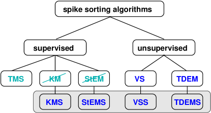
Figure 3: Spike sorting algorithms. Schematic overview of different sorting methods separated into originally supervised (cyan) and unsupervised algorithms (blue). Algorithms that are crossed out were only used in combination with a parameter scan (gray background) to enable unsupervised clustering.

Table 1: Methods used with a scan and their tunable parameters. The last column indicates the range of tested values, the step size $\Delta$, and the default value d if used without scan.

Method	Scanning parameter	Scanning range
KMS	#SUs	1-7 SUs
StEMS	#SUs	1-7 SUs
TDEM(S)	DOF multiplier	10 to 30, $\Delta$=5, d=10
VS(S)	Parzen multiplier	0.5 to 1.5, $\Delta$=0.2, d=1

In total, 13 different sorting approaches were applied to each data trace (TMS, VSS2(3)D, VS2(3)D, KMS2(3)D, StDEMS2(3)D, TDEMS2(3)D, TDEM2(3)D, cf. Fig. 3). We apply each method using the first two (2D) or three (3D) PCs, enabling a comparison of the corresponding performances. To investigate the effect of using a parameter scan, we apply each method with a method-specific parameter twice, once with parameter scan and once using its default value (see Tab. 1). After spike sorting, each threshold crossing event was either labeled as sorted into a cluster (SU) or left unsorted (US) if no clear assignment could be made. In the following subsections, we give more details on the spike sorting algorithms used in our study.

2.3.1 Template Matching sorting (TMS)

TMS is a supervised clustering algorithm, the number of clusters has to be predefined by the user. Based on various features (cf. Sec. 2.3) the user selects one waveform as template for each cluster. Then, the algorithm calculates the root-mean-square differences $D_{w}$ for all waveforms $w$ to these templates $t$: $D_{w}=\sqrt{1/N{\displaystyle{\textstyle\sum_{i=1}^{{\scriptstyle N}}(w_{i}-t_{i})^{2}}}}$, where $N$ is the number of time stamps per waveform. TMS identifies the template with minimum difference $D_{w}$ for each single waveform. If the minimum is smaller than a user defined value for the allowed variability, the particular waveform will be assigned to the cluster defined by this template.

2.3.2 K-Means clustering as Scan (KMS)

The K-Means algorithm requires the user to select a predefined number of clusters and the corresponding cluster centers which are here provided by the scanning algorithm. First, each sample point, i.e., each waveform in PC feature space is assigned to the nearest cluster center, based on Euclidean distances. Second, the cluster centers are recalculated using the center-of-gravity method [8, 18]. Steps one and two are repeated until convergence is reached, i.e., clusters centers are stable. Finally, outliers are removed: Based on mean ($\mu$) and SD of the distances of all sample points from their cluster center, a sample point is removed if it exceeds the outlier threshold, set to $\mu+2\cdot$SD. It is then left as US.

2.3.3 Valley Seeking (VS)

The VS algorithm is based on an iterative non-parametric density estimation [15, 67]. To subdivide the sample points (i.e., spikes) into exclusive clusters, the algorithm estimates their density in PC feature space using the Parzen approach [15], which estimates the appropriate kernel and its width for the best separation. VS calculates the number of neighbors of each sample point in a fixed local volume and determines the valleys in the density landscape. The critical radius R of the fixed volume is defined as $\text{{R}}=0.25\cdot\sigma\cdot\text{{PM}}$, where $\sigma$ is the SD of the distances of all samples to the overall center point, and PM is the Parzen multiplier, a user-defined parameter. A sample point becomes a seed point of a cluster if its number of neighbors exceeds a threshold. Then, initial clusters are formed by the seed points with the most neighbors. An iterative process classifies still unassigned sample points or leaves them unsorted. We run VS both with the PM default value, and using the scanning algorithm for PM (VSS).

2.3.4 Expectation Maximization algorithms (EM)

The standard EM (StEM) algorithm is an iterative, parametric approach that assumes that several Gaussian distributions underlie the distribution of sample points (i.e., spikes). The algorithm requires the user to select the number of Gaussians to be fitted and to define the initial cluster centers [15, 53]. To enable unsupervised clustering these are provided by the scanning algorithm. The algorithm starts by running the K-Means algorithm for the first assignment of sample points from which the initial Gaussian parameters are estimated. An iterative process optimizes these parameters until convergence of the Gaussian distributions to stable values. Each iteration consists of an expectation (E)-step that calculates the likelihood for each sample point to belong to each Gaussian, and a maximization (M)-step that maximizes the expected likelihood by optimizing the parameters [15, 53].

The t-distribution EM-algorithm (TDEM) differs from the StEM by fitting wide-tailed t-distributions instead of Gaussians. It has been shown that t-distributions yield a better fit to the underlying statistics of the waveform samples [57]. TDEM directly provides unsupervised clustering by starting with a large number of clusters and iteratively optimizing the likelihood function (assignment of samples to clusters) [57]. The shape of the t-distribution is determined by the degree of freedom (DOF) multiplier which depends on the sample size and controls the convergence properties [12, 57]. We run TDEM both with the DOF default value, and using the automatic scanning algorithm for DOF. In the Plexon implementation of these EM algorithms no events are left unsorted.

2.4 Evaluation of spike sorting results

Sorting results are characterized by the number of detected SUs and the number of unsorted events (US). The resulting means and SDs per data set are calculated by averaging over the 10 realizations for each AD set and the 38 ED recording traces, respectively.

2.4.1 Comparison with ground truth data

To evaluate the accuracy of the clustering algorithms, the resulting SUs were compared with a given GT. To quantify accordance with and deviations from the GT, we calculate the following numbers (cf. Fig. 5D and Fig. 8D):

TP

true positives, i.e., correctly assigned spikes: a waveform was given as element of a certain SU and was sorted into this SU.

FP

false positives (sorted), i.e., wrongly assigned (misclassified) spikes: a waveform was given as element of a certain SU but was sorted into another SU.

FN

false negatives, i.e., spikes wrongly left unsorted: a waveform was given as element of a certain SU but was left unsorted.

FPp

false positives (unsorted), i.e., wrongly assigned (misclassified) perturbations: a pt signal was classified as element of a certain SU.

TN

true negatives, i.e., correctly assigned perturbations: a pt signal was left unsorted.

Thus, a 100 % correct classification contains only TP and TN. For each data set sorted by a certain method, we count the corresponding hits (TP, TN) and misses (FP, FPp, FN) and normalize by the number of all events (spikes and pts) that are present in both GT and the corresponding sorting outcome. For each SU of the GT, we check which unit of the spike sorting outcome contains the most hits and then take this unit as correct. Therefore, we always find TP $>$ FP. Based on these numbers we calculate the following measures. The sensitivity describes how many spikes out of all spike events are correctly assigned: sensitivity = TP/(TP + FP + FN) while the specificity describes how many of the pts are correctly left unsorted: specificity = TN/(TN + FPp).

These analyses were performed using MATLAB (Mathworks Inc., Natick, U.S.A.). Differences in the general performance of the algorithms were evaluated by comparison to the GT values using the Wilcoxon rank sum test. Bonferroni’s correction was applied to adjust the significance level for multiple comparisons. To contrast the 2D with the 3D version of a method, we used direct comparisons (Wilcoxon rank sum test without Bonferroni’s correction), as well as for the comparison of running a method with a scan versus using the default parameter value.

2.4.2 Quality of spike sorting

We also assess the quality of our sorting results with the following evaluation measures: the percentage of refractory period violations (rpv), the isolation score (IS), and a measure characterizing the internal cluster distance (Di) [11, 23, 28, 10]. The amount of rpv indicates the degree of multi unit contamination in a given SU. We count the number of inter-spike intervals (ISIs) smaller than 2 ms divided by the total number of ISIs in this SU times 100. The IS compares the waveforms within one SU to all other potential spikes in the recording trace based on the normalized and scaled Euclidean distances of their time courses [28]. It provides an estimate of how well a SU is separated from all other potential spikes outside its cluster: IS=1 means well separated while IS=0 indicates overlapping clusters. It thus requires the existence of potential spikes outside a given cluster. Since EM methods do not account for US, we only calculate the IS when there are at least two SUs in a given trace. The internal cluster distance Di is also calculated if there is only one SU. This measure uses the first three PCs of each waveform. For each SU, we calculate the mean waveform and its mean euclidean distance (in reduced PC space) to all other spikes inside this cluster. For a consistent scaling behavior of the latter two quality measures we consider 1-Di so that high IS and high 1-Di values indicate well defined clusters.

2.4.3 Firing properties

To investigate the differences in the dynamical properties of the SUs we calculate the mean firing rate and the local coefficient of variation LV [56] in the ED. The LV characterizes the firing regularity of a SU:

$$LV=1/(n-1)\sum_{i=1}^{n-1}3(T_{i}-T_{i+1})^{2}/(T_{i}+T_{i+1})^{2},$$ (2)

where $T_{i}$ is the duration of the ith ISI and n the number of ISIs. LV values enable the following classification [56]: regular spiking for LV$\in[0,0.5]$, irregular for LV$\in]0.5,1]$, and bursty spiking for LV>1. For this analysis, only units with more than 80 spikes were taken into account to avoid outliers.

3 Results

We first present the evaluation of the results obtained by applying the 13 sorting algorithms to the STN recordings (ED), followed by an investigation of the impact of the sortings on the dynamical properties of the resulting SUs. The ED sorting evaluation leaves us in doubt about the best method. Therefore, we then evaluate the results of applying the identical methods to the AD which allows for an objective ground truth (GT) comparison. This procedure enables us to finally identify the best sorting methods.

3.1 Spike sorting of experimental data

We aim at sorting the ED under the additional constraint of identifying an unsupervised sorting algorithm that enables a fast, reliable and reproducible extraction of SUs. Our criteria for a successful sorting are: (1) all true spikes are detected and (2) non-spikes (i.e., artifacts) are not extracted as spikes but left unsorted. For a quantitative evaluation, we first sort the data using TMS, a manual sorting method that puts the user in complete control. According to our criteria it was performed with precise visual inspection aiming for clearly separated SUs that are free of artifacts and wrongly classified spikes. In search for an automatic sorting algorithm, we apply the following unsupervised methods offered by Plexon: VS and TDEM (both applied with parameter scan and default value, respectively, in 2D and 3D, respectively), as well as KMS and StEMS (both only applied with scan, in 2D and 3D, respectively). Some exemplary results are shown in Fig. 1. Here, we assume that the TMS sorting represents the GT, because TMS is a widely used method [52, 35, 47, 58], subjectively often perceived as the best sorting.

For a quantitative analysis we evaluate the number of detected SUs (Fig. 4A), the percentage of unsorted events US (Fig. 4B), and the percentage of refractory period violations rpv (Fig. 4C). The number of detected SUs is highly variable, depending on the sorting method. TMS and KMS3D detect on average two SUs, TDEM(S) detect on average significantly less units whereas VSS2(3)D yield significantly more units than TMS. EM methods do not account for US, they do not leave any spike unsorted. KMS methods yield the least US, followed by VS(S)2D while VS(S)3D and TMS show the highest percentage of US. TMS, all VS methods and KMS2(3)D result in less than 1.5% rpv. Methods that do not account for US yield more potential spikes per SU which results in a higher probability of rpv occurrences.

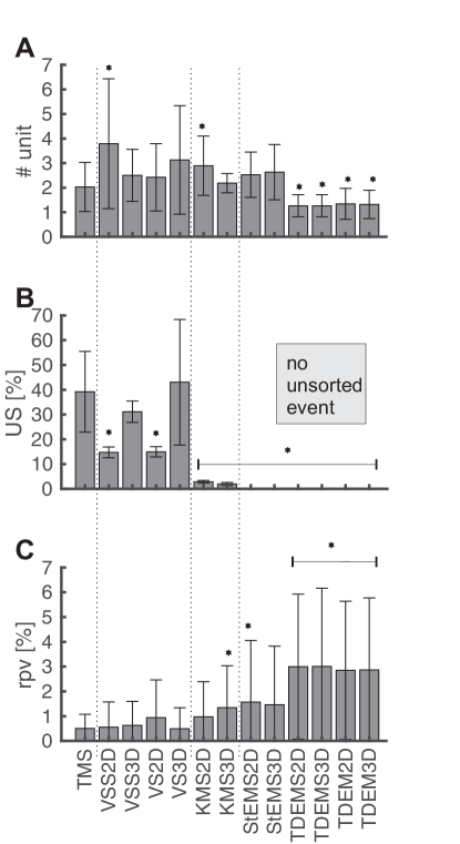
Figure 4: Evaluation of ED sorting results. (A, B, C) Bar plots of the average number of detected SUs (A), the percentage of US (B) and the percentage of rpv (C), in dependence of the sorting method. Shown are mean +/- SD of the 38 recording traces. Stars indicate a significant difference (p<0.0042 after Bonferroni correction) to the TMS results.

We now compare the assignments of the different sortings to the GT given by TMS using the terminology introduced in Sec. 2.4.1: TP, TN, FP, FPp and FN rates (Fig. 5D). Since TMS aims at ’clean’ SUs it results in a high TN rate of 39% and thus only 61% TP, see Fig. 5A. All other methods leave less events unsorted, resulting in lower TN (black) and accordingly higher FPp (dark gray) rates. They show a similar amount of misclassified spikes (FP, light blue) but clearly differ in terms of their FN (light gray), FPp and TN rates. EM methods, e.g., yield no TN but only FPp, since they do not allow for US, hence the high amount of rvp (cf. Fig. 4C). Compared to TMS (the assumed GT), TP rates are reduced for all other methods, the most for VS methods due to the high FN rates. KMS yield relatively high TP rates but very low TN rates because only a very few events are left unsorted (cf. Fig. 4B).

The sensitivity (i.e., percentage of TP relative to the total number of true spikes in TMS) and specificity (percentage of TN relative to the number of US in TMS) measures in Fig. 5B1 and Fig. 5B2 summarize these results. We aim at both a high sensitivity (i.e., correctly classified spikes) and a high specificity (events correctly left unsorted). In total, the sensitivity varies between 44% and 80% (Fig. 5B1), and the specificity between 0% and 64% (Fig. 5B2). All EM methods result in a high sensitivity, but zero specificity, because they do not account for US. KMS methods also yield a high sensitivity, but a low specificity. VS methods result in a high specificity combined with a rather low sensitivity. Combining these two measures, VSS3D seems to provide the best result, since it shows the highest sensitivity of all VS methods.

Figure 5: Evaluation of ED sorting results with GT (TMS) comparison. (A) Stacked bar plot showing the percentage of correct and wrong assignments of ED spikes in dependence of the sorting methods using TMS as GT reference: TP indicate correctly classified spikes, FP misclassified spikes, FN spikes left unsorted, FPp indicate US events of TMS that are classified as spikes, and TN indicates US events of TMS that are also left unsorted by the other methods. (B1, B2) Sensitivity and specificity measure in dependence of the sorting methods. Shown are mean +/- SD of all recording traces. (C1, C2) Cluster quality measures IS and (1-Di) applied to ED: each dot represents the value obtained for one SU in the 38 recording traces. Horizontal lines indicate the average over all SUs, vertical lines indicate the corresponding SD. (D) Summary of TP, TN, FP and FN notations and definition of sensitivity and specificity measures.

Fig. 5C1 and Fig. 5C2 asses the sorting quality from another perspective, independently of the assumed GT: The isolation score (IS) and the internal cluster distance (Di) indicate how well the resulting SUs are clustered (cf. Fig 1). For well separated clusters without artifact contamination, IS and 1-Di are close to one. The large vertical spread indicates a large variability for all methods, mostly due to the high variability in the #SU detected by each method, cf. Fig. 4A. TMS yields a rather low IS although the low percentage of rpv indicates a successful sorting (cf. Fig. 4C). The high IS values for TDEM methods do not indicate well defined clusters due to a high amount of rpv (cf. Fig. 4C). They are simply a consequence of the fact that the IS can only be calculated when there is more than one SU which is not often the case, cf. Fig. 4A. The Di measure considers all SUs and indeed indicates poorly defined clusters. KMS methods yield relatively high IS and 1-Di values and a reasonable amount of rpv. VS methods show relatively high 1-Di values but comparably low IS scores. Together with the high FN rate (Fig. 5A) this indicates that many spikes are left unsorted.

In summary, we find that VSS3D agrees best with the TMS results, suggesting that VSS3D is the best sorting method. However, a detailed comparison of the assignment of individual spikes indicates considerable differences: The FPp, FP, and FN rates for VSS3D sum up to approx. 40%. Other issues are the low IS score for both TMS and VSS3D, the higher TP rate for KMS compared to VSS3D, as well as the fact that we might loose a lot of true spikes when using TMS or VSS3D due to 39% US. Moreover, all VS and KMS methods detect more SUs compared to TMS. Tab. 2 in Sec. 5 lists more quantitative details. In the end, we are left with the suspicion that the subjective TMS sorting and thus VSS3D might, after all, not be the best methods to sort our data. In Sec. 3.3 we therefore apply all methods again to AD which provides an objectively given GT to compare with.

3.2 Impact of spike sorting methods on SU firing properties

To characterize the differences in the firing patterns of all detected SUs that result from using different sorting algorithms, we calculate the firing rate and the local coefficient of variation for each SU. Fig. 6A and Fig. 6B show the corresponding distributions obtained by binning and averaging across all STN recording traces. Each entry is averaged over all SUs identified in the ED. Fig. 6A shows clear discrepancies in the firing rate distributions. This is a consequence of the distinct number of SUs obtained from the different methods, as well as of the amount of US (cf. Fig. 4). SUs obtained with TMS and VS show lower frequencies (maximally up to 30 Hz), while KMS and StEM yield SUs with up to 40 Hz. SUs obtained with TDEM methods have the highest firing rates (60 Hz) since these methods detect mostly one SU and leave no US.

Figure 6: Variability in the ED firing statistics. Differences in firing patterns characterized by (A) firing rate and (B) local coefficient of variation LV. The color code indicates the number of detected SUs normalized to the total number of detected SUs per method (binned and averaged over all traces). Mean firing rate and mean LV (averaged over all SUs) are indicated by white dots. (C) Amount of SUs with regular (LV$<$0.5), irregular (0.5$\leq$LV$\leq$1.0) and bursty (LV$>$1.0) firing patterns.

Another characteristic property of spiking activity is the LV which quantifies the regularity in neuronal firing (Fig. 6B). We again observe method-dependent deviations, based on the variable number of SUs: the lower the number of detected SUs, the more regular are the subsequent spike trains. When classifying the SUs according to their LV value in regular (LV<0.5), irregular (0.5$\leq$LV$\leq$1.0), and bursty (LV>1) firing neurons [56, 38] we find clear differences (6C): TDEM methods yield more regular and less bursty SUs (less than 5%) whereas VS2(3)D methods result in less regular and more bursty SUs (up to 25%).

3.3 Spike sorting of artificial data

The ED results left us undecided concerning the best sorting method. In need of an objective GT we now evaluate the results of sorting artificially generated data, see Sec. 2.2. For the AD we know the correct spike and perturbation (representing artifacts to be left unsorted) assignments.

Fig. 7 presents the first part of the sorting results obtained for AD sets with varying spike pair similarity. For each set we again evaluate the resulting number of SUs (Fig. 7A), the percentage of US (Fig. 7B) and rpv (Fig. 7C). The GT is shown on the very left of the panels.

Figure 7: Evaluation of AD sorting results. Bar plots of the sorting results in dependence of the sorting methods (color coded spike pair similarity in setI to setIV): (A) average number of detected SUs, (B) percentage of events left unsorted, and (C) percentage of refractory period violations (rpv). Shown are mean +/- SD of the 10 realizations, stars indicate a significant difference compared to the GT values (p<0.039 after Bonferroni correction).

For setI and setII (distinct spike pairs), the number of resulting SUs is mostly quite similar and close to the GT. For setIII and setIV (similar spike pairs) all TDEM algorithms detect significantly fewer units, whereas StEMS methods find significantly more units, similar to KMS and VSS (Fig. 7A). These observations are similar to the corresponding ED results (cf. Fig. 4A).

EM algorithms do not account for US and KMS methods leave only a very few US while VS methods yield many more US than present in the GT (15% to 40% compared to 10%, see Fig. 7B). The percentage of US resulting from TMS is mostly close to the GT, only setIV yields more than 10% US due to a nearly impossible distinction between pts and spikes. The major difference to the ED results is the small amount of US in the GT: Here, US represent artifacts whereas the large amount of US in the ED are mostly spikes that were left unsorted because no clear assignment could be made, see Sec. 3.1.

Most methods induce a significant percentage of rpv (Fig. 7C). The percentage of rpv is larger the more similar the embedded spike pairs are, as it is more difficult to separate similar spikes which induces sorting errors. As observed for the ED, we find that methods that do not account for US result in a high percentage of rpv, e.g., TDEM methods with more than 3% rpv for setIII and setIV. In contrast, VS methods yield mostly less than 1% rpv.

Fig. 8A1 to A4 show the second part of the AD results: the TP, TN, FP, FPp and FN assignments made for the four sets. The 100% correct GT assignment consists of two parts: 90% TP, i.e., correctly classified spikes and 10% TN, i.e., pts that were correctly left unsorted. Concerning the spike events in setI, most methods perform quite well, yielding a TP rate close to 90%. Only VS(S) methods leave 8% (2D) to 15% (3D) of spikes unsorted which results in a comparably high FN and low TP rate. However, as expected from the ED results, VS(S) methods also correctly leave most pts unsorted (TN close to 10%). KMS, StEMS, and TDEMS yield generally high FPp and low FN rates: many pts are wrongly classified as spikes and only a few or no spikes are left unsorted. FN, FPp and TN rates change only slightly with increasing spike pair similarity (setI to setIV) since pts are identical in all sets. The number of misclassified spikes, however, clearly increases with increasing spike pair similarity: In setII, TDEM(S)3D already show 30% FP due to collapsing the spikes from two SUs into one SU while all other methods yield 2% to 6% FP (Fig. 8A2). For setIII, all TDEM methods yield approx. 45% FP while most other methods result in fewer FP (5% to 15%) and correspondingly higher TP rates (60% to 80%). Only VS3D yields less than 50% TP due to the relatively high percentage of 20% FN.

Figure 8: Evaluation of AD sorting results with GT comparison. (A1-A4) Stacked bar plots showing the average percentage of correct and wrong assignments of spikes and pts for the AD in dependence of the sorting methods: TP indicates correctly classified spikes, FP misclassified spikes, FN spikes wrongly left unsorted, FPp indicates pts wrongly classified as spikes, and TN pts correctly left unsorted (c.f. D). Stars indicate a significant difference to the GT values (p<0.039 after Bonferoni correction). (B1, B2) Sensitivity and specificity measures in dependence of the sorting methods. Shown are mean +/- SD of the 10 realizations. (C1, C2) Cluster quality measures IS and 1-Di in dependence of the sorting methods: each dot represents the value obtained for one SU. Horizontal lines indicate the average over all SUs in 10 realizations, vertical lines indicate the corresponding SD. The color code in B1, B2, C1, and C2 represents the spike pair similarity. (D) Summary of TP, TN, FP and FN notations and definition of sensitivity and specificity measures.

Fig. 8C1 and Fig. 8C2 show that the cluster quality measures IS and Di mostly reflect the results obtained by the above GT comparison: the more similar the spike pairs, the lower the TP rate and the average IS. This agreement holds only partially for the Di. If the number of identified SUs is large, the resulting clusters are small and naturally have a small internal distance, e.g., the large 1-Di values for VSS in setIV (Fig. 8C2, cf. Fig. 7A). Thus, IS and Di have to be considered in relation to the number of SUs. VS methods show relatively high 1-Di values but low TP rates, an effect of the high FN rates which bear less influence on the Di measure [28]. For the TDEM(S) methods applied to setII, however, the Di results match the TP rates better than the IS results.

We expected that using more PCs yields better results. However, the significant (p<0.05) differences in the percentage of US and TP between VS(S)2D and VS(S)3D indicate the opposite: the 2D results are closer to the GT. Still, VS(S)3D yield significantly less rpv compared to VS(S)2D, but this is simply the consequence of leaving many US. Similarly, some of the TDEM(S)2D results (#SU and TP rate for setII) are significantly closer to the GT than the TDEM(S)3D results. Therefore we conclude, that VS and TDEM work better in 2D as compared to 3D feature space.

The differences between the results obtained with and without automatic scan are inconsistent and only pertain to VS methods. For example, VSS3D versus VS3D yields mostly significantly (p<0.05) different values for #SUs, US and TP where the results obtained with scan are closer to the GT for #SU and US but without scan, the TP rates are closer to the GT. Thus, we see no advantage in applying an automatic parameter scan. Tab. 3 and Tab. 2 in Sec. 5 list more quantitative details on the comparative analysis of AD and ED.

Fig. 8B1 and Fig. 8B2 summarize our findings: the sensitivity (normalized TP rate) clearly decreases with increasing spike similarity, independently of the sorting method: the more similar a spike pair, the harder is the task to distinguish the spikes and to sort them into different units. For setIV, all sensitivity values are close to 50% indicating that the sorting task is so difficult that the success rates are bound to be close to chance level. However, there is no clear dependency of the specificity (normalized TN rate) on the task difficulty. Since EM methods do not account for US, their specificity is zero. As expected from the ED results, VS methods show a high specificity but their sensitivity is rather low. In contrast, KMS and TMS show again, as observed for the ED, a low specificity while their sensitivity is relatively high. For the AD, we conclude that KMS and VS(S)2D yield the best compromise between high sensitivity, i.e., many correctly classified spikes, and high specificity, i.e., many identified pts. Hence, the doubts about VSS3D being the best sorting method for the ED are justified. Fig. 9 shows the so-called success rate, i.e., the sum of TP and TN rates (filled circles) for AD sets II and III with 90% spikes and 10% pts. It shows that TMS and KMS are the most successful methods, followed by VS2D. The open circles are an estimate obtained via re-normalization with changed proportions for spikes (50%) and pts (50%). In this case VS methods show a higher success rate than KMS and TMS. Thus, the best method to sort the data depends on the amount of perturbations (i.e., artifacts) which are to be left unsorted.

Figure 9: AD sorting results in dependence of the amount of perturbations. Shown are the sum of TP and TN rate of the AD setII and setIII for the sorting methods that account for US events (GT is at one). Filled circles indicate the proportion given in the AD, i.e., 90% spikes and 10% pts. Open circles indicate an estimate calculated by re-normalization assuming 50% spikes and 50% pts. The color code represents the spike pair similarity.

4 Discussion

The classification of multi unit activity into SUs is an important prerequisite for many types of data analysis, e.g., neuronal correlations, spike-LFP phase coupling, or tuning properties of single cells. The sorting evaluation procedure described in this study is generally applicable. We provide a comparative analysis that depicts and characterizes the differences in the results of a selected set of sorting algorithms, applied to ED and AD with known GT, respectively. Comparing the results of the ED to the four AD sets we find that the task difficulty in the ED is most similar to setIII of the AD, i.e., a hard task due to similar spike shapes.

We evaluate sorting methods provided by the ’Plexon Offline Sorter’, a frequently used software package [41, 56, 64, 54, 29, 37, 55]. Aiming for an objective comparison without any user intervention, we focus on algorithms that either run with a given default parameter value or in combination with a parameter scan. We additionally use supervised TMS in order to contrast our results with this widely-used [52, 35, 47, 58] method. However, the user intervention in such supervised methods is time consuming, it inherently includes a human bias [63] and it typically requires a parameter optimization[62]. Therefore, we aim to identify the most appropriate unsupervised sorting method.

In agreement with [4, 62, 30] we show that the results obtained by using different sorting methods differ significantly, in both ED and AD. There are deviations in the number of detected SUs, in the percentage of US and rpv, as well as differences in the cluster quality measures. While the IS is typically used to select well isolated SUs [38, 28, 9] we here apply it to verify an augmented occurrence of well isolated SUs if the corresponding waveforms are distinct and thus easy to separate.

Most extracellular recordings (in particular STN data, see Sec. 1) contain perturbations, e.g., movement or speech artifacts. Therefore, it is a clear disadvantage of EM methods that they do not leave any event unsorted. Even though such perturbations are often removed during a preprocessing procedure (cf. Sec. 2.3), a considerable percentage is typically not identified. For example, approx. 8 out of 10% pts survived the preprocessing of our AD. Consequently, the resulting SUs of all EM methods are contaminated, resulting in high FPp rates. Among the EM methods, StEM yields the highest sensitivity and the fewest rpv. Hill et all. [22, 23] discuss that the assumption of Gaussian distributions in StEM may be inappropriate for spike clusters due to spike shapes varying with time. The latter can be caused by bursting activity which is a prominent feature in STN recordings [2, 27, 58, 6]. Still, StEM works comparably well for our data, possibly due to constant spike shapes during our short recording duration.

VS algorithms yield the most specific sorting results, they leave nearly all pts unsorted. Yet, all VS methods also leave a considerable amount of spikes unsorted which decreases their sensitivity. For the AD, only VS(S)2D methods provide a good compromise between specificity and sensitivity. A previous study [31] details that TDEM performs better than VS in clustering artificial data adapted to resemble extracellular recordings from a turtle’s retina. Our AD, however, explicitly contains perturbations. In such a complex case, as typical for STN data [36], the non-parametric approach taken in the VS(S)2D might provide an advantage because the valleys separating the SUs do not have to obey a specific parametric form [15, 23].

KMS is the most sensitive algorithm, only a few spikes are left unsorted and the amount of missclassifications is acceptable. Yet, it detects only a very few perturbation and thus has a low specificity. There is no significant difference between KMS2D and KMS3D.

At first sight, one expects that more information (i.e., 3D) yields a better performance but VS and TDEM perform better in 2D feature space than in 3D. The additional dimension may capture the variability in the background noise [36, 3] and thus lead to misclassifications.

Another important point for selecting an appropriate sorting method is the type of analysis that the user aims to perform with the resulting SUs. Missed spikes (FN), for example, reduce the significance of spike synchrony stronger than misclassified spikes (FP) [43]. Thus, for the analysis of neuronal correlation in STN recordings [41, 60] KMS is a better choice than VS. Another example are tuning curves, i.e., the distributions of neuronal firing rates with respect to a movement[16] or stimulus [25] direction. In this case, misclassified events (spikes, pts) can induce incorrect multimodal distributions while missed spikes lead to an underestimation of the true firing rates [23].

Typically, the average firing rates measured in the STN of Parkinson patients are reported to range from 25 Hz up to 50 Hz [38, 58, 9, 49]. We observe rates ranging from 14 Hz up to 39 Hz, purely depending on the sorting algorithm. Thus, we find lower rates than reported in the literature which can have several reasons: the specific disease type (tremor dominant versus akinetic-rigid), disease duration [49], as well as the exact recording place [9]. The method-dependent dispersion of average firing rate values observed here is 25 Hz which is identical to the rate dispersion reported in the literature. Similarly, the amount of regular, irregular, and bursty SUs strongly depends on the sorting method. Bursting SUs are a characteristic feature of STN recordings in PD patients [6, 38, 2, 34] and are reported to vary from 5% to 25% [6] or 15% to 34% [38], depending on the recording site. We find a similar amount of variability, namely 7% to 25% bursting SUs, ascribed to the sorting method.

In summary, different spike sorting approaches yield highly variable results. In order to recommend a sorting method we distinguish between two cases: ’clean’ and ’noisy’ data. With ’clean’ we mean that a first visual inspection of the data indicates that there are only a few artifacts and distorted spike shapes – or the given perturbations can easily be identified and removed otherwise. With ’noisy data’ we mean frequent perturbations that are difficult to identify and to remove. If the data is relatively clean we recommend to use the KMS method since it offers the highest success rate (Fig. 9) due to a high sensitivity (Fig. 8B1) and relatively well isolated clusters. If the data is particularly noisy and if missed spikes are less relevant for the subsequent analysis, VS(S)2D is probably a better choice. It combines a high specificity with an intermediate sensitivity (Fig. 8B1,B2) so that its success rate is higher in case of many aritifacts (Fig. 9) and yields very few rpv.

The procedure described here could generally serve as a pre-analysis step to select the appropriate sorting method for a specific data set: One first generates an AD set with known GT which is adapted to the experimental recordings. The sorting algorithms in question are then applied to the AD and the results are evaluated in relation to the GT. Finally, one selects the method with the best results and applies it to the experimental recordings. It is elementary enough to be generally applicable but yields results specific to the given data. Our results clearly show the importance of a careful spike sorting method selection.

5 Appendix

5.1 Quantitave sorting results analysis

We here present two additional tables (Tab. 2 and Tab. 3) that quantitatively summarize the sorting results of both ED and AD, focusing on setII and setIII of the AD as these are most relevant: the setI spike pair is more distinct and thus easier to distinguish than ED spikes while the setIV spike pair is so similar and hard to distinguish that any sorting can only approach chance level, see Fig. 8A4 and B1. Moreover, the majority of the ED evaluation results are close to the values obtained for setIII.

Table 2: Evaluation measures for AD and ED. Summary of evaluation measures of AD and ED sorting methods: average percentage of refractory period violations and isolation score for AD and ED. The first two columns pertain to setII and setIII of the AD. The last two columns show the average number of units and the average percentage of US in the ED.

Methods	AD: rpv [%]	IS	ED: rpv [%]	IS	#SU	%US
TMS	0.33 | 0.57	0.89 | 0.79	0.53	0.64	2.0	39.2
VSS 2D	0.29 | 0.63	0.87 | 0.78	0.61	0.58	3.8	14.8
VSS 3D	0.09 | 0.26	0.83 | 0.75	0.66	0.64	2.5	31.1
VS 2D	0.28 | 0.55	0.87 | 0.73	1.07	0.66	2.4	15.0
VS 3D	0.04 | 0.19	0.66 | 0.58	0.54	0.52	3.1	43.1
KMS 2D	0.68 | 1.26	0.89 | 0.80	1.12	0.72	2.9	2.9
KMS 3D	0.6 | 1.27	0.89 | 0.79	1.36	0.78	2.2	2.0

Table 3: Evaluation measures for AD. Summary of AD sorting results with GT comparison: average number of detected units, percentage of unsorted events, TN and TP rate. The two entries per column indicate the results of setII and setIII.

Methods	#SU	%US	%TN	%TP
GT	2 | 2	7.5|7.8	7.5| 7.8	92.5 | 92.2
TMS	2 | 2	6.2 | 9.4	2.6 | 3.2	84.7 | 73.5
VSS 2D	2 | 2	16.8 | 15.8	4.0 | 4.4	78.4 | 70.0
VSS 3D	2 | 2	28.8 | 29.4	4.8 | 5.2	68.0 | 60.6
VS 2D	2 | 2.3	16.0 | 16.9	3.9 | 4.5	79.0 | 65.1
VS 3D	3.2 | 3.3	32.1 | 35.0	4.8 | 5.5	55.2 | 46.4
KMS 2D	2 | 2.4	3.7 | 4.1	1.9 | 1.7	85.7 | 76.1
KMS 3D	2 | 2.3	3.5 | 3.8	1.8 | 1.7	85.6 | 76.0

Considering the ED results only, and assuming TMS as GT, VSS3D seems to be the best sorting method (Tab. 2): It yields 31% US, less than 1% rvp, a comparably high IS and the #SUs is close to the TMS value. However, this rating changes when considering the AD results. Overall, VS(S)2D yields the best specificity results, i.e., it leaves most pts unsorted and it yields the lowest amount of rpv among all supervised methods. The total amount of misclassified events (FPp+FP) is only 7% (setII) and 18% (setIII), see Fig.$\,\ref{figGT},$ but VS methods yield comparable high FN rates: they leave many spikes unsorted. In contrast, KMS2D yields the best sensitivity results and it misses only a very few spikes (FN$<$2%). However, the misclassification of events (FPp+FP) is higher than in VS(S)2D (10.9% for setII and 20.4% for setIII) and leads to a comparably high percentage of rpv.

6 Acknowledgments

This work was supported by Deutsche Forschungsgemeinschaft Grant 1753/3-1 Klinische Forschergruppe (KFO219, TP12), Deutsche Forschungsgemeinschaft Grant GR 1753/4-2 & DE 2175/2-1 Priority Program (SPP 1665), the Helmholtz Association through the Helmholtz Portfolio Theme Supercomputing and Modeling for the Human Brain (SMHB), and by the European Union’s Horizon 2020 research and innovation programme under grant agreement No. 720270 & 785907 (Human Brain Project SGA1 & SGA2). We thank Paul Chorely and Alexa Riehle for technical help and fruitful discussions. Tragically, Paul Chorely died before we were able to finish the manuscript.

7 References

References

- [1] D. A. Adamos, E. K. Kosmidis, and G. Theophilidis. Performance evaluation of PCA-based spike sorting algorithms. Computer Methods and Programs in Biomedicine, 91(3):232–244, 2008.
- [2] C. Beurrier, P. Congar, B. Bioulac, and C. Hammond. Subthalamic nucleus neurons switch from single-spike activity to burst-firing mode. The Journal of Neuroscience, 19(2):599–609, 1999.
- [3] C. M. Bishop. Pattern recognition and machine learning. Springer-Verlag New York, 2006.
- [4] E. N. Brown, R. E. Kass, and P. P. Mitra. Multiple neural spike train data analysis: state-of-the-art and future challenges. Nature Neuroscience, 7(5):456–61, may 2004.
- [5] G. Buzsáki. Large-scale recording of neuronal ensembles. Nature Neuroscience, 7(5):446–51, 2004.
- [6] O. K. Chibirova, T. I. Aksenova, A. L. Benabid, S. Chabardes, S. Larouche, J. Rouat, and A. E. P. Villa. Unsupervised Spike Sorting of extracellular electrophysiological recording in subthalamic nucleus of Parkinsonian patients. BioSystems, 79(1-3 SPEC. ISS.):159–171, 2005.
- [7] J. E. Chung, J. F. Magland, A. H. Barnett, V. M. Tolosa, A. C. Tooker, K. Y. Lee, K. G. Shah, S. H. Felix, L. M. Frank, and L. F. Greengard. A fully automated approach to spike sorting. Neuron, 95(6):1381 – 1394.e6, 2017.
- [8] J. Dai, X. Liu, Y. Yi, H. Zhang, J. Wang, S. Zhang, and X. Zheng. Experimental study on neuronal spike sorting methods. Proceedings of the 2008 2nd International Conference on Future Generation Communication and Networking, FGCN 2008, 2:230–233, 2008.
- [9] M. Deffains, P. Holland, S. Moshel, F. Ramirez de Noriega, H. Bergman, and Z. Israel. Higher neuronal discharge rate in the motor area of the subthalamic nucleus of Parkinsonian patients. Journal of Neurophysiology, 112(6):1409–20, 2014.
- [10] G. T. Einevoll, F. Franke, E. Hagen, C. Pouzat, and K. D. Harris. Towards reliable spike-train recordings from thousands of neurons with multielectrodes. Current Opinion in Neurobiology, 22(1):11–17, 2012.
- [11] M. S. Fee, P. P. Mitra, and D. Kleinfeld. Variability of extracellular spike waveforms of cortical neurons. Journal of Neurophysiology, 76(6):3823–33, 1996.
- [12] M. A. T. Figueiredo and A. K. Jain. Unsupervised learning of finite mixture models. Pattern Analysis and Machine Intelligence, IEEE Transactions, 24(3):381–396, 2002.
- [13] E. Florin, M. Himmel, C. Reck, M. Maarouf, A. Schnitzler, V. Sturm, G. R. Fink, and L. Timmermann. Subtype-specific statistical causalities in parkinsonian tremor. Neuroscience, 210:353–62, 2012.
- [14] E. Florin, C. Reck, L. Burghaus, R. Lehrke, J. Gross, V. Sturm, G. R. Fink, and L. Timmermann. Ten Hertz thalamus stimulation increases tremor activity in the subthalamic nucleus in a patient with Parkinson’s disease. Clinical Neurophysiology, 119(9):2098–2103, 2008.
- [15] K. Fukunaga. Statistical Pattern Pattern Recognition. Pattern Recognition, 22(7):833–834, 1990.
- [16] A. Georgopoulos, J. Kalaska, R. Caminiti, and J. Massey. On the relations between the direction of two-dimensional arm movements and cell discharge in primate motor cortex. Journal of Neuroscience, 2(11):1527–1537, 1982.
- [17] S. Gibson, J. W. Judy, and D. Markovic. Comparison of spike-sorting algorithms for future hardware implementation. Annual International Conference of the IEEE Engineering in Medicine and Biology Society. IEEE Engineering in Medicine and Biology Society. Conference, 2008:5015–5020, 2008.
- [18] G. A. Gregory A. Wilkin and X. Huang. K-Means Clustering Algorithms: Implementation and Comparison. In Proceeding of the Second International Multi-Symposium of Computer and Computational Sciences (IMSCCS 2007), August 13-15, 2007, The University of Iowa, Iowa City, Iowa, USA, pages 133–136, 2007.
- [19] R. E. Gross, P. Krack, M. C. Rodriguez-Oroz, A. R. Rezai, and A. L. Benabid. Electrophysiological mapping for the implantation of deep brain stimulators for Parkinson’s disease and tremor. Movement Disorders, 21(SUPPL. 14), 2006.
- [20] C. Hamani. The subthalamic nucleus in the context of movement disorders. Brain, 127(1):4–20, 2004.
- [21] K. D. Harris, D. A. Henze, J. Csicsvari, H. Hirase, and G. Buzsáki. Accuracy of tetrode spike separation as determined by simultaneous intracellular and extracellular measurements. Journal of Neurophysiology, 84(1):401–414, 2000.
- [22] D. Hill, D. Kleinfeld, and S. B. Mehta. Spike Sorting. In P. P. Mitra and H. Bokil, editors, In Observed Brain Dynamics, chapter Chapter 1, pages 1–17. Oxford Press, 2007.
- [23] D. N. Hill, S. B. Mehta, and D. Kleinfeld. Quality metrics to accompany spike sorting of extracellular signals. The Journal of Neuroscience, 31(24):8699–705, 2011.
- [24] P. M. Horton, A. U. Nicol, K. M. Kendrick, and J. F. Feng. Spike sorting based upon machine learning algorithms (SOMA). Journal of Neuroscience Methods, 160(1):52–68, 2007.
- [25] D. H. Hubel and T. N. Wiesel. Receptive Fields of Single Neurones in the Cat’s Striate Cortex. J. Physiol., 148:574–591, 1959.
- [26] E. Hulata, R. Segev, and E. Ben-Jacob. A method for spike sorting and detection based on wavelet packets and Shannon’s mutual information. Journal of Neuroscience Methods, 117(1):1–12, 2002.
- [27] W. D. Hutchison, R. J. Allan, H. Opitz, R. Levy, J. O. Dostrovsky, A. E. Lang, and A. M. Lozano. Neurophysiological identification of the subthalamic nucleus in surgery for Parkinson’s disease. Annals of Neurology, 44(4):622–628, 1998.
- [28] M. Joshua, S. Elias, O. Levine, and H. Bergman. Quantifying the isolation quality of extracellularly recorded action potentials. Journal of Neuroscience Methods, 163:267–282, 2007.
- [29] R. Kelley, O. Flouty, E. B. Emmons, Y. Kim, J. Kingyon, J. R. Wessel, H. Oya, J. D. Greenlee, and N. S. Narayanan. A human prefrontal-subthalamic circuit for cognitive control. Brain, 141(1):205–216, 2018.
- [30] S. Knieling, K. S. Sridharan, P. Belardinelli, G. Naros, D. Weiss, F. Mormann, and A. Gharabaghi. An Unsupervised Online Spike-Sorting Framework. International Journal of Neural Systems, page 1550042, 2016.
- [31] J. Kretzberg, T. Coors, and J. Furche. Comparison of valley seeking and T-distributed EM algorithm for spike sorting. BMC Neuroscience, 10(Suppl 1):P47, 2009.
- [32] A. A. Kühn, T. Trottenberg, A. Kivi, A. Kupsch, G. H. Schneider, and P. Brown. The relationship between local field potential and neuronal discharge in the subthalamic nucleus of patients with Parkinson’s disease. Experimental Neurology, 194(1):212–220, 2005.
- [33] B. Lefebvre, P. Yger, and O. Marre. Recent progress in multi-electrode spike sorting methods. Journal of Physiology Paris, 110(4), 2016.
- [34] R. Levy, J. O. Dostrovsky, A. E. Lang, E. Sime, W. D. Hutchison, and A. M. Lozano. Effects of apomorphine on subthalamic nucleus and globus pallidus internus neurons in patients with Parkinson’s disease. Journal of Neurophysiology, 86(1):249–260, 2001.
- [35] R. Levy, W. D. Hutchison, A. M. Lozano, and J. O. Dostrovsky. Synchronized neuronal discharge in the basal ganglia of parkinsonian patients is limited to oscillatory activity. The Journal of Neuroscience, 22(7):2855–2861, 2002.
- [36] M. S. Lewicki. A review of methods for spike sorting: the detection and classification of neural action potentials. Network, 9(4):R53–78, 1998.
- [37] W. J. Lipski, A. Alhourani, T. Pirnia, P. W. Jones, C. Dastolfo-Hromack, L. B. Helou, D. J. Crammond, S. Shaiman, M. W. Dickey, L. L. Hold, R. S. Turner, J. A. Fiez, and R. M. Richardson. Subthalamic Nucleus Neurons Differentially Encode Early and Late Aspects of Speech Production. Journal of Neuroscience, 38(24):5620–5631, 2018.
- [38] M. A. J. Lourens, H. G. E. Meijer, M. F. Contarino, P. van den Munckhof, P. R. Schuurman, S. A. van Gils, and L. J. Bour. Functional neuronal activity and connectivity within the subthalamic nucleus in Parkinson’s disease. Clinical Neurophysiology, 124(5):967–81, 2013.
- [39] B. L. McNaughton, J. O Keefe, and C. A. Barnes. The stereotrode: A new technique for simultaneous isolation of several single units in the central nervous system from multiple unit records. J Neurosci Methods, 8:391 – 397, 1983.
- [40] K. P. Michmizos and K. S. Nikita. Can we infer subthalamic nucleus spike trains from intranuclear local field potentials? In Can we infer Subthalamic Nucleus Spike Trains from Intranuclear Local Field Potentials?, pages 5476–5479, 2010.
- [41] A. Moran, H. Bergman, Z. Israel, and I. Bar-Gad. Subthalamic nucleus functional organization revealed by parkinsonian neuronal oscillations and synchrony. Brain, 131(12):3395–3409, 2008.
- [42] S. Mrakic-Sposta, S. Marceglia, M. Egidi, G. Carrabba, P. Rampini, M. Locatelli, G. Foffani, E. Accolla, F. Cogiamanian, F. Tamma, S. Barbieri, and A. Priori. Extracellular spike microrecordings from the subthalamic area in Parkinson’s disease. Journal of Clinical Neuroscience, 15(5):559–567, 2008.
- [43] A. Pazienti and S. Grün. Robustness of the significance of spike synchrony with respect to sorting errors. Journal of Computational Neuroscience, 21(3):329–42, 2006.
- [44] R. Q. Quiroga. Spike sorting. Scholarpedia, 2(12):3583, jan 2007.
- [45] R. Q. Quiroga. Spike sorting. Current Biology, 22(2):R45–R46, 2012.
- [46] R. Q. Quiroga, Z. Nadasdy, and Y. Ben-Shaul. Unsupervised spike detection and sorting with wavelets and superparamagnetic clustering. Neural Computation, 16(8):1661–87, 2004.
- [47] A. Raz, E. Vaadia, and H. Bergman. Firing patterns and correlations of spontaneous discharge of pallidal neurons in the normal and the tremulous 1-methyl-4-phenyl-1,2,3,6-tetrahydropyridine vervet model of parkinsonism. The Journal of Neuroscience, 20(22):8559–8571, 2000.
- [48] C. Reck, M. Maarouf, L. Wojtecki, S. J. Groiss, E. Florin, V. Sturm, G. R. Fink, A. Schnitzler, and L. Timmermann. Clinical outcome of subthalamic stimulation in Parkinson’s disease is improved by intraoperative multiple trajectories microelectrode recording. Journal of Neurological Surgery, 73(6):377–386, 2012.
- [49] M. S. Remple, C. H. Brandenham, C. C. Kao, P. D. Charles, J. S. Neimat, and P. E. Konrad. Subthalamic nucleus neuronal firing rate increases with parkinson’s desease progession. Movement Disorders, 26(9):1657–1662, 2011.
- [50] H. G. Rey, C. Pedreira, and R. Q. Quiroga. Past, present and future of spike sorting techniques. Brain Research Bulletin, 119:106–117, 2015.
- [51] C. Rossant, S. N. Kadir, D. F. M. Goodman, J. Schulman, M. L. D. Hunter, A. B. Saleem, A. Grosmark, M. Belluscio, G. H. Denfield, A. S. Ecker, A. S. Tolias, S. Solomon, G. Buzsaki, M. Carandini, and K. D. Harris. Spike sorting for large, dense electrode arrays. Nature Neuroscience, 19(4):634 – 641, 2016.
- [52] U. Rutishauser, E. M. Schuman, and A. N. Mamelak. Online detection and sorting of extracellularly recorded action potentials in human medial temporal lobe recordings, in vivo. Journal of Neuroscience Methods, 154(1-2):204–224, 2006.
- [53] M. Sahani. Latent Variable Models for Neural Data Analysis. Doctoral Dissetation, California Institute of Technology Pasadena, CA, USA, 1999.
- [54] L. E. Schrock, J. L. Ostrem, R. S. Turner, S. A. Shimamoto, and P. A. Starr. The Subthalamic Nucleus in Primary Dystonia: Single-Unit Discharge Characteristics. Journal of Neurophysiology, 102(6), 2009.
- [55] S. A. Shimamoto, E. S. Ryapolova-Webb, J. L. Ostrem, N. B. Galifianakis, K. J. Miller, and P. A. Starr. Subthalamic nucleus neurons are synchronized to primary motor cortex local field potentials in Parkinson’s disease. Journal of Neuroscience, 33(17):7220–7233, 2013.
- [56] S. Shinomoto, K. Shima, and J. Tanji. Differences in spiking patterns among cortical neurons. Neural Computation, 15(12):2823–2842, 2003.
- [57] S. Shoham, M. R. Fellows, and R. A. Normann. Robust, automatic spike sorting using mixtures of multivariate t-distributions. Journal of Neuroscience Methods, 127(2):111–122, 2003.
- [58] F. Steigerwald, M. Pötter, J. Herzog, M. Pinsker, F. Kopper, H. Mehdorn, G. Deuschl, and J. Volkmann. Neuronal Activity of the Human Subthalamic Nucleus in the Parkinsonian and Nonparkinsonian State. Journal of Neurophysiology, 100(5):2515–2524, 2008.
- [59] S. Todorova, P. Sadtler, A. Batista, S. Chase, and V. Ventura. To sort or not to sort: The impact of spike-sorting on neural decoding performance. Journal of Neural Engineering, 11(5), 2014.
- [60] M. Weinberger, N. Mahant, W. D. Hutchison, A. M. Lozano, E. Moro, M. Hodaie, A. E. Lang, and J. O. Dostrovsky. Beta oscillatory activity in the subthalamic nucleus and its relation to dopaminergic response in Parkinson’s disease. Journal of Neurophysiology, 96(6):3248–3256, 2006.
- [61] B. C. Wheeler and W. J. Heetderks. A comparison of techniques for classification of multiple neural signals. IEEE Transactions on Bio-Medical Engineering, 29(12):752–759, 1982.
- [62] J. Wild, Z. Prekopcsak, T. Sieger, D. Novak, and R. Jech. Performance comparison of extracellular spike sorting algorithms for single-channel recordings. Journal of Neuroscience Methods, 203(2):369–376, 2012.
- [63] F. Wood, M. J. Black, C. Vargas-Irwin, M. Fellows, and J. P. Donoghue. On the variability of manual spike sorting. IEEE Transactions on Bio-Medical Engineering, 51(6):912–8, 2004.
- [64] A. I. Yang, N. Vanegas, C. Lungu, and K. A. Zaghloul. Beta-coupled high-frequency activity and beta-locked neuronal spiking in the subthalamic nucleus of Parkinson’s disease. The Journal of Neuroscience, 34(38):12816–27, 2014.
- [65] C. Yang, B. Olson, and J. Si. A multiscale correlation of wavelet coefficients approach to spike detection. Neural Computation, 23(1):215–50, 2011.
- [66] P. Yger, G. L. B. Spampinato, E. Esposito, B. Lefebvre, S. Deny, C. Gardella, M. Stimberg, F. Jetter, G. Zeck, S. Picaud, J. Duebel, and O. Marre. A spike sorting toolbox for up to thousands of electrodes validated with ground truth recordings in vitro and in vivo. eLife, 7:e34518, 2018.
- [67] C. Zhang, X. Zhang, M. Q. Zhang, and Y. Li. Neighbor number, valley seeking and clustering. Pattern Recognition Letters, 28:173–180, 2007.