Many-body filling-factor dependent renormalization of Fermi velocity in graphene
in strong magnetic field

Abstract

We present the theory of many-body corrections to cyclotron transition energies in graphene in strong magnetic field due to Coulomb interaction, considered in terms of the renormalized Fermi velocity. A particular emphasis is made on the recent experiments where detailed dependencies of this velocity on the Landau level filling factor for individual transitions were measured. Taking into account the many-body exchange, excitonic corrections and interaction screening in the static random-phase approximation, we successfully explained the main features of the experimental data, in particular that the Fermi velocities have plateaus when the 0th Landau level is partially filled and rapidly decrease at higher carrier densities due to enhancement of the screening. We also explained the features of the nonmonotonous filling-factor dependence of the Fermi velocity observed in the earlier cyclotron resonance experiment with disordered graphene by taking into account the disorder-induced Landau level broadening.

I Introduction

Massless Dirac electrons in single-layer graphene offer an opportunity to study condensed-matter counterparts of relativistic effects and to achieve new regimes in quantum many-body systems CastroNeto ; Novoselov ; Kotov . Low-energy electronic excitations in this material obey the Dirac equation and move with the constant Fermi velocity $v_{\mathrm{F}}\approx 10^{6}\,\mbox{m/s}$. In a strong perpendicular magnetic field $B$, quantization of an electron kinetic energy in graphene results in the relativistic Landau levels Goerbig

$$E_{n}=\mathrm{sgn}(n)\,v_{\mathrm{F}}\sqrt{2|n|Be\hbar/c},\quad n=0,\pm 1,\pm 2,\ldots$$ (1)

Unlike usual Landau levels for massive electrons, the relativistic ones are not equidistant $E_{n}\propto\sqrt{|n|}$, scale as a square root of magnetic field, $E_{n}\propto\sqrt{B}$, and obey the electron-hole symmetry, $E_{n}=-E_{-n}$. Relativistic nature of graphene Landau levels was first confirmed by the half-integer quantum Hall effect Novoselov , and direct observations of these levels using the scanning tunneling spectroscopy had followed (see the review of experiments in Yin ).

Another way to study Landau levels in graphene is to induce electron interlevel transitions by an electromagnetic radiation, typically in the infrared range. The selection rules for photon absorption Sadowski1 require $\Delta|n|=\pm 1$, implying the intraband $-n-1\rightarrow-n$, $n\rightarrow n+1$, and interband $-n-1\rightarrow n$ (which will be referred to as $\mathrm{T}_{n+1}^{-}$) and $-n\rightarrow n+1$ (referred to as $\mathrm{T}_{n+1}^{+}$) transitions. The interband transitions $\mathrm{T}_{n+1}^{\pm}$, which are more widely studied, have the energies

$$E_{n+1}-E_{-n}=v_{\mathrm{F}}\sqrt{2Be\hbar/c}\left(\sqrt{n}+\sqrt{n+1}\right)$$ (2)

in the ideal picture of massless Dirac electrons (1) in the absence of interaction and disorder.

In a series of cyclotron resonance measurements, mainly on epitaxial graphene, transition energies in very good agreement with Eq. (2) were reported (see Orlita ; Basov and references therein). However, the other experiments Jiang1 ; Jiang2 ; Henriksen ; Russell demonstrated deviations from Eq. (2) due to many-body effects and, possibly, disorder. Similar deviations were discovered in magneto-Raman scattering for both cyclotron $\mathrm{T}_{n+1}^{\pm}$ Sonntag and symmetric interband $-n\rightarrow n$ Berciaud ; Faugeras1 ; Faugeras2 transitions. Indeed, the Kohn’s theorem Kohn , which protects cyclotron resonance energies of usual massive electrons against many-body renormalizations, is not applicable to graphene Iyengar ; Bychkov ; Barlas ; Roldan1 ; Shizuya1 ; Shizuya2 ; Gorbar ; Chizhova ; Menezes ; Shizuya4 ; Sokolik1 ; Shizuya2018 . The observed energies of $\mathrm{T}_{n+1}^{\pm}$ can be described by the counterpart of Eq. (2)

$$\Omega_{n+1}^{\pm}=v_{\mathrm{F}}^{*}\sqrt{2Be\hbar/c}\left(\sqrt{n}+\sqrt{n+1}\right)$$ (3)

with the bare Fermi velocity $v_{\mathrm{F}}$ replaced by the renormalized velocity $v_{\mathrm{F}}^{*}$. While the former one, $v_{\mathrm{F}}$, should be close to $0.85\times 10^{6}\,\mbox{m/s}$, as indicated by fitting theoretical calculations to various experimental data on graphene (see, e.g., Sokolik1 ; Yu ; Elias ; YangPRL ), the latter one, $v_{\mathrm{F}}^{*}$, range from $10^{6}\,\mbox{m/s}$ to $1.4\times 10^{6}\,\mbox{m/s}$ depending on carrier density, magnetic field and substrate material Jiang1 ; Jiang2 ; Henriksen ; Russell ; Berciaud ; Faugeras1 ; Faugeras2 ; Sonntag . The existing theory describes renormalization of Fermi velocity in magnetic field with reasonable accuracy in the Hartree-Fock Shizuya1 ; Shizuya2 ; Faugeras1 ; Chizhova and static random-phase Gorbar ; Sokolik1 ; Shovkovy approximations.

In two very recent experiments Sonntag ; Russell , the energies of the $\mathrm{T}_{n+1}^{\pm}$ transitions were measured with high accuracy as functions of the Landau level filling factor $\nu$, that may provide an especially deep insight into the many-body physics of graphene in magnetic field. Unlike graphene without magnetic field, where $v_{\mathrm{F}}^{*}$ diverges logarithmically upon approach to the charge neutrality point Kotov ; Gonzalez ; Elias , here it saturates to a finite value at $\nu\rightarrow 0$, and, in the most cases, has even a broad plateau in the range $-2<\nu<2$.

In this article, we calculate the energies of the $\mathrm{T}_{n+1}^{\pm}$ transitions as functions of the filling factor $\nu$ with taking into account many-body effects. Our approach, which is described in Sec. II and Appendices A, B, and C, takes into account the screening of the Coulomb interaction as one of the key points, that contrasts with the most calculations on this subject Iyengar ; Bychkov ; Barlas ; Roldan1 ; Shizuya1 ; Shizuya2 ; Faugeras1 ; Chizhova ; Shizuya4 ; Shizuya2018 based on the Hartree-Fock approximation with unscreened interaction. The screening allowed us to describe experimental data on both Landau levels Sokolik2 and interlevel transition energies Sokolik1 earlier, and provides improved understanding to the filling-factor dependence of the observed $v_{\mathrm{F}}^{*}$ in this work as well.

In Sec. III we analyze the electron-hole asymmetry of transition energies and the presence of plateaus at $-2<\nu<2$, following from the properties of interaction matrix elements. In Sec. IV we present the results of numerical calculations, which reproduce the main features of the experimental the $v_{\mathrm{F}}(\nu)$ dependencies from Refs. Sonntag ; Russell : a) the plateaus in $v_{\mathrm{F}}^{*}$ at $-2<\nu<2$ when the 0th Landau level is partially filled, b) the rapid decrease of $v_{\mathrm{F}}^{*}$ at $|\nu|>2$ with increasing carrier density, c) the decrease of $v_{\mathrm{F}}^{*}$ at $\nu=\mathrm{const}$ at increasing magnetic field. We have found good agreement between the experiments and the theory using the bare Fermi velocity $v_{\mathrm{F}}=0.85\times 10^{6}\,\mbox{m/s}$ and realistic values of the dielectric constant $\varepsilon$. The intraband transitions $n\rightarrow n+1$ and $-n-1\rightarrow n$ were also analyzed, and we predict the V-shaped dependence of their energies on $\nu$.

Additionally, we have considered the nonmonotonous dependence $v_{\mathrm{F}}^{*}(\nu)$ for the $\mathrm{T}_{1}^{\pm}$ transition observed in Henriksen with the maximum at $\nu=0$ and minima at $\nu=\pm 2$. Taking into account a disorder-induced broadening of Landau levels, we have explained this dependence with good accuracy in Sec. V. Our conclusions are presented in Sec. VI.

II Theoretical approach

Dynamical conductivity of graphene can be calculated using the Kubo formula Gusynin

$$\sigma_{\alpha\beta}(\mathbf{q},\omega)=\frac{1}{\hbar\omega S}\int\limits_{0}^{\infty}dt\>e^{i(\omega+i\delta)t}\langle[j_{\alpha}(\mathbf{q},t),j_{\beta}(-\mathbf{q},0)]\rangle,$$ (4)

where $j_{\alpha}(\mathbf{q},t)$ is the $\alpha$-axis projection of the Fourier component of the current density operator $j_{\alpha}(\mathbf{q})=ev_{\mathrm{F}}\int d\mathbf{r}\>\Psi^{+}(\mathbf{r})\sigma_{\alpha}\Psi(\mathbf{r})e^{-i\mathbf{qr}}$ evolving in time in the Heisenberg representation, $\Psi(\mathbf{r})$ is the two-component field operator for Dirac electrons, $S$ is the system area, and $\delta\rightarrow+0$.

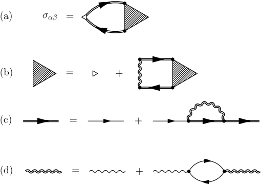
Figure 1: (a) Diagrammatic relationship (50) between the current Green function and the vertex. (b), (c) Equations for, respectively, the vertex function and the electron Green function in the mean-field approximation. (d) Coulomb interaction screening in the random-phase approximation.

Diagrammatic representation of the conductivity, shown in Fig. 1(a), allows its calculation in terms of the current vertex matrix $\Gamma_{\beta}$, which would be equal to $\sigma_{\beta}$ in the absence of interaction and disorder. To find it, we use the mean field approximation, where the excitonic ladder [Fig. 1(b)] for the vertex $\Gamma_{\beta}$ and the one-loop self-energy corrections [Fig. 1(c)] for the single-particle Green functions $G$ are taken into account. Using the interaction, which is statically screened in the random-phase approximation [Fig. 1(d)], greatly simplify the calculations. If we additionally neglect the mixing of different pairs of electron and hole Landau levels, appearing in the excitonic ladder (which was shown to be weak under typical conditions with using the screened interaction Sokolik1 ), the optical conductivity $\sigma_{\alpha\beta}(\omega)\equiv\sigma_{\alpha\beta}(0,\omega)$ is (see the details of calculations in Appendix C):

$$\sigma_{\alpha\beta}(\omega)=\frac{ie^{2}v_{\mathrm{F}}^{2}}{\omega}\sum_{n_{1}n_{2}}\frac{f_{n_{2}}-f_{n_{1}}}{\hbar\omega-\Omega_{n_{1}n_{2}}+i\delta}$$

$$\times\mathrm{Tr}\left[\Phi_{n_{1}n_{2}}(0)\sigma_{\alpha}\right]\mathrm{Tr}\left[\Phi^{+}_{n_{1}n_{2}}(0)\sigma_{\beta}\right].$$ (5)

Here $f_{n}$ is the occupation number ($0\leqslant f_{n}\leqslant 1$) of the $n$th Landau level, and the matrix $\Phi_{n_{1}n_{2}}(0)$, which is defined by (55) and (37), determines the selection rules $|n_{1}|=|n_{2}|\pm 1$ for each $n_{2}\rightarrow n_{1}$ transition. The resonant transition energy $\Omega_{n_{1}n_{2}}$, where $\sigma_{\alpha\beta}$ has a pole, consists of the difference between the bare Landau level energies $E_{n_{1}}-E_{n_{2}}$, the difference between electron self-energies $\Sigma_{n_{1}}-\Sigma_{n_{2}}$, and the excitonic correction $\Delta E_{n_{1},n_{2}}^{\mathrm{(exc)}}$ (see the similar formula in Shizuya2018 ):

$$\Omega_{n_{1}n_{2}}=E_{n_{1}}-E_{n_{2}}+\Sigma_{n_{1}}-\Sigma_{n_{2}}+\Delta E_{n_{1}n_{2}}^{\mathrm{(exc)}}.$$ (6)

In the mean field approximation, the self-energy

$$\Sigma_{n}=-\sum_{n^{\prime}}f_{n^{\prime}}\langle nn^{\prime}|V|n^{\prime}n\rangle,$$ (7)

as shown in Appendix B, is a sum of the exchange matrix elements

$$\langle nn^{\prime}|V|n^{\prime}n\rangle=2^{\delta_{n0}+\delta_{n^{\prime}0}-2}\frac{l_{H}^{2}}{2\pi}\int d\mathbf{q}\>V(q)$$

$$\times\left|s_{n}s_{n^{\prime}}\phi_{|n|-1,|n^{\prime}|-1}(\mathbf{a}_{\mathbf{q}})+\phi_{|n||n^{\prime}|}(\mathbf{a}_{\mathbf{q}})\right|^{2}$$ (8)

of the screened Coulomb interaction $V(q)$ between the $n$th and all filled $n^{\prime}$th Landau levels Iyengar ; Bychkov ; Faugeras1 , where the functions $\phi_{nk}$ are defined in (37), and $\mathbf{a}_{\mathbf{q}}\equiv-l_{H}^{2}[\mathbf{e}_{z}\times\mathbf{q}]$.

The excitonic correction

$$\Delta E_{n_{1}n_{2}}^{\mathrm{(exc)}}=-(f_{n_{2}}-f_{n_{1}})\langle n_{1}n_{2}|V|n_{1}n_{2}\rangle$$ (9)

is the direct interaction matrix element

$$\langle n_{1}n_{2}|V|n_{1}n_{2}\rangle=2^{\delta_{n_{1}0}+\delta_{n_{2}0}-2}\frac{l_{H}^{2}}{2\pi}\int d\mathbf{q}\>V(q)$$

$$\times\left\{\phi^{*}_{|n_{1}|-1,|n_{1}|-1}(\mathbf{a}_{\mathbf{q}})+\phi^{*}_{|n_{1}||n_{1}|}(\mathbf{a}_{\mathbf{q}})\right\}$$ (10)

$$\times\left\{\phi_{|n_{2}|-1,|n_{2}|-1}(\mathbf{a}_{\mathbf{q}})+\phi_{|n_{2}||n_{2}|}(\mathbf{a}_{\mathbf{q}})\right\}$$

with the minus sign, weighted with the difference of occupation numbers of the final and initial levels.

The dynamically screened interaction in the random-phase approximation is [see Fig. 1(d)]

$$V(q,i\omega)=\frac{v_{q}}{1-v_{q}\Pi(q,i\omega)},$$ (11)

where $v_{q}=2\pi e^{2}/\varepsilon q$ is the bare Coulomb interaction weakened by the surrounding medium with the dielectric constant $\varepsilon$, and

$$\Pi(q,i\omega)=g\sum_{nn^{\prime}}F_{nn^{\prime}}(q)\frac{f_{n}-f_{n^{\prime}}}{i\omega+E_{n}-E_{n^{\prime}}},$$ (12)

is the polarizability (or density response function) of noninteracting Dirac electrons Goerbig ; Roldan2 ; Lozovik ; Roldan3 ; Pyatkovskiy ; Gumbs . Here

$$F_{nn^{\prime}}(q)=2^{\delta_{n0}+\delta_{n^{\prime}0}-2}$$

$$\times\left|s_{n}s_{n^{\prime}}\phi_{|n|-1,|n^{\prime}|-1}(\mathbf{a}_{\mathbf{q}})+\phi_{|n||n^{\prime}|}(\mathbf{a}_{\mathbf{q}})\right|^{2}$$ (13)

is the form-factor of Landau level wave functions and $g=4$ is the degeneracy of electron states by valleys and spin. The statically screened interaction $V(q)$ is obtained from (11), (12) by taking $i\omega=0$.

In our model, there are three mechanisms leading to dependence of $\Omega_{n_{1}n_{2}}$ on the filling factor $\nu$ via the occupation numbers

$$f_{n}=\left\{\begin{array}[]{lll}0,&\mbox{if}&\nu\leq 4n-2,\\ (\nu-4n+2)/4,&\mbox{if}&4n-2<\nu<4n+2,\\ 1,&\mbox{if}&\nu\geq 4n+2,\end{array}\right.$$ (17)

i.e.: through exchange energies (7), excitonic corrections (9), and polarizability (12).

Note that the sum (7) over the filled Landau levels $n^{\prime}$ in the valence band diverges at $n^{\prime}\rightarrow-\infty$, so we impose the cutoff $n^{\prime}\geqslant-n_{\mathrm{c}}$ to obtain finite results. The physical reason of thus cutoff is a finite actual number of Landau levels in the valence band, which can be found from the total electron density: $n_{\mathrm{c}}=2\pi\hbar c/\sqrt{3}a^{2}eH\approx 39600/B[\mbox{T}]$, where $a\approx 2.46\,\mbox{\AA}$ Sokolik1 ; Sokolik2 .

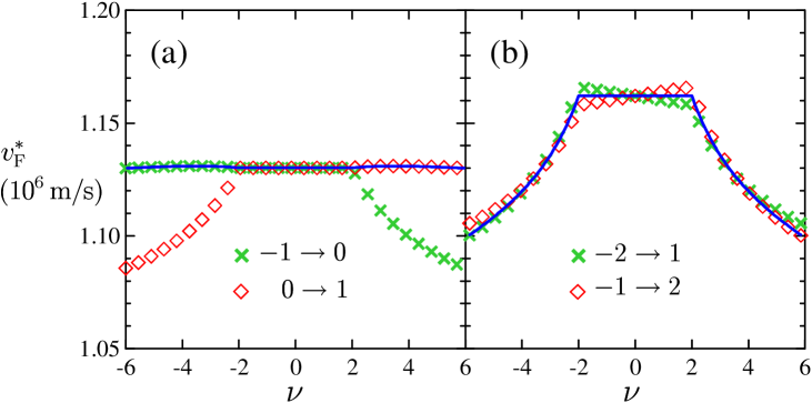
Figure 2: Renormalized Fermi velocities $v_{\mathrm{F}}^{*}$ for (a) the $T_{1}^{\pm}$ and (b) the $T_{2}^{\pm}$ transitions calculated with the screened interaction at $v_{\mathrm{F}}=0.85\times 10^{6}\,\mbox{m/s}$, $\varepsilon=3.27$, $B=8\,\mbox{T}$. Solid lines show the velocities found from the weighted transition energies (23).

III Electron-hole asymmetry and plateaus at $-2<\nu<2$

The selection rule $|n_{1}|=|n_{2}|\pm 1$ for the interband $n_{2}\rightarrow n_{1}$ transitions implies $n_{1},n_{2}=n+1,-n$ (the $\mathrm{T}_{n+1}^{+}$ transition) or $n_{1},n_{2}=n,-n-1$ (the $\mathrm{T}_{n+1}^{-}$ transition). In the idealized Dirac model without interactions, the energies of these transitions (2) are equal. However this is no longer the case when exchange self-energies are taken into account. Any nonzero doping $\nu\neq 0$ introduces an asymmetry between $\Omega_{n+1}^{+}$ and $\Omega_{n+1}^{-}$, at least, in the mean-field approximation. Looking at (6) and taking into account that $\langle n+1,-n|V|n+1,-n\rangle=\langle-n-1,n|V|-n-1,n\rangle$, we have:

$$\Omega_{n+1}^{+}-\Omega_{n+1}^{-}=\Sigma_{n+1}+\Sigma_{-n-1}-\Sigma_{n}-\Sigma_{-n}$$

$$+(f_{n}+f_{n+1}-f_{-n}-f_{-n-1})\langle n+1,-n|V|n+1,-n\rangle.$$ (18)

The electron-hole asymmetry in graphene, which is induced by the exchange interaction in the absence of magnetic field and is similar in scale to our case, was found in Kretinin .

The first line of (18) is a contribution of exchange self-energies to the asymmetry. Let us separate the occupation numbers $f_{n^{\prime}}=f_{n^{\prime}}^{(0)}+\Delta f_{n^{\prime}}$ on those of undoped graphene $f_{n^{\prime}}^{(0)}$ and the doping-induced part $\Delta f_{n^{\prime}}$, and define $\Sigma^{(0)}_{n}=-\sum_{n^{\prime}}f_{n^{\prime}}^{(0)}\langle nn^{\prime}|V|n^{\prime}n\rangle$. Using (8) and (43), and neglecting a difference of small matrix elements at $n^{\prime}\approx-n_{\mathrm{c}}$, we get $\Sigma^{(0)}_{n+1}+\Sigma^{(0)}_{-n-1}-\Sigma^{(0)}_{n}-\Sigma^{(0)}_{-n}=0$. Thus the exchange energy contribution to (18) arises only at nonzero doping $\nu\neq 0$.

The second line of (18) corresponding to excitonic effects is nonzero only when either $\pm n$th or $\pm(n+1)$th level is partially filled, i.e. at $4n-2<|\nu|<4n+6$. Since the polarizability (12) and hence the screened interaction $V(q)$ are even functions of $\nu$, both parts of (18) change sign at $\nu\rightarrow-\nu$, so

$$\Omega_{n+1}^{+}(\nu)=\Omega_{n+1}^{-}(-\nu).$$ (19)

This is illustrated in Fig. 2, where the typical calculated $v_{\mathrm{F}}^{*}$ are shown as functions of $\nu$.

The case of $n=0$ is the special one. The explicit structure of the wave functions (37) imply the following relationships connecting the matrix elements of direct and exchange interaction (valid even for non-Coulomb potentials):

$$\langle\pm 1,0|V|\pm 1,0\rangle+\langle\pm 1,0|V|0,\pm 1\rangle=\langle 00|V|00\rangle.$$ (20)

In result, the doping-induced changes of exchange and excitonic parts of (6) due to $f_{0}$ cancel each other at ${-2<\nu<2}$, when the 0th level is partially filled. Additionally, the polarizability (12) and hence $V(q)$ are also unchanged in this range of $\nu$, thus we expect plateaus in both $\Omega_{1}^{\pm}$:

$$\Omega_{1}^{+}(\nu)=\Omega_{1}^{-}(-\nu)=\mathrm{const}\quad\mbox{at}\quad-2<\nu<2,$$ (21)

as seen in Fig. 2(a). For $n\neq 0$ this is no longer the case, although variations of $\Omega_{n+1}^{\pm}(\nu)$ at $-2<\nu<2$ are typically very small [see Fig. 2(b)].

In experiments, $\Omega_{n+1}^{+}$ and $\Omega_{n+1}^{-}$ can be separated by observing cyclotron resonant absorption of light with opposite circular polarizations. Using linear polarization, one can observe a mixture of these transitions with relative intensities $I_{n+1}^{+}=f_{-n}-f_{n+1}$ and $I_{n+1}^{-}=f_{n}-f_{-n-1}$, equal to occupation number differences in final and initial states. Assuming that experimental apparatus does not resolve the individual lines $\Omega_{n+1}^{+}$ and $\Omega_{n+1}^{-}$, we will calculate the weighted transition energy

$$\langle\Omega_{n+1}\rangle=\frac{\Omega_{n+1}^{+}I_{n+1}^{+}+\Omega_{n+1}^{-}I_{n+1}^{-}}{I_{n+1}^{+}+I_{n+1}^{-}}$$ (22)

and compare it with the experiments in the next section. From the particle-hole symmetry relationship $f_{n}(-\nu)=1-f_{n}(\nu)$ we see that $\langle\Omega_{n+1}\rangle$ is even function of $\nu$. At $-2<\nu<2$, $\langle\Omega_{n+1}\rangle$ is linear (via $f_{0}$) and at the same time even function of $\nu$, so

$$\langle\Omega_{n+1}\rangle=\mathrm{const}\quad\mbox{at}\quad-2<\nu<2,$$ (23)

as seen in Figs. 2(a,b). Thus our model predicts plateaus in all weighted transition energies $\langle\Omega_{n+1}\rangle$ at $-2<\nu<2$. Similar conclusions about existence of the electron-hole asymmetry (18) and the conjugation property (19) were made in the recent theoretical work Shizuya2018 , which considers transition energies in the Hartree-Fock approximation.

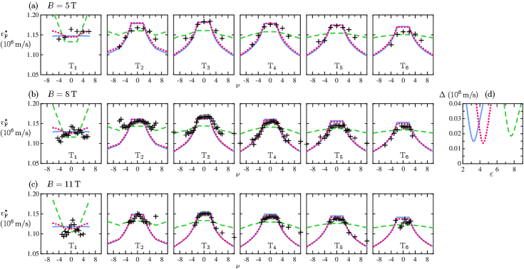
Figure 3: Renormalized Fermi velocities $v_{\mathrm{F}}^{*}$ at (a) $B=5$, (b) $8$, and (c) $11\,\mbox{T}$ for the set of the $T_{n+1}$ transitions ($-n\rightarrow n+1/-n-1\rightarrow n$), taken from the experiment Russell (crosses), and calculated theoretically in the Hartree-Fock approximation (dashed lines), with taking into account the interaction screening (solid lines) and with the self-consistent screening (dotted lines). The dielectric constants $\varepsilon$, used in each calculation, are listed in the first line of Table 1. Root mean square deviations (25) between the calculated and experimental $v_{\mathrm{F}}^{*}$ are also shown (d) as functions of $\varepsilon$ in the three approximations.

IV Calculation results

First we compare our calculations of the renormalized Fermi velocities

$$v_{\mathrm{F}}^{*}=\frac{\langle\Omega_{n+1}\rangle}{\sqrt{2Be\hbar/c}\left(\sqrt{n}+\sqrt{n+1}\right)}$$ (24)

with the data of Ref. Russell where $\Omega_{1}\ldots\Omega_{6}$ as functions of $\nu$ were measured at three magnetic fields $B=5,8,11\,\mbox{T}$. We fit the experimental points in three approximations:

1) Hartree-Fock approximation, where the unscreened Coulomb potential $v_{q}$ is used in all calculations.

2) Static random-phase approximation, where the potential $V(q)$ is screened (11) with using the polarizability of noninteracting electron gas in magnetic field.

3) Self-consistent screening approximation, where the polarizability is multiplied by $v_{\mathrm{F}}/v_{\mathrm{F}}^{*}$ to take into account weakening of the screening caused by many-body increase of the energy differences $E_{n^{\prime}}-E_{n}$ in denominators of (12). Similarly to our previous works Sokolik1 ; Sokolik2 , this semi-phenomenological model is aimed to achieve a self-consistency between many-body renormalizations of transition energies and screening. Using the iterative procedure, we take $v_{\mathrm{F}}^{*}$, obtained on each step, to renormalize the screening when calculating new $v_{\mathrm{F}}^{*}$ on the next step. About 5-6 iterations are usually sufficient to achieve a convergence.

Calculations in our approach depend only on two parameters: the bare Fermi velocity $v_{\mathrm{F}}$ and the dielectric constant of a surrounding medium $\varepsilon$. In principle, both $v_{\mathrm{F}}$ and $\varepsilon$ can be treated as fitting parameters. However variation of $v_{\mathrm{F}}$ in the range $(0.8\div 0.95)\times 10^{6}\,\mbox{m/s}$ allows to achieve almost equally good agreement with the experimental data at slightly different $\varepsilon$, so a simultaneous fitting of both parameters does not provide reliable results. Therefore we choose a specific value $v_{\mathrm{F}}=0.85\times 10^{6}\,\mbox{m/s}$, which was concluded to be the most suitable one based on theoretical fits of several experimental data on graphene both in presence Sokolik1 ; Yu and absence Elias ; YangPRL of magnetic field. After that, the optimal dielectric constant of the surrounding medium $\varepsilon$ is the only adjustable parameter in our model, and we find it by performing the least square fitting of the experimental points for all $n$ and $B$ simultaneously. Nevertheless it should be kept in mind that our fitting results can slightly change quantitatively with different choice of $v_{\mathrm{F}}$ (although qualitative conclusions will be the same), and it could be promising to implement a renormalization-group scheme for the Landau level data on graphene where all unobservable variables like $v_{\mathrm{F}}$ can be excluded from the model.

Table 1: Dielectric constants of surrounding medium $\varepsilon$, which provide the best least-square fittings of the experimental data from Refs. Russell ; Sonntag at $v_{\mathrm{F}}=0.85\times 10^{6}\,\mbox{m/s}$ in the three approximations for the interaction listed in Sec. IV.

	Unscreened	Screened	Self-consistent
Experiment	interaction	interaction	screening
Russell et al. Russell	7.72	3.27	4.36
Sonntag et al. Sonntag	5.50	1.05	2.55

The first line of Table 1 shows the optimal $\varepsilon$ used to fit the cyclotron resonance data of Ref. Russell where high-mobility graphene samples were encapsulated from both sides in hexagonal boron nitride monolayers and placed on an oxidized silicon. Fig. 3 shows the experimental points together with our calculations at these $\varepsilon$ in the three approximations described above. The calculation with the unscreened Coulomb interaction (Hartree-Fock approximation) demonstrates two significant drawbacks. First, the dielectric constant $\varepsilon\approx 7.72$ is unrealistically high, because in this approximation it should imitate the interaction screening by Dirac electrons in graphene in addition to the screening by an external medium. Second, the falloff of $v_{\mathrm{F}}^{*}$ at $|\nu|>2$ turns out to be insufficient, because the increase of the screening strength (and, consequently, suppression of the upward renormalization of the Fermi velocity) following the carrier density, is absent here. For the $T_{1}$ transitions, the calculated $v_{\mathrm{F}}^{*}$ even increases at $|\nu|>2$, in contradiction with the experiment, because the excitonic correction (9), which normally decrease $v_{\mathrm{F}}^{*}$, become suppressed due to partial filling of $1$th or $-1$th Landau level. The similar drawbacks of the Hartree-Fock approximations were mentioned in our previous works Sokolik1 ; Sokolik2 .

The screening allows us to achieve much better agreement with the experimental points at more realistic $\varepsilon\approx 3.27$, and the falloff of $v_{\mathrm{F}}^{*}$ at $|\nu|>2$ is reproduced very well. The iterative calculations with the self-consistent screening provide almost the same curves, but at somewhat higher $\varepsilon\approx 4.36$. This distinction arises because the higher $\varepsilon$ is needed to compensate the screening weakening caused by an upward renormalization of energy denominators in (12).

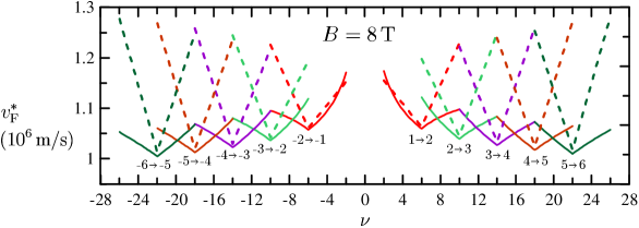
Figure 4: Renormalized Fermi velocities $v_{\mathrm{F}}^{*}$ for the intraband $n\rightarrow n+1$ and $-n-1\rightarrow-n$ transitions calculated at $B=8\,\mbox{T}$ in the Hartree-Fock approximation (dashed lines) and with taking into account the interaction screening (solid lines). The self-consistent iterative calculations are not shown because their results are close to those with the non-self-consistent screening. The dielectric constants $\varepsilon$ are taken from the first line of Table 1.

Our calculations with taking into account the screening are thus able to fit the data of Ref. Russell at three different $B$ and for six resonances $T_{n+1}$ simultaneously with the single adjustable parameter $\varepsilon$. We can explain both the decrease of $v_{\mathrm{F}}^{*}$ at $\nu=0$ as $B$ gets higher, the plateaus at $|\nu|<2$, and the rapid falloff of $v_{\mathrm{F}}^{*}$ at $|\nu|>2$, $n\geqslant 1$ due to increase of the screening strength. The exceptions are some inconsistencies of $v_{\mathrm{F}}^{*}$ at specific resonances ($\mathrm{T}_{2}$ and $\mathrm{T}_{6}$ at $B=5\,\mbox{T}$, $\mathrm{T}_{5}$ and $\mathrm{T}_{6}$ at $B=8\,\mbox{T}$) and the local maxima at $\nu=0$ for the $\mathrm{T}_{1}$ transitions. Moreover, the local minima of $v_{\mathrm{F}}^{*}$ for $\mathrm{T}_{2}$ at $\nu=\pm 4$, when the $1$th or $-1$th Landau level is half-filled, which occur only at $B=8\,\mbox{T}$ and are absent in other fields, are not predicted by our approach.

To characterize an accuracy of our fitting, we present in Fig. 3(d) the root mean square deviation

$$\Delta=\sqrt{\sum_{i=1}^{N}\frac{[(v_{\mathrm{F}}^{*})_{i}^{\mathrm{calc}}-(v_{\mathrm{F}}^{*})_{i}^{\mathrm{exp}}]^{2}}{N}}$$ (25)

of calculated renormalized Fermi velocities $(v_{\mathrm{F}}^{*})_{i}^{\mathrm{calc}}$ from $N$ experimental values $(v_{\mathrm{F}}^{*})_{i}^{\mathrm{exp}}$ (here it means for all fields and all resonances at once, 260 points in total). As functions of the fitting parameter $\varepsilon$, $\Delta$ reach rather sharp minima at optimal $\varepsilon$ in each approximation. The minimal $\Delta$ about $0.015\times 10^{6}\,\mbox{m/s}$ are comparable to the experimental uncertainties of $(v_{\mathrm{F}}^{*})_{i}^{\mathrm{exp}}$ Russell , so the fitting can be considered to be sufficiently accurate.

For completeness of the analysis, we can also consider the intraband transitions $n\rightarrow n+1$ and $-n-1\rightarrow-n$. Several examples calculated in the conditions of the experiment Russell are presented in Fig. 4. Each $n\rightarrow n+1$ ($-n-1\rightarrow-n$) transition exists in the range $4n-2<\nu<4n+6$ ($-4n-6<\nu<-4n+2$) of the filling factors, and the transition energies are minimal at $\nu=4n+2$ ($\nu=-4n-2$). These minima are caused by the excitonic correction (9), which is maximal when the initial Landau level is completely filled, and the final level is completely empty. We can also note that $v_{\mathrm{F}}^{*}$ again decreases with increasing the doping level due to enhancement of the screening, while the Hartree-Fock approximation misses this effect and greatly overestimates the variations of $v_{\mathrm{F}}^{*}$ vs. $\nu$. The electron-hole asymmetry for these transitions is negligible.

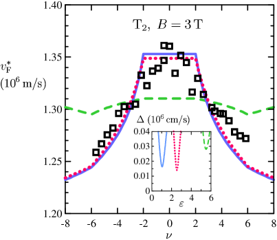
Figure 5: Renormalized Fermi velocity $v_{\mathrm{F}}^{*}$ for the $T_{2}$ transition ($-1\rightarrow 2/-2\rightarrow 1$) at $B=3\,\mbox{T}$, taken from the experiment Sonntag (squares) and calculated theoretically in the Hartree-Fock approximation (dashed lines), with taking into account the interaction screening (solid lines) and with the self-consistent screening (dotted lines). The dielectric constants $\varepsilon$, used in each approximation, are listed in the second line of Table 1. Inset shows root mean square deviations (25) between the calculated and experimental $v_{\mathrm{F}}^{*}$ as functions of $\varepsilon$ in the three approximations.

Another experiment we analyze is Ref. Sonntag where graphene is suspended $160\,\mbox{nm}$ above oxidized silicon, and the filling-factor dependence of the $\mathrm{T}_{2}$ transition energy was measured at $B=3\,\mbox{T}$ by observing its avoided crossing with the phonon energy in Raman spectrum. In Fig. 5 we plot the results of our calculations for this transition in the three approximations at optimal $\varepsilon$ listed in the second line of Table 1. We observe the same regularities as in the previous case. The Hartree-Fock approximations requires overestimated $\varepsilon$ and cannot explain the rapid falloff of $v_{\mathrm{F}}^{*}$ at $|\nu|>2$. At $|\nu|>6$ we see even slight increase of $v_{\mathrm{F}}^{*}$ due to suppression of the excitonic correction when the $2$nd or $-2$nd Landau level start to be partially filled. In contrast, with taking into account the screening we obtain the realistic $\varepsilon$ for graphene suspended above the oxidized silicon, and the falloff is well reproduced. Nevertheless, the experimental points demonstrate an additional maximum at $\nu=0$. This is not described by our approach, which predicts plateaus at $|\nu|<2$, as discussed in Sec. III.

The root mean square deviations (25), calculated for $31$ experimental points, are shown in the inset to Fig. 5 and demonstrate pronounced minima at the optimal $\varepsilon$. The minimal $\Delta$ about $0.015\times 10^{6}\,\mbox{m/s}$, achieved with the screened interaction, are comparable to the experimental uncertainties $(0.01\div 0.05)\times 10^{6}\,\mbox{m/s}$ Sonntag .

V Landau level broadening

One more experiment where the filling-factor dependent transition energy was measured is Ref. Henriksen . In this earlier work, graphene layer lied directly on an oxidized silicon substrate and carrier mobility was one-two orders of magnitude lower than in the aforementioned works Russell ; Sonntag due to charged impurities in the substrate. The $\mathrm{T}_{1}$ cyclotron resonance was studied at $B=18\,\mbox{T}$ and the unusual W-shaped form of the transition energy vs. $\nu$ was found with the local maximum at $\nu=0$ and two minima at integer Landau level fillings $\nu=\pm 2$.

To explain these results, we need to take into account disorder, because at mobilities of several thousands of $\mbox{cm}^{2}/\mbox{V}\cdot\mbox{s}$, reported in Henriksen , the disorder-induced Landau level widths $\sim 20\,\mbox{meV}$ become comparable with the energy scale $e^{2}/\varepsilon l_{H}$ of Coulomb interaction effects. The main mechanism of disorder effect on the transition energies is the following. Assume that Landau levels are broadened giving rise to Gaussian mini-bands in the density of states, as shown in Fig. 6. At partial filling of each level, its mini-band is partially filled, so the average energy of the filled (empty) electron states is lower (higher) than the band center where the unperturbed Landau level energy would be located. As a result, the average transition energy increases due to Landau level broadening in addition to interaction effects when either initial or final level is partially filled ($\nu\neq\pm 2$ in our case). The similar effect was discussed in Ando75 for a two-dimensional gas of massive electrons in the framework of self-consistent Born approximation.

To describe this effect, we assume the Gaussian spectral density $\rho_{n}(E)=(\sqrt{2\pi}\Gamma_{n})^{-1}\exp[-(E-E_{n})^{2}/2\Gamma_{n}^{2}]$ for each $n$th partially filled broadened level. Integrating it up to the Fermi level $\mu$ and assuming low temperature, we find the occupation number $f_{n}$, and, using (17), we get the relationship between $\nu$ and $\mu$: $\nu=4n+2\Phi([\mu-E_{n}]/\sqrt{2}\Gamma_{n})$, where $\Phi$ is the error function. The disorder-induced correction $\langle\Delta\Omega_{n}\rangle$ to the transition energy is a difference between the average energies (relative to the band centers) of empty states on a final Landau level and filled states on an initial level. It should be additionally weighted according to (23), when $-2<\nu<2$ and thus both transitions $\mathrm{T}_{1}^{\pm}$ are present, resulting in:

$$\langle\Delta\Omega_{n}\rangle=\left\{\begin{array}[]{rcl}\displaystyle\sqrt{\frac{2}{\pi}}\frac{\Gamma_{-1}e^{-\frac{(\mu-E_{-1})^{2}}{2\Gamma_{-1}^{2}}}}{3+\nu/2},&\mbox{if}&-6<\nu<-2,\\ \displaystyle\sqrt{\frac{2}{\pi}}\Gamma_{0}e^{-\frac{(\mu-E_{0})^{2}}{2\Gamma_{0}^{2}}},&\mbox{if}&-2<\nu<2,\\ \displaystyle\sqrt{\frac{2}{\pi}}\frac{\Gamma_{1}e^{-\frac{(\mu-E_{1})^{2}}{2\Gamma_{1}^{2}}}}{3-\nu/2},&\mbox{if}&\hphantom{-}2<\nu<6.\end{array}\right.$$ (29)

This dependence has a maximum at $\nu=0$ and minima at $\nu=\pm 2$ in accordance with the experiment Henriksen .

Another effect of the disorder is the presence of interlevel transitions when any $n$th Landau level is partially filled, which provide an extra contribution to the screening. In the simplest approximation, they lead to the polarizability of the Thomas-Fermi kind

$$\Pi^{\mathrm{TF}}_{n}(q)=-gF_{nn}(q)\rho_{n}(\mu),$$ (30)

which was used in Yang to study Landau level broadening in graphene.

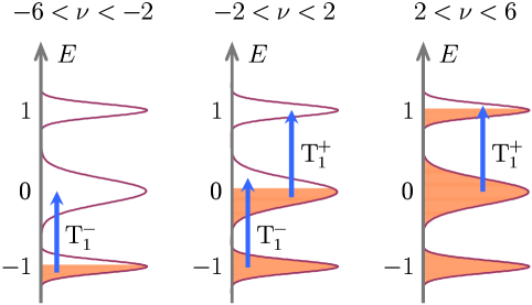
Figure 6: Broadened Landau levels $n=0,\pm 1$ (not in scale) and cyclotron transitions between them when these levels are partially filled.

We use the self-consistent Born approximation for a polarizability in magnetic field, which was originally developed in Ando71 ; Ando74 for a two-dimensional electron gas with short-range impurities. In our work, we assume the disorder to be long-ranged, because the main origin of disorder in graphene on a $\mathrm{SiO}_{2}$ substrate are long-range charged impurities DasSarma . Introducing the mean square $\langle U^{2}\rangle$ of the slowly varying disorder potential $U(\mathbf{r})$, we get the following polarizability of disordered graphene (see the similar formulas in Ando71 ; Ando74 obtained by summing an impurity ladder in a polarization loop):

$$\Pi^{\mathrm{D}}(q,i\omega)=g\sum_{nn^{\prime}}F_{nn^{\prime}}(q)$$

$$\times T\sum_{\epsilon}\frac{G^{\mathrm{D}}_{n^{\prime}}(i\epsilon+i\omega)G^{\mathrm{D}}_{n}(i\epsilon)}{1-\langle U^{2}\rangle G^{\mathrm{D}}_{n^{\prime}}(i\epsilon+i\omega)G^{\mathrm{D}}_{n}(i\epsilon)},$$ (31)

where $G^{\mathrm{D}}_{n}(i\epsilon)=\int dE\>\rho_{n}(E)/(i\omega-E+\mu)$ is the Green function of electron on the $n$th Landau level in the presence of disorder. Instead of a half-elliptic spectral density Yang , which is known to be an artefact of the self-consistent Born approximation MacDonald , we use, as above, the Gaussian function $\rho_{n}(E)$.

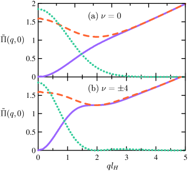
Figure 7: Dimensionless static polarizability of graphene in magnetic field $\tilde{\Pi}(q,0)=-(2\pi v_{\mathrm{F}}l_{H}/g)\Pi(q,0)$, where $l_{H}=\sqrt{\hbar c/eH}$, calculated (a) when the 0th Landau level is half-filled, $\nu=0$, (b) when the 1th or $-1$th level is half-filled, $\nu=\pm 4$. Solid lines: clean graphene (12), dashed lines: disordered graphene (33), dotted lines: the Thomas-Fermi approximation (30). Calculation parameters are $v_{\mathrm{F}}=0.85\times 10^{6}\,\mbox{m/s}$, $B=18\,\mbox{T}$, $\Gamma_{0}=\Gamma_{\pm 1}=20\,\mbox{meV}$.

Taking the static limit $i\omega\rightarrow 0$ and switching in (31) from the frequency summation to an integration along the branch cut at $\mathrm{Im}(i\epsilon)=0$, we get in the limit $T\rightarrow 0$:

$$\Pi^{\mathrm{D}}(q,0)=-\frac{g}{\pi}\sum_{nn^{\prime}}F_{nn^{\prime}}(q)$$

$$\times\int\limits_{-\infty}^{0}\mathrm{Im}\frac{G^{\mathrm{D}}_{n^{\prime}}(z+i\delta)G^{\mathrm{D}}_{n}(z+i\delta)}{1-\langle U^{2}\rangle G^{\mathrm{D}}_{n^{\prime}}(z+i\delta)G^{\mathrm{D}}_{n}(z+i\delta)}.$$ (32)

This polarizability consists of two physically distinct parts. The first one is the contribution of interlevel transitions with $n\neq n^{\prime}$. It does not differ too much from than in a clean system (12) if the widths of Landau levels $\Gamma_{n}$ are much smaller than interlevel separations. The second one is the contribution of intralayer transitions $n=n^{\prime}$ arising when the $n$th layer is partially filled. Taking the disorder strength to be equal to the Landau level width $\sqrt{\langle U^{2}\rangle}=\Gamma_{n}$, as follows from calculations of $G^{\mathrm{D}}$ with the long-range disorder, we get the static polarizability of disordered graphene:

$$\Pi^{\mathrm{D}}(q,0)\approx\Pi(q,0)-gF_{nn}(q)\int\limits_{-\infty}^{0}\mathrm{Im}\frac{[G^{\mathrm{D}}_{n}(z+i\delta)]^{2}}{1-\Gamma_{n}^{2}[G^{\mathrm{D}}_{n}(z+i\delta)]^{2}}$$ (33)

and use it in the following calculations.

Fig. 7 shows the examples of static polarizabilities calculated at half-fillings of 0th and $\pm 1$th Landau levels. In a clean graphene, $\Pi(q,0)\propto q^{2}$ at $q\rightarrow 0$ since the system becomes insulating in magnetic field, and the only source of the screening are gapped interlevel transitions. Disorder makes $\Pi^{\mathrm{D}}(q,0)$ nonzero at $q\rightarrow 0$ due to intralevel transitions. The Thomas-Fermi approximation, by taking into account only the latter, provides a wrong short-wavelength asymptotic of the polarizability $\Pi^{\mathrm{TF}}_{n}(q)$, which should tend to the polarizability of undoped graphene $\Pi(q,0)=-gq/16\hbar v_{\mathrm{F}}$ CastroNeto .

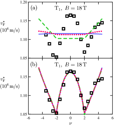
Figure 8: Renormalized Fermi velocity $v_{\mathrm{F}}^{*}$ for the $T_{1}$ transition ($0\rightarrow 1/-1\rightarrow 0$) at $B=18\,\mbox{T}$, taken from the experiment Henriksen (squares) and calculated theoretically for (a) clean and (b) disordered graphene. The calculations are carried out in the Hartree-Fock approximation (dashed lines), with taking into account the interaction screening (solid lines) and with the self-consistent screening (dotted lines). The dielectric constants $\varepsilon$ used in each calculation are listed in Table 2.

We calculated the renormalized Fermi velocity, corresponding to the weighted energy (23) of the $T_{1}$ transition with taking into account the correction (29) and the screening (33) in the disordered system. For comparison, we carried out the same calculations for the clean system, as did in the previous section. The results of the fitting of experimental points from Ref. Henriksen are shown in Fig. 8, and the calculation parameters are listed in Table 2.

Table 2: First two lines: dielectric constants of surrounding medium $\varepsilon$, which provide the best least-square fittings of the experimental data from Ref. Henriksen at $v_{\mathrm{F}}=0.85\times 10^{6}\,\mbox{m/s}$ in the three approximations for the interaction listed in Sec. IV for clean or disordered system. For disordered system, the widths of $0$th and $\pm 1$st Landau levels are also specified in the last two lines.

	Unscreened	Screened	Self-consistent
System	interaction	interaction	screening
Clean	7.26	2.82	3.85
Disordered	9.24	4.95	5.74
$\Gamma_{0}\,\mbox{(meV)}$	22	25	23
$\Gamma_{\pm 1}\,\mbox{(meV)}$	12	19	17

For the values of $\varepsilon$, we observe the same regularities as noted in the previous section. These values are close to those obtained in our earlier analysis Sokolik1 of cyclotron resonance data for graphene on $\mathrm{SiO}_{2}$. However the most drastic effects come from inclusion of disorder: while in the clean system $v_{\mathrm{F}}^{*}$ has the plateau at $|\nu|<2$ and remain the same (or slightly increases due to suppression of the excitonic correction) at $|\nu|>2$, in the disordered system it has the parabolic-like maximum at $\nu=0$ and the sharp minima at $\nu=\pm 2$, just as the experiment shows. The values of Landau level widths $\Gamma_{n}$ obtained via the fitting procedure ($15-25\,\mbox{meV}$) look realistic, since they are close to typical widths of spectral lines observed in the same experiment Henriksen and in other works on graphene on a $\mathrm{SiO}_{2}$ substrate Luican . The minimal value of the root mean square deviation (25) is about $0.009\times 10^{6}\,\mbox{m/s}$ in this case.

VI Conclusions

We present detailed calculations of the inter-Landau level cyclotron transition energies in graphene in strong magnetic fields taking into account Coulomb interaction between massless Dirac electrons. Calculating the optical conductivity and solving the vertex equation in the static random-phase approximation with the excitonic ladder, we found the many-body corrections to the transition energies coming from the self-energy and excitonic effects. We show that the cyclotron transition lines can be split in doped graphene for opposite circular polarizations because of the electron-hole asymmetry of exchange self-energies, although this splitting may be unobservable if these lines are sufficiently wide or either a linearly polarized or unpolarized light is used. By this reason, we calculate the weighted transition energy for both polarizations at once and convert it to the renormalized Fermi velocity $v_{\mathrm{F}}^{*}$ for each transition.

The dependence of $v_{\mathrm{F}}^{*}$ on the Landau level filling factor $\nu$ is analyzed. In the mean-field approximation, $v_{\mathrm{F}}^{*}(\nu)$ has a plateau at $-2<\nu<2$ due to a partial cancelation of the self-energy and excitonic effects and rapidly decreases at $|\nu|>2$ due to enhancement of the screening. Our calculations, carried out with the bare Fermi velocity $v_{\mathrm{F}}=0.85\times 10^{6}\,\mbox{m/s}$ and with the dielectric constant of surroundings $\varepsilon$, treated as an adjustable parameter, showed good agreement with two recent experiments Russell ; Sonntag on high-mobility graphene samples, when the screening by graphene electrons is taken into account. The obtained phenomenological $\varepsilon$ describe the external dielectric screening not only by an underlaying substrate, but also by adjacent hexagonal boron nitride layers. The Hartree-Fock approximation, which neglects the density-dependent screening by graphene electrons, fails to explain the observed rapid decrease of $v_{\mathrm{F}}^{*}$ at $|\nu|>2$.

Our calculations for the intraband transitions $n\rightarrow n+1$ and $-n-1\rightarrow-n$ predict the V-like dependence $v_{\mathrm{F}}^{*}(\nu)$ with the minima at, respectively, $\nu=4n+2$ and $\nu=-4n-2$ caused by the excitonic effects. Existence of these minima can be verified experimentally, although an accurate detection of the interband transition lines can be challenging (but possible Sadowski1 ) due to their much lower energies: even for the the highest magnetic fields 20-30 T these energies are below 100 meV.

We also describe the data of the earlier cyclotron resonance experiment Henriksen with graphene sample on $\mathrm{SiO}_{2}$, where carrier mobility is much lower. In this case we take into account long-range disorder, which broadens Landau levels and thus shifts the resonant energy upward when initial or final level is partially filled, and induces the interlevel transitions contributing to the screening. Assuming the Gaussian spectral density for the $0$th and $\pm 1$th broadened Landau levels, we achieved good agreement with the experiment and explained the main features of the $v_{\mathrm{F}}^{*}(\nu)$ dependence: the parabolic-like maximum at $\nu=0$ and the sharp minima at $\nu=\pm 2$.

As shown, the combined action of exchange interaction, excitonic effects, interaction screening and disorder should be taken into account when considering graphene in strong magnetic field. Our approach takes into consideration these factors and thus allowed us to explain main features of the filling-factor dependent experimental data Russell ; Sonntag ; Henriksen , which would be hardly possible within the Hartree-Fock approximation Iyengar ; Bychkov ; Barlas ; Roldan1 ; Shizuya1 ; Shizuya2 ; Faugeras1 ; Chizhova ; Shizuya4 ; Shizuya2018 where the screening and Landau level broadening are neglected. However, some issues remain to be clarified. In particular, the mean-field approach does not describe the $\Lambda$-shaped maxima of $v_{\mathrm{F}}^{*}$ at $\nu=0$ observed in Russell ; Sonntag for $\mathrm{T}_{1}$ transitions, the minima at $\nu=\pm 4$ observed for $\mathrm{T}_{2}$ at $B=8\,\mbox{T}$ in Russell , and a possible splitting of the $\mathrm{T}_{1}$ transition line observed in Russell . All these features go beyond the mean-field theory for massless Dirac electrons and can be attributed to some unaccounted role of disorder, finite size effects, Moire superlattice potential from adjacent boron nitride layers ChenNComm , Landau level splitting Goerbig ; Song or electron dynamics on a partially filled level Basko . Note that assumption of a substrate-induced band gap allowed to explain some features of the experimental data of Russell in the recent work Shizuya2018 , so a further analysis in this direction with considering possible symmetry breakings and gap formation in a system of Dirac electrons together with the interaction, screening and disorder seems to be promising.

Appendix A Electron wave functions

Similarly to Pyatkovskiy ; Roldan3 ; Lozovik ; Goerbig , we describe single-particle states of massless electrons in magnetic field $\mathbf{H}$ using the symmetric gauge $\mathbf{A}=\frac{1}{2}\left[\mathbf{H}\times\mathbf{r}\right]$. In the absence of a valley splitting or intervalley transitions, it is sufficient to consider the electrons only in the $\mathbf{K}$ valley, where the Dirac Hamiltonian is

$$H=v_{\mathrm{F}}\left(\mathbf{p}-\frac{e}{c}\mathbf{A}\right)\cdot\boldsymbol{\sigma}=\frac{\hbar v_{\mathrm{F}}\sqrt{2}}{l_{H}}\left(\begin{array}[]{cc}0&a\\ a^{+}&0\end{array}\right).$$ (36)

Here $l_{H}=\sqrt{\hbar c/|e|H}$ is the magnetic length (we assume $e<0$ in this section), $a=l_{H}p_{-}/\hbar-ir_{-}/2l_{H}$ and $a^{+}=l_{H}p_{+}/\hbar+ir_{+}/2l_{H}$ are, respectively, lowering and raising operators obeying the commutation relation $[a,a^{+}]=1$, and $p_{\pm}=(p_{x}\pm ip_{y})/\sqrt{2}$, $r_{\pm}=(x\pm iy)/\sqrt{2}$.

Introducing the complementary set of ladder operators Goerbig $b=l_{H}p_{+}/\hbar-ir_{+}/2l_{H}$, $b^{+}=l_{H}p_{-}/\hbar+ir_{-}/2l_{H}$, which obey $[b,b^{+}]=1$ and commute with $a$, $a^{+}$, we can construct the states of a two-dimensional oscillator $|\phi_{nk}\rangle=(a^{+})^{n}(b^{+})^{k}|\phi_{00}\rangle/\sqrt{n!k!}$ with the wave functions in polar coordinates:

$$\phi_{nk}(r,\varphi)=\frac{i^{|n-k|}}{\sqrt{2\pi}l_{H}}\sqrt{\frac{\min(n,k)!}{\max(n,k)!}}\>e^{-r^{2}/4l_{H}^{2}}\left(\frac{r}{\sqrt{2}l_{H}}\right)^{|n-k|}e^{i(n-k)\varphi}L_{\min(n,k)}^{|n-k|}\left(\frac{r^{2}}{2l_{H}^{2}}\right),$$ (37)

where $L_{n}^{m}(x)$ are the associated Laguerre polynomials. The eigenfunctions of the Hamiltonian (36) are Gumbs ; Roldan2 ; Roldan3 ; Barlas ; Iyengar ; Roldan1 ; Goerbig ; Bychkov ; Lozovik

$$\psi_{nk}=(\sqrt{2})^{\delta_{n0}-1}\left(\begin{array}[]{r}s_{n}\phi_{|n|-1,k}\\ \phi_{|n|,k}\end{array}\right),$$ (40)

and eigenvalues are (1). Here $n=0,\pm 1,\pm 2,\ldots$ is the Landau level number, $k=0,1,2,\ldots$ is the guiding center index responsible for Landau levels degeneracy, $s_{n}\equiv\mathrm{sign}\,(n)$, and we assume that $\phi_{nk}=0$ if $n$ or $k$ is negative.

The bare electron Green function in the Matsubara representation $G(\mathbf{r},\mathbf{r}^{\prime},\tau)=-\langle T_{\tau}\Psi(\mathbf{r},\tau)\Psi^{+}(\mathbf{r}^{\prime},0)\rangle$ can be constructed from (40):

$$G_{0}(\mathbf{r},\mathbf{r}^{\prime},i\epsilon)=\sum_{nk}\frac{\psi_{nk}(\mathbf{r})\psi_{nk}^{+}(\mathbf{r}^{\prime})}{i\epsilon-E_{n}+\mu},$$ (41)

where $\mu$ is the chemical potential; note $G_{0}$ is the $(2\times 2)$ matrix in the sublattice space.

Using the table integral Eq. 2.20.16.10 from Prudnikov , we can present (37) in Cartesian coordinates as

$$\phi_{nk}(x,y)=\frac{i^{n-k}}{\sqrt{2\pi}}\int_{-\infty}^{+\infty}dt\>e^{ity}\varphi_{n}\left(l_{H}t+x/2l_{H}\right)\varphi_{k}\left(l_{H}t-x/2l_{H}\right),$$ (42)

where $\varphi_{n}(x)=e^{-x^{2}/2}H_{n}(x)/\sqrt{2^{n}n!\sqrt{\pi}}$ are the dimensionless eigenfunctions of quantum one-dimensional harmonic oscillator, $H_{n}(x)$ are Hermite polynomials. Then, using (42), and orthonormality and completeness of the basis $\{\varphi_{n}(x)\}$, a lot of useful transformation rules for $\phi_{nk}$ can be obtained, for example, the summation formula

$$\sum_{k=0}^{\infty}\phi_{n_{1}k}(\mathbf{r_{1}})\phi^{*}_{n_{2}k}(\mathbf{r}_{2})=\frac{e^{i(\mathbf{r}_{1}\mathbf{r}_{2}\mathbf{e}_{z})/2l_{H}^{2}}}{\sqrt{2\pi}l_{H}}\,\phi_{n_{1}n_{2}}(\mathbf{r}_{1}-\mathbf{r}_{2})$$ (43)

and the form-factor of Landau level wave functions (see also Pyatkovskiy )

$$\int d\mathbf{r}\>e^{i\mathbf{q}\mathbf{r}}\phi^{*}_{n_{1}n_{2}}(\mathbf{r})\phi_{n_{3}n_{4}}(\mathbf{r})=2\pi l_{H}^{2}\phi^{*}_{n_{1}n_{3}}(\mathbf{a}_{\mathbf{q}})\phi_{n_{2}n_{4}}(\mathbf{a}_{\mathbf{q}}),\qquad\mathbf{a}_{\mathbf{q}}\equiv-l_{H}^{2}[\mathbf{e}_{z}\times\mathbf{q}].$$ (44)

Appendix B Exchange self-energies

Exchange self-energy acquired by an electron in the state $\psi_{nk}$ is given by the usual Fock expression

$$\Sigma_{nk}^{\mathrm{exch}}=-\sum_{n^{\prime}k^{\prime}}f_{n^{\prime}k^{\prime}}\int d\mathbf{r}_{1}d\mathbf{r}_{2}\>v(\mathbf{r}_{1}-\mathbf{r}_{2})\psi^{+}_{nk}(\mathbf{r}_{1})\psi_{n^{\prime}k^{\prime}}(\mathbf{r}_{1})\psi^{+}_{n^{\prime}k^{\prime}}(\mathbf{r}_{2})\psi_{nk}(\mathbf{r}_{2}).$$ (45)

After the Fourier transform of the Coulomb interaction $v(\mathbf{r})=(2\pi)^{-2}\int d\mathbf{q}\>v_{q}e^{i\mathbf{qr}}$ and using (43)–(44), we get

$$\Sigma_{nk}^{\mathrm{exch}}=-\sum_{n^{\prime}}f_{n^{\prime}}\langle nn^{\prime}|v|n^{\prime}n\rangle$$ (46)

with the exchange matrix elements of Coulomb interaction defined as

$$\langle nn^{\prime}|v|n^{\prime}n\rangle=2^{\delta_{n0}+\delta_{n^{\prime}0}-2}\frac{l_{H}^{2}}{2\pi}\int d\mathbf{q}\>v_{q}\left|s_{n}s_{n^{\prime}}\phi_{|n|-1,|n^{\prime}|-1}(\mathbf{a}_{\mathbf{q}})+\phi_{|n||n^{\prime}|}(\mathbf{a}_{\mathbf{q}})\right|^{2}.$$ (47)

We assumed that the occupation numbers do not depend on $k^{\prime}$, $f_{n^{\prime}k^{\prime}}\equiv f_{n^{\prime}}$, and the resulting $\Sigma_{nk}^{\mathrm{exch}}$ turns out to be also independent on $k$, so the Landau level degeneracy is preserved. By replacing $v_{q}$ with the statically screened interaction $V(q)$, as depicted in Fig. 1(c), we get the screened exchange energy (7)–(8), and the bare electron Green function (41) becomes “dressed” with the interaction and turns into

$$G(\mathbf{r},\mathbf{r}^{\prime},i\epsilon)=\sum_{nk}\frac{\psi_{nk}(\mathbf{r})\psi_{nk}^{+}(\mathbf{r}^{\prime})}{i\epsilon-E_{n}-\Sigma_{n}+\mu}.$$ (48)

Appendix C Vertex equation

Introducing the Green function for currents $G^{j}_{\alpha\beta}(\mathbf{r},\mathbf{r}^{\prime},\tau)=-\langle T_{\tau}\Psi^{+}(\mathbf{r},\tau)\sigma_{\alpha}\Psi(\mathbf{r},\tau)\Psi^{+}(\mathbf{r}^{\prime},0)\sigma_{\beta}\Psi(\mathbf{r}^{\prime},0)\rangle$, we can write the conductivity (4) as

$$\sigma_{\alpha\beta}(\mathbf{q},\omega)=\frac{ie^{2}v_{\mathrm{F}}^{2}}{\hbar\omega S}\int d\mathbf{r}d\mathbf{r}^{\prime}\>e^{-i\mathbf{q}(\mathbf{r}-\mathbf{r}^{\prime})}G^{j}_{\alpha\beta}(\mathbf{r},\mathbf{r}^{\prime},\hbar\omega+i\delta),$$ (49)

where $G^{j}_{\alpha\beta}$ can be calculated, as shown in Fig. 1(a), from the $(2\times 2)$ vertex matrix:

$$G^{j}_{\alpha\beta}(\mathbf{r},\mathbf{r}^{\prime},i\omega)=T\sum_{\varepsilon}\int d\mathbf{r}_{1}d\mathbf{r}_{2}\>\mathrm{Tr}\left[\sigma_{\alpha}G(\mathbf{r},\mathbf{r}_{1},i\epsilon+i\omega)\Gamma_{\beta}(\mathbf{r}_{1},\mathbf{r}_{2},\mathbf{r}^{\prime},i\epsilon,i\omega)G(\mathbf{r}_{2},\mathbf{r},i\epsilon)\right].$$ (50)

Here the sum is taken over the fermionic Matsubara frequencies $\epsilon=\pi T(2n+1)$.

The vertex equation in the mean-field (or ladder) approximation, depicted in Fig. 1(b), is written analytically as

$$\Gamma_{\beta}(\mathbf{r}_{1},\mathbf{r}_{2},\mathbf{r}^{\prime},i\epsilon,i\omega)=\delta(\mathbf{r}_{1}-\mathbf{r}^{\prime})\delta(\mathbf{r}_{2}-\mathbf{r}^{\prime})\sigma_{\beta}-T\sum_{\epsilon^{\prime}}\int d\mathbf{r}_{1}^{\prime}d\mathbf{r}_{2}^{\prime}\>V(\mathbf{r}_{1}-\mathbf{r}_{2},i\epsilon-i\epsilon^{\prime})$$

$$\times G(\mathbf{r}_{1},\mathbf{r}_{1}^{\prime},i\epsilon^{\prime}+i\omega)\Gamma_{\beta}(\mathbf{r}_{1}^{\prime},\mathbf{r}_{2}^{\prime},\mathbf{r}^{\prime},i\epsilon^{\prime},i\omega)G(\mathbf{r}_{2}^{\prime},\mathbf{r}_{2},i\epsilon^{\prime}).$$ (51)

To solve it, we can use the basis of magnetoexcitonic states of Dirac electrons in the symmetric gauge, which were described earlier in Lozovik in slightly different notation:

$$\Psi_{\mathbf{P}n_{1}n_{2}}(\mathbf{r}_{1},\mathbf{r}_{2})=\frac{1}{2\pi}e^{i\mathbf{P}(\mathbf{r}_{1}+\mathbf{r}_{2})/2+i(\mathbf{r}_{1}\mathbf{r}_{2}\mathbf{e}_{z})/2l_{H}^{2}}\Phi_{n_{1}n_{2}}(\mathbf{r}_{1}-\mathbf{r}_{2}-\mathbf{a}_{\mathbf{P}}).$$ (52)

Here $\mathbf{P}$ is the conserved magnetic momentum of the electron-hole pair and

$$\Phi_{n_{1}n_{2}}(\mathbf{r})=\sqrt{2}^{\delta_{n_{1}0}+\delta_{n_{2}0}-2}\left(\begin{array}[]{cc}s_{n_{1}}s_{n_{2}}\phi_{|n_{1}|-1,|n_{2}|-1}(\mathbf{r})&s_{n_{1}}\phi_{|n_{1}|-1,|n_{2}|}(\mathbf{r})\\ s_{n_{2}}\phi_{|n_{1}|,|n_{2}|-1}(\mathbf{r})&\phi_{|n_{1}|,|n_{2}|}(\mathbf{r})\end{array}\right)$$ (55)

is the matrix wave function of relative motion of electron and hole written in the basis of their sublattices $A$, $B$. Using (42), the unitary transformations between the magnetoexcitonic states and the states (40) of individual electron and hole can be derived:

$$\psi_{n_{1}k_{1}}(\mathbf{r}_{1})\psi^{+}_{n_{2}k_{2}}(\mathbf{r}_{2})=l_{H}^{2}\!\!\int d\mathbf{P}\>\phi_{k_{1}k_{2}}^{*}(\mathbf{a}_{\mathbf{P}})\Psi_{\mathbf{P}n_{1}n_{2}}(\mathbf{r}_{1},\mathbf{r}_{2}),\quad\Psi_{\mathbf{P}n_{1}n_{2}}(\mathbf{r}_{1},\mathbf{r}_{2})=l_{H}^{2}\!\!\sum_{k_{1}k_{2}}\phi_{k_{1}k_{2}}(\mathbf{a}_{\mathbf{P}})\psi_{n_{1}k_{1}}(\mathbf{r}_{1})\psi^{+}_{n_{2}k_{2}}(\mathbf{r}_{2}).$$ (56)

Projecting the vertex matrix $\Gamma_{\beta}$ on the magnetoexcitonic states

$$\Gamma_{\beta,\mathbf{P}n_{1}n_{2}}(\mathbf{r}^{\prime},i\epsilon,i\omega)=\int d\mathbf{r}_{1}d\mathbf{r}_{2}\>\mathrm{Tr}\left[\Psi^{+}_{\mathbf{P}n_{1}n_{2}}(\mathbf{r}_{1},\mathbf{r}_{2})\Gamma_{\beta}(\mathbf{r}_{1},\mathbf{r}_{2},\mathbf{r}^{\prime},i\epsilon,i\omega)\right]$$ (57)

and using (48), (56), we get (51) in the electron-hole pair (or magnetoexcitonic) representation:

$$\Gamma_{\beta,\mathbf{P}n_{1}n_{2}}(\mathbf{r}^{\prime},i\epsilon,i\omega)=\Gamma^{(0)}_{\beta,\mathbf{P}n_{1}n_{2}}(\mathbf{r}^{\prime})-T\sum_{\epsilon^{\prime}n_{1}^{\prime}n_{2}^{\prime}}\int d\mathbf{P}^{\prime}\>\frac{\langle\Psi_{\mathbf{P}n_{1}n_{2}}|V(i\epsilon-i\epsilon^{\prime})|\Psi_{\mathbf{P}^{\prime}n_{1}^{\prime}n_{2}^{\prime}}\rangle\Gamma_{\beta,\mathbf{P}^{\prime}n_{1}^{\prime}n_{2}^{\prime}}(\mathbf{r}^{\prime},i\epsilon^{\prime},i\omega)}{(i\epsilon^{\prime}+i\omega-E_{n_{1}^{\prime}}-\Sigma_{n_{1}^{\prime}}+\mu)(i\epsilon^{\prime}-E_{n_{2}^{\prime}}-\Sigma_{n_{2}^{\prime}}+\mu)}.$$ (58)

Here the bare vertex is $\Gamma^{(0)}_{\beta,\mathbf{P}n_{1}n_{2}}(\mathbf{r}^{\prime})=(e^{-i\mathbf{Pr}^{\prime}}/2\pi)\,\mathrm{Tr}\left[\Phi^{+}_{n_{1}n_{2}}(\mathbf{a}_{\mathbf{P}})\sigma_{\beta}\right]$.

To solve Eq. (58), we use the static approximation $V(\mathbf{r},i\epsilon-i\epsilon^{\prime})=V(\mathbf{r})$ and neglect the mixing of different electron-hole pairs in the ladder diagrams, assuming $n_{1}^{\prime}=n_{1}$, $n_{2}^{\prime}=n_{2}$. Therefore the vertex matrix turns out to be independent on a relative energy of electron and hole $\epsilon$:

$$\Gamma_{\beta,\mathbf{P}n_{1}n_{2}}(\mathbf{r}^{\prime},i\omega)=\frac{e^{-i\mathbf{Pr}^{\prime}}}{2\pi}\,\mathrm{Tr}\left[\Phi^{+}_{n_{1}n_{2}}(\mathbf{a}_{\mathbf{P}})\sigma_{\beta}\right]\left\{1+\langle n_{1}n_{2}|V_{\mathbf{P}}|n_{1}n_{2}\rangle\frac{f_{n_{2}}-f_{n_{1}}}{i\omega+E_{n_{2}}+\Sigma_{n_{2}}-E_{n_{1}}-\Sigma_{n_{1}}}\right\}^{-1}.$$ (59)

The average interaction energies of magnetoexcitons are $\langle n_{1}n_{2}|V_{\mathbf{P}}|n_{1}n_{2}\rangle=\int d\mathbf{r}\>V(\mathbf{r}-\mathbf{a}_{\mathbf{P}})\mathrm{Tr}\left[\Phi^{+}_{n_{1}n_{2}}(\mathbf{r})\Phi_{n_{1}n_{2}}(\mathbf{r})\right]$, their counterparts in usual 2D electron gas were extensively studied earlier Butov . Making the Fourier transform $V(\mathbf{r})=(2\pi)^{-2}\int d\mathbf{q}\>V(q)e^{i\mathbf{qr}}$ and using (44), we obtain

$$\langle n_{1}n_{2}|V_{\mathbf{P}}|n_{1}n_{2}\rangle=\frac{l_{H}^{2}}{2\pi}\int d\mathbf{q}\>V(q)e^{-i\mathbf{qa}_{\mathbf{P}}}\mathrm{Tr}\left[\Phi^{+}_{n_{1}n_{1}}(\mathbf{a}_{\mathbf{q}})\right]\mathrm{Tr}\left[\Phi_{n_{2}n_{2}}(\mathbf{a}_{\mathbf{q}})\right].$$ (60)

The Green function for currents (50) can by found using (48), (52), (56), (57), and (59):

$$G_{\alpha\beta}^{j}(\mathbf{r},\mathbf{r}^{\prime},i\omega)=\sum_{n_{1}n_{2}}\int\frac{d\mathbf{P}}{(2\pi)^{2}}\,e^{i\mathbf{P}(\mathbf{r}-\mathbf{r}^{\prime})}\frac{\mathrm{Tr}\left[\Phi_{n_{1}n_{2}}(\mathbf{a}_{\mathbf{P}})\sigma_{\alpha}\right]\mathrm{Tr}\left[\Phi^{+}_{n_{1}n_{2}}(\mathbf{a}_{\mathbf{P}})\sigma_{\beta}\right](f_{n_{2}}-f_{n_{1}})}{i\omega+E_{n_{2}}+\Sigma_{n_{2}}-E_{n_{1}}-\Sigma_{n_{1}}+(f_{n_{2}}-f_{n_{1}})\langle n_{1}n_{2}|V_{\mathbf{P}}|n_{1}n_{2}\rangle}.$$ (61)

Substituting it in (49) and taking $\mathbf{P}=0$ for optical transitions in (60), we finally obtain (5)–(10).

References

• (1) A. H. Castro Neto, F. Guinea, N. M. R. Peres, K. S. Novoselov, and A. K. Geim, The electronic properties of graphene, Rev. Mod. Phys. 81, 109 (2009).
• (2) K. S. Novoselov, A. K. Geim, S. V. Morozov, D. Jiang, M. I. Katsnelson, I. V. Grigorieva, S. V. Dubonos, and A. A. Firsov, Two-dimensional gas of massless Dirac fermions in graphene, Nature 438, 197 (2005).
• (3) V. N. Kotov, B. Uchoa, V. M. Pereira, F. Guinea, and A. H. Castro Neto, Electron-Electron Interactions in Graphene: Current Status and Perspectives, Rev. Mod. Phys. 84, 1067 (2012).
• (4) M. O. Goerbig, Electronic properties of graphene in a strong magnetic field, Rev. Mod. Phys. 83, 1193 (2011).
• (5) L.-J. Yin, K.-K. Bai, W. Wang, S.-Y. Li, Y. Zhang, and L. He, Landau quantization of Dirac fermions in graphene and its multilayers, Front. Phys. 12, 127208 (2017).
• (6) M.L. Sadowski, G. Martinez, M. Potemski, C. Bergert, and W.A. De Heer, Magneto-spectroscopy of epitaxial graphene, Int. J. Mod. Phys. B 21, 1145 (2007).
• (7) M. Orlita and M. Potemski, Dirac electronic states in graphene systems: optical spectroscopy studies, Semicond. Sci. Technol. 25, 063001 (2010).
• (8) D. N. Basov, M. M. Fogler, A. Lanzara, F. Wang, and Y. Zhang, Colloquium: Graphene spectroscopy, Rev. Mod. Phys. 86, 959 (2014).
• (9) Z. Jiang, E. A. Henriksen, L. C. Tung, Y.-J. Wang, M. E. Schwartz, M. Y. Han, P. Kim, and H. L. Stormer, Infrared spectroscopy of Landau levels of graphene, Phys. Rev. Lett. 98, 197403 (2007).
• (10) Z. Jiang, E. A. Henriksen, P. Cadden-Zimansky, L.-C. Tung, Y.-J. Wang, P. Kim, and H. L. Stormer, Cyclotron resonance near the charge neutrality point of graphene, AIP Conf. Proc. 1399, 773 (2011).
• (11) E. A. Henriksen, P. Cadden-Zimansky, Z. Jiang, Z. Q. Li, L.-C. Tung, M. E. Schwartz, M. Takita, Y.-J. Wang, P. Kim, and H. L. Stormer, Interaction-induced shift of the cyclotron resonance of graphene using infrared spectroscopy, Phys. Rev. Lett. 104, 067404 (2010).
• (12) B. J. Russell, B. Zhou, T. Taniguchi, K. Watanabe, and E. A. Henriksen, Many-Particle Effects in the Cyclotron Resonance of Encapsulated Monolayer Graphene, Phys. Rev. Lett. 120, 047401 (2018).
• (13) J. Sonntag, S. Reichardt, L. Wirtz, B. Beschoten, M. I. Katsnelson, F. Libisch, C. Stampfer, Impact of Many-Body Effects on Landau Levels in Graphene, Phys. Rev. Lett. 120, 187701 (2018).
• (14) S. Berciaud, M. Potemski, and C. Faugeras, Probing electronic excitations in mono- to pentalayer graphene by micro magneto-Raman spectroscopy, Nano Lett. 14, 4548 (2014).
• (15) C. Faugeras, S. Berciaud, P. Leszczynski, Y. Henni, K. Nogajewski, M. Orlita, T. Taniguchi, K. Watanabe, C. Forsythe, P. Kim, R. Jalil, A. K. Geim, D. M. Basko, and M. Potemski, Landau level spectroscopy of electron-electron interactions in graphene, Phys. Rev. Lett. 114, 126804 (2015).
• (16) C. Faugeras, M. Orlita, and M. Potemski, Raman scattering of graphene-based systems in high magnetic fields, J. Raman Spectrosc. 49, 146 (2018).
• (17) W. Kohn, Cycloron resonance and de Haas-van Alphen oscillations of an interacting electron gas, Phys. Rev. 123, 1242 (1961).
• (18) A. Iyengar, J. Wang, H. A. Fertig, and L. Brey, Excitations from filled Landau levels in graphene, Phys. Rev. B 75, 125430 (2007).
• (19) Yu. A. Bychkov and G. Martinez, Magnetoplasmon excitations in graphene for filling factors $\nu\leqslant 6$, Phys. Rev. B 77, 125417 (2008).
• (20) R. Roldán, J.-N. Fuchs, and M. O. Goerbig, Spin-flip excitations, spin waves, and magnetoexcitons in graphene Landau levels at integer filling factors, Phys. Rev. B 82, 205418 (2010).
• (21) Y. Barlas, W.-C. Lee, K. Nomura, and A. H. MacDonald, Renormalized Landau levels and particle-hole symmetry in graphene, Int. J. Mod. Phys. B 23, 2634 (2009).
• (22) K. Shizuya, Many-body corrections to cyclotron resonance in monolayer and bilayer graphene, Phys. Rev. B 81, 075407 (2010).
• (23) K. Shizuya, Many-body corrections to cyclotron resonance in graphene, J. Phys.: Conf. Ser. 334, 012046 (2011).
• (24) L. A. Chizhova, J. Burgdorfer, and F. Libisch, Magneto-optical response of graphene: Probing substrate interactions, Phys. Rev. B 92, 125411 (2015).
• (25) K. Shizuya, Many-body effects on Landau-level spectra and cyclotron resonance in graphene, Phys. Rev. B 98, 115419 (2018).
• (26) E. V. Gorbar, V. P. Gusynin, V. A. Miransky, and I. A. Shovkovy, Coulomb interaction and magnetic catalysis in the quantum Hall effect in graphene, Phys. Scr. T146, 014018 (2012).
• (27) N. Menezes, V. S. Alves, and C. M. Smith, The influence of a weak magnetic field in the Renormalization-Group functions of (2+1)-dimensional Dirac systems, Eur. Phys. J. B 89, 271 (2016).
• (28) K. Shizuya, Direct-exchange duality of the Coulomb interaction and collective excitations in graphene in a magnetic field, Int. J. Mod. Phys. B 31, 1750176 (2017).
• (29) A. A. Sokolik, A. D. Zabolotskiy, and Yu. E. Lozovik, Many-body effects of Coulomb interaction on Landau levels in graphene, Phys. Rev. B 95, 125402 (2017).
• (30) G. L. Yu, R. Jalil, B. Belle, A. S. Mayorov, P. Blake, F. Schedin, S. V. Morozov, L. A. Ponomarenko, F. Chiappini, S. Wiedmann, U. Zeitler, M. I. Katsnelson, A. K. Geim, K. S. Novoselov, and D. C. Elias, Interaction phenomena in graphene seen through quantum capacitance, Proc. Natl. Acad. Sci. USA 110, 3282 (2013).
• (31) D. C. Elias, R. V. Gorbachev, A. S. Mayorov, S. V. Morozov, A. A. Zhukov, P. Blake, L. A. Ponomarenko, I. V. Grigorieva, K. S. Novoselov, F. Guinea, and A. K. Geim, Nature Phys. 7, 701 (2011).
• (32) L. Yang, J. Deslippe, C.-H. Park, M. L. Cohen, and S. G. Louie, Excitonic Effects on the Optical Response of Graphene and Bilayer Graphene, Phys. Rev. Lett. 103, 186802 (2009).
• (33) I. A. Shovkovy and L. Xia, Generalized Landau level representation: Effect of static screening in the quantum Hall effect in graphene, Phys. Rev. B 93, 035454 (2016).
• (34) J. González, F. Guinea, and M. A. H. Vozmediano, Non-Fermi liquid behavior of electrons in the half-filled honeycomb lattice (A renormalization group approach), Nucl. Phys. B 424, 595 (1994).
• (35) A. A. Sokolik and Yu. E. Lozovik, Many-body renormalization of Landau levels in graphene due to screened Coulomb interaction, Phys. Rev. B 97, 075416 (2018).
• (36) V. P. Gusynin, S. G. Sharapov, and J. P. Carbotte, AC conductivity of graphene: from tight-binding model to 2+1-dimensional quantum electrodynamics, Int. J. Mod. Phys. B 21, 4611 (2007).
• (37) R. Roldán, J.-N. Fuchs, and M. O. Goerbig, Collective modes of doped graphene and a standard two-dimensional electron gas in a strong magnetic field: Linear magnetoplasmons versus magnetoexcitons, Phys. Rev. B 80, 085408 (2009).
• (38) Yu. E. Lozovik and A. A. Sokolik, Influence of Landau level mixing on the properties of elementary excitations in graphene in strong magnetic field, Nanoscale Res. Lett. 7, 134 (2012).
• (39) R. Roldán, M. O. Goerbig, and J.-N. Fuchs, The magnetic field particle-hole excitation spectrum in doped graphene and in a standard two-dimensional electron gas, Semicond. Sci. Technol. 25, 034005 (2010).
• (40) P. K. Pyatkovskiy and V. P. Gusynin, Dynamical polarization of graphene in a magnetic field, Phys. Rev. B 83, 075422 (2011).
• (41) G. Gumbs, A. Balassis, D. Dahal, and M. L. Glasser, Thermal smearing and screening in a strong magnetic field for Dirac materials in comparison with the two dimensional electron liquid, Eur. Phys. J. B 89, 234 (2016).
• (42) A. Kretinin, G. L. Yu, R. Jalil, Y. Cao, F. Withers, A. Mishchenko, M. I. Katsnelson, K. S. Novoselov, A. K. Geim, and F. Guinea, Quantum capacitance measurements of electron-hole asymmetry and next-nearest-neighbor hopping in graphene, Phys. Rev. B 88, 165427 (2013).
• (43) C. H. Yang, F. M. Peeters, and W. Xu, Landau-level broadening due to electron-impurity interaction in graphene in strong magnetic fields, Phys. Rev. B 82, 075401 (2010).
• (44) T. Ando, Theory of Cyclotron Resonance Lineshape in a Two-Dimensional Electron System, J. Phys. Soc. Jpn. 38, 989 (1975).
• (45) T. Ando and Y. Uemura, Screening Effect in a Disordered Electron System I. General Consideration of Dielectric Function, J. Phys. Soc. Jpn. 30, 632 (1971).
• (46) T. Ando and Y. Uemura, Theory of Oscillatory $g$ factor in a MOS Inversion Layer under Strong Magnetic Fields, J. Phys. Soc. Jpn. 37, 1044 (1974).
• (47) S. Das Sarma, S. Adam, E. H. Hwang, and E. Rossi, Electronic transport in two-dimensional graphene, Rev. Mod. Phys. 83, 407 (2011).
• (48) A. H. MacDonald, H. C. A. Oji, and K. L. Liu, Thermodynamic properties of an interacting two-dimensional electron gas in a strong magnetic field, Phys. Rev. B 34, 2681 (1986).
• (49) A. Luican, G. Li, and E. Y. Andrei, Quantized Landau level spectrum and its density dependence in graphene, Phys. Rev. B 83, 041405(R) (2011).
• (50) Z.-G. Chen, Z. Shi, W. Yang, X. Lu, Y. Lai, H. Yan, F. Wang, G. Zhang, and Z. Li, Observation of an intrinsic bandgap and Landau level renormalization in graphene/boron-nitride heterostructures, Nature Commun. 5, 4461 (2014).
• (51) Y. J. Song, A. F. Otte, Y. Kuk, Y. Hu, D. B. Torrance, P. N. First, W. A. de Heer, H. Min, S. Adam, M. D. Stiles, A. H. MacDonald, and J. A. Stroscio, High-resolution tunnelling spectroscopy of a graphene quartet, Nature 467, 185 (2010).
• (52) D. M. Basko, P. Leszczynski, C. Faugeras, J. Binder, A. A. L. Nicolet, P. Kossacki, M. Orlita, and M. Potemski, Multiple magneto-phonon resonances in graphene, 2D Mater. 3, 015004 (2016).
• (53) A. P. Prudnikov, Yu. A. Brychkov, and O. I. Marichev, Integrals and Series. Volume 2. Special Functions, Gordon and Breach Science Publishers, 1986.
• (54) L. V. Butov, C. W. Lai, D. S. Chemla, Yu. E. Lozovik, K. L. Campman, and A. C. Gossard, Observation of Magnetically Induced Effective-Mass Enhancement of Quasi-2D Excitons, Phys. Rev. Lett. 87, 216804 (2001).