On the Calculation of Differential Parametrizations for the Feedforward Control of an Euler-Bernoulli Beam

Abstract

This contribution is concerned with the motion planning for underactuated Euler-Bernoulli beams. The design of the feedforward control is based on a differential parametrization of the beam, where all system variables are expressed in terms of a free time function and its infinitely many derivatives. In the paper, we derive an advantageous representation of the set of all formal differential parametrizations of the beam. Based on this representation, we identify a well-known parametrization, for the first time without the use of operational calculus. This parametrization is a flat one, as the corresponding series representations of the system variables converge. Furthermore, we discuss a formal differential parametrization where the free time function allows a physical interpretation as the bending moment at the unactuated boundary. Even though the corresponding series do not converge, a numerical simulation using a least term summation illustrates the usefulness of this formal differential parametrization for the motion planning.

Institute of Automatic Control and Control Systems Technology, Johannes Kepler University Linz, Altenbergerstraße 66, 4040 Linz, Austria

1 Introduction

The feedforward control for boundary actuated Euler-Bernoulli beams is usually concerned with the question of how an input has to be chosen in order to transition the beam from one steady state to another. The flatness-based approach, originally introduced for lumped-parameter systems, has proven very valuable for the motion planning in distributed-parameter systems (e.g. [1], [2], [3], [4]). It relies on a differential parametrization of the spatially-dependent system solution in terms of a parametrizing (boundary) output, and, in the case of the Euler-Bernoulli beam or parabolic systems like the heat equation, involves infinite series. As these series comprise infinitely many time derivatives of the parametrizing output, in order to transition the system between two steady states and have the series converge, the desired trajectory of the parametrizing output has to be a non-analytic, smooth function of appropriate Gevrey class (e.g. [5]). If a Gevrey class ensuring convergence exists, the parametrizing output is called a flat output and the differential parametrization is a flat one (e.g. [2]). On the other hand, if no such Gevrey class exists, the differential parametrization is specified by the prefix formal. However, even in this case, a flatness-based motion planning may still be possible (e.g. [5], [6]).

The main challenge of the flatness-based approach lies in finding a differential parametrization. For the heat conduction problem this is either based on the ansatz of a power series in the spatial variable (e.g. [5]), the ansatz in [7] which generalizes the Brunovsky decomposition, or some kind of operational calculus (e.g. [8], [3]). All these ideas could be applied in a straightforward way to the fully actuated Euler-Bernoulli beam, i.e. configurations with two boundary inputs at one end. In contrast, in the more difficult case with only one input, considered here, all differential parametrizations found in the literature solely rely on operational calculus (e.g. [9], [3], [10], [11]), to the best of the authors’ knowledge.

In this paper, we demonstrate that a time-domain approach similar to [7] is also applicable to an Euler-Bernoulli beam with one boundary input. One of our main results is an advantageous representation of the set of all formal differential parametrizations of the beam. Based on this representation, it is easy to identify a distinguished differential parametrization that is a flat one and well-known from the literature (see e.g. [3]). As no physical interpretation is known for this flat output, we discuss an interesting formal differential parametrization with a parametrizing output that allows an interpretation as the bending moment at the unactuated boundary. Although the corresponding series do not converge (for any non-analytic function), inspired by the computations with divergent series in [5], simulation results based on a least term summation illustrate that this formal differential parametrization can still be useful for motion planning.

Notation

We use the convention that the set of natural numbers $\mathbb{N}$ includes $0$. Thus, $(a_{k})_{k\in\mathbb{N}}$ denotes the infinite sequence $(a_{0},a_{1},a_{2},\ldots)$. By $(a_{0},a_{1},\ldots,a_{k})$ we denote a finite sequence with the last element $a_{k}$ for some fixed $k$.

2 A Series Ansatz for Solutions of the Euler-Bernoulli Beam

In this contribution, we consider an Euler-Bernoulli beam with a clamped end at $z=0$ and a free end at $z=1$, with the bending moment serving as the control input $u(t)$ at the latter. The deflection $w(z,t)$ satisfies the (normalized) beam equation

$$\partial_{t}^{2}w(z,t)=-\partial_{z}^{4}w(z,t)\,,\quad 0\leq z\leq 1\,,\,t\geq 0$$ (1a)

and the boundary conditions

$$\begin{array}[]{rclcrcl}w(0,t)&=&0\,,&&\partial_{z}^{2}w(1,t)&=&u(t)\\ \partial_{z}w(0,t)&=&0\,,&&\partial_{z}^{3}w(1,t)&=&0\,.\end{array}$$ (1b)

This is a classical beam configuration that has been studied in the context of flatness-based feedforward control, e.g., in [3] and [12].

The objective of the present paper is the construction of formal differential parametrizations for the Euler-Bernoulli beam (1). We call a representation

$$w(z,t) = \sum_{k=0}^{\infty}\alpha_{k}(z)y^{(k)}(t)$$ (2a)

$$u(t) = \sum_{k=0}^{\infty}\beta_{k}y^{(k)}(t)$$ (2b)

of the deflection $w(z,t)$ and the input $u(t)$ by a parametrizing output $y(t)$ and its time derivatives a formal differential parametrization of the system (1), if the series (2a) and (2b) formally satisfy the PDE (1a) and the boundary conditions (1b) for arbitrary smooth functions $y(t)$. It is important to emphasize the word formal, since we are dealing with formal solutions and discuss the problem of finding parametrizations (2) separately from the question of convergence, see also [6] or [5]. For a convergence analysis, $y(t)$ has to be restricted to so-called Gevrey functions with appropriately bounded derivatives, see e.g. [5].

Definition 1.

A smooth function $y(t)$ defined on $\mathbb{R}^{+}$ is Gevrey of order $\gamma$ if there exist constants $M,R>0$ such that

$$\sup_{t\in\mathbb{R}^{+}}\left|y^{(m)}(t)\right|\leq M\tfrac{(m!)^{\gamma}}{R^{m}}\,,\quad\forall m\in\mathbb{N}\,.$$ (3)

Gevrey functions of order $\gamma=1$ are analytic. For planning transitions between equilibria of the system (1), which are characterized by constant values of $y(t)$, they cannot be used. The reason is that any analytic function that is constant on an open subset of $\mathbb{R}^{+}$ is constant everywhere. In contrast, this is no longer true for Gevrey functions $y(t)$ of order $\gamma>1$. If the convergence of the series (2a) and (2b) can be shown for a Gevrey class with $\gamma>1$, the parametrizing output $y(t)$ is called a flat output.

Remark 2.

In the context of motion planning, the question arises whether the span over the set $\{\alpha_{k}(z)$, $k\in\mathbb{N}\}$ of functions of a given parametrization (2a) is dense in the state space, see also [7]. However, this question is not within the scope of the present paper.

In order to derive conditions on the functions $\alpha_{k}(z)$ and coefficients $\beta_{k}$, let us plug the ansatz (2) into the PDE (1a) and the boundary conditions (1b). Since the resulting equations must hold for arbitrary smooth functions $y(t)$, after formally interchanging differentiation and summation, the factors of all time derivatives of $y(t)$ have to vanish. Hence

$$\alpha_{0}^{\prime\prime\prime\prime}(z) = 0$$

$$\alpha_{1}^{\prime\prime\prime\prime}(z) = 0$$

$$\alpha_{k}^{\prime\prime\prime\prime}(z) = -\alpha_{k-2}(z)\,,\quad k\geq 2$$ (4a)

and

$$\left.\begin{array}[]{cclcccl}\alpha_{k}(0)&=&0\,,&&\alpha_{k}^{\prime\prime}(1)&=&\beta_{k}\\ \alpha_{k}^{\prime}(0)&=&0\,,&&\alpha_{k}^{\prime\prime\prime}(1)&=&0\end{array}\quad\right\}\quad k\geq 0\,.$$ (4b)

Therein, ^′ denotes the differentiation with respect to the spatial variable $z$. With (4) we have to solve a sequence of boundary value problems in the independent variable $z$. Obviously, for all $k\geq 2$, the function $\alpha_{k}(z)$ follows from a fourfold integration of $-\alpha_{k-2}(z)$. The integration constants are determined by the boundary values (4b). Consequently, the functions $\alpha_{k}(z)$ of the series representation (2a) of the deflection $w(z,t)$ are uniquely determined by the coefficients $(\beta_{0},\beta_{1},\ldots,\beta_{k})$ of the series representation (2b) of the input $u(t)$. More precisely, the functions $\alpha_{k}(z)$ with even $k$ are determined by the coefficients $(\beta_{0},\beta_{2},\ldots,\beta_{k})$ with even indices, the functions $\alpha_{k}(z)$ with odd $k$ by the coefficients $(\beta_{1},\beta_{3},\ldots,\beta_{k})$ with odd indices. Hence, the functions $\alpha_{k}(z)$ with even and odd indices can be calculated independently. In particular, setting all $\beta_{k}$ with odd $k$ to zero yields a parametrization of the form

$$w(z,t) = \sum_{k=0}^{\infty}\alpha_{2k}(z)y^{(2k)}(t)$$ (5a)

$$u(t) = \sum_{k=0}^{\infty}\beta_{2k}y^{(2k)}(t)\,,$$ (5b)

where only time derivatives of even order occur. In the remainder of the paper, for simplicity, we restrict ourselves to this special case. The calculations for the case with odd indices could be performed in an analogous way.

Integrating $\alpha_{0}^{\prime\prime\prime\prime}(z)=0$ four times and taking account of (4b) yields the first function

$$\alpha_{0}(z)=\tfrac{1}{2}\beta_{0}z^{2}$$ (6)

of the series (5a). Note that $\alpha_{0}(z)$ corresponds to an equilibrium profile of the beam, since all time derivatives of $y(t)$ vanish in steady state. Continuing by solving $\alpha_{2}^{\prime\prime\prime\prime}(z)=-\alpha_{0}(z)$ and $\alpha_{4}^{\prime\prime\prime\prime}(z)=-\alpha_{2}(z)$, it can be shown that the functions $\alpha_{2k}(z)$ are polynomials of the form

$$\alpha_{2k}(z)=\sum_{i=0}^{k}\left(c_{k,i}z^{4i+2}+d_{k,i}z^{4i+3}\right)$$ (7)

with $d_{k,k}=0$, where $c_{k,i}$ denotes the coefficients of the even powers $z^{4i+2}$, and $d_{k,i}$ denotes the coefficients of the odd powers $z^{4i+3}$.

In principle, by successive integration we could calculate all functions $\alpha_{2k}(z)$ – up to some arbitrary index $k$ – in terms of the sequence $(\beta_{0},\beta_{2},\ldots,\beta_{2k})$. However, this is cumbersome and does not answer the important question how one has to choose the sequence $(\beta_{2k})_{k\in\mathbb{N}}$ in order for the series (5a) and (5b) to converge for a sufficiently large class of functions $y(t)$. Therefore, in the following section, we study the connections between the sequence $(\beta_{2k})_{k\in\mathbb{N}}$ and the coefficients of the polynomials (7) in more detail.

3 Derivation of Formal Differential Parametrizations

First, we determine how the coefficients of (7) depend on the coefficients of

$$\alpha_{2(k-1)}(z)=\sum_{i=0}^{k-1}\left(c_{k-1,i}z^{4i+2}+d_{k-1,i}z^{4i+3}\right)\,.$$ (8)

Integrating $-\alpha_{2(k-1)}(z)$ four times and taking account of (4b), a comparison with (7) shows that the coefficients of (7) can be calculated from the coefficients of (8) according to

$$c_{k,0} = \tfrac{1}{2}\beta_{2k}-\tfrac{1}{2}\sum_{i=0}^{k-1}\left(c_{k-1,i}\tfrac{1}{4i+4}+d_{k-1,i}\tfrac{1}{4i+5}\right)$$ (9)

$$d_{k,0} = \tfrac{1}{6}\sum_{i=0}^{k-1}\left(c_{k-1,i}\tfrac{1}{4i+3}+d_{k-1,i}\tfrac{1}{4i+4}\right)$$ (10)

and

$$\left.\begin{array}[]{ccc}c_{k,i}&=&-c_{k-1,i-1}\frac{(4i-2)!}{(4i+2)!}\\ d_{k,i}&=&-d_{k-1,i-1}\frac{(4i-1)!}{(4i+3)!}\end{array}\quad\right\}\quad 1\leq i\leq k\,.$$ (11)

It can be observed that, according to (9) and (10), the coefficients $c_{k,0}$ and $d_{k,0}$ of the powers $z^{2}$ and $z^{3}$ in (7) depend on all coefficients of (8) and on $\beta_{2k}$. In contrast, the coefficients of the higher powers of $z$ in (7) depend only on one coefficient of (8) each (cf. (11)).

Next, it is straightforward to show that the coefficients $c_{k,0}$ and $d_{k,0}$ of (7) can alternatively be expressed by the sequences $(c_{0,0},c_{1,0},\ldots,c_{k-1,0})$ and $(d_{0,0},d_{1,0},\ldots,d_{k-1,0})$, i.e. the coefficients of $z^{2}$ and $z^{3}$ of the polynomials $\alpha_{0}(z),\ldots,\alpha_{2(k-1)}(z)$, as well as $\beta_{2k}$: By a repeated application of (11) we immediately get

$$\left.\begin{array}[]{ccc}c_{k,i}&=&(-1)^{i}\frac{2!}{(4i+2)!}c_{k-i,0}\\ d_{k,i}&=&(-1)^{i}\frac{3!}{(4i+3)!}d_{k-i,0}\end{array}\quad\right\}\quad 0\leq i\leq k\,,$$ (12)

and plugging (12) into (9) and (10) results in

$$c_{k,0} =\tfrac{1}{2}\beta_{2k}-\tfrac{1}{2}\sum_{i=0}^{k-1}(-1)^{i}\left(c_{k-1-i,0}\tfrac{2(4i+3)}{(4i+4)!}+d_{k-1-i,0}\tfrac{6(4i+4)}{(4i+5)!}\right)$$ (13)

$$d_{k,0} =\tfrac{1}{6}\sum_{i=0}^{k-1}(-1)^{i}\left(c_{k-1-i,0}\tfrac{2}{(4i+3)!}+d_{k-1-i,0}\tfrac{6}{(4i+4)!}\right)\,.$$ (14)

Based on (12), (13), and (14), we can now formulate one of the key results of the paper.

Theorem 3.

The functions $\alpha_{2k}(z)$ and coefficients $\beta_{2k}$ of the formal differential parametrization (5) are uniquely determined by the sequence $(c_{k,0})_{k\in\mathbb{N}}$.

Proof.

If we fix a sequence $(c_{k,0})_{k\in\mathbb{N}}$, (14) allows us to calculate step by step the corresponding sequence $(d_{k,0})_{k\in\mathbb{N}}$, starting with $d_{0,0}=0$. Subsequently, by (12), the remaining coefficients of the functions $\alpha_{2k}(z)$ of (5a) can be determined from the sequences $(c_{k,0})_{k\in\mathbb{N}}$ and $(d_{k,0})_{k\in\mathbb{N}}$. Finally, solving (13) for $\beta_{2k}$ yields the coefficients of (5b). ∎

Based on the fact that the sequence $(c_{k,0})_{k\in\mathbb{N}}$ can be chosen arbitrarily, the following corollary can be formulated.

Corollary 4.

There is a one-to-one correspondence between arbitrary sequences $(c_{k,0})_{k\in\mathbb{N}}$ and formal differential parametrizations (5) of the Euler-Bernoulli beam.

Proof.

By Theorem 3, every sequence $(c_{k,0})_{k\in\mathbb{N}}$ determines a unique formal differential parametrization (5). Conversely, since the sequence $(c_{k,0})_{k\in\mathbb{N}}$ consists of the coefficients of $z^{2}$ in the functions $\alpha_{2k}(z)$ of (5a), every formal differential parametrization (5) determines a unique sequence $(c_{k,0})_{k\in\mathbb{N}}$. ∎

As already mentioned in Section 2, the functions $\alpha_{2k}(z)$ of (5a) are uniquely determined by the coefficients $(\beta_{0},\beta_{2},\ldots,\beta_{2k})$ of (5b). Hence, the formal differential parametrization (5) is also uniquely determined by the sequence $(\beta_{2k})_{k\in\mathbb{N}}$. However, a representation of all formal differential parametrizations of the Euler-Bernoulli beam using the sequence $(c_{k,0})_{k\in\mathbb{N}}$ as the free design parameter is advantageous. This becomes apparent when we want to find flat parametrizations, where the series (5a) and (5b) converge for functions $y(t)$ of appropriate Gevrey order: Since the input $u(t)$ is the bending moment at the free boundary, which follows from the deflection $w(z,t)$ as $u(t)=\partial_{z}^{2}w(1,t)$, the convergence of the series (5a) implies the convergence of the series (5b), under the assumption that $w(z,t)$ is twice differentiable with respect to $z$ at $z=1$. Thus, it is sufficient to check the convergence of the series representation (5a) of the deflection $w(z,t)$. In (5a), the elements of the sequence $(c_{k,0})_{k\in\mathbb{N}}$ appear as coefficients of the polynomials $\alpha_{2k}(z)$. This facilitates the construction of differential parametrizations, as will be illustrated by means of the examples in Section 4.

In the following, we derive explicit expressions for the sequences $(d_{k,0})_{k\in\mathbb{N}}$ and $(\beta_{2k})_{k\in\mathbb{N}}$ in terms of the sequence $(c_{k,0})_{k\in\mathbb{N}}$.

Lemma 5.

The sequence $(d_{k,0})_{k\in\mathbb{N}}$ is generated by the discrete convolution

$$d_{k,0}=\sum_{i=0}^{k}\eta_{k-i}c_{i,0}$$ (15)

of the sequence $(c_{k,0})_{k\in\mathbb{N}}$ with the sequence $(\eta_{k})_{k\in\mathbb{N}}$, which is defined recursively by $\eta_{0}=0$ and

$$\eta_{k}=-\tfrac{(-1)^{k}}{3(4k-1)!}-\sum_{i=1}^{k}\eta_{k-i}\tfrac{(-1)^{i}}{(4i)!}\,,\quad k\geq 1\,.$$ (16)

Proof.

First, it should be noted that $d_{k,0}$ could be calculated from (14) by eliminating successively $d_{k-1,0},d_{k-2,0},\ldots$ with shifted versions of (14). This shows that $d_{k,0}$ is a linear combination of the coefficients of the sequence $(c_{0,0},c_{1,0},\ldots,c_{k,0})$, justifying an ansatz of the form (15). Due to $d_{0,0}=0$, from (15) we immediately get $\eta_{0}=0$. In order to determine $\eta_{k}$, $k\geq 1$, we plug the ansatz (15) into the relation (14). After some simplifications this yields the equation

$$\sum_{i=0}^{k}\eta_{k-i}c_{i,0}=\tfrac{1}{3}\sum_{n=0}^{k-1}(-1)^{k-1-n}\tfrac{1}{(4(k-n)-1)!}c_{n,0}+\sum_{n=0}^{k-1}(-1)^{k-1-n}\sum_{j=0}^{n}\eta_{n-j}\tfrac{1}{(4(k-n))!}c_{j,0}\,,$$ (17)

which must hold for every choice of the sequence $(c_{0,0},c_{1,0},\ldots,c_{k,0})$. By the special choice $(1,0,\ldots,0)$, the relation (17) can be simplified to (16). ∎

In a similar way, the sequence $(\beta_{2k})_{k\in\mathbb{N}}$ can be calculated from the sequence $(c_{k,0})_{k\in\mathbb{N}}$.

Lemma 6.

The sequence $(\beta_{2k})_{k\in\mathbb{N}}$ is generated by the discrete convolution

$$\beta_{2k}=\sum_{i=0}^{k}\mu_{k-i}c_{i,0}$$ (18)

of the sequence $(c_{k,0})_{k\in\mathbb{N}}$ with the sequence $(\mu_{k})_{k\in\mathbb{N}}$, which is defined recursively by $\mu_{0}=2$ and

$$\mu_{k}=\tfrac{4^{k}}{(4k)!}-\sum_{i=1}^{k}\mu_{k-i}\tfrac{(-1)^{i}}{(4i)!}\,,\quad k\geq 1\,.$$ (19)

Proof.

In principle, $\beta_{2k}$ can be calculated by solving (13) for $\beta_{2k}$ and replacing $d_{k-1,0},d_{k-2,0},\ldots$ successively with shifted versions of (14). This shows that $\beta_{2k}$ is a linear combination of the coefficients of the sequence $(c_{0,0},c_{1,0},\ldots,c_{k,0})$, justifying an ansatz of the form (18). A comparison of (6) and (7) shows that $c_{0,0}=\frac{1}{2}\beta_{0}$, and from (18) with $k=0$ we immediately get $\mu_{0}=2$. In order to determine $\mu_{k}$, $k\geq 1$, we solve (13) for $\beta_{2k}$ and insert the ansatz (18), which yields

$$\sum_{i=0}^{k}\mu_{k-i}c_{i,0}=2c_{k,0}+\sum_{i=0}^{k-1}(-1)^{i}\left(c_{k-1-i,0}\tfrac{2(4i+3)}{(4i+4)!}+d_{k-1-i,0}\tfrac{6(4i+4)}{(4i+5)!}\right)\,.$$ (20)

To get rid of the coefficients $c_{i,0}$ and $d_{i,0}$ in (20), we can use the fact that the particular sequence $c_{k,0}=\frac{(-1)^{k}}{(4k)!}$ determines the sequence $d_{k,0}=-\frac{4k(-1)^{k}}{3(4k)!}$. This follows rather easily from (15) and (16) and will be shown in Section 4.1. After inserting these particular sequences, (20) can be simplified to (19). ∎

A numerical evaluation of the recursively defined sequences (16) and (19) strongly suggests, that $\eta_{k}$ and $\mu_{k}$ are defined by

$$\eta_{k}=\tfrac{4^{k+1}(1-16^{k})}{6(4k)!}B_{4k}\,,\quad k\geq 0$$

and

$$\mu_{k}=\tfrac{2}{4^{k}(4k)!}\sum_{i=0}^{2k}(-1)^{i}E_{2i}\tbinom{4k}{2i}\,,\quad k\geq 0\,,$$

where $B_{i}$ denotes the Bernoulli numbers and $E_{i}$ the Euler numbers. This explicit representation may be advantageous for a convergence analysis of the parametrizations (5a) and (5b).

4 Two Notable Differential Parametrizations

In the previous section, we have shown that the sequence $(c_{k,0})_{k\in\mathbb{N}}$ can be used as a design parameter for the formal differential parametrizations (5) of the Euler-Bernoulli beam. Based on the representations (15), (16) and (18), (19) of the sequences $(d_{k,0})_{k\in\mathbb{N}}$ and $(\beta_{2k})_{k\in\mathbb{N}}$, we show that there is a natural choice for the sequence $(c_{k,0})_{k\in\mathbb{N}}$ that leads to a flat parametrization, which is well-known from the literature (see e.g. [3]). Subsequently, we discuss a special formal differential parametrization where the parametrizing output $y(t)$ allows a physical interpretation.

4.1 A Natural Choice

Consider the sum (15). If we split off the term with $i=0$ and substitute (16) for $\eta_{k}$, we get

$$d_{k,0}=-\tfrac{(-1)^{k}}{3(4k-1)!}c_{0,0}+\sum_{i=1}^{k}\eta_{k-i}\left(c_{i,0}-\tfrac{(-1)^{i}}{(4i)!}c_{0,0}\right)\,.$$ (21)

With the special choice

$$c_{k,0}=\tfrac{(-1)^{k}}{(4k)!}c_{0,0}\,,\quad k\geq 0$$ (22)

for the sequence $(c_{k,0})_{k\in\mathbb{N}}$, the sum in (21) vanishes, and therefore (21) simplifies to

$$d_{k,0}=-\tfrac{(-1)^{k}}{3(4k-1)!}c_{0,0}\,,\quad k\geq 1\,.$$

Expanding with $4k$ finally yields the relation

$$d_{k,0}=-\tfrac{4k(-1)^{k}}{3(4k)!}c_{0,0}\,,\quad k\geq 0\,,$$ (23)

which also includes the case $k=0$ with $d_{0,0}=0$.

Analogously, splitting off the term with $i=0$ in the sum (18) and substituting (19) for $\mu_{k}$ yields

$$\beta_{2k}=\tfrac{4^{k}}{(4k)!}c_{0,0}+\sum_{i=1}^{k}\mu_{k-i}\left(c_{i,0}-\tfrac{(-1)^{i}}{(4i)!}c_{0,0}\right)\,.$$ (24)

By the choice (22) for the sequence $(c_{k,0})_{k\in\mathbb{N}}$, it is evident that the sum vanishes again, and (24) simplifies to

$$\beta_{2k}=\tfrac{4^{k}}{(4k)!}c_{0,0}\,,\quad k\geq 1\,.$$

For $k=0$ we have $\beta_{0}=2c_{0,0}$, and therefore the complete sequence is given by

$$\beta_{2k}=\begin{cases}2c_{0,0}\,,&k=0\\ \tfrac{4^{k}}{(4k)!}c_{0,0}\,,&k\geq 1\,.\end{cases}$$ (25)

Finally, plugging (22) and (23) into (12) results in the complete set of coefficients

$$c_{k,i} =\tfrac{4(-1)^{k}}{(4i+2)!(4(k-i))!}c_{0,0}\,, 0\leq i\leq k\,,\,k\geq 0$$ (26)

$$d_{k,i} =-\tfrac{16(-1)^{k}(k-i)}{(4i+3)!(4(k-i))!}c_{0,0}\,, 0\leq i\leq k\,,\,k\geq 0$$ (27)

of the polynomials (7). If we set the scaling factor in (22) to $c_{0,0}=2$, we get the same differential parametrization

$$w(z,t) = \sum_{k=0}^{\infty}4(-1)^{k}\sum_{i=0}^{k}\left(\tfrac{1}{(4i+2)!(4(k-i))!}z^{4i+2}-\tfrac{4(k-i)}{(4i+3)!(4(k-i))!}z^{4i+3}\right)y^{(2k)}(t)$$ (28a)

$$u(t) = 4y(t)+\sum_{k=1}^{\infty}2\tfrac{4^{k}}{(4k)!}y^{(2k)}(t)$$ (28b)

that was derived, e.g., in [3] by means of operational calculus. As shown in [3], the series (28a) and (28b) converge for all trajectories $y(t)$ of Gevrey class $\gamma<2$. Hence, this parametrizing output $y(t)$ is a flat output.

4.2 Formal Differential Parametrization by the Bending Moment at the Clamped Boundary

In motion planning, one is often interested in a physical interpretation of the parametrizing output $y(t)$ in terms of a boundary value of the system. For the flat output $y(t)$ of the differential parametrization (28), no such physical interpretation is known. In contrast, for the fully-actuated Euler-Bernoulli beam, with both the bending moment and the shear force at the free end as inputs, it is not difficult to show that the bending moment and the shear force at the clamped end form a flat output. For our underactuated configuration (1), we show that there exists at least one (useful) formal differential parametrization (5) where the parametrizing output $y(t)$ allows a physical interpretation.

First, let us restate the formal differential parametrization of the deflection $w(z,t)$ by plugging (7) into (5a):

$$w(z,t)=\sum_{k=0}^{\infty}\sum_{i=0}^{k}\left(c_{k,i}z^{4i+2}+d_{k,i}z^{4i+3}\right)y^{(2k)}(t)\,.$$

Evaluating its second spatial derivative at $z=0$ yields the parametrization of the bending moment

$$\partial_{z}^{2}w(0,t)=\sum_{k=0}^{\infty}2c_{k,0}y^{(2k)}(t)$$ (29)

at the clamped boundary. If we choose the sequence $(c_{k,0})_{k\in\mathbb{N}}$ as

$$(c_{0,0},c_{1,0},c_{2,0},\ldots)=(\tfrac{1}{2},0,0,\ldots)\,,$$ (30)

only the first term of the sum is left, and (29) simplifies to

$$y(t)=\partial_{z}^{2}w(0,t)\,.$$ (31)

Thus, in this case, the function $y(t)$ is simply the bending moment at the clamped boundary. By the choice (30) the discrete convolutions (15) and (18) simplify to $d_{k,0}=\tfrac{1}{2}\eta_{k}\,,\,k\geq 0$ and $\beta_{2k}=\tfrac{1}{2}\mu_{k}\,,\,k\geq 0$. Then with (12) we get the formal differential parametrization

$$w(z,t) = \sum_{k=0}^{\infty}\left((-1)^{k}\tfrac{1}{(4k+2)!}z^{4k+2}+\sum_{i=0}^{k-1}(-1)^{i}\tfrac{3}{(4i+3)!}\eta_{k-i}z^{4i+3}\right)y^{(2k)}(t)$$ (32a)

$$u(t) = \sum_{k=0}^{\infty}\mu_{k}y^{(2k)}(t)\,.$$ (32b)

However, since the sequence $(\mu_{k})_{k\in\mathbb{N}}$ does not go to zero fast enough, (32b) cannot converge for any non-analytic function $y(t)$ of Gevrey order $\gamma>1$. Hence, neither does (32a). A numerical evaluation of the elements $\mu_{k}$ reveals that $\frac{\mu_{k+1}}{\mu_{k}}\approx\frac{1}{24}$, for $k\geq 2$. Since $24^{k}<(2k)!$ for large $k$, the bound $\sup_{t\in\mathbb{R}^{+}}\left|y^{(2k)}(t)\right|$ guaranteed by (3) grows much faster than the coefficients $\mu_{k}$ converge to zero. Consequently, the product $\mu_{k}y^{(2k)}(t)$ diverges and the parametrizing output $y(t)$ is not a flat one.

However, a flatness-based transition between two equilibria is still possible using the divergent series (32b). In [5], simulation results for a heat conduction problem showed that a least term summation allows feedforward control even based on divergent series. More precisely, the divergent series discussed in [5] first converges very fast and then diverges very fast. A similar effect can be observed for our beam parametrization (32b), for suitable trajectories $y(t)$. Now, the idea of the least term summation in [5] is to take into account only the convergent part for each time $t$. Hence, instead of the series (32b), the feedforward control $u(t)$ is calculated by

$$u(t)=\sum_{k=0}^{n_{t}}\mu_{k}y^{(2k)}(t)\,,$$ (33)

with $n_{t}$ defined for each $t$ as the smallest integer greater than $1$ that meets

$$\left|\mu_{n_{t}+1}y^{(2(n_{t}+1))}(t)\right|>\left|\mu_{n_{t}}y^{(2n_{t})}(t)\right|\,.$$

Simulation studies were performed in order to illustrate the usefulness of this approach. Here, we defined the desired trajectory for $y(t)$ based on a function

$$\Phi_{\sigma}(t)=\begin{cases}0&t\leq 0\\ \tfrac{\int_{0}^{t}\phi_{\sigma}(\tau)\mathrm{d}\tau}{\int_{0}^{1}\phi_{\sigma}(\tau)\mathrm{d}\tau}&t\in(0,1)\\ 1&t\geq 1\,,\end{cases}$$

with $\phi_{\sigma}(t)=\exp\left(-1/((1-t)t)^{\sigma}\right)$, scaled for a transition in $1\,\mathrm{s}$. This function is Gevrey of order $1+\tfrac{1}{\sigma}$ for $\sigma>0$. In order to transition the beam between the equilibria $w(z,0)=0$ and $w(z,T)=\tfrac{1}{2}z^{2}$ in finite time $T$, based on the definition of the parametrizing output $y(t)$ in (31), the corresponding initial and final value of $y(t)$ are $y(0)=0$ and $y(T)=1$. By setting $T=5\,\mathrm{s}$ and $\sigma=1.1$, we use the same reference trajectory

$$y(t)=\Phi_{\sigma}(\tfrac{t}{T})$$ (34)

that was used in [12] for the flat output in (28).

Remark 7.

In [12], the transition time is $11.5\,\mathrm{ms}$. As our normalized beam and the one with physical parameters in [12] are related by a scaling of the spatial variable and a time-scaling with the factor $\tfrac{1}{2.3}10^{3}$, this corresponds to the transition time $T=5\,\mathrm{s}$ used in our simulation.

Fig. 1 and Fig. 2 give simulation results for the feedforward control (33) based on the reference trajectory (34). The distributed beam deflection in Fig. 1 shows that the desired transition is achieved. In Fig. 2, the (simulated) bending moment at the clamped boundary, i.e. the parametrizing output $y(t)$, matches the desired reference trajectory (34), apart from some small deviations. Thus, using only the formal differential parametrization (32), we managed to implement the same transition considered in [12] on the basis of the flat differential parametrization (28). However, in contrast to the flat output used in [12], our parametrizing output offers a physical interpretation. This is particularly interesting for applications where the bending moment must not exceed certain bounds, since we can take account of these bounds in the design of the desired trajectory $y(t)$ directly.

Nevertheless, it is important to mention that choosing the transition time $T$ too small means that the series (32b) diverges too soon. Consequently, a least term summation would not make sense any more. In contrast, increasing the transition time improves the results, in particular with respect to the small deviations visible in Fig. 2. For instance, with $T=10\,\mathrm{s}$ the simulated bending moment at the clamped boundary almost perfectly matches the reference (34). We also expect that evaluating the divergent series (32b) with the more sophisticated summation methods used in [6] and [13] should further improve the results.

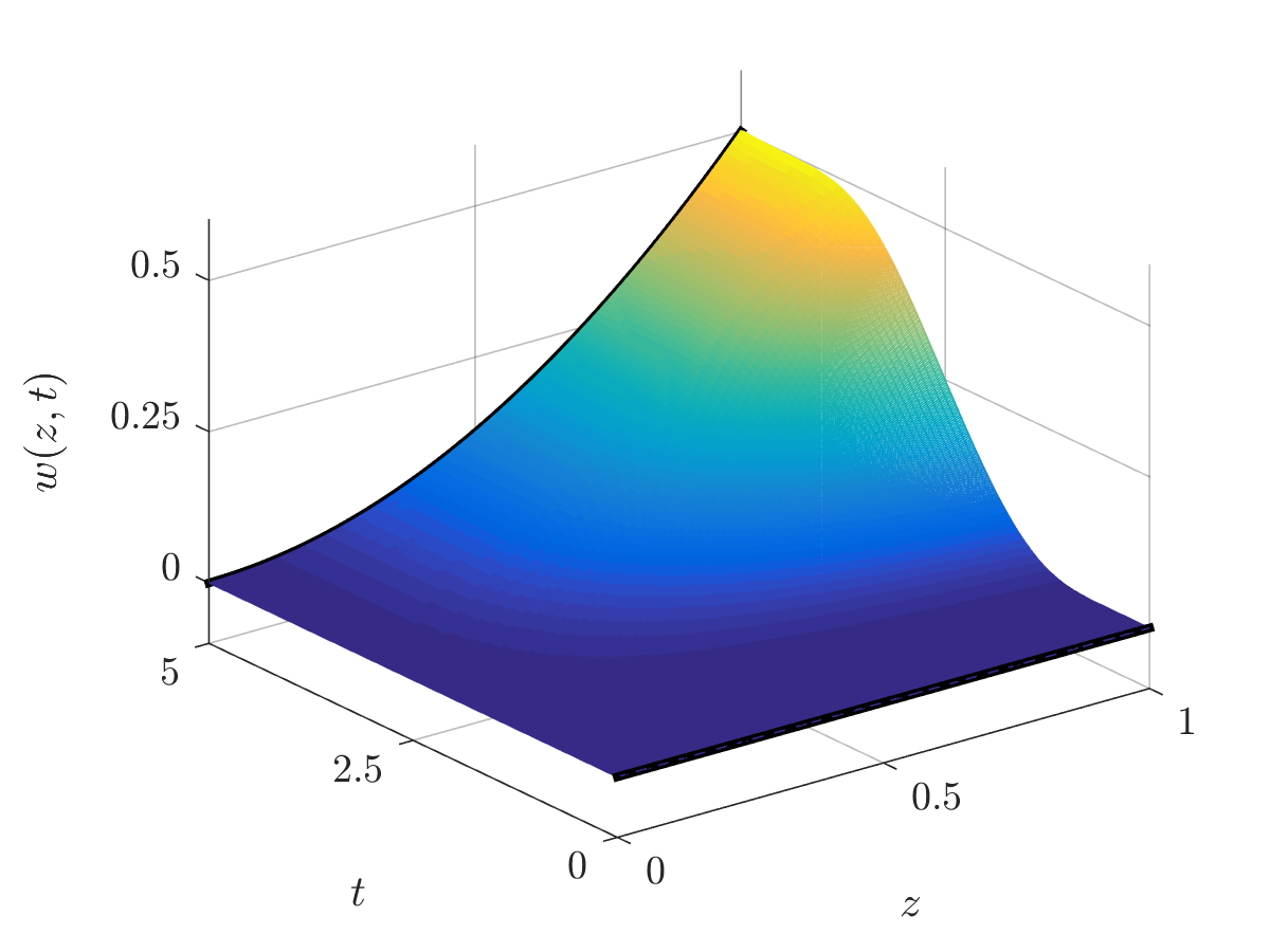
Figure 1: Deflection $w(z,t)$ of the beam

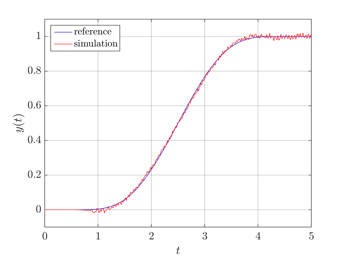
Figure 2: Bending moment $y(t)$ at the clamped boundary

Acknowledgements

This work has been supported by the Austrian Science Fund (FWF) under grant number P 29964-N32 and the Pro²Future competence center in the framework of the Austrian COMET-K1 programme under contract no. 854184.

References

- [1] M. Fliess, H. Mounier, P. Rouchon, and J. Rudolph, “Controllability and motion planning for linear delay systems with an application to a flexible rod,” in Proceedings 34th IEEE Conference on Decision and Control (CDC), 1995, pp. 2046–2051.
- [2] A. Lynch and J. Rudolph, “Flatness-based boundary control of a class of quasilinear parabolic distributed parameter systems,” International Journal of Control, vol. 75, no. 15, pp. 1219–1230, 2002.
- [3] J. Rudolph, Flatness Based Control of Distributed Parameter Systems. Aachen: Shaker Verlag, 2003.
- [4] T. Knüppel and F. Woittennek, “Control design for quasi-linear hyperbolic systems with an application to the heavy rope,” IEEE Transactions on Automatic Control, vol. 60, no. 1, pp. 5–18, 2015.
- [5] B. Laroche, P. Martin, and P. Rouchon, “Motion planning for the heat equation,” International Journal of Robust and Nonlinear Control, vol. 10, pp. 629–643, 2000.
- [6] M. Wagner, T. Meurer, and M. Zeitz, “K-summable power series as a design tool for feedforward control of diffusion-convection-reaction systems,” in Proceedings 6th IFAC Symposium on Nonlinear Control Systems (NOLCOS), 2004, pp. 147–152.
- [7] B. Laroche and P. Martin, “Motion planning for a 1-D diffusion equation using a Brunovsky-like decomposition,” in Proceedings 14th International Symposium on Mathematical Theory of Networks and Systems (MTNS), 2000.
- [8] P. Martin, R. Murray, and P. Rouchon, “Flat systems,” in Plenary Lectures and Mini-Courses, Proceedings 4th European Control Conference (ECC), G. Bastin and M. Gevers, Eds., 1997, pp. 211–264.
- [9] M. Fliess, H. Mounier, P. Rouchon, and J. Rudolph, “Systèmes linéaires sur les opérateurs de Mikusiński et commande d’une poutre flexible,” ESAIM: Proc., vol. 2, pp. 183–193, 1997.
- [10] J. Rudolph and F. Woittennek, “Motion planning for Euler-Bernoulli beams,” in Algebraic Methods in Flatness, Signal Processing and State Estimation, H. Sira-Ramirez and G. Silva-Navarro, Eds. Innovacion Editorial Lagares Mexico, 2003, ch. 8, pp. 131–148.
- [11] T. Meurer, J. Schröck, and A. Kugi, “Motion planning for a damped Euler-Bernoulli beam,” in Proceedings 49th IEEE Conference on Decision and Control (CDC), 2010, pp. 2566–2571.
- [12] W. Haas and J. Rudolph, “Steering the deflection of a piezoelectric bender,” in Proceedings 5th European Control Conference, 1999, pp. 3238–3243.
- [13] M. Wagner, T. Meurer, and A. Kugi, “Feedforward control design for the inviscid burger equation using formal power series and summation methods,” in Proceedings 17th IFAC World Congress, 2008, pp. 8743–8748.