Topological Susceptibility to High Temperatures via Reweighting

Abstract:

We measure the topological susceptibility of quenched QCD on the lattice at two high temperatures. For this, we define topology with the help of gradient flow and mitigate the statistical problem of topology at high temperatures using a reweighting technique. This allows us to enhance tunneling events between topological sectors and alleviate topological freezing. We quote continuum extrapolated results for the susceptibility at $2.5$ and $4.1~{}T_{\mathrm{c}}$ that agree well with the existing literature. We conclude that the method is feasible and can be extended to unquenched QCD with no conceptual problems.

1 Introduction

The axion [1, 2] is a hypothetical light scalar particle that could explain the origin of dark matter and solve the strong CP problem at the same time. It is introduced via the Peccei-Quinn mechanism [3, 4] that explains why the CP violating $\theta_{\mathrm{QCD}}$ term in the QCD Lagrangian is small. The corresponding particle on the other hand could be a candidate for dark matter in the Universe. In the last years, the high-energy physics community has put a lot of effort on the QCD axion, both in experiment and theory.

Given the interest on axions, theoretical predictions of its properties would be valuable. According to the Peccei-Quinn theory, dark-matter axion production is sensitive to the temperature dependence of the QCD topological susceptibility

$$\chi(T)=\int\mathrm{d}^{4}x\ \mathopen{}\mathclose{{}\left\langle q(x)q(0)}\right\rangle=\frac{1}{\beta V}\mathopen{}\mathclose{{}\left\langle Q^{2}}\right\rangle$$ (1)

up to temperatures of about $7~{}T_{\mathrm{c}}$ [5], where

$$q(x)=\frac{1}{64\pi^{2}}\epsilon_{\mu\nu\rho\sigma}F_{\mu\nu}^{a}(x)F_{\rho\sigma}^{a}(x)$$ (2)

is the topological charge density and $Q=\int\mathrm{d}^{4}x\ q(x)$ the topological charge.

At low temperatures, the value of the topological susceptibility is well established [6], while at high temperatures lattice calculations become very challenging. The main problem is that topologically non-trivial configurations, the so-called instantons, become very rare as the temperature increases. Therefore, sampling topological sectors with standard lattice techniques that rely on stochastic approaches fails at high temperatures. Another problem is topological freezing, which describes a deficiency of update algorithms that tend to get stuck in topological sectors.

There has been a lot of recent progress in studying topology at high temperatures [7, 8, 9, 10, 11, 12, 13]. One way [9, 13] to get to high temperatures is to start at a small temperature where instantons are not rare and differentially work up to high temperatures by studying fixed topological ensembles. As an alternative, we study topology directly at a given temperature by ameliorating the sampling problem using a reweighting approach. For simplicity, we constrained ourselves to the quenched approximation for developing this method, but we see no conceptual problems in applying the same technique to the unquenched case. Indeed, a very similar approach was recently applied to $N_{\mathrm{f}}=2+1$ QCD [14]. We first presented the method described here in Ref. [15], where the reader can find more details.

2 Reweighting Method

The difficulty that arises when measuring the topological susceptibility at high temperatures is twofold. On the one hand, the quantity is physically small, meaning that almost all configurations have trivial topology and a canonical sample has very little topological information. On the other hand, typical update algorithms tend to get stuck in topological sectors at fine lattices, preventing tunneling between topological sectors. The reweighting technique we developed has its roots in Refs. [16, 17, 18]. In the following, we summarize the basic ingredients of reweighting.

In the path-integral representation, the expectation value of an observable $O$ is given as

$$\mathopen{}\mathclose{{}\left\langle O}\right\rangle=\frac{\int\mathcal{D}U\mathrm{e}^{-S_{\mathrm{W}}[U]}O[U]}{\int\mathcal{D}U\mathrm{e}^{-S_{\mathrm{W}}[U]}},$$ (3)

where $S_{\mathrm{W}}$ is the standard Wilson action and $U$ denotes the gauge links. In lattice gauge theory, this quantity is approximated by generating lattice configurations distributed according to the probability distribution

$$\mathrm{d}P(U)=\frac{\mathrm{e}^{-S_{\mathrm{W}}[U]}\mathcal{D}U}{\int\mathcal{D}U\mathrm{e}^{-S_{\mathrm{W}}[U]}}.$$ (4)

In this way, Eq. (3) turns into

$$\mathopen{}\mathclose{{}\left\langle O}\right\rangle_{\mathrm{lat}}=\frac{1}{N}\sum_{i=1}^{N}O_{i},$$ (5)

where $i=1,\dots,N$ runs through the sample configurations.

The idea of reweighting is to rewrite Eq. (3) as

$$\mathopen{}\mathclose{{}\left\langle O}\right\rangle=\frac{\int\mathcal{D}U\mathrm{e}^{-S_{\mathrm{W}}[U]+W(\xi)}\mathrm{e}^{-W(\xi)}O[U]}{\int\mathcal{D}U\mathrm{e}^{-S_{\mathrm{W}}[U]+W(\xi)}\mathrm{e}^{-W(\xi)}}$$ (6)

and create a sample of configurations according to the now modified probability distribution

$$\mathrm{d}P_{\mathrm{rew}}(U)=\frac{\mathrm{e}^{-S_{\mathrm{W}}[U]+W(\xi)}\mathcal{D}U}{\int\mathcal{D}U\mathrm{e}^{-S_{\mathrm{W}}[U]+W(\xi)}}$$ (7)

that depends on the so-called reweighting function $W(\xi)$. In this way, we can artificially modify the weight of configurations with non-trivial topology. In order to compensate for this modified weight, we need to redefine the lattice expectation value as

$$\mathopen{}\mathclose{{}\left\langle O}\right\rangle=\frac{\sum_{i}^{N}O_{i}\mathrm{e}^{-W(\xi_{i})}}{\sum_{i}^{N}\mathrm{e}^{-W(\xi_{i})}}.$$ (8)

Note that Eqs. (3) and (8) form a mathematical identity if the algorithm tends to Eq. (7) and $N\to\infty$. The reweighting approach is therefore correct for any choice of the reweighting function. However, the particular choice is important to improve statistics in the case of topology at high temperatures as described in the next subsection. In the following, we use the HMC algorithm to update our configurations and implement the reweighting part in an additional Metropolis accept/reject step in terms of the change of $W$ after the standard Metropolis step in terms of the change of the Hamiltonian. For more details of the specific implementation we refer to Ref. [15].

2.1 Reweighting Variable

The key ingredient in the reweighting approach is the reweighting function $W(\xi)$ depending on the reweighting variable $\xi$. The idea is to enhance the number of topologically non-trivial configurations by giving them a larger weight, i.e., a large $W(\xi)$. Consequently, the reweighting variable $\xi$ needs be able to distinguish between different topological sectors. A natural choice would therefore be the topological charge

$$Q=\frac{1}{64\pi^{2}}\epsilon_{\mu\nu\rho\sigma}\sum_{x}\hat{F}^{a}_{\mu\nu}(x)\hat{F}^{a}_{\rho\sigma}(x),$$ (9)

where for the discretized field strength tensor we use an $\mathcal{O}\mathopen{}\mathclose{{}\left(a^{2}}\right)$ improved version. However, the topological charge is badly contaminated by UV fluctuations that add large contributions to the topological charge. In order to remove those, some amount of gradient flow [19, 20] is applied and we define the reweighting variable as

$$\xi=Q^{\prime}\equiv\mathopen{}\mathclose{{}\left|\frac{1}{64\pi^{2}}\epsilon_{\mu\nu\rho\sigma}\sum_{x}\mathopen{}\mathclose{{}\left(\hat{F}^{a}_{\mu\nu}(x)\hat{F}^{a}_{\rho\sigma}(x)}\right)_{t^{\prime}}}\right|,$$ (10)

where $t^{\prime}$ denotes a small amount of gradient flow. With small in this context we mean that UV fluctuations are removed, while dislocations, which are small concentrations of topological charge that are the intermediate steps between $Q=0$ and $Q=1$, are still present. Note that at high temperatures instantons are highly suppressed such that it is sufficient to only regard the $Q=1$ sector. Consequently, $Q^{\prime}$ distinguishes between $Q=0$ configurations, intermediate configurations with non-integer $Q$ (dislocations), and $Q=1$ configurations (instantons or calorons). Note that we here use the absolute value in the definition of $Q^{\prime}$ making use of the symmetry $Q\to-Q$.

2.2 Reweighting Function

In order to build the reweighting function, we perform a separate Markov chain where we change $W$ after each trajectory. A second, completely independent Markov chain is then used with $W$ fixed to extract physics information.

In this first, preparatory Markov chain, we first need to define the topological sectors that we want to include in the reweighting sample. As already discussed, at high temperatures it is adequate to only regard the $Q=1$ sector and we define the reweighting interval $\Omega_{\mathrm{rew}}=\mathopen{}\mathclose{{}\left\{Q^{\prime}\in\mathopen{}\mathclose{{}\left[0,1}\right]}\right\}$. The reweighting interval is further divided into $N_{\mathrm{int}}$ subintervals $0<Q^{\prime}_{1}<Q^{\prime}_{2}<\dots<Q^{\prime}_{\mathrm{int}}=1$ and $W$ is discretized on those points. Between the interval borders, $W$ is kept piecewise linear, starting with a constant function $W(Q^{\prime})\equiv 1$. We then perform the reweighted HMC updates described above. After each update, we assume that the current value of $Q^{\prime}$ is oversampled, because the algorithm managed to actually visit this $Q^{\prime}$. Consequently, it should become less probable to visit configurations with this $Q^{\prime}$ again and $W$ is lowered close to the $Q^{\prime}$ of the current configuration. A sketch of this procedure is shown in Fig. 1. For more details, we refer to Ref. [15].

In Fig. 2, the resulting reweighting function is shown for two different high temperatures above critical. Both functions show local minima close to $Q^{\prime}=0$ and $Q^{\prime}=1$ indicating the presence of topological sectors. In the intermediate $Q^{\prime}$ range, the $W$ function remains large so as to enhance tunneling events between sectors. Notice that $\exp\mathopen{}\mathclose{{}\left[-\mathopen{}\mathclose{{}\left(W(Q^{\prime}\simeq 1)-W(Q^{\prime}\simeq 0)}\right)}\right]$ provides an approximate estimate for the relative suppression of the $Q=1$ sector compared to the $Q=0$ sector and that this suppression is – as expected – much more severe for the higher temperature.

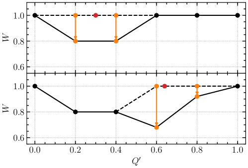
Figure 1: Sketch of how the reweighting function is built for $N_{\mathrm{int}}=5$. The red points indicate the measurement of $Q^{\prime}$ and the orange points the edges of the corresponding interval. The dashed line shows $W$ before the update, the solid line shows the updated $W$.

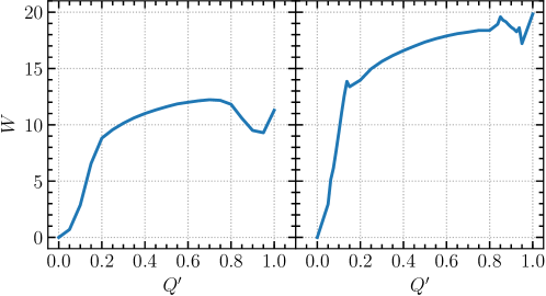
Figure 2: Left: $W(Q^{\prime})$ at $2.5~{}T_{\mathrm{c}}$. Right: $W(Q^{\prime})$ at $4.1~{}T_{\mathrm{c}}$.

3 Results and Conclusions

Ultimately we apply this strategy to SU(3) pure gauge theory at two high temperatures, namely $2.5$ and $4.1~{}T_{\mathrm{c}}$. We use lattices with three different lattice spacings using $N_{\tau}=6,8,10$ and aspect ratios of about $2.5$. For calculating the topological susceptibility via Eq. (1), we need to determine

$$\mathopen{}\mathclose{{}\left\langle Q^{2}}\right\rangle\equiv\frac{\sum_{i}\mathrm{e}^{-W\mathopen{}\mathclose{{}\left(Q^{\prime}_{i}}\right)}\uptheta\mathopen{}\mathclose{{}\left(Q_{i}^{2}(t)-Q_{\mathrm{thresh}}^{2}}\right)}{\sum_{i}\mathrm{e}^{-W\mathopen{}\mathclose{{}\left(Q^{\prime}_{i}}\right)}},$$ (11)

where $Q_{i}(t)$ is the topological charge after a large amount $t$ of gradient flow such that all UV fluctuations and dislocations are “flowed away”, and $Q_{\mathrm{thresh}}$ is a threshold to decide whether the configuration is an instanton or not. We then compare different flow depth and different thresholds.

Fig. 3 shows the continuum extrapolation at both temperatures for different choices of flow depth and $Q_{\mathrm{thresh}}$. We see that at coarse lattices the different topology definitions do not agree very well, while at finer lattices they do. Also in the continuum limit, the different choices give the same result. The continuum extrapolation is performed in the logarithm of the susceptibility because it is proportional to the exponential of the caloron action which has $\mathcal{O}\mathopen{}\mathclose{{}\left(a^{2}}\right)$ lattice corrections:

$$\chi\propto\exp\mathopen{}\mathclose{{}\left(-\mathopen{}\mathclose{{}\left[1-\mathcal{O}\mathopen{}\mathclose{{}\left(a^{2}T^{2}}\right)}\right]S}\right).$$ (12)

From this, a linear extrapolation in the logarithm of the susceptibility is well justified [21]. Our continuum extrapolated results are (using the $t=2.4a^{2}$ results with $Q_{\mathrm{thresh}}=0.7$)

$$\begin{split}\frac{\chi\mathopen{}\mathclose{{}\left(T=2.5~{}T_{\mathrm{c}}}\right)}{T_{\mathrm{c}}^{4}}&=2.22\times 10^{-4}\ \mathrm{e}^{\pm 0.18},\\ \frac{\chi\mathopen{}\mathclose{{}\left(T=4.1~{}T_{\mathrm{c}}}\right)}{T_{\mathrm{c}}^{4}}&=3.83\times 10^{-6}\ \mathrm{e}^{\pm 0.21}\end{split}$$ (13)

and agree well with the existing literature [8, 12].

In conclusion, we developed a reweighting approach to measure the topological susceptibility at high temperatures on the lattice. This method allows us to enhance tunneling between topological sectors where standard lattice techniques fail, and lets us measure the topological susceptibility directly also at high temperatures. We presented continuum extrapolated results for SU(3) pure Yang-Mills theory and see no conceptual problems for applying the same methods to QCD with fermions. Indeed, a similar technique was recently applied to $N_{\mathrm{f}}=2+1$ QCD [14].

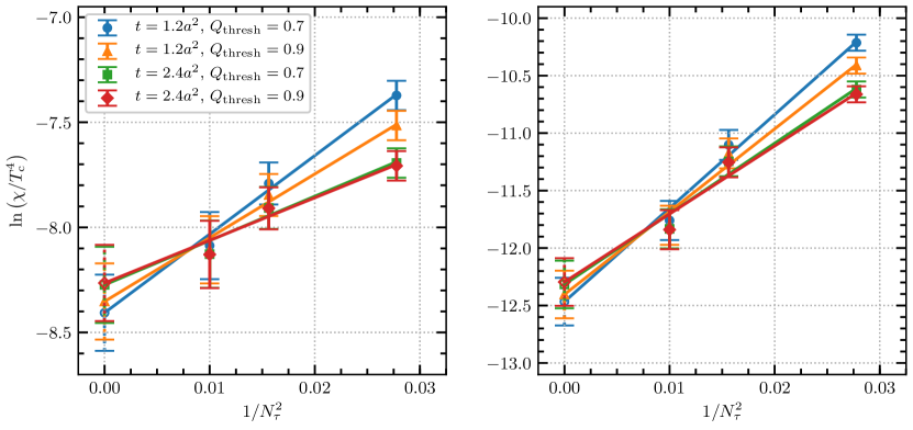
Figure 3: Left: linear continuum extrapolation in the logarithm of the susceptibility for two different flow depth $t$ and two different thresholds $Q_{\mathrm{thresh}}$ at $T=2.5~{}T_{\mathrm{c}}$. Right: the same at $T=4.1~{}T_{\mathrm{c}}$.

- [1] S. Weinberg, A New Light Boson?, Phys. Rev. Lett. 40 (1978) 223.
- [2] F. Wilczek, Problem of Strong p and t Invariance in the Presence of Instantons, Phys. Rev. Lett. 40 (1978) 279.
- [3] R. D. Peccei and H. R. Quinn, CP Conservation in the Presence of Instantons, Phys. Rev. Lett. 38 (1977) 1440.
- [4] R. D. Peccei and H. R. Quinn, Constraints Imposed by CP Conservation in the Presence of Instantons, Phys. Rev. D16 (1977) 1791.
- [5] G. D. Moore, Axion dark matter and the Lattice, EPJ Web Conf. 175 (2018) 01009.
- [6] G. Grilli di Cortona, E. Hardy, J. P. Vega and G. Villadoro, The QCD axion, precisely, JHEP 01 (2016) 034.
- [7] J. Frison, R. Kitano, H. Matsufuru, S. Mori and N. Yamada, Topological susceptibility at high temperature on the lattice, JHEP 09 (2016) 021.
- [8] E. Berkowitz, M. I. Buchoff and E. Rinaldi, Lattice QCD input for axion cosmology, Phys. Rev. D92 (2015) 034507.
- [9] Y. Taniguchi, K. Kanaya, H. Suzuki and T. Umeda, Topological susceptibility in finite temperature ( 2+1 )-flavor QCD using gradient flow, Phys. Rev. D95 (2017) 054502.
- [10] C. Bonati, M. D’Elia, M. Mariti, G. Martinelli, M. Mesiti, F. Negro et al., Axion phenomenology and -dependence from lattice QCD, JHEP 03 (2016) 155.
- [11] P. Petreczky, H.-P. Schadler and S. Sharma, The topological susceptibility in finite temperature QCD and axion cosmology, Phys. Lett. B762 (2016) 498.
- [12] S. Borsanyi, M. Dierigl, Z. Fodor, S. D. Katz, S. W. Mages, D. Nogradi et al., Axion cosmology, lattice QCD and the dilute instanton gas, Phys. Lett. B752 (2016) 175.
- [13] S. Borsanyi et al., Calculation of the axion mass based on high-temperature lattice quantum chromodynamics, Nature 539 (2016) 69.
- [14] C. Bonati, M. D’Elia, G. Martinelli, F. Negro, F. Sanfilippo and A. Todaro, Topology in full QCD at high temperature: a multicanonical approach, 1807.07954.
- [15] P. T. Jahn, G. D. Moore and D. Robaina, in pure-glue QCD through reweighting, Phys. Rev. D98 (2018) 054512.
- [16] B. A. Berg and T. Neuhaus, Multicanonical algorithms for first order phase transitions, Phys. Lett. B267 (1991) 249.
- [17] K. Kajantie, M. Laine, K. Rummukainen and M. E. Shaposhnikov, The Electroweak phase transition: A Nonperturbative analysis, Nucl. Phys. B466 (1996) 189.
- [18] F. Wang and D. P. Landau, Efficient, Multiple-Range Random Walk Algorithm to Calculate the Density of States, Phys. Rev. Lett. 86 (2001) 2050.
- [19] R. Narayanan and H. Neuberger, Infinite N phase transitions in continuum Wilson loop operators, JHEP 03 (2006) 064.
- [20] M. Lüscher, Trivializing maps, the Wilson flow and the HMC algorithm, Commun. Math. Phys. 293 (2010) 899.
- [21] P. T. Jahn, G. D. Moore and D. Robaina, Estimating Lattice Artifacts from Flowed SU(2) Calorons, 1805.11511.