On the 2D Dirac oscillator in the presence of vector and scalar potentials in the cosmic string spacetime in the context of spin and pseudospin symmetries

Abstract

The Dirac equation with both scalar and vector couplings describing the dynamics of a two-dimensional Dirac oscillator in the cosmic string spacetime is considered. We derive the Dirac-Pauli equation and solve it in the limit of the spin and the pseudo-spin symmetries. We analyze the presence of cylindrical symmetric scalar potentials which allows us to provide analytic solutions for the resultant field equation. By using an appropriate ansatz, we find that the radial equation is a biconfluent Heun-like differential equation. The solution of this equation provides us with more than one expression for the energy eigenvalues of the oscillator. We investigate these energies and find that there is a quantum condition between them. We study this condition in detail and find that it requires the fixation of one of the physical parameters involved in the problem. Expressions for the energy of the oscillator are obtained for some values of the quantum number $n$. Some particular cases which lead to known physical systems are also addressed.

1 Introduction

The study of the relativistic quantum dynamics of particles including electromagnetic interactions is an usual framework for studying properties of various physical systems. The mechanism used to describe these systems is a natural generalization of the coupling used in classical nonrelativistic quantum theory Book.2012.Itzykson . This coupling is implemented, for charged particles with charge $e$, through the so-called minimal coupling prescription, given in terms of the modification of the $4$-momentum operator, $p_{\mu}\rightarrow p_{\mu}-eA_{\mu}=\left(p_{0}-eA_{0},\mathbf{p}-e\mathbf{A}\right)$, where $A_{\mu}=\left(V(r),-\mathbf{A}\right)$ (with $\mathbf{A}$ being the vector potential and $V(r)$ being the scalar potential) represents the $4$-vector potential of the associated electromagnetic field. This transformation preserves the gauge invariance associated with the Maxwell’s equations. Another way to insert interaction in the dynamics of the particle is by including a scalar potential through a modification in the mass term as $M\rightarrow M+S(r)$. In this realization, the potential $S\left(r\right)$ is coupled like a scalar, different from the minimum prescription, where the potential is coupled as a time-like component of a 4-vector. Although there is some similarity between the scalar and vector couplings, they have different physical implications. Actually, the scalar coupling acts equally on particles and antiparticles. On the other hand, the vector coupling acts differently on particles and antiparticles. As a result, the energy of particle and antiparticle are not equals, so that bound states exist only for one of the two kinds of particles Book.2000.Greiner .

Interesting issues that should be investigated with the insertion of the couplings in the Dirac equation are the so-called the spin and the pseudo-spin symmetries PR.2005.414.165 . Basically, these symmetries occur when the couplings are composed by a vector $V(r)$ and a scalar $S(r)$ potential, under the assumption that $S(r)=V(r)$ ($S(r)=-V(r)$), which is the necessary condition for occurrence of exact spin (pseudo-spin) symmetry. The spin symmetry has been identified by studying heavy-light mesons PRL.2001.86.204 , single antinucleon spectra PRL.2003.91.262501 and dynamics of a light quark (antiquark) in the field of a heavy antiquark (quark) PR.2005.414.165 while that the pseudo-spin symmetry occurs in the motion of nucleons PR.1999.315.231 ; PR.2005.414.165 . In recent studies, both the spin and the pseudo-spin symmetries appear in several aspects concerning, for instance, the supersymmetry PLB.2011.699.309 ; JPA.2006.39.7737 , the Hartree-Fock theory PLB.2006.639.242 , the electrons in graphene PRA.2015.92.062137 and the interaction with a class of scalar and vector potentials AoP.2017.378.88 ; AoP.2016.364.99 ; EPJC.2015.75.321 ; AoP.2015.356.83 ; CTP.2015.64.637 ; JTAP.2015.9.15 ; IJMPA.2016.311650190 ; EPL.2007.77.20009 .

An important physical system that can be studied by including such terms of interactions in the Dirac equation is the Dirac oscillator JPA.1989.22.817 (for a detailed description of this model see Ref. Book.1998.Strange ). The Dirac oscillator is a kind of tensor coupling with a linear potential which in the nonrelativistic limit leads to the simple harmonic oscillator with a strong spin-orbit coupling. It was realized experimentally for the first time in 2013 by Franco-Villafañe et al. in PRL.2013.111.170405 . The Dirac oscillator is considered a natural model for studying properties of physical systems because it is exactly soluble. In the last years, several research have been developed in the context of this theoretical framework. For instance, it appears in the literature in the context of mathematical physics AoP.2014.351.13 ; JPA.2006.39.5125 ; EPL.2014.108.30003 ; PLA.2004.325.21 ; JPA.1997.30.2585 ; JPA.2005.38.1747 ; JPA.1991.24.667 ; PLB.2012.710.478 , nuclear physics PRC.2006.73.054309 ; PLA.2012.376.3475 ; PRC.2012.85.054617 ; AP.2005.320.71 , quantum optics JOB.2002.4.R1 ; OL.2010.35.1302 ; EPJB.2012.85.237 ; PRA.2007.76.041801 , supersymmetry JPA.1995.28.6447 ; JPA.2006.39.10909 ; CTP.2008.49.319 , theory of quantum deformations PLB.2014.731.327 ; PLB.2014.738.44 and noncommutativity PLA.2012.376.2467 ; IJTP.2013.52.441 ; IJTP.2012.51.2143 ; IJMPA.2011.26.4991 . Moreover, the Dirac oscillator embedded in a cosmic string background has inspired a great deal of research in last years EPJP.2018.133.409 ; EPJP.2012.127.82 ; GRG.2013.45.1847 ; PLA.2012.376.1269 ; PRA.2011.84.32109 ; AoP.2013.336.489 ; NPB.1989.328.140 ; PRL.1989.62.1071 ; PLA.2007.361.13 ; EPJC.2014.74.3187 .

In this work, we analyze in details the solutions of the Dirac equation with both scalar and vector interactions under the spin and the pseudo-spin symmetry limits in the cosmic string spacetime Book.2000.Vilenkin . Cosmic strings are topologically stable gravitational defects. According to the grand unified theories, these defects arise from a vacuum phase transition in the near universe. Recently, several studies have been developed in the theoretical context GRG.2018.50.125 ; PRD.2018.98.063519 ; IJMPA.2018.33.1850158 ; PRD.2017.96.024040 ; PRD.2018.97.085023 ; EPJC.2018.78.13 and also by evidence of cosmic strings PRL.2017.118.051301 ; PLB.2018.778.392 ; IJMPD.2018.27.1850094 ; MNRAS.2018.478.1132 . Cosmic strings are objects of studies of current interest because of the several important applications of topological features on physics systems in gravitation Book_Barriola_gravitation , condensed matter Book.2000.Vilenkin and cosmology Book_Shellard_1995 .

Our work is motivated by Ref. PRC.2002.65.054313 (see also Refs. PRC.1999.59.154 ; PRC.1998.58.R3065 ), where the spin and pseudospin symmetries in the relativistic mean field with a deformed potential are investigated. In this context, a relation between the deformed wave function and the spherical wave function was established at the spherical limit by using the transformation from the cylindrical coordinate into the polar coordinate. This relationship enables us to investigate the inclusion of cylindrical symmetrical potentials in the Dirac equation in other scenarios, such as the cosmic string. One advantage of using such symmetry limits in our work is that they allow us to decouple the first and second order differential equations for the spinor components (each obtained in the spin symmetry and pseudo-spin limits, respectively).

We organize the paper as follows: In Sec. 2, we derive the equation that governs the dynamics of a Dirac particle with the minimal, nonminimal and the scalar couplings in the cosmic string spacetime. In Sec. 3, we consider the Dirac equation written in terms of a set of coupled differential equations. We investigate the existence of particular solutions for the problem by assuming that the relativistic energy of the particle is its rest energy in both the spin and the pseudo-spin symmetries limits. In Sec. 4, we investigate the dynamics considering that the energy of the particle is different from its rest energy. To this end, we write down the Dirac equation in its quadratic form. We obtain the energies and the corresponded wave functions and discuss their physical validity. In Sec. 5, we address some particular solutions and compare them with previous results in the literature. Finally, the conclusions are presented in Sec. 6. Here, we use natural units such as $\hbar=c=1$.

2 The equation of motion

In this section, we derive the Dirac equation with scalar and vector couplings to study the motion of a Dirac oscillator in the cosmic string spacetime. We first define the spacetime background of an idealized cosmic string where the oscillator will move, followed by the most general interaction, which includes the potential of the Dirac oscillator. The interactions, however, are chosen in such a way that analytical solutions to the Dirac equation can be obtained.

The spacetime generated by a cosmic string is described by the following line element in cylindrical coordinates

$$ds^{2}=dt^{2}-dr^{2}-\alpha^{2}r^{2}d\varphi^{2}-dz^{2},$$ (1)

with $-\infty<(t,z)<\infty$, $r\geq 0$ and $0\leq\varphi\leq 2\pi$. The parameter $\alpha$ is related to the linear mass density $\tilde{m}$ of the string by $\alpha=1-4\tilde{m}$ and it runs in the interval $(0,1]$ and corresponds to a deficit angle $\gamma=2\pi(1-\alpha)$. Geometrically, the metric in Eq. (1) corresponds to a Minkowski spacetime with a conical singularity SPD.1977.22.312 .

One starts by considering the free Dirac equation, i.e., in the absence of interactions. The interaction will be included later. So, we have

$$\left(i\gamma^{\mu}\partial_{\mu}-M\right)\Psi=0,$$ (2)

where $\Psi$ is a four-component spinorial wave function. In order to work out in the curved spacetime, we must write the Dirac gamma matrices $\gamma^{\mu}$ in the Minkowskian spacetime (written in terms of local coordinates) in terms of global coordinates and subsequently include the spinor affine connection $\Gamma_{\mu}$. In other words, we must contract $\gamma^{\mu}$ with the inverse tetrad,

$$\gamma^{\mu}=e_{a}^{\mu}\gamma^{a},$$ (3)

satisfying the generalized Clifford algebra

$$\left\{\gamma^{\mu},\gamma^{\nu}\right\}=2g^{\mu\nu},$$ (4)

where $(\mu,\nu)=(0,1,2,3)$ are tensor indices and $(a,b)=(0,1,2,3)$ are tetrad indices. The matrices $\gamma^{a}=\left(\gamma^{0},\gamma^{i}\right)$ in Eq. (3) are the standard Dirac matrices in Minkowski spacetime, with

$$\gamma^{0}=\left(\begin{array}[]{rr}\mathbbm{1}&0\\ 0&\mathbb{-}\mathbbm{1}\end{array}\right),~{}~{}~{}\gamma^{i}=\left(\begin{array}[]{cc}0&\sigma^{i}\\ -\sigma^{i}&0\end{array}\right),\quad(i=1,2,3)$$ (5)

where $\sigma^{i}$ are the standard Pauli matrices and $\mathbbm{1}$ is the $2\times 2$ identity matrix. As we are interested on in a cosmic string, we need to write down the generalized Dirac equation in the curved spacetime background with a minimal coupling. Therefore, the relevant equation is

$$\left[i\gamma^{\mu}(\partial_{\mu}+\Gamma_{\mu})-e\gamma^{\mu}A_{\mu}-M\right]\Psi=0,$$ (6)

where $e$ is the electric charge and $A_{\mu}$ denotes the vector potential associated with the electromagnetic field. The spinor affine connection is often written as APPB.2010.41.1827

$$\Gamma_{\mu}=\frac{1}{8}\omega_{\mu ab}\left[\gamma^{a},\gamma^{b}\right],$$ (7)

where $\omega_{\mu ab}$ is the spin connection, given by

$$\omega_{\mu ab}=\eta_{ac}e_{\nu}^{c}e_{b}^{\tau}\Gamma_{\tau\mu}^{\nu}-\eta_{ac}e_{\nu}^{c}\partial_{\mu}e_{b}^{\nu}.$$ (8)

In (8), $\Gamma_{\tau\mu}^{\nu}$ are the Christoffel symbols and $\eta^{ab}$ is the metric tensor. By the means of the spin connection, we can construct a local frame using a basis tetrad which gives the spinors in the curved spacetime. Here, the basis tetrad $e_{a}^{\mu}$ is chosen to be PRD.2009.79.024008

$$e_{a}^{\mu}=\left(\begin{array}[]{cccc}1&0&0&0\\ 0&\cos\varphi&\sin\varphi&0\\ 0&-\sin\varphi/\alpha r&\cos\varphi/\alpha r&0\\ 0&0&0&1\end{array}\right),$$ (9)

satisfying the condition

$$e_{a}^{\mu}e_{b}^{\nu}\eta^{ab}=g^{\mu\nu}.$$ (10)

Using (9), the matrices $\gamma^{\mu}$ in Eq. (6) are written more explicitly as

$$\gamma^{0} = e_{0}^{t}\gamma^{0}\equiv\gamma^{t},$$ (11)

$$\gamma^{z} = e_{0}^{z}\gamma^{0}\equiv\gamma^{z},$$ (12)

$$\gamma^{1} = e_{a}^{1}\gamma^{a}\equiv\gamma^{r},$$ (13)

$$\gamma^{r} = e_{0}^{r}\gamma^{0}+e_{1}^{r}\gamma^{1}+e_{2}^{r}\gamma^{2},$$ (14)

$$= \gamma^{2}\cos\varphi+\gamma^{2}\sin\varphi,$$

$$\gamma^{2} = e_{a}^{2}\gamma^{a}\equiv\frac{\gamma^{\varphi}}{\alpha r},$$ (15)

$$\gamma^{\varphi} = e_{0}^{\varphi}\gamma^{0}+e_{1}^{\varphi}\gamma^{1}+e_{2}^{\varphi}\gamma^{2},$$ (16)

$$= -\gamma^{1}\sin\varphi+\gamma^{2}\cos\varphi.$$

Given the fact that the matrices in the curved space satisfy the condition $\nabla_{\mu}\gamma^{\mu}=0$, i.e., they are covariantly constant, for the specific basis tetrad (9), the affine spin connection is found to be

$$\boldsymbol{\Gamma}=\left(0,0,\Gamma_{\varphi},0\right),$$ (17)

with the non-vanishing element given by

$$\Gamma_{\varphi}=\frac{1}{2}\left(1-\alpha\right)\gamma_{1}\gamma_{2}.$$ (18)

We are interested on including potentials with cylindrical symmetry, in such a way the resulting system will have translational invariance along the $z$ direction. Then, we can discard the third direction and thus consider the Dirac oscillator in two spacial dimensions JPA.1989.22.817 (see also Ref. Book.1998.Strange ), assuming $p_{z}=0$ . This assumption allows us to reduce the four-component Dirac equation (6) to a two-component spinor equation. Moreover, according to the tetrad postulated APPB.2010.41.1827 , the $\gamma^{a}$ matrices could be any set of constant Dirac matrices. Thus, a convenient representation is the following PRD.1978.18.2932 ; NPB.1988.307.909 ; PRL.1989.62.1071

$$\gamma^{0}=\sigma^{z},\quad\beta\gamma^{1}=\sigma^{1},\quad\beta\gamma^{2}=s\sigma^{2},$$ (19)

where the parameter $s$, which is twice the spin value, can be introduced to characterize the two spin states, with $s=+1$ for spin “up” and $s=-1$ for spin “down”. In the representation (19), the matrices (11), (13) and (15) assume the following form:

$$\gamma^{0} = \beta=\sigma^{z},$$ (20)

$$\beta\gamma^{r} = \sigma^{r}=\left(\begin{array}[]{cc}0&e^{-is\varphi}\\ e^{is\varphi}&0\end{array}\right),$$ (23)

$$\beta\gamma^{\varphi} = s\sigma^{\varphi}=\frac{s}{\alpha r}\left(\begin{array}[]{cc}0&-ie^{-is\varphi}\\ ie^{is\varphi}&0\end{array}\right).$$ (26)

and Eq. (18) becomes

$$\Gamma_{\varphi}=-\frac{is}{2}\left(1-\alpha\right)\sigma^{z}.$$ (27)

Now, let us include the interactions into the Dirac equation (6). We consider the effective potential JPA.2007.40.6427 ; PRC.2012.86.052201

$$M\omega i\sigma^{z}\left(\beta\boldsymbol{\gamma}\cdot\mathbf{\hat{r}}\right)r+\frac{1}{2}\left(I+\sigma^{z}\right)\Sigma(r)+\frac{1}{2}\left(I-\sigma^{z}\right)\Delta(r),$$ (28)

with

$$\Delta(r) = V(r)-S(r),$$ (29)

$$\Sigma(r) = V(r)+S(r),$$ (30)

where

$$V(r) = V_{1}(r)+V_{2}(r)=\frac{\eta_{C_{1}}}{r}+\eta_{L_{1}}r,$$ (31)

$$S(r) = S_{1}(r)+S_{2}(r)=\frac{\eta_{C_{2}}}{r}+\eta_{L_{2}}r,$$ (32)

are cylindrically symmetric scalar and vector potentials. The first term in Eq. (28) represents the Dirac oscillator. In this manner, the time-independent Dirac equation (6) with energy $E$ can be written as

$$H_{D}\psi=E\psi,$$ (33)

where $\psi$ is a two-component spinor,

$$H_{D}= {}\beta\boldsymbol{\gamma}\cdot\left(\mathbf{p}_{\alpha}-i\boldsymbol{\Gamma}-iM\omega\beta\mathbf{r}\right)+\frac{1}{2}\left(I+\beta\right)\Sigma(r)$$

$$+\frac{1}{2}\left(I-\beta\right)\Delta(r)+\beta M,$$ (34)

is the Dirac Hamiltonian and

$$\mathbf{p}_{\alpha}=-i\mathbf{\nabla}_{\alpha}=-i\left(\frac{\partial}{\partial r}\mathbf{\hat{r}}+\frac{1}{\alpha r}\frac{\partial}{\partial\varphi}\mathbf{\hat{\varphi}}\right),$$ (35)

is the planar spatial part of the gradient operator in the metric (1).

We begin the study of the particle motion by looking for first order solutions of the Eq. (33). For this purpose, we write the Eq. (33) as follows,

$$ie^{-is\varphi}\left[-\frac{\partial}{\partial r}+M\omega r+\frac{is}{\alpha r}\frac{\partial}{\partial\varphi}-\frac{\left(1-\alpha\right)}{2\alpha r}\right]\psi_{2}=\\ \left[E-M-\Sigma(r)\right]\psi_{1},$$ (36a)

and

$$ie^{+is\varphi}\left[-\frac{\partial}{\partial r}-M\omega r-\frac{is}{\alpha r}\frac{\partial}{\partial\varphi}-\frac{\left(1-\alpha\right)}{2\alpha r}\right]\psi_{1}=\\ \left[E+M-\Delta(r)\right]\psi_{2},$$ (36b)

and we consider the solutions as

$$\psi=\begin{pmatrix}\psi_{1}\\ \psi_{2}\end{pmatrix}=\begin{pmatrix}\sum\limits_{m}f(r)\,e^{im\varphi}\\ \sum\limits_{m}ig(r)\,e^{i\left(m+s\right)\varphi}\end{pmatrix},$$ (37)

with $m=0,\pm 1,\pm 2,\pm 3,\ldots$ being the quantum angular momentum number. The substitution of (37) into (36a) and (36b) gives the following set of coupled differential equations:

$$\left(\frac{d}{dr}+s\frac{J_{\alpha}^{-}}{r}-M\omega r\right)g_{m}={} \left[E-M-\Sigma(r)\right]f_{m},$$ (38)

$$\left(-\frac{d}{dr}+s\frac{J_{\alpha}^{+}}{r}-M\omega r\right)f_{m}={} \left[E+M-\Delta(r)\right]g_{m}.$$ (39)

where

$$J_{\alpha}^{\pm}={} \frac{1}{\alpha}\left[m+s\Theta^{\pm}+\frac{s}{2}(1-\alpha)\right],$$ (40)

where $\Theta^{+}=0$ and $\Theta^{-}=1$. The reason why we are using superscripts ($\pm$) in Eq. (40) will be clarified in the next section. If we consider that $\Delta\left(r\right)=0$ and $E=-M$ or $\Sigma\left(r\right)=0$ and $E=+M$, the solutions of Eqs. (38) and (39) represent a particular solution for the problem, which is excluded from the Sturm-Liouville problem. In other words, such solutions would not be part of those obtained by solving the second-order differential equation obtained from Eq. (33). The procedure of imposing that either $\Delta\left(r\right)=0$ or $\Sigma\left(r\right)=0$ in Eqs. (38) and (39), respectively, is known in the literature as the exact limits of spin and pseudo-spin symmetries PR.2005.414.165 . These conditions are taken into account in the next section.

3 Particular solutions and the analysis of the spin and the pseudo-spin symmetries

In this section, we solve the system of first-order radial differential equations obtained in the previous section by imposing either the exact limits of spin and pseudo-spin symmetries. Once we find the solutions, we must verify that they are physically acceptable solutions. As mentioned above, the exact limit of the spin symmetry occurs when $\Delta\left(r\right)=0$ ($V(r)=S(r)$ in Eq. (29)), while that the exact limit of the pseudospin symmetry is achieved by setting $\Sigma(r)=0$ ($V(r)=-S(r)$ in Eq. (30)). In what follows, the superscript ($+$) holds for the spin symmetry and ($-$) holds for the pseudo-spin symmetry. In these limits, the solutions are related to the up and down components of the spinor in Eq. (37), respectively.

In order to obtain the particular solutions, let us look for the bound state solutions which obey the following normalization condition,

$$\int_{0}^{\infty}\left(|f_{m}(r)|^{2}+|g_{m}(r)|^{2}\right)rdr=1\;.$$ (41)

We assume $E=\pm M$, as it was mentioned above.

3.1 The exact spin symmetry

Here, the particular solutions for the bound states are obtained by considering $\Delta(r)=0$ along with the assumption $E=-M$ in both Eqs. (38) and (39). Therefore, we have

$$\left(\frac{d}{dr}+s\frac{J_{\alpha}^{-}}{r}-M\omega r\right)g_{m}(r)={} -2\left[M+S(r)\right]f_{m}\left(r\right),$$ (42)

$$\left(-\frac{d}{dr}+s\frac{J_{\alpha}^{+}}{r}-M\omega r\right)f_{m}(r)={} 0.$$ (43)

Their solutions are written as

$$f_{m}(r)={} a_{1}r^{sJ_{\alpha}^{+}}e^{-\frac{1}{2}M\omega r^{2}},$$ (44)

$$g_{m}(r)={} r^{-sJ_{\alpha}^{-}}e^{\frac{1}{2}M\omega r^{2}}$$

$$\times\left[a_{1}\left(M\omega\right)^{-\frac{1}{2}s\left(J_{\alpha}^{+}+J_{\alpha}^{-}\right)-\frac{3}{2}}\Gamma_{(a,b,c)}+a_{2}\right],$$ (45)

with

$$\Gamma_{(a,b,c)}=\eta_{C}\left(M\omega\right)^{\frac{3}{2}}\Gamma_{\left(a\right)}+\eta_{L}\left(M\omega\right)^{\frac{1}{2}}\Gamma_{\left(b\right)}+M^{2}\omega\Gamma_{\left(c\right)},$$ (46)

where

$$\Gamma_{\left(a\right)} = \Gamma\left[\frac{1}{2}s\left(J_{\alpha}^{+}+J_{\alpha}^{-}\right),\,M\omega r^{2}\right],$$ (47)

$$\Gamma_{\left(b\right)} = \Gamma\left[\frac{1}{2}s\left(J_{\alpha}^{+}+J_{\alpha}^{-}\right)+1,\,M\omega r^{2}\right],$$ (48)

$$\Gamma_{\left(c\right)} = \Gamma\left[\frac{1}{2}s\left(J_{\alpha}^{+}+J_{\alpha}^{-}\right)+\frac{1}{2},\,M\omega r^{2}\right],$$ (49)

are upper incomplete Gamma functions Book.1972.Abramowitz , $a_{1}$ and $a_{2}$ are constants. Let us discuss the solutions (44) and (45). Since $e^{-\frac{1}{2}M\omega r^{2}}$ dominates over $r^{sJ_{\alpha}^{+}}$ for any value of $sJ_{\alpha}^{+}$, the solution $f_{m}(r)$ in Eq. (44) converges as $r\rightarrow 0$ and $r\rightarrow\infty$. On the other hand, as the incomplete Gamma functions $\Gamma_{(a,b,c)}$ always diverge, so $g_{m}(r)$ in (45) will only converge as $r\rightarrow 0$ if $a_{1}=0$, yielding $f_{m}(r)=0$. The resulting solution are

$$\left[\begin{array}[]{c}f_{m}(r)\\ g_{m}(r)\end{array}\right]=a_{2}\left(\begin{array}[]{c}0\\ 1\end{array}\right)r^{-sJ_{\alpha}^{-}}e^{\frac{1}{2}M\omega r^{2}},\quad\begin{cases}s=\pm 1,\\ a_{1}=0.\end{cases}$$ (50)

As $M\omega>0$ in (50), there are no values of $sJ_{\alpha}^{-}$ for which the functions are square-integrable. In this case, we can therefore conclude right away that for $E=-M$ and exact spin symmetry there is no bound state solution.

3.2 Exact pseudo-spin symmetry

In this case, we impose $\Sigma(r)=0$ and $E=M$ in both Eqs. (38) and (39). Thus, we obtain

$$\left(\frac{d}{dr}+s\frac{J_{\alpha}^{-}}{r}-M\omega r\right)g_{m}\left(r\right)={} 0,$$ (51)

$$\left(-\frac{d}{dr}+s\frac{J_{\alpha}^{+}}{r}-M\omega r\right)f_{m}\left(r\right)={} 2\left[M+S(r)\right]g_{m}(r).$$ (52)

Their solutions are given by

$$f_{m}(r)={} b_{1}r^{sJ_{\alpha}^{+}}e^{-\frac{1}{2}M\omega r^{2}}$$

$$\times\left[b_{1}-b_{2}(-M\omega)^{\frac{1}{2}s\left(J_{\alpha}^{-}+J_{\alpha}^{+}\right)-\frac{3}{2}}\Gamma\left(d,e,f\right)\right],$$ (53)

$$g_{m}(r)={} b_{2}r^{-sJ_{\alpha}^{-}}e^{\frac{1}{2}M\omega r^{2}},$$ (54)

where $b_{1}$ and $b_{2}$ are constants, and

$$\Gamma_{(d,e,f)}=M^{2}\omega\Gamma_{\left(d\right)}-\text{$\eta_{C}$}\left(-M\omega\right)^{\frac{3}{2}}\Gamma_{\left(e\right)}-\text{$\eta_{L}$}\left(-M\omega\right)^{\frac{1}{2}}\Gamma_{\left(f\right)},$$ (55)

with

$$\Gamma_{\left(d\right)}={} \Gamma\left[\frac{1}{2}-\frac{1}{2}s\left(J_{\alpha}^{-}+J_{\alpha}^{+}\right),-M\omega r^{2}\right],$$ (56)

$$\Gamma_{\left(e\right)}={} \Gamma\left[-\frac{1}{2}s\left(J_{\alpha}^{-}+J_{\alpha}^{+}\right),-M\omega r^{2}\right],$$ (57)

$$\Gamma_{\left(f\right)}= \Gamma\left[1-\frac{1}{2}s\left(J_{\alpha}^{-}+J_{\alpha}^{+}\right),-M\omega r^{2}\right].$$ (58)

Again, the incomplete Gamma functions $\Gamma_{(d,e,f)}$ in Eq. (53) always diverge, so that a normalized solution requires that $b_{2}=0$. In such a case, the function $f_{m}(r)$ is square-integrable only for $sJ_{\alpha}^{+}\geq 0$. The physically acceptable solution is

$$\left[\begin{array}[]{c}f_{m}(r)\\ g_{m}(r)\end{array}\right]=b_{1}r^{sJ_{\alpha}^{+}}e^{-\frac{1}{2}M\omega r^{2}}\left(\begin{array}[]{c}0\\ 1\end{array}\right),\quad\begin{cases}sJ_{\alpha}^{+}\geq 0,\\ a_{1}=0.\end{cases}$$ (59)

Therefore, we can conclude that for the case $E=M$ along with the exact pseudo-spin symmetry there is a bound state solution. Here, the existence of a particular bound state solution is guaranteed only for $M\omega>0$. However, there are other models in the literature where this quantity can assume any value, so that bound states solutions are allowed for both the spin and pseudospin symmetry limits AoP.362.196.2015 .

4 The Dirac-Pauli equation and the analysis of both the spin and the pseudo-spin symmetries

In this section, we study the dynamics for the case $E\neq\pm M$. For this purpose, it is more convenient to work with the Eq. (33) in its quadratic form. In our analysis, we shall see that because of the shape of the potential (28), the solutions for the radial equation are given in terms of biconfluent Heun functions and the energy levels of the oscillator will be determined only after imposing some quantum conditions.

To obtain the quadratic form of the Dirac equation (33), we multiply it by the matrix operator

$$\beta\boldsymbol{\gamma}\cdot\left(\mathbf{p}_{\alpha}-i\boldsymbol{\Gamma}-iM\omega\beta\mathbf{r}\right)+\beta M+E+\frac{1}{2}\left(\beta-\mathbbm{1}\right)\Sigma(r)\\ -\frac{1}{2}\left(\mathbbm{1}+\beta\right)\Delta(r),$$ (60)

leading to

$$-\nabla_{\alpha}^{2}\psi-\frac{(1-\alpha)s\sigma^{z}}{i\alpha^{2}r^{2}}\frac{\partial}{\partial\varphi}+\frac{(1-\alpha)^{2}}{4\alpha^{2}r^{2}}+M^{2}\omega^{2}r^{2}\psi\\ -2M\omega\left\{\sigma^{z}+\frac{s}{\alpha}\left[\frac{1}{i}\frac{\partial}{\partial\varphi}-\frac{s}{2}\left(1-\alpha\right)\sigma^{z}\right]\right\}\psi\\ -\Sigma(r)\Delta(r)\psi+\left(E+M\right)\Sigma(r)\psi+\left(E-M\right)\Delta(r)\psi\\ +\left(M^{2}-E^{2}\right)\psi-\frac{1}{2}i\sigma^{r}\left\{\frac{d}{dr}\left[\Sigma(r)+\Delta(r)\right]\right\}\psi\\ -\frac{1}{2}\sigma^{\varphi}\left\{\frac{d}{dr}\left[\Sigma\left(r\right)-\Delta(r)\right]\right\}\psi=0,$$ (61)

where $\nabla_{\alpha}^{2}=\partial_{r}^{2}+(1/r)\partial_{r}+(1/\alpha^{2}r^{2})\partial_{\varphi}^{2}$ is the planar spatial part of the Laplace-Beltrami operator in the metric (1). By inserting the solutions (37) into Eq. (61), we obtain the following set of two coupled radial differential equations of second-order:

$$-\frac{d^{2}f(r)}{dr^{2}}-\frac{1}{r}\frac{df(r)}{dr}+\frac{\left(J_{\alpha}^{+}\right)^{2}}{r^{2}}f(r)+M^{2}\omega^{2}r^{2}f(r)\\ -2M\omega\left(sJ_{\alpha}^{+}+1\right)f(r)-\Sigma(r)\Delta(r)f(r)\\ +\left(E+M\right)\Sigma(r)f(r)+\left(E-M\right)\Delta(r)f(r)+\left(M^{2}-E^{2}\right)f(r)\\ +\left[\frac{d\Delta\left(r\right)}{dr}\right]g(r)=0,$$ (62)

and

$$-\frac{d^{2}g(r)}{dr^{2}}-\frac{1}{r}\frac{dg(r)}{dr}+\frac{\left(J_{\alpha}^{-}\right)^{2}}{r^{2}}g(r)+M^{2}\omega^{2}r^{2}g(r)\\ -2M\omega\left(sJ_{\alpha}^{-}-1\right)g(r)-\Sigma(r)\Delta(r)g(r)\\ +\left(E+M\right)\Sigma(r)g(r)+\left(E-M\right)\Delta(r)g(r)+\left(M^{2}-E^{2}\right)g(r)\\ -\left[\frac{d\Sigma(r)}{dr}\right]f(r)\,=0.$$ (63)

Notice that these two equations are coupled via the last terms and the spin and pseudospin symmetry limits uncouple them. So, here and henceforth we employ the following approach. For the spin symmetry limit, we solve the problem by considering the upper component of the spinor and denotes it by $f^{+}$ (i.e., $+$ labels the spin symmetry solution) and for the pseudospin symmetry limit, we consider the lower component and denotes it by $g^{-}$ (i.e., $-$ labels the pseudospin symmetry solution).

4.1 The analysis of both the spin and the pseudo-spin symmetries

When we take into account the exact limits of spin and symmetries in Eqs. (62) and (63), each component of the spinor satisfies

$$-\frac{d^{2}f^{+}(r)}{dr^{2}}-\frac{1}{r}\frac{df^{+}\left(r\right)}{dr}+\frac{\left(J_{\alpha}^{+}\right)^{2}}{r^{2}}f^{+}\left(r\right)+\varpi^{2}r^{2}f^{+}(r)\\ +\frac{{a}^{+}}{r}f^{+}(r)+b^{+}rf^{+}(r)-\left(k^{+}\right)^{2}f^{+}(r)=0,$$ (64)

and

$$-\frac{d^{2}g^{-}(r)}{dr^{2}}-\frac{1}{r}\frac{dg^{-}\left(r\right)}{dr}+\frac{\left(J_{\alpha}^{-}\right)^{2}}{r^{2}}g^{-}\left(r\right)+\varpi^{2}r^{2}g^{-}(r)\\ +\frac{a^{-}}{r}g^{-}(r)+b^{-}rg^{-}(r)-\left(k^{-}\right)^{2}g^{-}(r)=0,$$ (65)

where

$$\left(k^{\pm}\right)^{2}=E^{2}-M^{2}+2M\omega\left(sJ_{\alpha}^{\pm}\pm 1\right),$$ (66)

$\varpi=M\omega$, $a^{\pm}=2(E\pm M)\eta_{C}$ and $b^{\pm}=2(E\pm M)\eta_{L}$. The differential equations (64) and (65) can be placed in an convenient mode using, respectively, the following solutions:

$$f^{+}(x)={} {x}^{\left|J_{\alpha}^{+}\right|}e{{}^{-\frac{1}{2}({x}^{2}+\xi_{L}^{+}x)}}y^{+}(x),$$ (67)

$$g^{-}(x)={} {x}^{\left|J_{\alpha}^{-}\right|}e{{}^{-\frac{1}{2}({x}^{2}+\xi_{L}^{-}x)}}y^{-}(x),$$ (68)

where $x=\sqrt{\varpi}r$ and ${y}^{\pm}(x)$ satisfies

$$x\left[{y}^{\pm}(x)\right]^{\prime\prime}+\left[\mathbb{J}^{\pm}-2{x}^{2}-\xi_{L}^{\pm}x\right]\left[{y}^{\pm}(x)\right]^{\prime}\\ +\left[\left(\Delta^{\pm}-\mathbb{J}^{\pm}-1\right)x-\frac{1}{2}\left(\mathbb{J}^{\pm}\xi_{L}^{\pm}+2\xi_{C}^{\pm}\right)\right]{y}^{\pm}\left(x\right)=0,$$ (69)

where

$$\Delta^{\pm}= {}\frac{\left(\xi_{L}^{\pm}\right)^{2}}{4}+\frac{\left(k^{\pm}\right)^{2}}{\varpi},$$ (70)

$$\mathbb{J}^{\pm}= {}2\left|J_{\alpha}^{\pm}\right|+1,$$ (71)

$\xi_{C}^{\pm}={a}^{\pm}/\sqrt{\varpi}$ and $\xi_{L}^{\pm}=b^{\pm}/\sqrt{\varpi^{3}}$. Equation (69) is a homogeneous, linear, second-order, differential equations defined in the complex plane. The solutions of these equations are given in terms of the biconfluent Heun functions by Book.2010.NIST ; Book.Ronveaux1995

$$f^{+}(x)={} e{{}^{-\frac{1}{2}({x}^{2}+\xi_{L}^{+}x)}}\Big{[}c_{1}{x}^{\left|J_{\alpha}^{+}\right|}\mathit{N}^{+}\left(2\,{\left|J_{\alpha}^{+}\right|},\xi_{L}^{+},\Delta^{+},2\xi_{C}^{+},x\right)$$

$$+c_{2}{x}^{-\left|J_{\alpha}^{+}\right|}\mathit{N}^{+}\left(-2{\left|J_{\alpha}^{+}\right|},\xi_{L}^{+},\Delta^{+},2\xi_{C}^{+},\,x\right)\Big{]},$$ (72)

$$g^{-}(x)={} e{{}^{-\frac{1}{2}({x}^{2}+\xi_{L}^{-}x)}}\Big{[}c_{1}{x}^{\left|J_{\alpha}^{-}\right|}\mathit{N}^{-}\left(2\,{\left|J_{\alpha}^{-}\right|},\xi_{L}^{-},\,\Delta^{-},2\xi_{C}^{-},x\right)$$

$$+c_{2}{x}^{-\left|J_{\alpha}^{-}\right|}\mathit{N}^{-}\left(-2{\left|J_{\alpha}^{-}\right|},\xi_{L}^{-},\Delta^{-},2\xi_{C}^{-},x\right)\Big{]},$$ (73)

where

$$\mathit{N}^{\pm}\left(2\,{\left|J_{\alpha}^{\pm}\right|},\,\xi_{L}^{\pm},\,\Delta^{\pm},2\,\xi_{C}^{\pm},\,x\right)\\ =\sum\limits_{q=0}^{\infty}\frac{\mathcal{A}_{q}^{\pm}\left(2\,{\left|J_{\alpha}^{\pm}\right|},\,\xi_{L}^{\pm},\,\Delta^{\pm},\,2\,\xi_{C}^{\pm}\right)}{\left(1+2\,{\left|J_{\alpha}^{\pm}\right|}\right)_{q}}\frac{x^{q}}{q!}.$$ (74)

The coefficients of the series are given by

$$\mathcal{A}_{0}^{\pm}={} 1,$$ (75)

$$\mathcal{A}_{1}^{\pm}={} \frac{1}{2}\left[2\,\xi_{C}^{\pm}+\xi_{L}^{\pm}\left(1+2\,{\left|J_{\alpha}^{\pm}\right|}\right)\right],$$ (76)

$$\mathcal{A}_{q+2}^{\pm}= \left\{\left(q+1\right)\xi_{L}^{\pm}+\frac{1}{2}\left[2\xi_{C}^{\pm}+\xi_{L}^{\pm}\left(1+2{\left|J_{\alpha}^{\pm}\right|}\right)\right]\right\}\mathcal{A}_{q+1}^{\pm}$$

$$-\left(q+1\right)\left(q+1+2\,{\left|J_{\alpha}^{\pm}\right|}\right)$$

$$\times\left[\Delta^{\pm}-2(\,{\left|J_{\alpha}^{\pm}\right|}-1-q)\right]\mathcal{A}_{q}^{\pm},$$ (77)

and

$$\left(1+2\,{\left|J_{\alpha}^{\pm}\right|}\right)_{q}=\frac{\Gamma\left(q+2\,{\left|J_{\alpha}^{\pm}\right|}+1\right)}{\Gamma\left(2\,{\left|J_{\alpha}^{\pm}\right|}+1\right)}.$$ (78)

From the recursion relation (77), the function

$$\mathit{N}^{\pm}(2\,{\left|J_{\alpha}^{\pm}\right|},\,\xi_{L}^{\pm},\,\Delta^{\pm},2\,\xi_{C}^{\pm},\,x)$$

becomes a polynomial of degree $n$, if and only if, the two following conditions are imposed Book.Ronveaux1995 ; JCAM.1991.37.161 :

$$\Delta^{\pm}-2\left(1+\,{\left|J_{\alpha}^{\pm}\right|}\right)=2n,\;\;n=0,1,2,\ldots,$$ (79)

$$\mathcal{A}_{n+1}^{\pm}=0.$$ (80)

In this case, the $\left(n+1\right)$th coefficient in the series expansion is a polynomial of degree $n$ in $2\,\xi_{C}^{\pm}$. When $2\,\xi_{C}^{\pm}$ is a root of this polynomial, the $\left(n+1\right)$th and subsequent coefficients cancel and the series truncates, resulting in a polynomial form of degree $n$ for the solution $\mathit{N}^{\pm}\left(2\,{|J_{\alpha}^{\pm}|},\,\xi_{L}^{\pm},\,\Delta^{\pm},\,2\,\xi_{C}^{\pm},\,x\right)$. From the condition (79), we extract the following expressions involving the energy $E_{nm}^{\pm}$:

$$\left(E_{nm}^{\pm}\right)^{2}-M^{2}={} 2M\omega\left[n+\left|J_{\alpha}^{\pm}\right|-sJ_{\alpha}^{\pm}+2\Theta^{\pm}\right]$$

$$-\frac{\eta_{L}^{2}}{M^{2}\omega^{2}}\left(E_{nm}^{\pm}\pm M\right)^{2},$$ (81)

We notice in Eq. (81) the absence of the parameter $\eta_{C}$. This steams from the fact that these expressions do not represent the energies of the system in its present form. Actually, the condition (80) allows us to establish a quantum condition that links the energy and others physical quantities, including $\eta_{C}$ PRC.2012.86.052201 ; AoP.2014.347.130 ; JMP.2015.56.092501 . As a result, it is possible to express the energy in terms of all the physical parameters involved in the problem, namely, $\eta_{C}$, $\eta_{L}$, $M$, and $\omega$. We emphasize that that, a priori, we are free to choose which parameter we want to fix. Here, such a quantum condition is established through the frequency $\omega$ of the system. Therefore, we now label $\omega$ as $\omega_{nm}$. Before performing the procedure, let us consider the solution (74) up to second-order in $x$ of the expansion, namely,

$$\mathit{N}^{\pm}\left(2\,{|J_{\alpha}^{\pm}|},\,\xi_{L}^{\pm},\,\Delta^{\pm},\,2\,\xi_{C}^{\pm},\,x\right)=\frac{\mathcal{A}_{0}^{\pm}}{\left(1+2\,{|J_{\alpha}^{\pm}|}\right)_{0}}\\ +\frac{\mathcal{A}_{1}^{\pm}}{\left(1+2\,{|J_{\alpha}^{\pm}|}\right)_{1}}x+\frac{\mathcal{A}_{2}^{\pm}}{\left(1+2\,{|J_{\alpha}^{\pm}|}\right)_{2}}\frac{x^{2}}{2!}+\ldots$$ (82)

with

$$\mathcal{A}_{0}^{\pm}={} 1,$$ (83)

$$\mathcal{A}_{1}^{\pm}={} \,\frac{1}{2}\left[2\,\xi_{C}^{\pm}+\xi_{L}^{\pm}\mathbb{J}^{\pm}\right],$$ (84)

$$\mathcal{A}_{2}^{\pm}={} \xi_{L}^{\pm}\left[\xi_{C}^{\pm}+\frac{1}{2}\xi_{L}^{\pm}\mathbb{J}^{\pm}\right]+\left[\,\xi_{C}^{\pm}+\frac{1}{2}\xi_{L}^{\pm}\mathbb{J}^{\pm}\right]^{2},$$ (85)

Thus, Eq. (82) reads

$$\mathit{N}^{\pm}\left(2\,{|J_{\alpha}^{\pm}|},\,\xi_{L}^{\pm},\,\Delta^{\pm},\,2\,\xi_{C}^{\pm},\,x\right)=1+\left[\frac{\xi_{L}^{\pm}\mathbb{J}^{\pm}+2\,\xi_{C}^{\pm}}{2\left(2\,{\left|J_{\alpha}^{\pm}\right|}+1\right)}\right]x\\ +\left[\frac{\xi_{L}^{\pm}\left(\xi_{C}^{\pm}+\frac{1}{2}\xi_{L}^{\pm}\mathbb{J}^{\pm}\right)+\,\left(\xi_{C}^{\pm}+\frac{1}{2}\xi_{L}^{\pm}\mathbb{J}^{\pm}\right)^{2}-2n\mathbb{J}^{\pm}}{\left(2\,{\left|J_{\alpha}^{+}\right|}+1\right)\left(2\,{\left|J_{\alpha}^{+}\right|}+2\right)}\right]x^{2}\\ +\ldots.$$ (86)

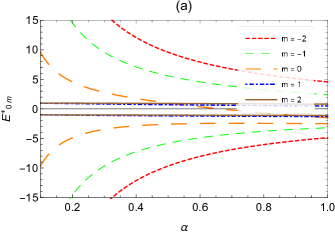
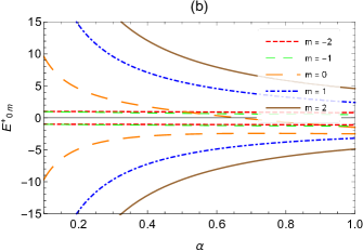
Figure 1: (Color online) Illustration of the energy eigenvalues in the spin symmetry limit, $E^{+}_{0m}$, as a function of the parameter $\alpha$. (a) $s=1$ and (b) $s=-1$. We use $M=1$, $\eta_{C}=1$ and $\eta_{L}=1$. In (a) the energies of the states with $m<1$ become larger for $\alpha\to 0$ whereas for $\alpha=1$ the differences between the energy levels decrease as well as the energy values. For the states with $m\geqslant 1$ (dot-dashed blue and solid brown lines), the energies change very slowly and are non-degenerate. In (b) the opposite of (a) occurs: the states with $m\geqslant 0$ are more energetic for $\alpha\to 0$ and less energetic for $\alpha=1$.

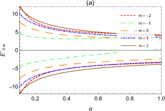
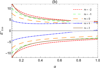
Figure 2: (Color online) Illustration of the energy eigenvalues in the pseudospin symmetry limit, $E^{-}_{0m}$, as a function of the parameter $\alpha$. In (a) the plot for $s=1$ and (b) for $s=-1$. We use $M=1$, $\eta_{C}=1$ and $\eta_{L}=1$. The energies of the states corresponding to a given value of $m$ near $\alpha=0$ in (a) and (b) are more energetic while near $\alpha=1$ the differences between the energy levels decrease as well as their respective values.

Now let us determine the quantum condition mentioned above. For the condition (80), we must investigate $\mathcal{A}_{n+1}^{\pm}=0$. For simplicity, we consider only the case $n=0$, which requires that $\mathcal{A}_{1}^{\pm}=0$ in Eq. (84). This requires us to solve the equation

$$2\,\frac{{a}^{\pm}}{\sqrt{\varpi}}+\frac{b^{\pm}}{\sqrt{\varpi^{3}}}\mathbb{J}^{\pm}=0,$$ (87)

which provides the following frequencies related to the ground state of the system:

$$\omega_{0m}^{\pm}=-\frac{\eta_{L}}{2M\,\eta_{C}}\,\mathbb{J}^{\pm}.$$ (88)

However, Eq. (88) will only be an acceptable quantum condition if $\eta_{L}/\eta_{C}<0$ to ensure that the frequencies $\omega_{0m}^{\pm}$ are positive. Thus, respective energies corresponding to the ground state are

$$E_{0m}^{\pm}={} \frac{4M\,\eta_{C}^{2}}{1+\left(\mathbb{J}^{\pm}\right)^{2}}\left[\mp 1(\pm)\sqrt{1+\frac{\left(\mathbb{J}^{\pm}\right)^{2}}{4M^{2}\eta_{C}^{2}}Q_{0m}^{\pm}}\right],$$ (89)

where

$$Q_{0m}^{\pm}={} \left[\frac{\eta_{L}}{\,\eta_{C}}\left({\left|J_{\alpha}^{\pm}\right|}-sJ_{\alpha}^{\pm}+2\Theta^{\pm}\right)\mathbb{J}^{\pm}-\frac{4M^{2}\,\eta_{C}^{2}}{\left(\mathbb{J}^{\pm}\right)^{2}}+M^{2}\right]$$

$$\times\left[1+\frac{\left(\mathbb{J}^{\pm}\right)^{2}}{4\,\eta_{C}^{2}}\right].$$ (90)

In (89), the notation $(\pm)$ refers to the particle and antiparticle energies. The energies in Eq. (89) now depend on all the physical parameters involved in the problem. In Figs. 1 and 2, we plot the profile of these energies as a function of the parameter $\alpha$. In both plots we clearly see that the energy levels of the particle and antiparticle belong to the same spectrum and, moreover, there is no channel that allows the spontaneous creation of particles because none of the lines of the spectrum cross each other.

5 Particular cases

In this section, we study particular solutions of problem solved in the previous section. Namely, we will investigate three cases. For the first two, the solutions of the resulting equations are given in terms of biconfluent Heun functions whereas the third, which will not involve scalar and vectorial interactions, will be given in terms of the confluent hypergeometric function.

Let us then return to Eq. (69) and solve it for the particular case $\eta_{L}=0$. The resulting equation governs the dynamics of a two-dimensional Dirac oscillator interacting with the potential $\eta_{C}/r$. In this case, the solutions are given by

$$\tilde{f}^{+}(x)={} \mathit{\tilde{c}}_{1}{x}^{\left|J_{\alpha}^{+}\right|}e{{}^{-\frac{1}{2}{x}^{2}}}\mathit{\tilde{N}}^{+}\left(2{\left|J_{\alpha}^{+}\right|},0,\Delta^{+},2\xi_{C}^{+},x\right)$$

$$+\mathit{\tilde{c}}_{2}\,{x}^{-\left|J_{\alpha}^{+}\right|}e{{}^{-\frac{1}{2}{x}^{2}}}\mathit{\tilde{N}}^{+}\left(-2\,{\left|J_{\alpha}^{+}\right|},0,\Delta^{+},2\xi_{C}^{+},x\right),$$ (91)

$$\tilde{g}^{-}(x)={} \mathit{\tilde{c}}_{1}{x}^{\left|J_{\alpha}^{-}\right|}e{{}^{-\frac{1}{2}{x}^{2}}}\mathit{\tilde{N}}^{-}\left(2{\left|J_{\alpha}^{-}\right|},0,\Delta^{-},2\xi_{C}^{-},x\right)$$

$$+\mathit{\tilde{c}}_{2}\,{x}^{-\left|J_{\alpha}^{-}\right|}e{{}^{-\frac{1}{2}{x}^{2}}}\mathit{\tilde{N}}^{-}\left(-2{\left|J_{\alpha}^{-}\right|},0,\Delta^{-},2\xi_{C}^{-},x\right).$$ (92)

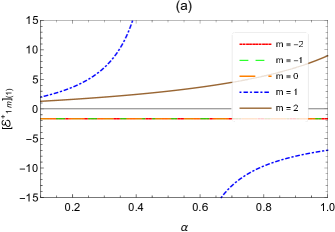
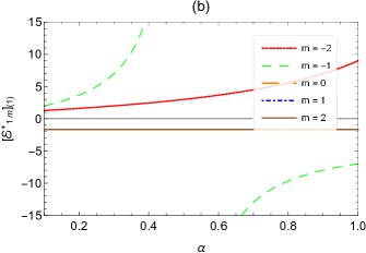
Figure 3: (Color online) Illustration of the energy levels in the spin symmetry limit, $\left[\mathcal{E}_{1m}^{+}\right]_{p}$, as a function of the parameter $\alpha$ for the particular case when $\eta_{L}=0$. In (a) the plot for $s=1$ and (b) for $s=-1$. We use $M=1$ and $\eta_{C}=1$. In (a) the energies are degenerate for $m=-2,-1,0$. Energy is not defined in $\alpha=0.5$ when $m=1$ (dashed green line). The energy value for $m=2$ (solid brown line) and $\alpha\to 0$ increases while near $\alpha=1$ it decreases. The characteristics present in (b) are equivalent to (a) by changing $m$ by $-m$.

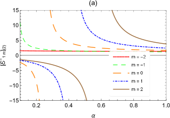
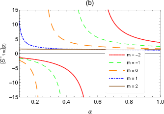
Figure 4: (Color online) Illustration of the energy levels in the pseudo-spin symmetry limit, $\left[\mathcal{E}_{1m}^{-}\right]_{p}$, as a function of the parameter $\alpha$ for the particular case when $\eta_{L}=0$. In (a) the plot for $s=1$ and (b) for $s=-1$. We use $M=1$ and $\eta_{C}=1$. In (a) the energy of the states are not defined when the parameter $\alpha$ is $0.25$ (dashed-long orange line), 0.42 (dashed-dot blue line) and 0.59 (solid brown line). The energy of the state with $m=-2$ (dot red line) changes very slowly and it shows no degeneracy. The spectrum is more energetic near the points of singularity and less energetic near $\alpha=0.1$ and $\alpha=1$, respectively, except the $m=-1$ curve (dashed green line), which is more energetic only near $\alpha=0.1$. The characteristics manifested in (b) are equivalent to (a) by changing $m$ by $-m$.

Then, using the condition (79), we find the energies

$$\left(\mathcal{E}_{nm}^{\pm}\right)^{2}-M^{2}={} 2M\left(n+{\left|J_{\alpha}^{\pm}\right|}-sJ_{\alpha}^{\pm}+2\Theta^{\pm}\right)\tilde{\omega}_{nm}^{\pm},$$ (93)

Moreover, from condition (80), we consider again $\mathcal{A}_{n+1}^{\pm}=0$ for $n=0$, and solve it for $\tilde{\varpi}_{0m}^{\pm}$. One can thus verify that it is not possible to extract a physically acceptable expression for $\tilde{\varpi}_{0m}^{\pm}$. Consequently, $n=0$ is not an allowed value for the quantum number and we need to solve $\mathcal{A}_{n+1}^{\pm}=0$ for $n=1$. Thus, we have

$$\tilde{\varpi}_{1m}^{\pm}={} \frac{2\eta_{C}^{2}}{M}\frac{\left(\mathcal{E}_{1m}^{\pm}+M\right)^{2}}{\mathbb{J}^{\pm}},$$ (94)

Substituting (94) into (93) and solving these equations for $\mathcal{E}_{1m}^{\pm}$, we find

$$\left[\mathcal{E}_{1m}^{+}\right]_{p}={} \left(\frac{1+\frac{2\eta_{C}^{2}}{\mathbb{J}_{+}}\left(1+\mathbb{J}_{+}-2sJ_{\alpha}^{+}\right)}{1-\frac{2\eta_{C}^{2}}{\mathbb{J}_{+}}\left(1+\mathbb{J}_{+}-2sJ_{\alpha}^{+}\right)}\right)M,$$ (95a)

$$\left[\mathcal{E}_{1m}^{+}\right]_{ap}={} -M,$$ (95b)

and

$$\left[\mathcal{E}_{1m}^{-}\right]_{p} =M,$$ (96a)

$$\left[\mathcal{E}_{1m}^{-}\right]_{ap} =-\left(\frac{1+\frac{2\eta_{C}^{2}}{\mathbb{J}^{-}}\left(\mathbb{J}^{-}-2sJ_{\alpha}^{-}+5\right)}{1-\frac{2\eta_{C}^{2}}{\mathbb{J}^{-}}\left(\mathbb{J}^{-}-2sJ_{\alpha}^{-}+5\right)}\right)M,$$ (96b)

where the subscripts $$p ap \mathcal{E}_{0m}^{\pm}\neq\pm M \left[\mathcal{E}_{1m}^{+}\right]_{ap} \left[\mathcal{E}_{1m}^{-}\right]_{p} \alpha s=+1 m=-2,-1,0 s=-1 m=0,1,2 m=-2 s=+1 m=2 s=-1$$ and refer to the energies of the particle and antiparticle, respectively. As we are studying the dynamics for which , the energies and are not allowed energies for the particle. The profiles of the energies (95a) and (96b) as a function of the parameter are shown in Figs. 3 and 4, respectively. We can observe in Fig. 3(a) () the presence of degeneracy for , while in Fig. 3(b) (), the degeneracy occurs for . In Fig. 4, the spectrum of the states with (Fig. 4(a) for ) and with (Fig. 4(b) for ) change very slowly and are non-degenerate.

The second particular case is when $\eta_{C}=0$. In this case, the system consists of a Dirac oscillator interacting with a linear potential, $\eta_{L}r$. Thus, the solutions of Eq. (69) is again given in terms of the Heun functions,

$$\bar{f}^{+}(x)={} e{{}^{-\frac{1}{2}({x}^{2}+\xi_{L}^{+})}}\Big{[}\mathit{\bar{c}}_{1}\,{x}^{\left|J_{\alpha}^{+}\right|}\mathit{\bar{N}}^{+}\left(2\,{\left|J_{\alpha}^{+}\right|},\xi_{L}^{+},\,\Delta^{+},0,x\right)$$

$$+\mathit{\bar{c}}_{2}\,{x}^{-\left|J_{\alpha}^{+}\right|}\mathit{\bar{N}}^{+}\left(-2\,{\left|J_{\alpha}^{+}\right|},\xi_{L}^{+},\Delta^{+},0,x\right)\Big{]},$$ (97)

$$\bar{g}^{-}(x)={} e{{}^{-\frac{1}{2}({x}^{2}+\xi_{L}^{-})}}\Big{[}\mathit{\bar{c}}_{1}\,{x}^{\left|J_{\alpha}^{-}\right|}\mathit{\bar{N}}^{-}\left(2\,{\left|J_{\alpha}^{-}\right|},\xi_{L}^{-},\,\Delta_{-},0,x\right)$$

$$+\mathit{\bar{c}}_{2}\,{x}^{-\left|J_{\alpha}^{-}\right|}\mathit{\bar{N}}^{-}\left(-2\,{\left|J_{\alpha}^{-}\right|},\xi_{L}^{-},\Delta_{-},0,x\right)\Big{]},$$ (98)

and the energies are given by

$$\left(\bar{E}_{nm}^{\pm}\right)^{2}-M^{2}={} 2M\bar{\omega}\left(n+\left|J_{\alpha}^{\pm}\right|-sJ_{\alpha}^{\pm}+1+\Theta^{\pm}\right)$$

$$-\frac{\eta_{L}^{2}}{M^{2}\bar{\omega}^{2}}\left(\bar{E}_{nm}^{\pm}\pm M\right)^{2},$$ (99)

Note that energies (99) are identical to those given in Eq. (81). However, the frequency $\bar{\omega}$ is not the same. The difference between them is just the imposition established by the condition (80). For $n=0$, we obtain the frequencies

$$\bar{\omega}_{0m}^{\pm}={} 0,$$ (100)

By substituting (100) into the respective energies (99), we find

$$\bar{E}_{0m}^{\pm} =\mp M(\pm)M.$$ (101)

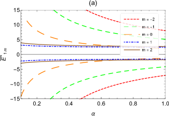
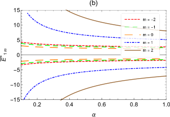
Figure 5: (Color online) The energy $\bar{E}_{1m}^{+}$ as a function of the parameter $\alpha$. (a) $s=1$, (b) $s=-1$. We use $M=1$ and $\eta_{L}=1$. In (a) the plot for $s=1$ and (b) for $s=-1$. We see clearly that the spectrum of the states are more energetic near $\alpha=0.1$ and less energetic near $\alpha=1$.

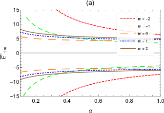
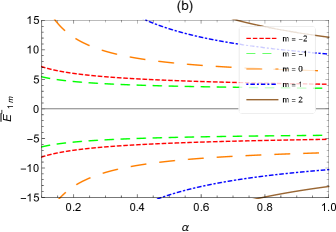
Figure 6: (Color online) The energy $\bar{E}_{1m}^{-}$ as a function of the parameter $\alpha$. We use $M=1$ and $\eta_{L}=1$. In (a) the plot for $s=1$ and (b) for $s=-1$. The states are more energetic near $\alpha=0.1$ and less energetic near $\alpha=1$.

For $n=1$, we have

$$\bar{\omega}_{1m}^{\pm}={} \frac{1}{M}\left[\eta_{L}^{2}\left(1+\,\frac{\mathbb{J}^{\pm}}{2}\right)\left(\bar{E}_{1m}^{\pm}\pm M\right)^{2}\right]^{\frac{1}{3}},$$ (102)

and the energies are given by

$$\left(\bar{E}_{1m}^{\pm}\right)^{2}-M^{2}={} 2M\bar{\omega}_{1m}^{\pm}\left(n+\left|J_{\alpha}^{\pm}\right|-sJ_{\alpha}^{\pm}+2\Theta^{\pm}\right)$$

$$-\frac{\eta_{L}^{2}}{M^{2}\left(\bar{\omega}_{1m}^{\pm}\right)^{2}}\left(\bar{E}_{1m}^{\pm}+M\right)^{2},$$ (103)

with $\bar{\omega}_{1m}^{\pm}$ given in Eq. (102). For this particular case, it is verified that Eq. (103) presents four energy eigenvalues being two for each type of symmetry limit considered. However, only two of them are physically acceptable. The profiles of the energies $\bar{E}_{1m}^{+}$ and $\bar{E}_{1m}^{-}$ are plotted as a function of the parameter $\alpha$ for $s=1$ and $s=-1$ in Figs. 5 and 6, respectively. We can see that both particle and antiparticle belong to the same spectrum and contains no degeneracy. In Fig. 5(a), we clearly observe that the states with $m>0$ are more affected by the curvature while in Fig. 5(b) this occurs for the states with $m>0$. These same characteristics are also present in Fig. 6, the only difference is that the spacing between each level as well as their respective energy values are larger when compared with the spectra of the Fig. 5.

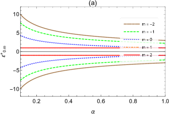
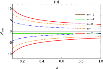
Figure 7: (Color online) The energy $\epsilon_{0m}^{+}$ as a function of the parameter $\alpha$. In (a) the plot for $s=1$ and (b) for $s=-1$. We use $M=1$. In (a), the states with $m\leqslant 0$ are more affected by curvature while the states with $m\geqslant 1$ are degenerate and are not affected by curvature. In (b), we have the situation opposite to (a): the states with $m\geqslant 0$ are most affected by curvature and states with $m\leqslant-1$ are degenerate and are not affected by curvature.

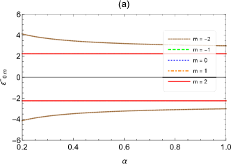
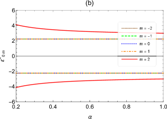
Figure 8: (Color online) The energy $\epsilon_{0m}^{-}$ as a function of the parameter $\alpha$. In (a) the plot for $s=1$ and (b) for $s=-1$. We use $M=1$. The only non-degenerate states affected by curvature are those with $m\leqslant-2$ in (a) and $m\geqslant 2$ in (b). All states with $m<2$ are not affected by curvature.

Finally, the last case we want to discuss in that in which $\eta_{L}=\eta_{C}=0$ in Eq. (69). In this case, the solutions (72) and (73) take the form

$$f^{+}(x)={} {x}^{\left|J_{\alpha}^{+}\right|}e{{}^{-\frac{1}{2}{x}^{2}}}F^{+}(x),$$ (104)

$$g^{-}(x)={} {x}^{\left|J_{\alpha}^{-}\right|}e{{}^{-\frac{1}{2}{x}^{2}}}F^{-}(x),$$ (105)

where $x=\sqrt{\varpi}r$ and $F^{\pm}(x)$ satisfies the Kummer differential equation Book.1972.Abramowitz ; Book.2010.NIST

$$\left({F}^{\pm}\right)^{\prime\prime}(x)+\left(\frac{2\left|J_{\alpha}^{+}\right|+1}{x}-2{x}\right)\left({F}^{\pm}\right)^{\prime}(x)\\ +\left[\breve{\Delta}^{\pm}-\left(2\left|J_{\alpha}^{+}\right|+2\right)\right]\left({F}^{\pm}\right)(x)=0,$$ (106)

whose general solution is known to be

$$F^{\pm}(x)={} a_{n}{\mathrm{M}\left(\frac{1}{2}+\frac{\left|J_{\alpha}^{\pm}\right|}{2}-\frac{\breve{\Delta}^{\pm}}{4},1+\left|J_{\alpha}^{\pm}\right|,{x}^{2}\right)}$$

$$+b_{n}x^{-2\left|J_{\alpha}^{\pm}\right|}\mathrm{M}\left(\frac{1}{2}-\frac{\left|J_{\alpha}^{\pm}\right|}{2}-\frac{\breve{\Delta}^{\pm}}{4},1-\left|J_{\alpha}^{\pm}\right|,{x}^{2}\right),$$ (107)

In the above equations, $\mathrm{M}$ is the Kummer function Book.1972.Abramowitz ; Book.2010.NIST . For this particular case, if we write the condition (79) in the form

$$\frac{1}{2}+\frac{\left|J_{\alpha}^{\pm}\right|}{2}-\frac{\breve{\Delta}^{\pm}}{4}=-n^{\prime},$$ (108)

with $n^{\prime}=0,1,2,3,...$, where $\breve{\Delta}^{\pm}=\left(\breve{k}^{\pm}\right)^{2}/M\omega$ and $\left(\breve{k}^{\pm}\right)^{2}=\left(\epsilon_{nm}^{\pm}\right)^{2}-M^{2}+2M\omega\left(sJ_{\alpha}^{\pm}\pm 1\right)$, the energies of the oscillator are obtained. Since $V(r)=S(r)=0$, spin and pseudo-spin symmetries are now absent, and signals ($\pm$) in Eq. (108) are only used to represent the function $f^{+}(x)$, $g^{-}(x)$ (components of $\psi$ of Eq. (61) with positive and negative energy, respectively) of the particle. In this way, the eigenvalues of Eq. (106) are given by

$$\left(\epsilon_{nm}^{\pm}\right)^{2}-M^{2} =M\omega\left[2n+\mathbb{J}^{\pm}+1\right]-2M\omega\left(sJ_{\alpha}^{\pm}\pm 1\right),$$ (109)

and the unnormalized bound state wave functions are

$$f^{+}(x)={} {x}^{\left|J_{\alpha}^{+}\right|}e{{}^{-\frac{1}{2}{x}^{2}}\mathrm{M}\left(-n,1+\left|J_{\alpha}^{+}\right|,\,{x}^{2}\right)},$$ (110)

$$g^{-}(x)={} {x}^{\left|J_{\alpha}^{-}\right|}e{{}^{-\frac{1}{2}{x}^{2}}\mathrm{M}\left(-n,1+\left|J_{\alpha}^{-}\right|,\,{x}^{2}\right)}.$$ (111)

The energies in Eq. (109) (for $n=0$ and $s=\pm 1$) are plotted as a function of the parameter $\alpha$ in Figs. 7 e 8, respectively. For a particle with $s=1$ (Fig. 7(a)), all states with $m>0$ are degenerate and are not affected by curvature while with $s=-1$ (Fig. 7(b)), this characteristic occurs for the states with $m<0$. On the other hand, for an antiparticle with $s=1$ (Fig. 8(a)), only the state with $m=-2$ is non-degenerate while with $s=-1$ (Fig. 8(b)), only the state with $m=2$ is non-degenerate. In Ref. EPJC.74.3187.2014 , the Dirac 2D oscillator interacting with the Aharonov-Bohm potential in the time space of the cosmic string was studied in the context of self-adjoint extensions. In the absence of the Aharonov-Bohm field, the resulting equation corresponding to the regular solution (Eq. 46) of Ref. EPJC.74.3187.2014 reproduces the Eq. (109).

6 Conclusion

In this paper, we have studied the dynamics of a 2D Dirac oscillator interacting with cylindrically symmetric scalar and vector potentials in the space-time of the cosmic string. The problem was solved taking into account the spin and pseudospin symmetry exact limits through two stages. First we have solved the Dirac equation by looking for first order solutions. We used an appropriate ansatz for the Dirac equation and obtained a system of coupled first order differential equations. We investigated this system and verified that it admits physically acceptable particular solutions, i.e., bound states solutions, only for the pseudo-spin symmetry exact limit, $\Sigma=0$ and $E=M$. In the second moment, we have constructed and solved the Dirac equation in its quadratic form, which excludes the $E\neq\pm M$ cases from its solutions. For this case, we shown that the resulting radial differential equation is the biconfluent Heun equation. We studied the series solution of this equation as well as its asymptotic behavior at infinity and at the origin and found two conditions (Eqs. (79) and (80)) to make the series a polynomial. The use of these two conditions allowed us to obtain expressions for the energies corresponding to fixed values of $n$. In particular, we obtained the expression corresponding to the state with $n=0$, which is given by Eq. (89). We investigate how the curvature affects the energies. For this intent, we have plotted it as a function of the parameter $\alpha$ for each of the limits of symmetries and spin element projection considered. In the case of the energy obtained for the spin symmetry limit (Eq. (89) with superscript $+$), we have shown that for $s=1$ the states with $m<1$ become more energetic when $\alpha\to 0$ while for $\alpha=1$ the differences between the energy levels as well as the respective energy values decrease. For the states with $m\geqslant 1$, the energies change very slowly and are non-degenerate. When the spin element is $s=-1$, we have verified that the effects are opposite to those for $s=1$, namely, the states with $m\geqslant 0$ are more energetic for $\alpha\to 0$ and less energetic for $\alpha=1$. These characteristics were also observed in the graph of the energies obtained in the pseud-spin symmetry limit (Eq. (89) with superscript $-$). For both $s=\pm 1$, the energies of the states corresponding to a given value of $m$ when $\alpha\to 0$ are more energetic while for $\alpha=1$ the differences between the energy levels decrease as well as their respective energy values.

We also investigated some special cases for the solution of the Eq. (61). In the first case, we have assumed the vanishing of the linear potential by imposing $\eta_{L}=0$. We obtained the energies (Eqs. (95a)-(95b) and (96a)-(96b)) and plot them as a function of the parameter $\alpha$ for both $s=\pm 1$. However, we have shown that the energies (95b) and (96a) are not allowed. In the energy profile (95a) for $s=1$, the energies of states with $m\leqslant 0$ are degenerate. In particular, when $\alpha=0.5$, the state energy with $m=1$ is not defined. We also have observed that the energy values of the state with $m=2$ when $\alpha\to 0.$ increases while for $\alpha=1$ it decreases. It also was verified that these same characteristics are present in the graphic for $s=-1$. In the plot of the energy given by Eq. (95b) for $s=\pm 1$, other important characteristics were manifested, and these are absent in the plot of Eq. (95a). For $s=1$, the energy of the states are not defined for $\alpha$ equal to $0.25$, $0.42$ and $0.59$. The spectrum is more energetic for $\alpha\to 0$ and $\alpha=1$, except the $m=-1$ curve, in which is more energetic only for $\alpha\to 0$. We have found that energy of the state with $m=-2$ changes very slowly and are non-degenerate. We have also found that these characteristics are present in the graphic for $s=-1$.

In the second particular case investigated, we have assumed $\eta_{C}=0$ and, as for the first case, four energy eigenvalues were found, but only two of them are physically acceptable because of the requirement that $E\neq\pm M$. For this case, we have not found energies with a given values of $m$ and $\alpha$ that are not allowed. The graphs of the energies (for $s=\pm 1$) as a function of the $\alpha$ for both spin and pseudo-spin symmetry limits revealed that they are more energetic for $\alpha\to 0$ and less energetic for $\alpha=1.0$. The only difference is that the spacing between the energies of the states for a fixed $m$ in the spin symmetry limit are greater than those in the spin symmetry limit.

In the last particular case studied, we have assumed $\eta_{L}=\eta_{C}=0$. For this system, the resulting radial equation was a equation Kummer differential equation type. We obtained the energy spectrum ($\epsilon_{nm}^{\pm}$ in Eq. (109)) and we plotted it as a function of the $\alpha$ for both $s=\pm 1$. In the graph of the energy $\epsilon_{0m}^{+}$ for $s=1$, we have verified that the states with $m>0$ are degenerate while for $s=-1$ this occurs for states with $m<0$. In the graph of the energy $\epsilon_{0m}^{-}$, we have found that only the states with $m=-2$ (for $s=1$) and with $m=2$ (for $s=-1$) are non-degenerate. A feature present in all energy profiles, including the general case, is the absence of channel that allows creation of particles, and also no crossings of lines, which guarantees that particle and antiparticle belong to the same spectrum.

As a final remark, we would like to mention that the model addressed here can be applied to other systems, especially those in condensed matter physics. This is due to the fact that linear defects in condensed matter, such as disclinations and dislocations in solids, can be studied through the same approach used to treat a cosmic string Book.2000.Vilenkin . A possible application would be an adaptation of the model used to investigate how the quantum dots and antidots, with the pseudoharmonic interaction and under the influence of external magnetic and Aharonov-Bohm potential are influenced by the presence of a screw dislocation as that studied in Ref. PLA.2016.380.3847 in the context of spin and pseudo-spin symmetries. Interesting investigations can also be made by considering non-inertial effects on the particle dynamics PRD.1990.42.2045 . The inclusion of non-inertial effects in relativistic and non-relativistic quantum mechanics is an issue of current interest it may be interesting to study some physical system in the scenario of the problem addressed here or in some other particular geometry.

References

- (1) C. Itzykson, J. Zuber, Quantum Field Theory. Dover Books on Physics (Dover Publications, 2012)
- (2) W. Greiner, Relativistic Quantum Mechanics. Wave Equations (Springer Science Business Media, 2000). DOI 10.1007/978-3-662-04275-5
- (3) J.N. Ginocchio, Phys. Rep. 414, 165 (2005). DOI 10.1016/j.physrep.2005.04.003
- (4) P.R. Page, T. Goldman, J.N. Ginocchio, Phys. Rev. Lett. 86, 204 (2001). DOI 10.1103/PhysRevLett.86.204
- (5) S.G. Zhou, J. Meng, P. Ring, Phys. Rev. Lett. 91, 262501 (2003). DOI 10.1103/PhysRevLett.91.262501
- (6) J.N. Ginocchio, Phys. Rep. 315(1-3), 231 (1999). DOI 10.1016/S0370-1573(99)00021-6
- (7) A. Alhaidari, Phys. Lett. B 699(4), 309 (2011). DOI 10.1016/j.physletb.2011.04.019
- (8) C.S. Jia, P. Guo, X.L. Peng, J. Phys. A 39(24), 7737 (2006). DOI 10.1088/0305-4470/39/24/010
- (9) W.H. Long, H. Sagawa, J. Meng, N.V. Giai, Phys. Lett. B 639, 242 (2006). DOI 10.1016/j.physletb.2006.05.065
- (10) P. Alberto, M. Malheiro, T. Frederico, A. de Castro, Phys. Rev. A 92, 062137 (2015). DOI 10.1103/PhysRevA.92.062137
- (11) M. Garcia, A. de Castro, L. Castro, P. Alberto, Ann. Phys. 378, 88 (2017). DOI 10.1016/j.aop.2017.01.010
- (12) L.P. de Oliveira, L.B. Castro, Ann. Phys. 364, 99 (2016). DOI 10.1016/j.aop.2015.10.018
- (13) L.B. Castro, E.O. Silva, Eur. Phys. J. C 75(7), 321 (2015). DOI 10.1140/epjc/s10052-015-3545-z
- (14) L.B. Castro, A.S. de Castro, P. Alberto, Ann. Phys. 356, 83 (2015). DOI 10.1016/j.aop.2015.02.033
- (15) A.N. Ikot, H. Hassanabadi, T.M. Abbey, Commun. Theor. Phys. 64(6), 637 (2015). DOI 10.1088/0253-6102/64/6/637
- (16) H. Tokmehdashi, A.A. Rajabi, M. Hamzavi, J. Theor. Appl. Phys. 9(1), 15 (2015). DOI 10.1007/s40094-014-0155-3
- (17) V. Mohammadi, S. Aghaei, A. Chenaghlou, Int. J. Mod. Phys. A 31(35), 1650190 (2016). DOI 10.1142/S0217751X16501906
- (18) L.B. Castro, A.S. de Castro, M.B. Hott, Europhys. Lett. 77(2), 20009 (2007). DOI 10.1209/0295-5075/77/20009
- (19) M. Moshinsky, A. Szczepaniak, J. Phys. A 22(17), L817 (1989). DOI 10.1088/0305-4470/22/17/002
- (20) P. Strange, Relativistic Quantum Mechanics: With Applications in Condensed Matter and Atomic Physics (Cambridge University Press, 1998)
- (21) J.A. Franco-Villafañe, E. Sadurní, S. Barkhofen, U. Kuhl, F. Mortessagne, T.H. Seligman, Phys. Rev. Lett. 111(17), 170405 (2013). DOI 10.1103/PhysRevLett.111.170405
- (22) D. Nath, P. Roy, Annals of Physics 351, 13 (2014). DOI https://doi.org/10.1016/j.aop.2014.08.009
- (23) K. Nouicer, J. Phys. A: Math. Gen. 39(18), 5125 (2006). DOI 10.1088/0305-4470/39/18/025
- (24) F.M. Andrade, E.O. Silva, Europhys. Lett. 108(3), 30003 (2014). DOI 10.1209/0295-5075/108/30003
- (25) N. Ferkous, A. Bounames, Phys. Lett. A 325(1), 21 (2004). DOI 10.1016/j.physleta.2004.03.033
- (26) F.M. Toyama, Y. Nogami, F.A.B. Coutinho, J. Phys. A 30(7), 2585 (1997). DOI 10.1088/0305-4470/30/7/034
- (27) C. Quesne, V.M. Tkachuk, J. Phys. A 38(8), 1747 (2005). DOI 10.1088/0305-4470/38/8/011
- (28) O.L. de Lange, J. Phys. A 24(3), 667 (1991). DOI 10.1088/0305-4470/24/3/025
- (29) P. Pedram, Phys. Lett. B 710(3), 478 (2012). DOI 10.1016/j.physletb.2012.03.015
- (30) A.S.d. Castro, P. Alberto, R. Lisboa, M. Malheiro, Phys. Rev. C 73, 054309 (2006). DOI 10.1103/PhysRevC.73.054309
- (31) J. Munárriz, F. Domínguez-Adame, R. Lima, Phys. Lett. A 376(46), 3475 (2012). DOI 10.1016/j.physleta.2012.10.029
- (32) J. Grineviciute, D. Halderson, Phys. Rev. C 85, 054617 (2012). DOI 10.1103/PhysRevC.85.054617
- (33) A. Faessler, V. Kukulin, M. Shikhalev, Ann. Phys. (N.Y.) 320(1), 71 (2005). DOI 10.1016/j.aop.2005.05.008
- (34) V.V. Dodonov, J. Opt. B: Quantum Semiclass. Opt. 4(1), R1 (2002). DOI 10.1088/1464-4266/4/1/201
- (35) S. Longhi, Opt. Lett. 35(8), 1302 (2010). DOI 10.1364/OL.35.001302
- (36) Y. Wang, J. Cao, S. Xiong, Eur. Phys. J. B 85(7), 237 (2012). DOI 10.1140/epjb/e2012-30243-7
- (37) A. Bermudez, M.A. Martin-Delgado, E. Solano, Phys. Rev. A 76(4), 041801 (2007). DOI 10.1103/PhysRevA.76.041801
- (38) M. Moshinsky, C. Quesne, Y.F. Smirnov, J. Phys. A 28(22), 6447 (1995). DOI 10.1088/0305-4470/28/22/020
- (39) C. Quesne, V.M. Tkachuk, J. Phys. A 39(34), 10909 (2006). DOI 10.1088/0305-4470/39/34/021
- (40) J. Guo-Xing, R. Zhong-Zhou, Commun. Theor. Phys. 49(2), 319 (2008). DOI 10.1088/0253-6102/49/2/14
- (41) F.M. Andrade, E.O. Silva, M.M. Ferreira Jr., E.C. Rodrigues, Phys. Lett. B 731, 327 (2014). DOI 10.1016/j.physletb.2014.02.054
- (42) F.M. Andrade, E.O. Silva, Phys. Lett. B 738(0), 44 (2014). DOI 10.1016/j.physletb.2014.09.017
- (43) B.P. Mandal, S.K. Rai, Phys. Lett. A 376(36), 2467 (2012). DOI 10.1016/j.physleta.2012.07.001
- (44) G. Melo, M. Montigny, P. Pompeia, E. Santos, Int. J. Theor. Phys. 52(2), 441 (2013). DOI 10.1007/s10773-012-1350-0
- (45) Z.Y. Luo, Q. Wang, X. Li, J. Jing, Int. J. Theor. Phys. 51(7), 2143 (2012). DOI 10.1007/s10773-012-1094-x
- (46) R.V. Maluf, Int. J. Mod. Phys. A 26(29), 4991 (2011). DOI 10.1142/S0217751X11054887
- (47) Bakke, K., Mota, H., Eur. Phys. J. Plus 133(10), 409 (2018). DOI 10.1140/epjp/i2018-12268-6
- (48) K. Bakke, The European Physical Journal Plus 127(7), 82 (2012). DOI 10.1140/epjp/i2012-12082-2
- (49) K. Bakke, General Relativity and Gravitation 45(10), 1847 (2013). DOI 10.1007/s10714-013-1561-6
- (50) K. Bakke, C. Furtado, Physics Letters A 376(15), 1269 (2012). DOI https://doi.org/10.1016/j.physleta.2012.02.044
- (51) J. Carvalho, C. Furtado, F. Moraes, Phys. Rev. A 84(3), 032109 (2011). DOI 10.1103/PhysRevA.84.032109
- (52) K. Bakke, C. Furtado, Ann. Phys. (NY) 336(0), 489 (2013). DOI 10.1016/j.aop.2013.06.007
- (53) M. Alford, J. March-Russell, F. Wilczek, Nucl. Phys. B 328(1), 140 (1989). DOI 10.1016/0550-3213(89)90096-5
- (54) M.G. Alford, F. Wilczek, Phys. Rev. Lett. 62(10), 1071 (1989). DOI 10.1103/PhysRevLett.62.1071
- (55) C. Filgueiras, F. Moraes, Phys. Lett. A 361(1-2), 13 (2007). DOI 10.1016/j.physleta.2006.09.030
- (56) F.M. Andrade, E.O. Silva, The European Physical Journal C 74(12), 3187 (2014). DOI 10.1140/epjc/s10052-014-3187-6
- (57) A. Vilenkin, E.P.S. Shellard, Cosmic Strings and Other Topological Defects (Cambridge University Pres, Canbridge, 2000)
- (58) İ. Sakallı, K. Jusufi, A. Övgün, Gen. Relativ. Gravitation 50(10), 125 (2018). DOI 10.1007/s10714-018-2455-4
- (59) I.Y. Rybak, A. Avgoustidis, C.J.A.P. Martins, Phys. Rev. D 98, 063519 (2018). DOI 10.1103/PhysRevD.98.063519
- (60) B.Q. Wang, Z.W. Long, C.Y. Long, S.R. Wu, Int. J. Mod. Phys. A 33(27), 1850158 (2018). DOI 10.1142/S0217751X18501580
- (61) J. Kimet, S.i.e.i.f. İzzet, O. Ali, Phys. Rev. D 96, 024040 (2017). DOI 10.1103/PhysRevD.96.024040
- (62) E.R. Bezerra de Mello, A.A. Saharian, S.V. Abajyan, Phys. Rev. D 97, 085023 (2018). DOI 10.1103/PhysRevD.97.085023
- (63) L.C.N. Santos, C.C. Barros, Eur. Phys. J. C 78(1), 13 (2018). DOI 10.1140/epjc/s10052-017-5476-3
- (64) J.M. Wachter, K.D. Olum, Phys. Rev. Lett. 118, 051301 (2017). DOI 10.1103/PhysRevLett.118.051301
- (65) J.J. Blanco-Pillado, K.D. Olum, X. Siemens, Phys. Lett. B 778, 392 (2018). DOI 10.1016/j.physletb.2018.01.050
- (66) R.J. Slagter, Int. J. Mod. Phys. D 27(09), 1850094 (2018). DOI 10.1142/S0218271818500943
- (67) A. Vafaei Sadr, M. Farhang, S.M.S. Movahed, B. Bassett, M. Kunz, Mon. Not. R. Astron. Soc. 478(1), 1132 (2018). DOI 10.1093/mnras/sty1055
- (68) M. Urruticoechea, Gravitation of Global Topological Defects (Tufts University, 1992)
- (69) S. E.P.S., Topological Defects in Cosmology. In: Sánchez N., Zichichi A. (eds) Current Topics in Astrofundamental Physics: The Early Universe. NATO ASI Series (Series C: Mathematical and Physical Sciences), vol 467. (Springer, Dordrecht, 1995)
- (70) K. Sugawara-Tanabe, S. Yamaji, A. Arima, Phys. Rev. C 65, 054313 (2002). DOI 10.1103/PhysRevC.65.054313
- (71) J. Meng, K. Sugawara-Tanabe, S. Yamaji, A. Arima, Phys. Rev. C 59, 154 (1999). DOI 10.1103/PhysRevC.59.154
- (72) K. Sugawara-Tanabe, A. Arima, Phys. Rev. C 58, R3065 (1998). DOI 10.1103/PhysRevC.58.R3065
- (73) D.D. Sokolov, A.A. Starobinski, Sov. Phys. Dokl. 22, 312 (1977)
- (74) M. Pollock, Acta. Phys. Pol. B 41(8), 1827 (2010)
- (75) K. Bakke, L.R. Ribeiro, C. Furtado, J.R. Nascimento, Phys. Rev. D 79(2), 024008 (2009). DOI 10.1103/PhysRevD.79.024008
- (76) H.J. de Vega, Phys. Rev. D 18(8), 2932 (1978). DOI 10.1103/PhysRevD.18.2932
- (77) R.H. Brandenberger, A.C. Davis, A.M. Matheson, Nucl. Phys. B 307(4), 909 (1988). DOI 10.1016/0550-3213(88)90112-5
- (78) H. Akcay, J. Phys. A 40(24), 6427 (2007). DOI 10.1088/1751-8113/40/24/010
- (79) L.B. Castro, Phys. Rev. C 86(5), 052201 (2012). DOI 10.1103/PhysRevC.86.052201
- (80) M. Abramowitz, I.A. Stegun (eds.), Handbook of Mathematical Functions (New York: Dover Publications, 1972)
- (81) F. Azevedo, E.O. Silva, L.B. Castro, C. Filgueiras, D. Cogollo, Ann. Phys. (NY) 362, 196 (2015). DOI 10.1016/j.aop.2015.08.007
- (82) F.W.J. Olver, D.W. Lozier, R.F. Boisvert, C.W. Clark (eds.), NIST Handbook of Mathematical Functions (Cambridge University Press, 2010)
- (83) A. Ronveaux, F. Arscott, S. S, Heun’s Differential Equations. Oxford science publications (Oxford University Press, 1995)
- (84) E. Arriola, A. Zarzo, J. Dehesa, J. Comput. Appl. Math. 37(1-3), 161 (1991). DOI 10.1016/0377-0427(91)90114-y
- (85) F. Caruso, J. Martins, V. Oguri, Ann. Phys. 347, 130 (2014). DOI 10.1016/j.aop.2014.04.023
- (86) H.S. Vieira, V.B. Bezerra, J. Math. Phys. 56(9), 092501 (2015). DOI 10.1063/1.4930871
- (87) F.M. Andrade, E.O. Silva, Eur. Phys. J. C 74, 3187 (2014). DOI 10.1140/epjc/s10052-014-3187-6
- (88) C. Filgueiras, M. Rojas, G. Aciole, E.O. Silva, Physics Letters A 380(45), 3847 (2016). DOI https://doi.org/10.1016/j.physleta.2016.09.025
- (89) F.W. Hehl, W.T. Ni, Phys. Rev. D 42, 2045 (1990). DOI 10.1103/PhysRevD.42.2045