Spin-orbital excitons and their potential condensation in pentavalent iridates

Abstract

We investigate magnetic excitations in iridium insulators with pentavalent Ir⁵⁺ ($5d^{4}$) ions with strong spin-orbit coupling. We obtain a microscopic model based on the local Ir⁵⁺ multiplets involving $J=0$ (singlet), $J=1$ (triplet), and $J=2$ (quintet) spin-orbital states. We get effective interactions between these multiplets on square and face-centered-cubic (fcc) structures of magnetic ions in the layered-perovskites and the double-perovkites, in particular Ba₂YIrO₆. Further, we derive an effective spin-orbital Hamiltonian in terms of bond bosons and explore possible instabilities towards magnetic and quadrupole orderings. Additionally, we study charge excitations with help of the variational cluster perturbation theory and calculate the electronic charge gap as a function of hopping and Coulomb interactions. Based on both electronic and magnetic phase diagrams, we verify the possibility of excitonic magnetism due to condensation of spin-orbital excitons in Ir⁵⁺ iridates.

I Introduction

Magnetism in $4d$ or $5d$ transition-metal compounds has been an intriguing topic in condensed matter physics for the last decade because of the strong interplay of electronic correlation effects and sizable spin-orbit coupling. In contrast to the $3d$ transition metals they have extended valence orbitals so that the electron-electron (e-e) interactions is nearly screened out and local magnetic moment formation is suppressed. Therefore magnetism in these materials is rather the exception than the rule. Still there is a substantial number of magnetic compounds, most of them containing Tc, Ru, Os, or Ir Rodriguez2011 ; Longo1968 ; Lam2002 ; Cao1998 ; Singh2010 . Among these the iridates are arguably the most-studied at the moment BJKim2008 ; BJKim2009 ; Jackeli2009 ; Chaloupka2010 ; Kim2012a ; Kim2012b ; BHKim2012 ; BHKim2014 . Examples are (Sr/Ba)₂IrO₄ BJKim2008 ; BJKim2009 ; Okabe2011 ; Boseggia2013 , Sr₃Ir₂O₇ Fujiyama2012 ; Carter2013 , (Na/Li)₂IrO₃ Singh2012 ; Manni2014 ; Gretarsson2013 ; Clancy2018 ; Hermann2018 ; Ducatman2018 . In these tetravalent iridates compounds, the strong spin-orbit coupling (SOC) entangles locally the spin and orbital degrees of freedom and causes splitting of $t_{2g}$ levels into a higher energy Kramers doublet $j_{\rm eff}=1/2$ (pseudospin 1/2) and two pairs of lower energy ones $j_{\rm eff}=3/2$ Jackeli2009 . Since a hole resides in doublet, an effect pseudospin 1/2 moment is formed.

Pentavalent Ir⁵⁺ iridates with their $d^{4}$ local electron configuration on the other hand are expected to be non-magnetic. The two holes in the $t_{2g}$ shell have parallel spin due to the Hund’s rule coupling, thus giving rise to a $S=1$ state, while at the same time the orbital angular momentum of the two holes corresponds to $L=1$. Spin and orbital momentum are antiparallel so that the local ground multiplet of Ir⁵⁺ is a non-magnetic $J=0$ singlet. Indeed, for instance the post-perovskite iridate NaIrO₃ exhibits a paramagnetic insulating behavior Bremholm2011 ; Du2013 . However recently, a new theoretical concept for unusual magnetism of the $d^{4}$ configuration in the presence of strong SOC was introduced in Ref. [Khaliullin2013, ]. The main idea is as follows. Without SOC the local ground multiplet of $d^{4}$ is ${}^{3}T_{2g}$ ($L=1,S=1$) and when the SOC is turned on, the multiplet is split into non-degenerate $J=0$, triply degenerate $J=1$, and quintuply degenerate $J=2$ states (see Fig. 1(a)). The magnetic excitation from $J=0$ to $J=1$ can be viewed as simultaneous annihilation of singlet and creation of triplet bosons, so called triplon excitons. Similar to quantum dimer models Sachdev2011 , the superexchange (inter-dimer) interaction between multiplets can bring about a dispersion of the excitation and the condensation of triplons for some value of SOC (intra-dimer interaction). The dipole condensation induces uncompensated magnetic moments. This scenario was applied to explain magnetism and magnetic excitation in layered-perovskite Ca₂RuO₄ Akbari2014 . In these cases the quintet ($J=2$) states are usually not considered in the theory, since the local multiplet energy of the quintet is three times higher than the local energy of the triplets.

Recently a well-formed magnetic moment and a clear magnetic order below 1.3 K have been reported in Sr₂YIrO₆, in which the Ir-ions nominally should have a $5d^{4}$ electron configuration Cao2014 . It was suggested that the unexpected magnetism of Ir⁵⁺ ($5d^{4}$ local ion configuration) may appear due to the strong electron structure renormalization by the non-cubic crystal field. This work initiated the discussion whether the $5d^{4}$ systems can be magnetic. It motivated the investigation of its sister material, cubic Ba₂YIrO₆, but no such magnetism was found Corredor2017 ; Dey2016 ; Fuchs2018 . Further studies of the magnetism in Sr₂YIrO₆ by other groups did not give also positive results so far Corredor2017 . Moreover, it was suggested that the magnetism in Sr₂YIrO₆ initially reported in Ref. [Cao2014, ] likely is not intrinsic, rather an effect of a weak chemical disorder Chen2017 ; Fuchs2018 . The results of the recent resonant inelastic x-ray scattering experiments on momentum-dependence of the spin-orbital excitations in both Sr₂YIrO₆ and Ba₂YIrO₆ support these conclusions Kusch2018 . In the experiments, low dispersive ($<50$meV) triplet ($J=1$) and quintet ($J=2$) excitations (excitons) were observed at about 370 and 650 meV, respectively. From this perspective, it is rather unlikely that the excited triplet states can condense to form a magnetic state which also is supported by recent theoretical studies Pajskr2016 ; Gong2018 . Nevertheless, the question, whether spin-orbital condensed phase can in principle occur in $4d^{4}$ and $5d^{4}$ systems by tuning the lattice parameters with pressure or strain, is still open.

Here we study the possibility of condensation of the spin-orbital excitons (both triplet and quintet) in pentavalent iridates with a layered- and/or the double-perovskite structure. We derive an effective model of these states and incorporate exciton dispersion. In addition, we explore the electronic charge excitation with the help of the variational cluster perturbation theory (CPT). We show that the charge gap is much more sensitive to the electron hopping than that of the spin-orbital excitons in the double-perovskite structure. We find that already in the regime when the Coulomb correlation ($U$) is of the order or less than the SOC ($\lambda$), the charge gap can close, leading to the metal-insulator transition.

II Multiplet structure and spin-orbital states

In order to set up a realistic effective Hamiltonian, we employ the local Ir⁵⁺ multiplets obtained by means of ab initio quantum chemistry and reported in Ref. [Kusch2018, ]. Using the microscopic model we obtain the magnetic interactions of the different spin-orbital states on square and face-centered-cubic (fcc) lattices.

II.1 Local multiplet structure of Ir⁵⁺

Our starting point is following Hamiltonian BHKim2012 ; BHKim2014 :

$$H_{l} =\sum_{\mu\sigma}\epsilon_{\mu}n_{\mu\sigma}+\lambda\sum_{\mu\nu\sigma\sigma^{\prime}}(\mathbf{l}\cdot\mathbf{s})_{\mu\sigma,\nu\sigma^{\prime}}c_{\mu\sigma}^{\dagger}c_{\nu\sigma^{\prime}}+\frac{1}{2}\sum_{\sigma\sigma^{\prime}\mu\nu}U_{\mu\nu}c_{\mu\sigma}^{\dagger}c_{\nu\sigma^{\prime}}^{\dagger}c_{\nu\sigma^{\prime}}c_{\mu\sigma}+\frac{1}{2}\sum_{\begin{subarray}{c}\sigma\sigma^{\prime}\\ \mu\neq\nu\end{subarray}}J_{\mu\nu}c_{\mu\sigma}^{\dagger}c_{\nu\sigma^{\prime}}^{\dagger}c_{\mu\sigma^{\prime}}c_{\nu\sigma}$$

$$+ \frac{1}{2}\sum_{\begin{subarray}{c}\sigma\\ \mu\neq\nu\end{subarray}}J_{\mu\nu}^{\prime}c_{\mu\sigma}^{\dagger}c_{\mu\bar{\sigma}}^{\dagger}c_{\nu\bar{\sigma}}c_{\nu\sigma},$$ (1)

where $U_{\mu\mu}=U$, $U_{\mu\neq\nu}=U-2J_{H}$ is the onsite Coulomb interaction, $J_{\mu\nu}=J_{\mu\nu}^{\prime}=J_{H}$ represents Hund’s coupling and $\lambda$ is the strength of the SOC for single $t_{2g}$ orbital which is twice as large as that of the effective SOC for $t_{2g}^{4}$ multiplets in Ref. Khaliullin2013, . $\bar{\sigma}$ stands for the opposite sign of $\sigma$. Only three $t_{2g}$ orbitals are taken into account in the model. According to our results, the energies of the $J=1$ and $J=2$ multiplets strongly depend on the $J_{H}$ and $\lambda$ values. In the $J_{H}>>\lambda$ limit, the energy of $J=2$ level ($E_{J=2}=3/2\lambda$) is three times as large as the energy of $J=1$ ($E_{J=1}=1/2\lambda$). In the opposite limit their energies tend to same value ($3/2\lambda$) (see Fig. 1(b))because of non-negligible overlap between high energy multiplets with $S=0$. This overlap leads also shifting down of the multiplet levels of $J=0$ and $J=2$. In our further calculations we adopt $J_{H}=0.5$ and $\lambda=0.4$ eV, which give the energy levels consistent with those of the quantum chemistry calculation in Ref. [Kusch2018, ].

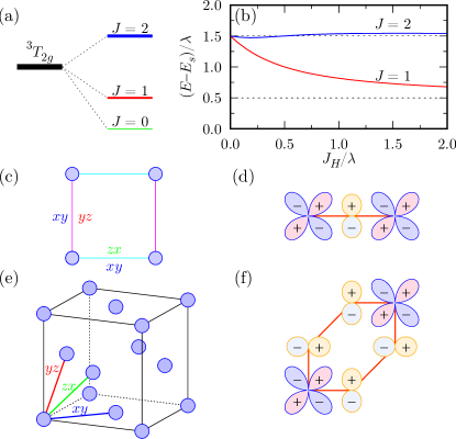
Figure 1: (Color online) (a) Energy splitting of the local multiplets due to the strong spin-orbit coupling. (b) Excitation energies from the $J=0$ multiplet for the microscopic model as a function of Hund’s coupling ($J_{H}$). $E_{s}$ refers to the ground state energy of the $J=0$ multiplet. Lattice structures of (c) corner-shared and (e) face-centered iridates, and their schematic orbital arrangements ((d) and (f)),which allow the hopping between adjacent iridiums. Orbital characters displayed in (c) and (e) represent dominant contributing orbitals between specific hopping directions.

II.2 Two Ir⁵⁺ sites

Now we study the magnetic exchange between nearest-neighboring Ir-sites due to electron hopping described by the following Hamiltonian:

$$H_{t}=\sum_{\alpha\beta\langle i,j\rangle}t_{\alpha\beta}c_{i\alpha}^{\dagger}c_{j\beta}+h.c..$$ (2)

In the following we will consider two types of lattices: layered perovskites and double perovskites. The dominant hoppings, found for these two lattices in the limit of linear combination of the atomic orbitals Slater , are illustrated in Fig. 1(d) and (f). In the layered perovskites the Ir-O-Ir geometry is $180^{\circ}$-bond formed by corner-shared octahedra as in Fig. 1(d). In this case the dominant hopping is between adjacent $xy$ orbitals and between $zx$ ($yz$) orbitals along the x-axis (y-axis). Its value is $-V_{pd\pi}^{2}/\Delta$, where $V_{pd\pi}$ and $\Delta$ are the $\pi$ bonding strength between $p$ and $d$ orbital, and the charge transfer energy of oxygens, respectively. In double perovskites the Ir geometry is face-centered system as in Fig. 1(f) and the dominant hopping is between $xy$ orbitals in the $xy$-plane. It can be expressed as $-V_{pd\pi}^{2}(V_{pp\sigma}-V_{pp\pi})/\Delta^{2}$, where $V_{pp\sigma}$ and $V_{pp\pi}$ are the $\sigma$ and $\pi$ bondings between $p$ orbitals. Although the hopping between $yz$ and $zx$ orbitals is also possible with the strength $-V_{pd\pi}^{2}V_{pp\pi}/\Delta^{2}$, it can be neglected in leading order, since $\left|V_{pp\pi}\right|\ll\left|V_{pp\sigma}\right|$. The obtained estimates for hopping are consistent with the results from density functional theory (DFT) calculations Dey2016 . For these reasons we restrict the consideration by two orbitals for the corner-shared system and by one orbit for the face-centered lattices with the nearest neighbors hopping $t$ ($t<0$) as it is illustrated in Fig. 1(c) and (e).

To proceed further we construct the Hilbert space for a two-site cluster that consists of all possible states whose configuration is $d^{4}$-$d^{4}$, $d^{3}$-$d^{5}$, or $d^{5}$-$d^{3}$. Then we find the eigenstate energies of the two-site cluster with help of the exact diagonalization (ED) method. Figure 2 presents the energy hierarchy and its partial density of states for $U=4.0$, $J_{H}=0.5$, $\lambda=0.4$, and $t=-0.4$ eV.

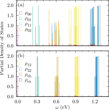
Figure 2: (Color online) Partial density of states of lowest eighty-one states of the two-site cluster for (a) corner-shared and (b) face-centered hopping when $U$=4.0, $J_{H}$=0.5, $\lambda=0.4$, and $t=-0.4$ eV. $\rho_{j_{1}j_{2}}$ represent the partial density of states in which $J=j_{1}$ is stabilized in one site and $J=j_{2}$ in another site. $\rho_{eh}$ and $\rho_{ex}$ refer to the partial density of states with $d^{3}$-$d^{5}$ or $d^{5}$-$d^{3}$ configuration, and remain states with $d^{4}$-$d^{4}$ configuration, respectively. The total density of nondegenerate state is one.

We introduce the partial density of states $\rho_{j_{1}j_{2}}$, in which local multiplet state is one out of $J=j_{1}$ and $j_{2}$ states, $\rho_{eh}$ to be the partial density of states of configuration is $d^{3}$-$d^{5}$ or $d^{5}$-$d^{3}$ (electron-hole (e-h) excitation states), and $\rho_{ex}$ to be the remaining multiplets. Since the e-h excitations appear above $U-3J_{H}+\lambda=2.9$ eV, multiplet states below 1.4 eV ($>1.5\lambda$) can be attributed to the $L=1,S=1$ manifold. We find that $\rho_{eh}$ and $\rho_{ex}$ in the region are always less than 10% in these parameters. This implies that the magnetic interactions between $L=1,~{}S=1$ multiplets are induced by the virtual hopping like superexchange interactions which give rise to the splitting of excitation multiplets. According to Fig. 2(a) and (b), the splittings in the corner-shared system are almost twice as large as those in the face-centered system. The corner-shared system has about $104$ meV of single-triplet ($\rho_{01}$) and $169$ meV of single-quintet ($\rho_{02}$) splitting, whereas the splittings in the face-centered system are $49$ meV and $71$ meV, correspondingly. This agrees with the expectation that the corner-shared system with two hopping channels has larger magnetic interactions than the face-centered system with one hopping channel.

III Effective low-lying spin-orbital excitations

III.1 Effective excitonic Hamiltonian

To derive an effective Hamiltonian for the interaction between different spin-orbital states, we define $E_{n}$ and $|\Psi_{n}\rangle$ be an eigenvalue and eigenstate of two-site cluster, respectively. In the limit of $U-3J_{H}>>2\lambda$, the effective interactions between $d^{4}$ multiplets ($L=1,S=1$) along the $\delta$-direction can be extracted from the two-site calculation as follows BHKim2012 ; Winter2016

$$H_{\delta} =\sum_{n=0}^{80}E_{n}\frac{\mathcal{P}_{LS}|\Psi_{n}\rangle\langle\Psi_{n}|\mathcal{P}_{LS}}{\langle\Psi_{n}|\mathcal{P}_{LS}^{2}|\Psi_{n}\rangle}$$

$$=\sum_{j_{1}j_{2}j_{1}^{\prime}j_{2}^{\prime}}\sum_{mnm^{\prime}n^{\prime}}E_{mnm^{\prime}n^{\prime}}^{j_{1}j_{2}j_{1}^{\prime}j_{2}^{\prime}}(\delta)|T_{m}^{j_{1}}T_{n}^{j_{2}}\rangle\langle T_{m^{\prime}}^{j_{1}^{\prime}}T_{n^{\prime}}^{j_{2}^{\prime}}|$$ (3)

where $T_{m}^{j}$ is the multiplet state with $J=j$ and $J_{z}=m$, $\mathcal{P}_{LS}$ is the projection operator into the $L=1,S=1$ manifold, and $|\Psi_{n}\rangle$ is one of lowest $81$ states. Since $J$-representation with $L=1$ and $S=1$ is very similar to a quantum dimer model for a spin-$1$ system, we can introduce the same bond-boson operators Sachdev1990 ; Brenig2001 (see appendix A) and derive the effective lattice Hamiltonian in terms of these bosons by considering all possible effective interactions incorporated in Eq. 3:

$$H_{\rm eff}=\sum_{i}\epsilon_{s}s_{i}^{\dagger}s_{i}+\sum_{i\alpha}\epsilon_{t}t^{\dagger}_{\alpha i}t_{\alpha i}+\sum_{i\mu}\epsilon_{q}q^{\dagger}_{\mu i}q_{\mu i}$$

$$~{}+\frac{1}{2}\sum_{i\delta\alpha\beta}\left([h_{\delta}^{11}]_{\alpha\beta}s_{i}^{\dagger}t_{\alpha i_{\delta}}^{\dagger}t_{\beta i}s_{i_{\delta}}+[d_{\delta}^{11}]_{\alpha\beta}t_{\beta i}^{\dagger}t_{\alpha i_{\delta}}^{\dagger}s_{i}s_{i_{\delta}}+h.c.\right)$$

$$~{}+\frac{1}{2}\sum_{i\delta\mu\nu}\left([h_{\delta}^{22}]_{\mu\nu}s_{i}^{\dagger}q_{\mu i_{\delta}}^{\dagger}q_{\nu i}s_{i_{\delta}}+[d_{\delta}^{22}]_{\mu\nu}q_{\nu i}^{\dagger}q_{\mu i_{\delta}}^{\dagger}s_{i}s_{i_{\delta}}+h.c.\right)$$

$$~{}+\frac{1}{2}\sum_{i\delta\alpha\mu}\left([h_{\delta}^{12}]_{\alpha\mu}s_{i}^{\dagger}t_{\alpha i_{\delta}}^{\dagger}q_{\mu i}s_{i_{\delta}}+[d_{\delta}^{12}]_{\alpha\mu}q_{\mu i}^{\dagger}t_{\alpha i_{\delta}}^{\dagger}s_{i}s_{i_{\delta}}+h.c.\right)$$

$$~{}+\frac{1}{2}\sum_{i\delta\mu\alpha}\left([h_{\delta}^{21}]_{\mu\alpha}s_{i}^{\dagger}q_{\mu i_{\delta}}^{\dagger}t_{\alpha i}s_{i_{\delta}}+[d_{\delta}^{21}]_{\mu\alpha}t_{\alpha i}^{\dagger}q_{\mu i_{\delta}}^{\dagger}s_{i}s_{i_{\delta}}+h.c.\right)$$

$$~{}+\cdots,$$ (4)

where $2\epsilon_{s}=E_{0000}^{0000}(\delta)$, $\epsilon_{t}~{}(\epsilon_{q})+\epsilon_{s}=E_{\alpha 0\alpha 0}^{1010}(\delta)~{}(E_{\mu 0\mu 0}^{2020}(\delta))$, $[h_{\delta}^{jj^{\prime}}]_{\tau\tau^{\prime}}=E_{0\tau\tau^{\prime}0}^{0jj^{\prime}0}(\delta)$, and $[d_{\delta}^{jj^{\prime}}]_{\tau\tau^{\prime}}=E_{\tau\tau^{\prime}00}^{jj^{\prime}00}(\delta)$. $i_{\delta}$ refers to the neighboring site of $i$-th site along the $\delta$ direction.

As it is shown in Appendix B, the interaction between triplet bosons ($\mathbf{h}_{\delta}^{11}$) is of the $XXZ$-type in both corner-shared and face-centered cases. Only the $Z$-direction varies depending on the bonding type. In corner-shared (face-centered) case, $Z$ will be $x$, $y$, and $z$ for the interaction along (in) the $x$- ($yz$-), $y$- ($zx$-), and $z$-axis ($xy$-plane), respectively. The different nature of the hopping, however, gives rise to a somewhat different characteristics in these two cases: a Heisenberg interaction is dominant in the corner-shared case, whereas the Ising interaction prevails in the face-center case. In addition, the interaction parameters between quintets ($\mathbf{h}_{\delta}^{22}$) show different behaviors according to the bonding nature. The interaction for the $Z^{2}$-type quintet in the corner-shared case gives minimum strength in contrast to the face-centered case where it gives maximum strength. Because the interaction parameters between triplets and quintets ($\mathbf{h}_{\delta}^{12}$ and $\mathbf{h}_{\delta}^{21}$) have non-zero elements as shown in table B3, the coupling between triplets and quintets emerges. $X$- and $Y$-type triplets can be coupled with $YZ$- and $ZX$-type quintets, respectively, when the displacement of neighboring sites is parallel to the $Z$-axis in the corner-shared case and the $XY$-plane in the face-center case.

III.2 Dispersion of spin-orbital excitations

Note that only singlet bosons condense in the case of weak inter-site interactions. To investigate the exciton dispersion and possible condensation in the triplet or quintet channel, we treat Hamiltonian Eq. 4 in the mean-field approximation (see the detail in appendix C) as following

$$H_{MF}\approx N\epsilon_{s}$$

$$~{}+\sum_{\mathbf{k}}\left[\bm{\psi}^{\dagger}_{\mathbf{k}}\mathbf{h}(\mathbf{k})\bm{\psi}_{\mathbf{k}}+\frac{1}{2}\left(\bm{\psi}^{\dagger}_{\mathbf{k}}\mathbf{d}(\mathbf{k})\bm{\psi}^{*}_{-\mathbf{k}}+h.c.\right)\right],$$ (5)

where $N$ is the system size. $\psi_{\mathbf{k}}^{\dagger}$ is the field operator of eight (triplet and quintet) excitonic boson operators with momentum $\mathbf{k}$. $\bm{\psi}^{*}_{-\mathbf{k}}$ is the transpose of $\bm{\psi}^{\dagger}_{-\mathbf{k}}$. Interaction matrices of triplet and quintet bosons $\mathbf{h}(\mathbf{k})$ and $\mathbf{d}(\mathbf{k})$ are given as

$$\mathbf{h}(\mathbf{k})=\begin{pmatrix}\epsilon_{t}-\epsilon_{s}&0\\ 0&\epsilon_{q}-\epsilon_{s}\end{pmatrix}+\sum_{\delta}\begin{pmatrix}\mathbf{h}_{\delta}^{11}&\mathbf{h}_{\delta}^{12}\\ \mathbf{h}_{\delta}^{21}&\mathbf{h}_{\delta}^{22}\end{pmatrix}e^{i\mathbf{k}\cdot\mathbf{r}_{\delta}},$$ (6a)

$$\mathbf{d}(\mathbf{k})=\sum_{\delta}\begin{pmatrix}\mathbf{d}_{\delta}^{11}&\mathbf{d}_{\delta}^{12}\\ \mathbf{d}_{\delta}^{21}&\mathbf{d}_{\delta}^{22}\end{pmatrix}e^{i\mathbf{k}\cdot\mathbf{r}_{\delta}}.$$ (6b)

The dispersions of the excitonic modes can be obtained by solving Eq. 5 with the help of the Bogoliubov transformation (see appendix D).

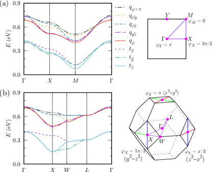
Figure 3: (Color online) Dispersions of eight excitonic modes (triplets and quintets) and Brillouin zone (BZ) of (a) the square lattice and (b) the face-centered cubic lattice when $U=4.0$, $J_{H}=0.5$, $\lambda=0.4$, and $t=-0.4$ eV. Red, green, and blue lines in (b), which are parallel to $x$-, $y$-, and $z$-axes, refer to the minimum line of $t_{x}$, $t_{y}$, and $t_{z}$, respectively, when all couplings between triplet and quintet bosons are neglected. Eight excitonic modes are well separated into three triplet dominant modes ($t_{\tilde{x}},t_{\tilde{y}},t_{\tilde{z}}$), three $t_{2g}$-type quintet dominant modes ($q_{\tilde{xy}},q_{\tilde{yz}},q_{\tilde{zx}}$), and two $e_{g}$-type quintet modes ($q_{\varphi},q_{\varphi+\pi}$). $\varphi$ varies depending on $\mathbf{k}$. $\varphi$’s at high symmetric points are presented in the BZ.

Figure 3 shows the dispersion of eight excitonic modes on square and fcc lattices with $U=4.0$, $J_{H}=0.5$, $\lambda=0.4$, and $t=-0.4$ eV. As shown in the parameter tables presented in Appendix B, all hopping matrices are well block diagonalized when eight bosons are divided into four subsectors like $\{t_{x},q_{yz}\}$, $\{t_{y},q_{zx}\}$, $\{t_{z},q_{xy}\}$, and $\{q_{z^{2}},q_{x^{2}-y^{2}}\}$. In addition, the energy splitting between triplet and quintet bosons ($\epsilon_{q}-\epsilon_{t}$) is considerably larger than their coupling strengths. Eight excitonic modes are well separated into three triplet dominant modes ($t_{\tilde{x}},t_{\tilde{y}},t_{\tilde{z}}$), three $t_{2g}$-type quintet dominant modes ($q_{\tilde{xy}},q_{\tilde{yz}},q_{\tilde{zx}}$), and two $e_{g}$-type quintet modes ($q_{\varphi},q_{\varphi+\pi}$).

On the square lattice, three triplet dominant modes show almost the same dispersions. From $\Gamma$ through $X$ to $M$ points, their energies monotonically decrease (see Fig. 3(a)). The $t_{\tilde{z}}$ mode has maximum (minimum) at the $\Gamma$ ($M$) point. Note that, the condensation of the $t_{\tilde{z}}$ bosons at $M$ point may be interpreted as the antiferomagnetic order with the $z$-component magnetic moment. The overall dispersions for five quintet dominant modes are quite similar. The $q_{\varphi_{\Gamma}+\pi}$ ($=q_{z^{2}}$) quintet has maximum value at $\Gamma$ and $q_{\varphi_{M}}$ ($=q_{z^{2}}$) has a minimum at $M$ with $\varphi_{\Gamma}=\pi$ and $\varphi_{M}=0$.

On the fcc lattice, triplet dominant modes have a maximum value at $\Gamma$, whereas both $t_{\tilde{y}}$ and $t_{\tilde{z}}$ reach the minimum at $X$-point. Their dispersions are consistent with those estimated in recent theoretical studies Pajskr2016 ; Chen2017 , in which triplet states are only considered, except for their minimum pattern. In contrast to our result, their minima appear on the $XW$ line away from $X$-point The discrepancy in the results stems from non-negligible coupling between triplet and quintet bosons, which was taken into account. Our calculation also exhibits lines of minima which are highlighted with red, green, and blue lines in Brillouin zone of Fig. 3(b) when the coupling between triplet and quintet bosons is turned off. In the presence of the coupling, dispersions of $t_{\tilde{y}}$ and $t_{\tilde{z}}$ modes at the $X$ point, to be shift down. Minimum of the dispersions appear only at the $X$ (also $Y$ and $Z$) point. Quintet dominant modes also show minimum values at $X$, $Y$, and $Z$ points. As shown in Fig. 3(b), $q_{\tilde{yz}}$ at $X$, $q_{\tilde{zx}}$ at $Y$, and $q_{\tilde{xy}}$ at $Z$ have minimum energy. Note that $\varphi_{\mathbf{k}}$’s at $X$, $Y$, and $Z$ are $\frac{5\pi}{3}$, $\frac{\pi}{3}$, and $\pi$, respectively, on the fcc lattice. The quintet $q_{\varphi_{X}}$ ($=q_{y^{2}-z^{2}}$) excitation can be the lowest mode when $U/t$ is small like Fig. 4(b).

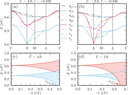
Figure 4: (Color online) Dispersion of eight excitonic modes of the face-centered-cubic lattice when (a) $U=4.0$ and $t=-0.459$ eV and (b) $U=2.6$ and $t=-0.346$ eV. Excitation ranges of triplet and quintet dominant modes when (c) $U=4.0$ and (d) $U=2.6$ eV. We set $J_{H}=0.5$ and $\lambda=0.4$ eV. Triplet and quintet condense when hopping strengths are larger than $-t_{c1}$ and $-t_{c2}$, respectively.

One observes that both triplet and quintet modes become more dispersive when the hopping amplitude increases. Eventually, one of modes will condense if the hopping strength exceeds a critical value which we label $t_{c1}$ for the triplet and $t_{c2}$ for the quintet. Because multiplet levels of triplets and quintets are about 0.31 and 0.62 eV, respectively, for $J_{H}=0.5$ and $\lambda=0.4$ eV, it seems likely that the triplet dominant modes always condenses first. For this reason only triplet bosons have been took into account to explore the magnetic excitation of $d^{4}$ systems in previous works. Our calculation, however, shows that such is not necessarily true for the fcc lattice. Figure 4(a) and (b) present dispersions of excitonic modes on the fcc lattice for two different sets of parameters. When $U=4.0$ and $t=-0.459$ eV, $t_{\tilde{y}}$ and $t_{\tilde{z}}$ modes are about to condense at the $X$ point. Quintet dominant modes are dispersive above $0.4$ eV. When $U=2.6$ and $t=-0.346$ eV, in contrast, minimum point of $q_{\varphi=5\pi/3}$ ($q_{y^{2}-z^{2}}$) mode is close to zero at the $X$ point even though spectra of triplet dominant modes are located above $0.1$ eV. Figure 4(c) and (d) give more detail how triplet and quintet dominant modes are extended as a function of hopping strength. For a not too large $U$ of $2.6$ eV, even quintets of which the local excitation energy is higher, soften very quickly with increasing hopping strength and condense first, in contrast to the situation for a larger $U$ of $4.0$ eV, in which they exhibit similar a softening tendency as triplets are not the first instability of the system.

IV Electronic excitation

To get the dispersion of spin-orbit excitons, we assume that the e-h excitations, which are described with the partial density of state $\rho_{\rm eh}$ for two-sites, appear in quite higher energy than spin-orbit excitons. It is valid for the two-sites model for the considered parameters, but it is not obvious for a lattice. When Coulomb repulsion is small enough in comparison to the hopping parameter, the dispersion of e-h excitations can overlap with spin-orbit excitons. Eventually, charge gap closes and insulator-metal transition (IMT) occurs. Then the effective spin-orbital excitonic description breaks down. Therefore, it is necessary to investigate the spectrum of e-h excitations as functions of both hopping and Coulomb interaction.

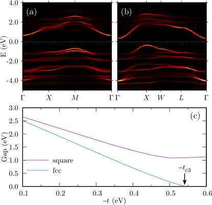
Figure 5: (Color online) Spectral functions of (a) square lattice and (b) face-centered-cubic lattice calculated by variational CPT with four-site cluster when $U=4.0$, $J_{H}=0.5$, $\lambda=0.4$, and $t=-0.4$ eV. (c) The insulating gap behavior as a function of the hopping strength $t$ when $U=4.0$, $J_{H}=0.5$, and $\lambda=0.4$ eV. When the hopping strength is larger than $-t_{c3}$, the insulating gap is closed and semimetallic phase is stabilized.

We adopt the CPT Senechal2002 with chemical potential optimization via the variational cluster approximation (VCA) Potthoff2003 . We calculate the cluster Green’s function $\mathbf{G}^{\prime}(z,\mu_{c})$ with the four-site cluster presented in inset of Fig. 1(c) and (e). The cluster chemical potential $\mu_{c}$ is determined so that the average number per site is four in the ground state. The lattice Green’s function $\mathbf{G}(z,\mathbf{K})$ can be obtained with $\mathbf{G}(z,\mathbf{K})^{-1}=\mathbf{G}^{\prime}(z,\mu)-(\mu-\mu_{c})\mathbf{V}(\mathbf{K})$, where $\mu$ is the lattice chemical potential and $\mathbf{V}(\mathbf{K})$ is the Fourier transformation of the intercluster hopping matrix at crystal momentum $\mathbf{K}$ of four-site supercell. $\mu$ is optimized at the extremum point of the grand functional $\Omega$ ($\frac{\partial\Omega}{\partial\mu}=0$) Dahnken2004 .

Figures 5(a) and (b) present spectral functions of square and fcc lattice when $U=4.0$, $J_{H}=0.5$, $\lambda=0.4$ and $t=-0.4$ eV. Both systems are located at the Mott insulating phase exhibiting an indirect gap. When hopping strength increases, however, the gap size decreases and IMT occurs at $t_{c3}$ point. Due to the large coordination number, the gap variation vs the hopping parameter on the fcc lattice is more sensitive than that on the square lattice. As shown in Fig. 5(c), the gap on the fcc lattice is closed even if the hopping strength is less than 0.6 eV when $U=4.0$, $J_{H}=0.5$, and $\lambda=0.4$ eV, whereas the gap is still finite on the square lattice. Overall electronic phases for various parameters are presented in Fig. 6. Gray area in Fig. 6 refers to expected metallic region.

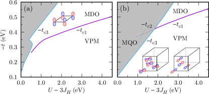
Figure 6: (Color online) Phase diagram of (a) square lattice and (b) face-centered-cubic lattice. Triplet and quintet condensations give rise to the magnetic transitions from the Van Vleck paramagnetic (VPM) phase to the magnetic dipole order (MDO), and from the VPM phase to the magnetic quadrupole order (MQO), respectively. Insets in (a) and (b) refer to the schematic diagrams of possible condensed bosons in ordered phases. Gray area refers to expected region of the metallic phase based on the variational CPT calculation. The MQO phase on the fcc lattice could hardly emerge because of advanced charge gap closure.

As shown in Fig. 6(a), the spectral function of the square lattice has an indirected gap determined at $\Gamma$ and $M$ points in Mott insulating phase far from the IMT boundary. However, its feature can vary in the vicinity of the IMT boundary when the hopping strength is large enough ($-t>0.35$ eV). As shown in Fig. 7(b), some portion of spectral weights transfers across the Fermi level around $\Gamma$ and $M$ points without the gap closure. Shape of spectral function changes from Fig. 5(a) to Fig. 7(b) when $U$ decreasing. However, the spectral weight transfer hardly occurs when the hopping strength is small ($-t<0.32$ eV). Overall shape of spectral function is almost robust until the gap is closed (see Fig. 7(a)). Consequently, the phase diagram of square lattice manifests different types of phase boundary depending on the hopping strength and shows the S-shape boundary around the intermediate hopping limit ($0.3<-t<0.4$ eV). On the fcc lattice, in contrast, the gap is always closed indirectly at $\Gamma$ and $X$ points for given parameter range. The spectral weight transfer across the Fermi level is hardly manifested. The phase boundary of IMT monotonically varies on the fcc lattice.

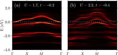
Figure 7: (Color online) Spectral functions of square lattice calculated by variational CPT when (a) $U=1.7$, $J_{H}=0.5$, $\lambda=0.4$, and $t=-0.2$ eV, and (b) $U=2.2$, $J_{H}=0.5$, $\lambda=0.4$, and $t=-0.4$ eV.

V Discussion

Singlet, triplet, and quintet condensations stabilize different types of ground states, namely, Van Vleck paramagnetic (VPM) for singlet, magnetic dipole order (MDO) for triplet, and magnetic quadrupole order (MQD) for quintet. The electronic and magnetic phase diagram as functions of $t$ and $U-3J_{H}$ is shown in Fig. 6(a) and (b) on the square and fcc lattices, respectively Hund . On the square lattice the charge gap is considerably larger than the excitonic gap in broad range of parameters. With increase of the hopping parameter, the magnetic ground state changes from VPM to MDO. The IMT may occur only in weak $U-3J_{H}$ ($<0.5$ eV) limit. Because $t_{\tilde{z}}$ triplet always condenses first, magnetic dipole moment is parallel to the $z$-axis with the ($\pi,\pi$) ordering. The situation on the fcc lattice is different. Because of large coordination number on the fcc lattice, the dispersion of e-h excitations is much larger than that on the square lattice. According to the magnetic phase diagram obtained from the effective spin-orbital Hamiltonian of two-site cluster, the instability towards condensation of quintet modes of $q_{y^{2}-z^{2}}$, $q_{z^{2}-x^{2}}$, and $q_{x^{2}-y^{2}}$ at $X$, $Y$, and $Z$ points, respectively, appears before that towards the condensation of triplet dominant modes in weak $U-3J_{H}$ ($<1.24$ eV) limit. It likely gives rise to the MQO like the schematic diagram at lower part of Fig. 6(b). Considering the electronic excitation, however, the MQO could hardly emerge on the fcc lattice. When $U-3J_{H}$ is less than about 1.82 eV, the VPM state can directly evolve to the metallic state without intermediate triplet or quintet condensations. Only in large $U-3J_{H}$ ($>1.82$ eV) limit, the MDO can take place before the IMT. In the phase, magnetic dipoles perpendicular to the $x$ ($y$ or $z$) axis are parallelly ordered when they are in same plane parallel to the $yz$ ($zx$ or $xy$) plane, whereas magnetic dipoles in adjacent planes are antiparallely ordered.

The experimentally relevant values of $U-3J_{H}$ in iridates are $0.4\sim 2.0$ eV Watanabe2010 ; Martins2011 ; Arita2012 ; BHKim2012 ; BHKim2014 . The value the hopping parameter, for instance Ba₂YIrO₆ for which band structure calculations find $t\sim 0.2$ eV Dey2016 , is still too low. The double-perovskite iridates are certainly paramagnetic insulators with spin-orbital singlet in nature. Their observed magnetic moment is surely attributed to not intrinsic but extrinsic origins. Moreover, the phase diagram of the fcc lattice implies that they barely exhibit any condensation of triplets or quintets but show a ferromagnetic or paramagnetic metallic phase in relevant parameter regime even enlarging the covalency and weakening the on-site coulomb interaction. In this regard materials, the typical situation for $4d$ transition metal elements with small coordination number like Ca₂RuO₄ is promising of the triplet condensation Akbari2014 ; Jain2017 .

VI Summary

We investigated the spin-orbital excitations of pentavalent iridium ions and their potential condensation on square and fcc lattices. Based on the effective singlet-triplet-quintet Hamiltonian, we have demonstrated that in both structures triplet condensation can occur when the hopping $t$ becomes larger, for still moderate values of the local electron-electron interaction $U$. We have also demonstrated that in the fcc structure,depending on the precise value of $U$, the condensation of quintets can be the leading instability. Even though its local multiplet energy is about double of triplets, a steep drop of the $q_{y^{2}-z^{2}}$ dispersion at $X$ point accelerates the softening. According to the variational CPT calculation, however, the electronic charge excitations are also strongly dispersive and the charge gap drops much faster than those of spin-orbital excitations despite the center of energy being even higher than those of both triplets and quintets. The magnetic transition driven by the condensation of spin-orbital excitations is thus unlike to occur in iridium double-perovskites such as Ba₂YIrO₆ because of strong SOC strength and moderate Coulomb interaction – $4d$ transition metal compounds can be more promising in this respect.

Appendix A Bond-boson representation

To describe lowest nine multiplets of $d^{4}$ in the strong SO limit, we introduce nine boson operators. Singlet boson ($J=0$) is

$$s^{\dagger}|vac\rangle=|T^{0}_{0}\rangle,$$ (7)

where $|vac\rangle$ is the vacuum state. Triplet bosons ($J=1$) are

$$t_{x}^{\dagger}|vac\rangle=-\frac{1}{\sqrt{2}}\left(|T^{1}_{-1}\rangle-|T^{1}_{1}\rangle\right)$$ (8)

$$t_{y}^{\dagger}|vac\rangle=-\frac{i}{\sqrt{2}}\left(T^{1}_{-1}\rangle+|T^{1}_{1}\rangle\right)$$ (9)

$$t_{z}^{\dagger}|vac\rangle=|T^{1}_{0}\rangle.$$ (10)

Quintet bosons ($J=2)$ are

$$q_{xy}^{\dagger}|vac\rangle=\frac{i}{\sqrt{2}}\left(|T^{2}_{-2}\rangle-|T^{2}_{2}\rangle\right)$$ (11)

$$q_{yz}^{\dagger}|vac\rangle=\frac{i}{\sqrt{2}}\left(|T^{2}_{-1}\rangle+|T^{2}_{1}\rangle\right)$$ (12)

$$q_{z^{2}}^{\dagger}|vac\rangle=|T^{2}_{0}\rangle$$ (13)

$$q_{zx}^{\dagger}|vac\rangle=\frac{1}{\sqrt{2}}\left(|T^{2}_{-1}\rangle-|T^{2}_{1}\rangle\right)$$ (14)

$$q_{x^{2}-y^{2}}^{\dagger}|vac\rangle=\frac{1}{\sqrt{2}}\left(|T^{2}_{-2}\rangle+|T^{2}_{2}\rangle\right).$$ (15)

In cubic or tetragonal system, it is more convenient to use new coordinate to describe quintet bosons given by $q_{xy}^{\dagger}$, $q_{yz}^{\dagger}$, $q_{zx}^{\dagger}$, $q_{\varphi}^{\dagger}$, and $q_{\varphi+\pi}^{\dagger}$ where

$$q_{\varphi}^{\dagger}=\cos\frac{\varphi}{2}q_{z^{2}}^{\dagger}-\sin\frac{\varphi}{2}q_{x^{2}-y^{2}}^{\dagger}.$$ (16)

$q_{\varphi}^{\dagger}$ can be $-q_{z^{2}}^{\dagger}$ for $\varphi=0$, $q_{x^{2}}^{\dagger}$ for $2\pi/3$, $q_{y^{2}}^{\dagger}$ for $4\pi/3$, $-q_{x^{2}-y^{2}}^{\dagger}$ for $\pi$, $q_{z^{2}-x^{2}}^{\dagger}$ for $\pi/3$, or $q_{y^{2}-z^{2}}^{\dagger}$ for $5\pi/3$.

Appendix B Interaction strength

Table B1: Non-zero interaction parameters between triplet bosons of the square and face-center-cubic (fcc) lattices when $U=4.0$, $J_{H}=0.5$, $\lambda=0.4$, and $t=-0.4$ eV. On the square (fcc) lattice, triplet indices $\{1,2,3\}$ represent $\{y,z,x\}$ along the $x$-axis ($yz$-plane), $\{z,x,y\}$ along the $y$-axis ($zx$-plane), or $\{x,y,z\}$ along the $z$-axis ($xy$-plane). Unit is eV.

	square	fcc		square	fcc
$[h_{\delta}^{11}]_{11}$	$0.0404$	$0.0040$	$[d_{\delta}^{11}]_{11}$	$0.0226$	$0.0041$
$[h_{\delta}^{11}]_{22}$	$0.0404$	$0.0040$	$[d_{\delta}^{11}]_{22}$	$0.0226$	$0.0041$
$[h_{\delta}^{11}]_{33}$	$0.0256$	$0.0231$	$[d_{\delta}^{11}]_{33}$	$0.0295$	$0.0248$

Table B2: Non-zero interaction parameters between quintet bosons of the square and face-center-cubic (fcc) lattices when $U=4.0$, $J_{H}=0.5$, $\lambda=0.4$, and $t=-0.4$ eV. On the square (fcc) lattice, quintet indices $\{4,5,6,7,8\}$ represent $\{yz,zx,x^{2},xy,y^{2}-z^{2}\}$ along the $x$-axis ($yz$-plane), $\{zx,xy,y^{2},yz,z^{2}-x^{2}\}$ along the $y$-axis ($zx$-plane), or $\{xy,yz,z^{2},zx,x^{2}-y^{2}\}$ along the $z$-axis ($xy$-plane). Unit is eV.

	square	fcc		square	fcc
$[h_{\delta}^{22}]_{44}$	$0.0530$	$0.0003$	$[d_{\delta}^{22}]_{44}$	$-0.0017$	$~{}\ 0.0006$
$[h_{\delta}^{22}]_{55}$	$0.0233$	$0.0153$	$[d_{\delta}^{22}]_{55}$	$-0.0294$	$-0.0188$
$[h_{\delta}^{22}]_{66}$	$0.0116$	$0.0186$	$[d_{\delta}^{22}]_{66}$	$~{}\ 0.0118$	$~{}\ 0.0250$
$[h_{\delta}^{22}]_{77}$	$0.0233$	$0.0153$	$[d_{\delta}^{22}]_{77}$	$-0.0294$	$-0.0188$
$[h_{\delta}^{22}]_{88}$	$0.0530$	$0.0003$	$[d_{\delta}^{22}]_{88}$	$-0.0017$	$~{}\ 0.0006$

Table B3: Non-zero interaction parameters between triplet and quintet bosons of the square and face-center-cubic (fcc) lattices when $U=4.0$, $J_{H}=0.5$, $\lambda=0.4$, and $t=-0.4$ eV. Indices 1 – 8 are same as those presented in table B1 and B2. Unit is eV.

	square	fcc		square	fcc
$[h_{\delta}^{12}]_{15}$	$~{}\ 0.0029i$	$-0.0088i$	$[d_{\delta}^{12}]_{15}$	$~{}\ 0.0035i$	$-0.0086i$
$[h_{\delta}^{12}]_{27}$	$-0.0029i$	$~{}\ 0.0088i$	$[d_{\delta}^{12}]_{27}$	$~{}\ 0.0035i$	$~{}\ 0.0086i$
$[h_{\delta}^{21}]_{51}$	$-0.0029i$	$~{}\ 0.0088i$	$[d_{\delta}^{21}]_{51}$	$-0.0035i$	$-0.0086i$
$[h_{\delta}^{21}]_{72}$	$~{}\ 0.0029i$	$-0.0088i$	$[d_{\delta}^{21}]_{72}$	$-0.0035i$	$~{}\ 0.0086i$

Appendix C Mean-field Hamiltonian

Because of the hardcore condition, only one boson will be occupied at each site with following relation

$$s_{i}^{\dagger}s_{i}+\sum_{\alpha}t_{\alpha i}^{\dagger}t_{\alpha i}+\sum_{\mu}q_{\mu i}^{\dagger}q_{\mu i}=1.$$ (17)

We have to solve following Hamiltonian:

$$H_{\rm eff}+\sum_{i}\lambda_{L}\Big{(}s_{i}^{\dagger}s_{i}+\sum_{\alpha}t_{\alpha i}^{\dagger}t_{\alpha i}+\sum_{\mu}q_{\mu i}^{\dagger}q_{\mu i}-1\Big{)}.$$ (18)

Provided that the ground state in which singlet bosons almost condense, we can treat $s_{i}(s_{i}^{\dagger})$ as scalar value $s$ according to the mean-field theory of Bose system. Let ${\bm{\psi}}_{i}^{\dagger}$ be the field operator of eight (triplet and quintet) excitonic bosons at the $i$-th site like

$${\bm{\psi}}_{i}^{\dagger}=\begin{pmatrix}t_{x,i}^{\dagger}&t_{y,i}^{\dagger}&t_{z,i}^{\dagger}&q_{xy,i}^{\dagger}&q_{yz,i}^{\dagger}&q_{zx,i}^{\dagger}&q_{z^{2},i}^{\dagger}&q_{x^{2}-y^{2},i}^{\dagger}\end{pmatrix}.$$ (19)

We can get following the mean-field Hamiltonian from Eq. 4:

$$H_{MF}^{s,\lambda_{L}}\approx N(\epsilon_{s}s^{2}+\lambda_{L}s^{2}-\lambda_{L})$$

$$~{}+\frac{1}{2}\sum_{i\delta}\left[\bm{\psi}_{i_{\delta}}^{\dagger}\mathbf{h}^{s,\lambda_{L}}_{\delta}\bm{\psi}_{i}+\bm{\psi}_{i_{\delta}}^{\dagger}\mathbf{d}_{\delta}^{s,\lambda_{L}}\bm{\psi}_{i}^{*}+h.c.\right]$$

$$~{}+\cdots,$$ (20)

where

$$\mathbf{h}^{s,\lambda_{L}}_{\delta}=\begin{pmatrix}\epsilon_{t}+\lambda_{L}&0\\ 0&\epsilon_{q}+\lambda_{L}\end{pmatrix}+s^{2}\begin{pmatrix}\mathbf{h}_{\delta}^{11}&\mathbf{h}_{\delta}^{12}\\ \mathbf{h}_{\delta}^{21}&\mathbf{h}_{\delta}^{22}\end{pmatrix},$$ (21a)

$$\mathbf{d}^{s,\lambda_{L}}_{\delta}=s^{2}\begin{pmatrix}\mathbf{d}_{\delta}^{11}&\mathbf{d}_{\delta}^{12}\\ \mathbf{d}_{\delta}^{21}&\mathbf{d}_{\delta}^{22}\end{pmatrix},$$ (21b)

and $N$ is total number of sites. $\bm{\psi}_{i}$ and $\bm{\psi}_{i}^{*}$ are the Hermitian conjugate and transpose of $\bm{\psi}_{i}^{\dagger}$ vector, respectively. Because the mean-field order parameter $s^{2}$ follows the saddle-conditions $\partial H_{MF}^{s,\lambda_{L}}/\partial s^{2}=0$, we can get $\lambda_{L}=-\epsilon_{s}$ and approximate $s^{2}=1$ when there is no condensation of a triplet or quintet boson. Finally, we can get following Hamiltonian:

$$H_{MF}\approx N\epsilon_{s}+$$

$$~{}+\sum_{\mathbf{k}}\left[\bm{\psi}^{\dagger}_{\mathbf{k}}\mathbf{h}(\mathbf{k})\bm{\psi}_{\mathbf{k}}+\frac{1}{2}\left(\bm{\psi}^{\dagger}_{\mathbf{k}}\mathbf{d}(\mathbf{k})\bm{\psi}^{*}_{-\mathbf{k}}+h.c.\right)\right]$$

$$~{}+\cdots$$ (22)

based on following Fourier transformation relations:

$$\bm{\psi}_{\mathbf{k}}=\frac{1}{\sqrt{N}}\sum_{i}\bm{\psi}_{i}e^{i\mathbf{k}\cdot\mathbf{r}_{i}},$$ (23a)

$$\mathbf{h}(\mathbf{k})=\begin{pmatrix}\epsilon_{t}-\epsilon_{s}&0\\ 0&\epsilon_{q}-\epsilon_{s}\end{pmatrix}+\sum_{\delta}\begin{pmatrix}\mathbf{h}_{\delta}^{11}&\mathbf{h}_{\delta}^{12}\\ \mathbf{h}_{\delta}^{21}&\mathbf{h}_{\delta}^{22}\end{pmatrix}e^{i\mathbf{k}\cdot\mathbf{r}_{\delta}},$$ (23b)

$$\mathbf{d}(\mathbf{k})=\sum_{\delta}\begin{pmatrix}\mathbf{d}_{\delta}^{11}&\mathbf{d}_{\delta}^{12}\\ \mathbf{d}_{\delta}^{21}&\mathbf{d}_{\delta}^{22}\end{pmatrix}e^{i\mathbf{k}\cdot\mathbf{r}_{\delta}},$$ (23c)

where $\mathbf{r}_{i}$ and $\mathbf{r}_{\delta}$ are the position vector of an $i$-site and the displacement vector between Ir’s along the $\delta$-direction, respectively.

Appendix D Bogoliubov transformation

Because of the matrix $\mathbf{d}(\mathbf{k})$, the field operator $\psi_{\mathbf{k}}^{\dagger}$ is coupled with $\psi_{-\mathbf{k}}^{\dagger}$. The mean-field Hamiltonian written in Eq. 5 can be extended as following

$$H_{MF}=N\epsilon_{s}-\frac{1}{2}\sum_{\mathbf{k}}\textrm{Tr}\left[\mathbf{h}(\mathbf{k})\right]$$

$$~{}+\frac{1}{2}\sum_{\mathbf{k}}\begin{pmatrix}\bm{\psi}_{\mathbf{k}}^{\dagger}&\bm{\psi}_{-\mathbf{k}}^{\intercal}\end{pmatrix}\begin{pmatrix}\mathbf{h}(\mathbf{k})&\mathbf{d}(\mathbf{k})\\ \mathbf{d}(\mathbf{k})^{\dagger}&\mathbf{h}(-\mathbf{k})^{\intercal}\end{pmatrix}\begin{pmatrix}\bm{\psi}_{\mathbf{k}}\\ \bm{\psi}^{*}_{-\mathbf{k}}\end{pmatrix},$$ (24)

where $\bm{\psi}_{-\mathbf{k}}^{\intercal}$ and $\mathbf{h}(-\mathbf{k})^{\intercal}$ are the transpose of $\bm{\psi}_{-\mathbf{k}}$ and $\mathbf{h}(-\mathbf{k})$, respectively. We can get the dynamic equation of motion of both $\bm{\psi}_{\mathbf{k}}$ and $\bm{\psi}_{-\mathbf{k}}^{\dagger}$ operators as following

$$i\hbar\partial_{t}\begin{pmatrix}\bm{\psi}_{\mathbf{k}}\\ \bm{\psi}_{-\mathbf{k}}^{*}\end{pmatrix}=\begin{pmatrix}\mathbf{h}(\mathbf{k})&\mathbf{\Delta}(\mathbf{k})\\ -\mathbf{\Delta}(\mathbf{k})^{\dagger}&-\mathbf{h}(-\mathbf{k})^{\intercal}\end{pmatrix}\begin{pmatrix}\bm{\psi}_{\mathbf{k}}\\ \bm{\psi}_{-\mathbf{k}}^{*}\end{pmatrix},$$ (25)

where $\mathbf{\Delta}(\mathbf{k})=\frac{1}{2}\left(\mathbf{d}(\mathbf{k})+\mathbf{d}(-\mathbf{k})^{\intercal}\right)$ Maldonado1993 . By solving the general eigenvalue problem of Eq. 25, we can get dispersions of excitonic normal modes.

Appendix E Magnetization

In terms of bond-boson operators, local magnetic moment along the $\gamma$-direction is expressed by following relation:

$$M_{\gamma}=A\left(t_{\gamma}^{\dagger}s+s^{\dagger}t_{\gamma}\right)+\tilde{g}J_{\gamma}\\ +\sum_{\alpha\beta}\left(m_{\alpha\beta}^{\gamma}t_{\alpha}^{\dagger}q_{\beta}+h.c.\right),$$ (26)

where $A$ is constant and $\tilde{g}$ is the $g$-tensor expressed into $\tilde{g}=g_{0}\oplus g_{1}\oplus g_{2}$ where $g_{j}$ is the $g$-tensor of a $J=j$ state. The matrix $\mathbf{m}^{z}$ has only three nonzero elements such as $m_{x,zx}^{z}=m_{y,yz}^{z}$ and $m_{z,z^{2}}^{z}$. When $J_{H}>>\lambda$, $A=\sqrt{6}$, $g_{0}=0$, and $g_{1}=g_{2}=1/2$. Besides, $A\approx 2.41$, $g_{0}=0$, $g_{1}=1/2$, and $g_{2}\approx 0.36$ when $J_{H}=0.5$ and $\lambda=0.4$ eV.

References

- (1) E. E. Rodriguez, F. Poineau, A. Llobet, B. J. Kennedy, M. Avdeev, G. J. Thorogood, M. L. Carter, R. Seshadri, D. J. Singh, and A. K. Cheetham, Phys. Rev. Lett. 106, 067201 (2011).
- (2) J. M. Longo, P. M. Raccah, and J. B. Goodenough, J. Appl. Phys. 39, 1327 (1968).
- (3) R. Lam, F. Wiss, and J. E. Greedan, J. Solid State Chem. 167, 182 (2002).
- (4) G. Cao, J. Bolivar, S. McCall, J. E. Crow, and R. P. Guertin, Phys. Rev. B 57, 11039(R) (1998).
- (5) Y. Singh and P. Gegenwart, Phys. Rev. B 82, 064412 (2010).
- (6) B. J. Kim, H. Jin, S. J. Moon, J.-Y. Kim, B.-G. Park, C. S. Leem, J. Yu, T. W. Noh, C. Kim, S.-J. Oh, J.-H. Park, V. Durairaj, G. Cao, and E. Rotenberg, Phys. Rev. Lett. 101, 076402 (2008).
- (7) B. J. Kim, H. Ohsumi, T. Komesu, S. Sakai, T. Morita, H. Takagi, and T. Arima, Science 323, 1329 (2009).
- (8) G. Jackeli and G. Khaliullin, Phys. Rev. Lett. 102, 017205 (2009).
- (9) J. Chaloupka, G. Jackeli, and G. Khaliullin, Phys. Rev. Lett. 105, 027204 (2010).
- (10) J. Kim, D. Casa, M. H. Upton, T. Gog, Y.-J. Kim, J. F. Mitchell, M. van Veenendaal, M. Daghofer, J. van den Brink, G. Khaliullin, and B. J. Kim, Phys. Rev. Lett. 108, 177003 (2012).
- (11) J. Kim, A. H. Said, D. Casa, M. H. Upton, T. Gog, M. Daghofer, G. Jackeli, J. van den Brink, G. Khaliullin, and B. J. Kim, Phys. Rev. Lett. 109, 157402 (2012).
- (12) B. H. Kim, G. Khaliullin, and B. I. Min, Phys. Rev. Lett. 109, 167205 (2012).
- (13) B. H. Kim, G. Khaliullin, and B. I. Min, Phys. Rev. B 89, 081109(R) (2014).
- (14) H. Okabe, M. Isobe, E. Takayama-Muromachi, A. Koda, S. Takeshita, M. Hiraishi, M. Miyazaki, R. Kadono, Y. Miyake, and J. Akimitsu, Phys. Rev. B 83, 155118 (2011).
- (15) S. Boseggia, R. Springell, H. C. Walker, H. M. Rønnow, C. R uegg, H. Okabe, M. Isobe, R. S. Perry, S. P. Collins, and D. F. McMorrow, Phys. Rev. Lett. 110, 117207 (2013).
- (16) S. Fujiyama, K. Ohashi, H. Ohsumi, K. Sugimoto, T. Takayama, T. Komesu, M. Takata, T. Arima, and H. Takagi, Phys. Rev. B 86, 174414 (2012).
- (17) J.-M. Carter and H.-Y. Kee, Phys. Rev. B 87, 014433 (2013).
- (18) Y. Singh, S. Manni, J. Reuther, T. Berlijn, R. Thomale, W. Ku, S. Trebst, and P. Gegenwart, Phys. Rev. Lett. 108, 127203 (2012).
- (19) S. Manni, S. Choi, I. I. Mazin, R. Coldea, M. Altmeyer, H. O. Jeschke, R. Valentí, and P. Gegenwart, Phys. Rev. B 89, 245113 (2014).
- (20) H. Gretarsson, J. P. Clancy, X. Liu, J. P. Hill, E. Bozin, Y. Singh, S. Manni, P. Gegenwart, J. Kim, A. H. Said, D. Casa, T. Gog, M. H. Upton, H.-S. Kim, J. Yu, V. M. Katukuri, L. Hozoi, J. van den Brink, and Y.-J. Kim, Phys. Rev. Lett. 110, 076402 (2013).
- (21) J. P. Clancy, H. Gretarsson, J. A. Sears, Y. Singh, S. Desgreniers, K. Mehlawat, S. Layek, G. K. Rozenberg, Y. Ding, M. H. Upton, D. Casa, N. Chen, J. Im, Y. Lee, R. Yadav, L. Hozoi, D. Efremov, J. van den Brink, and Y.-J. Kim, njp Quantum Materials 3, 35 (2018).
- (22) V. Hermann, M. Altmeyer, J. Ebad-Allah, F. Freund, A. Jesche, A. A. Tsirlin, M. Hanfland, P. Gegenwart, I. I. Mazin, D. I. Khomskii, R. Valentí, and C. A. Kuntscher, Phys. Rev. B 97, 020104 (2018).
- (23) S. Ducatman, I. Rousochatzakis, and N. B. Perkins, Phys. Rev. B 97, 125125 (2018).
- (24) M. Bremholm, S. Dutton, P. Stephens, and R. Cava, J. Solid State Chem. 184, 601 (2011).
- (25) L. Du, X. Sheng, H. Weng, and X. Dai, Europhys. Lett. 101, 27003 (2013).
- (26) G. Khaliullin, Phys. Rev. Lett. 111, 197201 (2013).
- (27) S. Sachdev and B. Keimer, Phys. Today 64, 29 (2011).
- (28) A. Akbari and G. Khaliullin, Phys. Rev. B 90, 035137 (2014).
- (29) G. Cao, T. F. Qi, L. Li, J. Terzic, S. J. Yuan, L. E. DeLong, G. Murthy, and R. K. Kaul, Phys. Rev. Lett. 112, 056402 (2014).
- (30) L. T. Corredor, G. Aslan-Cansever, M. Sturza, K. Manna, A. Maljuk, S. Gass, T. Dey, A. U. B. Wolter, O. Kataeva, A. Zimmermann, M. Geyer, C. G. F. Blum, S. Wurmehl, and B. Büchner, Phys. Rev. B 95, 064418 (2017).
- (31) T. Dey, A. Maljuk, D. V. Efremov, O. Kataeva, S. Gass, C. G. F. Blum, F. Steckel, D. Gruner, T. Ritschel, A. U. B. Wolter, J. Geck, C. Hess, K. Koepernik, J. van den Brink, S. Wurmehl, and B. Büchner, Phys. Rev. B 93, 014434 (2016).
- (32) S. Fuchs, T. Dey, G. Aslan-Cansever, A. Maljuk, S. Wurmehl, B. Büchner, and V. Kataev, Phys. Rev. Lett. 120, 237204 (2018).
- (33) Q. Chen, C. Svoboda, Q. Zheng, B. C. Sales, D. G. Mandrus, H. D. Zhou, J.-S. Zhou, D. McComb, M. Randeria, N. Trivedi, and J.-Q. Yan, Phys. Rev. B 96, 144423 (2017).
- (34) M. Kusch, V. M. Katukuri, N. A. Bogdanov, B. Büchner, T. Dey, D. V. Efremov, J. E. Hamann-Borrero, B. H. Kim, M. Krisch, A. Maljuk, M. M. Sala, S. Wurmehl, G. Aslan-Cansever, M. Sturza, L. Hozoi, J. van den Brink, and J. Geck, Phys. Rev. B 97, 064421 (2018).
- (35) K. Pajskr, P. Novák, V. Pokorný, J. Kolorenč, R. Arita, and J. Kuneš, Phys. Rev. B 93, 035129 (2016).
- (36) H. Gong, K. Kim, B. H. Kim, B. Kim, J. Kim, and B. Min, J. Magn. Magn. Mater. 454, 66 (2018).
- (37) J. C. Slater and G. F. Koster, Phys. Rev. 94, 1498 (1954).
- (38) S. M. Winter, Y. Li, H. O. Jeschke, and R. Valentí, Phys. Rev. B 93, 214431 (2016).
- (39) S. Sachdev and R. N. Bhatt, Phys. Rev. B 41, 9323 (1990).
- (40) W. Brenig and K. W. Becker, Phys. Rev. B 64, 214413 (2001).
- (41) D. Sénéchal, D. Perez, and D. Plouffe, Phys. Rev. B 66, 075129 (2002).
- (42) M. Potthoff, M. Aichhorn, and C. Dahnken, Phys. Rev. Lett. 91, 206402 (2003).
- (43) C. Dahnken, M. Aichhorn, W. Hanke, E. Arrigoni, and M. Potthoff, Phys. Rev. B 70, 245110 (2004).
- (44) The on-site repulsion energy in systems is determined by not but George2013 . For this reason, the phase diagram is given as a function of instead of .
- (45) H. Watanabe, T. Shirakawa, and S. Yunoki, Phys. Rev. Lett. 105, 216410 (2010).
- (46) C. Martins, M. Aichhorn, L. Vaugier, and S. Biermann, Phys. Rev. Lett. 107, 266404 (2011).
- (47) R. Arita, J. Kuneš, A. V. Kozhevnikov, A. G. Eguiluz, and M. Imada, Phys. Rev. Lett. 108, 086403 (2012).
- (48) A. Jain, M. A. Krautloher, J. Porras, G. H. Ryu, D. P. Chen, D. L. Abernathy, J. T. Park, A. Ivanov, J. Chaloupka, G. Khaliullin, B. Keimer, and B. J. Kim, Nat. Phys. , 633 (2017).
- (49) O. Maldonado, J. Math. Phys. 34, 5016 (1993).
- (50) A. Georges, L. de’ Medici, and J. Mravlje, Annu. Rev. Condens. Matter Phys. 4, 137 (2013).