Combining Distant and Direct Supervision for Neural Relation Extraction

Abstract

In relation extraction with distant supervision, noisy labels make it difficult to train quality models. Previous neural models addressed this problem using an attention mechanism that attends to sentences that are likely to express the relations. We improve such models by combining the distant supervision data with an additional directly-supervised data, which we use as supervision for the attention weights. We find that joint training on both types of supervision leads to a better model because it improves the model’s ability to identify noisy sentences. In addition, we find that sigmoidal attention weights with max pooling achieves better performance over the commonly used weighted average attention in this setup. Our proposed method achieves a new state-of-the-art result on the widely used FB-NYT dataset.

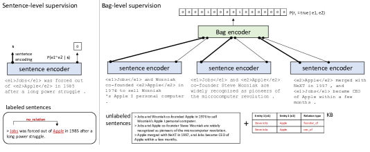
Figure 1: An overview of our approach for combining distant and direct supervision. The left side shows one sentence in the labeled data and how it is used to provide direct supervision for the sentence encoder. The right side shows snippets of the text corpus and the knowledge base, which are then combined to construct one training instance for the model, with a bag of three input sentences and two active relations: ‘founder_of’ and ‘ceo_of’.

1 Introduction

Early work in relation extraction from text used directly supervised methods, e.g., Bunescu and Mooney (2005), which motivated the development of relatively small datasets with sentence-level annotations such as ACE 2004/2005, BioInfer and SemEval 2010 Task 8. Recognizing the difficulty of annotating text with relations, especially when the number of relation types of interest is large, others (Mintz et al., 2009; Craven and Kumlien, 1999) introduced the distant supervision approach of relation extraction, where a knowledge base (KB) and a text corpus are used to automatically generate a large dataset of labeled bags of sentences (a set of sentences that might express the relation) which are then used to train a relation classifier. The large number of labeled instances produced with distant supervision make it a practical alternative to manual annotations.

However, distant supervision implicitly assumes that all the KB facts are mentioned in the text (at least one of the sentences in each bag expresses the relation) and that all relevant facts are in the KB (use entities that are not related in the KB as negative examples). These two assumptions are generally not true, which introduces many noisy examples in the training set. Although many methods have been proposed to deal with such noisy training data (e.g., Hoffmann et al., 2011; Surdeanu et al., 2012; Roth et al., 2013; Fan et al., 2014; Zeng et al., 2015; Jiang et al., 2016; Liu et al., 2017), a rather obvious approach has been understudied: combine distant supervision data with additional direct supervision. Intuitively, directly supervising the model can improve its performance by helping it identify which of the input sentences for a given pair of entities are more likely to express a relation.

A straightforward way to combine distant and direct supervision is to concatenate instances from both datasets into one large dataset. We show in Section 4.2 that this approach doesn’t help the model.  Pershina et al. (2014) also observed similar results; instead, they train a graphical model on the distantly supervised instances while using the directly labeled instances to supervise a subcomponent of the model. We discuss prior work in more detail in Section 5.

In our paper, we demonstrate a similar approach with neural networks. Specifically, our neural model attends over sentences to distinguish between sentences that are likely to express some relation between the entities and sentences that do not. We use the additional direct supervision to supervise these attention weights. We train this model jointly on both types of supervision in a multitask learning setup. In addition, we experimentally find that sigmoidal attention weights with max pooling achieves better performance in this model setup than the commonly used weighted average attention.

The contributions of this paper are as follows:

• We propose an effective neural network model for improving distant supervision by combining it with a directly supervised data in the form of sentence-level annotations. The model is trained jointly on both types of supervision in a multitask learning setup, where the direct supervision data is employed as supervision for attention weights.

• We show experimentally that our model setup benefits from sigmoidal attention weights with max pooling over the commonly used softmax-based weighted averaging attention.

• Our best model achieves a new state-of-the-art result on the FB-NYT dataset, previously used by Lin et al. (2016); Vashishth et al. (2018). Specifically, combining both forms of supervision achieves a 4.4% relative AUC increase than our baseline without the additional supervision.

The following section defines the notation we use, describes the problem and provides an overview of our approach.

2 Overview

Our goal is to predict which relation types are expressed between a pair of entities ($e_{1},e_{2}$), given all sentences in which both entities are mentioned in a large collection of unlabeled documents.

Following previous work on distant supervision, we use known tuples $(e_{1},r,e_{2})$ in a knowledge base $\cal{K}$ to automatically annotate sentences where both entities are mentioned with the relation type $r$. In particular, we group all sentences $s$ with one or more mentions of an entity pair $(e_{1},e_{2})$ into a bag of sentences $B_{e_{1},e_{2}}$, then automatically annotate this bag with the set of relation types $L^{\text{distant}}=\{r\in{\cal{R}}:(e_{1},r,e_{2})\in{\cal{K}}\}$, where $\cal{R}$ is the set of relations we are interested in. We use ‘positive instances’ to refer to cases where $|L|>0$, and ‘negative instances’ when $|L|=0$.

In this paper, we leverage an existing dataset of direct supervision for relations. Each direct supervision instance consists of a token sequence $s$ containing mentions of an entity pair $(e_{1},e_{2})$ and one relation type (or ‘no relation’). We do not require that the entities or relation types in the direct supervision annotations align with those in the KB. Furthermore, we replace the relation label associated with each sentence with a binary indicator of $1$ if the sentence expresses one of the relationships of interest and $0$ otherwise.

Figure 1 illustrates how we modify neural architectures commonly used in distant supervision, e.g., Lin et al. (2016); Liu et al. (2017) to effectively incorporate direct supervision. The model consists of two components: 1) A sentence encoder (displayed in blue) reads a sequence of tokens and their relative distances from $e_{1}$ and $e_{2}$, and outputs a vector $\mathbf{s}$ representing the sentence encoding, as well as $P(e_{1}\sim e_{2}\mid\mathbf{s})$ representing the probability that the two entities are related given this sentence. 2) The bag encoder (displayed in green) reads the encoding of each sentence in the bag for the pair $(e_{1},e_{2})$ and predicts $P(r=1\mid e_{1},e_{2}),\forall r\in{\cal{R}}$.

We combine both types of supervision in a multi-task learning setup by minimizing the weighted sum of the cross entropy losses for $P(e_{1}\sim e_{2}\mid\mathbf{s})$ and $P(r=1\mid e_{1},e_{2})$. By sharing the parameters of sentence encoders used to compute either loss, the sentence encoders become less susceptible to the noisy bag labels. The bag encoder also benefits from the direct supervision by using the supervised distribution $P(e_{1}\sim e_{2}\mid\mathbf{s})$ to decide the weight of each sentence in the bag.

3 Model

The model predicts a set of relation types ${L^{\text{pred}}\subset{\cal{R}}}$ given a pair of entities $e_{1},e_{2}$ and a bag of sentences $B_{e_{1},e_{2}}$. In this section, we first describe the sentence encoder part of the model (Figure 2, bottom), then describe the bag encoder (Figure 2, top), then we explain how the two types of supervision are jointly used for training the model end-to-end.

3.1 Sentence Encoder Architecture

Given a sequence of words $w_{1},\ldots,w_{|s|}$ in a sentence $s$, a sentence encoder translates this sequence into a fixed length vector $\mathbf{s}$.

Input Representation.

The input representation is illustrated graphically with a table at the bottom of Figure 2. We map word token $i$ in the sentence $w_{i}$ to a pre-trained word embedding vector $\mathbf{w}_{i}$. Another crucial input signal is the position of entity mentions in each sentence $s\in B_{e_{1},e_{2}}$. Following Zeng et al. (2014), we map the distance between each word in the sentence and the entity mentions to a small vector of learned parameters, namely $\mathbf{d}^{e_{1}}_{i}$ and $\mathbf{d}^{e_{2}}_{i}$.

We find that adding a dropout layer with a small probability ($p=0.1$) before the sentence encoder reduces overfitting and improves the results. To summarize, the input layer for a sentence $s$ is a sequence of vectors:

$$\mathbf{v}_{i}=[\mathbf{w}_{i};\mathbf{d}^{e_{1}}_{i};\mathbf{d}^{e_{2}}_{i}],\text{ for }i\in 1,\ldots,|s|$$

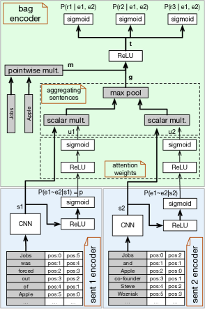
Figure 2: Blue box is the sentence encoder, it maps a sentence to a fixed length vector (CNN output) and the probability it expresses a relation between $e_{1}$ and $e_{2}$ (sigmoid output). Green box is the bag encoder, it takes encoded sentences and their weights and produces a fixed length vector (max pool output), concatenates it with entity embeddings (pointwise mult. output) then outputs a probability for each relation type $r$. White boxes contain parameters that the model learns while gray boxes do not have learnable parameters. Directly supervised annotations provide supervision for $P(e_{1}\sim e_{2}\mid\mathbf{s})$. Distantly supervised annotations provide supervision for $P(r=1\mid e_{1},e_{2})$.

Word Composition.

Word composition is illustrated with the block CNN in the bottom part of Figure 2, which represents a convolutional neural network (CNN) with multiple filter sizes. The outputs of the max pool operations for different filter sizes are concatenated then projected into a smaller vector using one feed forward linear layer.

Sentence encoding $\mathbf{s}$ is computed as follows:

$$\mathbf{c}_{x} =\text{ CNN}_{x}(\mathbf{v}_{1},\ldots,\mathbf{v}_{|s|}),\text{for }x\in\{2,3,4,5\}$$

$$\mathbf{s} =\mathbf{W}_{1}\>[\mathbf{c}_{2};\mathbf{c}_{3};\mathbf{c}_{4};\mathbf{c}_{5}]+\mathbf{b}_{1},$$

where $\text{CNN}_{x}$ is a standard convolutional neural network with filter size $x$, $\mathbf{W}_{1}$ and $\mathbf{b}_{1}$ are model parameters and $\mathbf{s}$ is the sentence encoding.

We feed the sentence encoding $s$ into a ReLU layer followed by a sigmoid layer with output size 1, representing $P(e_{1}\sim e_{2}\mid\mathbf{s})$, as illustrated in Figure 2 (bottom):

$$P(e_{1}\sim e_{2}\mid\mathbf{s}) =$$ (1)

$$p =\sigma(\mathbf{W}_{3}\text{ReLU}(\mathbf{W}_{2}\mathbf{s}+\mathbf{b}_{2})+\mathbf{b}_{3}),$$

where $\sigma$ is the sigmoid function and $\mathbf{W}_{2},\mathbf{b}_{2},\mathbf{W}_{3},\mathbf{b}_{3}$ are model parameters.

3.2 Bag Encoder Architecture

Given a bag $B_{e_{1},e_{2}}$ of $n\geq 1$ sentences, we compute their encodings $\mathbf{s}_{1},\ldots,\mathbf{s}_{n}$ as described earlier and feed them into the bag encoder, which combines the information in all of the sentence encodings and predicts the probability $P(r=1\mid e_{1},e_{2}),\forall r\in{\cal{R}}$. The bag encoder also incorporates the signal $p=P(e_{1}\sim e_{2}\mid\mathbf{s})$ from Equation 1 as an estimate of the degree to which sentence $s$ expresses “some” relation between $e_{1}$ and $e_{2}$.

Attention.

To aggregate the sentence encodings $\mathbf{s}_{1},\ldots,\mathbf{s}_{n}$ into a fixed length vector that captures the important features in the bag, we use attention. Attention has two steps: (1) computing weights for the sentences and (2) aggregating the weighted sentences. Weights can be uniform, or computed using a sigmoid or softmax. Weighted sentences can be aggregated using average pooling or max pooling. Prior work Jiang et al. (2016); Lin et al. (2016); Ji and Smith (2017) have explored some of these combinations but not all of them. In the ablation experiments, we try all combinations and we find that the (sigmoid, max pooling) attention gives the best result. We discuss the intuition behind this in Section 4.2. For the rest of this section, we will explain the architecture of our network assuming a (sigmoid, max pooling) attention.

Given the encoding $\mathbf{s}_{j}$ and an unnormalized weight $u_{j}$ for each sentence $s_{j}\in B_{e_{1},e_{2}}$, the bag encoding $\mathbf{g}$ is a vector with the same dimensionality as $\mathbf{s}_{j}$. With (sigmoid, max pooling) attention, each sentence vector is multiplied by the corresponding weight, then we do a “dimension-wise” max pooling (taking the maximum of each dimension across all sentences, not the other way around). The $k$-th element of the bag encoding $\mathbf{g}$ is computed as:

$$\mathbf{g}_{j}[k]=\text{max}_{j\in 1,\ldots,n}\{\mathbf{s}_{j}[k]\times\sigma(u_{j})\}.$$

As shown in Figure 2, we do not directly use the $p$ from Equation 1 as attention weights. Instead, we found it useful to feed it into more non-linearities. The unnormalized attention weight for $s_{j}$ is computed as:

$$u_{j}=\textbf{W}_{7}\>\text{ReLU}(\mathbf{W}_{6}\>p+\textbf{b}_{6})+\textbf{b}_{7}.$$

Entity Embeddings.

Following Ji et al. (2017), we use entity embeddings to improve our model of relations in the distant supervision setting, although our formulation is closer to that of Yang et al. (2015) who used point-wise multiplication of entity embeddings: ${\mathbf{m}=\mathbf{e}_{1}\odot\mathbf{e}_{2}},$ where $\odot$ is point-wise multiplication, and $\mathbf{e}_{1}$ and $\mathbf{e}_{2}$ are the embeddings of $e_{1}$ and $e_{2}$, respectively. In order to improve the coverage of entity embeddings, we use pretrained GloVe vectors  Pennington et al. (2014) (same embeddings used in the input layer). For entities with multiple words, like “Steve Jobs”, the vector for the entity is the average of the GloVe vectors of its individual words. If the entity is expressed differently across sentences, we average the vectors of the different mentions. As discussed in Section 4.2, this leads to big improvement in the results, and we believe there is still big room for improvement from having better representation for entities. We feed the output $\mathbf{m}$ as additional input to the last block of our model.

Output Layer.

The final step is to use the bag encoding $\mathbf{g}$ and the entity pair encoding $\mathbf{m}$ to predict a set of relations $L^{\text{pred}}$ which is a standard multilabel classification problem. We concatenate $\mathbf{g}$ and $\mathbf{m}$ and feed them into a feedforward layer with ReLU non-linearity, followed by a sigmoid layer with an output size of $|{\cal{R}}|$:

$$\mathbf{t} =\text{ReLU}(\mathbf{W}_{4}[\mathbf{g};\mathbf{m}]+\mathbf{b}_{4})$$

$$P(\mathbf{r}=1\mid e_{1},e_{2}) =\sigma(\mathbf{W}_{5}\mathbf{t}+\mathbf{b}_{5}),$$

where $\mathbf{r}$ is a vector of Bernoulli variables each of which corresponds to one of the relations in $\cal{R}$. This is the final output of the model.

3.3 Model Training

To train the model on the distant supervision data, we use binary cross-entropy loss between the model predictions and the labels obtained with distant supervision, i.e.,

$$\text{DistSupLoss}=\sum_{B_{e_{1},e_{2}}}-\log P(\mathbf{r}=\mathbf{r}^{\text{distant}}\mid e_{1},e_{2})$$

where $\mathbf{r}^{\text{distant}}[k]=1$ indicates that the tuple $(e_{1},r_{k},e_{2})$ is in the knowledge base.

In addition to the distant supervision, we want to improve the results by incorporating an additional direct supervision. A straightforward way to combine them is to create singleton bags for direct supervision labels, and add the bags to those obtained with distant supervision. However, results in Section 4.2 show that this approach does not improve the results. Instead, a better use of the direct supervision is to improve the model’s ability to predict the potential usefulness of a sentence. According to our analysis of baseline models, distinguishing between positive and negative examples is the real bottleneck in the task. Therefore, we use the direct supervision data to supervise $P(e_{1}\sim e_{2}\mid\mathbf{s})$. This supervision serves two purposes: it improves our encoding of each sentence, and improves the weights used by the attention to decide which sentences should contribute more to the bag encoding. It also has the side benefit of not requiring the same set of relation types as that of the distant supervision data, because we only care about if there exists some relevant relation or not between the entities.

We minimize log loss of gold labels in the direct supervision data ${\cal{D}}$ according to the model described in Equation 1:

$$\text{DirectSupLoss}=\sum_{s,l^{\text{gold}}\in{\cal{D}}}-\log P(l=l^{\text{gold}}\mid\mathbf{s})$$

where ${\cal{D}}$ is all the direct supervision data and all distantly-supervised negative examples.

We jointly train the model on both types of supervision. The model loss is a weighted sum of the direct supervision and distant supervision losses,

$$\text{loss}=\dfrac{1}{\lambda+1}\text{DistSupLoss}+\dfrac{\lambda}{\lambda+1}\text{DirectSupLoss}$$ (2)

where $\lambda$ is a parameter that controls the contribution of each loss, tuned on a validation set.

4 Experiments

4.1 Data and Setup

This section discusses datasets, metrics, configurations and the models we are comparing with.

Distant Supervision Dataset (DistSup).

The FB-NYT dataset introduced in Riedel et al. (2010) was generated by aligning Freebase facts with New York Times articles. The dataset has 52 relations with the most common being “location”, “nationality”, “capital”, “place_lived” and “neighborhood_of”. They used the articles of 2005 and 2006 for training, and 2007 for testing. Recent prior work (Lin et al., 2016; Liu et al., 2017; Huang and Wang, 2017) changed the original dataset. They used all articles for training except those from 2007, which they left for testing as in Riedel et al. (2010). We use the modified dataset which was made available by Lin et al. (2016). The table below shows the dataset size.

	Train	Test
Positive bags	16,625	1,950
Negative bags	236,811	94,917
Sentences	472,963	172,448

Direct Supervision Dataset (DirectSup).

Our direct supervision dataset was made available by Angeli et al. (2014) and it was collected in an active learning framework. The dataset consists of sentences annotated with entities and their relations. It has 22,766 positive examples for 41 relation types in addition to 11,049 negative examples. To use this dataset as supervision for $P(e_{1}\sim e_{2}\mid\mathbf{s})$, we replace the relation types of positive examples with $1$s and label negative examples with $0$s.

Metrics.

Prior work used precision-recall (PR) curves to show results on the FB-NYT dataset. In this multilabel classification setting, the PR curve is constructed using the model predictions on all entity pairs in the test set for all relation types sorted by the confidence scores from highest to lowest. Different thresholds correspond to different points on the PR curve. We use the area under the PR curve (AUC) for early stopping and hyperparameter tuning. Following previous work on this dataset, we only keep points on the PR curve with recall below $0.4$, focusing on the high-precision low-recall part of the PR curve. As a result, the largest possible value for AUC is $0.4$.

Configurations.

The FB-NYT dataset does not have a validation set for hyperparameter tuning and early stopping. Liu et al. (2017) use the test set for validation, Lin et al. (2016) use 3-fold cross validation, and Vashishth et al. (2018) split the training set into 80% training and 20% testing. In our experiments, we use 90% of the training set for training and keep the other 10% for validation. The main hyperparameter we tune is lambda (section 4.3).

The pre-trained word embeddings we use are 300-dimensional GloVe vectors, trained on 42B tokens. Since we do not update word embeddings while training the model, we define our vocabulary as any word which appears in the training, validation or test sets with frequency greater than two. When a word with a hyphen (e.g., ‘five-star’) is not in the GloVe vocabulary, we average the embeddings of its subcomponents. Otherwise, all OOV words are assigned the same random vector (normal with mean 0 and standard deviation 0.05).

Our model is implemented using PyTorch and AllenNLP (Gardner et al., 2017) and trained on machines with P100 GPUs. Each run takes five hours on average. We train for a maximum of 50 epoch, and use early stopping with patience $=3$. Each dataset is split into minibatches of size 32 and randomly shuffled before every epoch. We use the Adam optimizer with its default PyTorch parameters. We run every configuration with three random seeds and report the PR curve for the run with the best validation AUC. In the controlled experiments, we report the mean and standard deviation of the AUC across runs.

Compared Models.

Our best model (Section 3) is trained on the DistSup and DirectSup datasets in our multitask setup and it uses (sigmoid, max pooling) attention. Baseline is the same model described in Section 3 but trained only on the DistSup dataset and uses the more common (softmax, average pooling) attention. This baseline is our implementation of the PCNN+ATT model Lin et al. (2016) with two main differences; they use piecewise convolutional neural networks  (PCNNs Pennington et al., 2014) instead of CNNs, and we add entity embeddings before the output layer. We also compare our results to the state of the art model RESIDE (Vashishth et al., 2018), which uses graph convolution over dependency parse trees, OpenIE extractions and entity type constraints.

4.2 Main Results

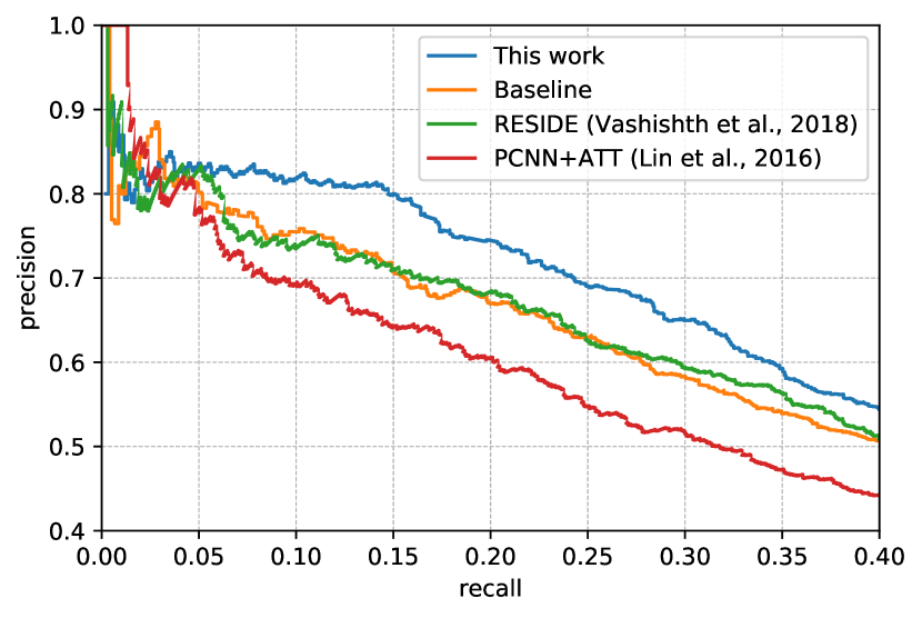
Model	AUC
PCNN+ATT (Lin et al., 2016)	0.247
RESIDE (Vashishth et al., 2018)	0.271
Our baseline	0.272±0.005
This work	0.283±0.007

Figure 3: Precision-recall curves and their AUC comparing our model with the baseline and existing models. Baseline is trained on DistSup and uses (softmax, average pooling) attention. Our best model is trained using multitask learning on DistSup and DirectSup and uses (sigmoid, max pooling) attention. Results of Lin et al. (2016) and Vashishth et al. (2018) are copied from their papers.

Figure 3 summarizes the main results of our experiments. First, we note that “our baseline” outperforms PCNN+ATT (Lin et al., 2016) despite using the same training data (DistSup) and the same form of attention (softmax, average pooling), which confirms that we are building on a strong baseline. The improved results in our baseline are due to using CNNs instead of PCNNs, and using entity embeddings.

A new state-of-the-art.

Adding DirectSup in our multitask learning setup and using (sigmoid, max pooling) attention gives us the best result, outperforming our baseline that doesn’t use either by 4.4% relative AUC increase, and achieves a new state-of-the-art result outperforming Vashishth et al. (2018).

We note that the improved results reported here conflate additional supervision and model improvements. Next, we report the results of controlled experiments to tease apart the contributions of different components.

pooling type	supervision signal	attention weight computation
		uniform	softmax	sigmoid
average pooling	DistSup	0.244$\pm$ 0.008	0.272$\pm$ 0.005	0.258$\pm$ 0.020
	DistSup + DirectSup	0.224$\pm$ 0.009	0.272$\pm$ 0.009	0.256$\pm$ 0.009
	MultiTask (our model)	0.220$\pm$ 0.012	0.262$\pm$ 0.014	0.258$\pm$ 0.015
max pooling	DistSup	0.277$\pm$ 0.009	0.278$\pm$ 0.001	0.274$\pm$ 0.004
	DistSup + DirectSup	0.269$\pm$ 0.003	0.269$\pm$ 0.005	0.277$\pm$ 0.012
	MultiTask (our model)	0.266$\pm$ 0.007	0.280$\pm$ 0.004	0.283$\pm$ 0.007

Table 1: Controlled experiments for a) how the supervised data is used in the model, b) which function is used to compute attention weights, c) how sentence embeddings are aggregated

Table 1 summarizes results of our controlled experiments showing the impact of how the training data is used, and the impact of different configurations of the attention (computing weights and aggregating vectors). The model can be trained on DistSup only, DistSup + DirectSup together as one dataset with DirectSup expressed as singleton bags, or DistSup + DirectSup in our multitask setup. Attention weights can be uniform, or computed using softmax or sigmoid. Sentence vectors are aggregated by weighting them then averaging (average pooling) or weighting them then taking the max of each dimension (max pooling). (Uniform weights, average pooling) and (softmax, average pooling) were used by Lin et al. (2016), (sigmoid, average pooling) was proposed by Ji and Smith (2017) but for a different task, and (uniform weights, max pooling) is used by Jiang et al. (2016). To the best of our knowledge, (softmax, max pooling) and (sigmoid, max pooling) have not been explored before.

Pooling type.

Results in Table 1 show that aggregating sentence vectors using max pooling generally works better than average pooling. This is because max pooling might be better at picking out useful features (dimensions) from each sentence.

Supervision signal.

The second dimension of comparison is the use of the supervision signal used to train the model. The table shows that training on DistSup + DirectSup, where the DirectSup dataset is simply used as additional bags, can hurt the performance. We hypothesize that this is because the DirectSup data change the distribution of relation types in the training set from the test set. However, using DirectSup as supervision for the attention weights in our multitask learning setup leads to considerable improvements (1% and 3% relative AUC increase using softmax and sigmoid respectively) because it leads to better attention weights and improves the model’s ability to filter noisy sentences.

Attention weight computation.

Finally, comparing uniform weights, softmax and sigmoid. We found the result to depend on the available level of supervision. With DistSup only, the results of all three are comparable with softmax being slightly better. However, when we have good attention weights (as provided by the multitask learning), softmax and sigmoid work better than uniform weights where sigmoid gives the best result with 6% relative AUC increase. Sigmoid works better than softmax, because softmax assumes that exactly one sentence is correct by forcing the probabilities to sum to 1. This assumption is not correct for this task, because zero or many sentences could potentially be relevant. On the other hand, sigmoidal attention weights does not make this assumption, which gives rise to more informative attention weights in cases where all sentences are not useful, or when multiple ones are. This makes the sigmoidal attention weights a better modeling for the problem (assuming reliable attention weights).

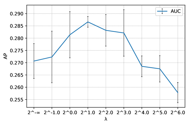
Figure 4: AUC at different $\lambda$. X-axis is in log-scale.

4.3 Selecting Lambda.

Although we did not spend much time tuning hyperparameters, we made sure to carefully tune $\lambda$ (Equation 2) which balances the contribution of the two losses of the multitask learning. Early experiments showed that DirectSupLoss is typically smaller than DistSupLoss, so we experimented with $\lambda\in\{0,0.5,1,2,4,8,16,32,64\}$. Figure 4 shows AUC results for different values of $\lambda$, where each point is the average of three runs. It is clear that picking the right value for $\lambda$ has a big impact on the final result.

4.4 Qualitative Analysis.

Baseline	This work	Sentences
0.00	0.029	You can line up along the route to cheer for the 32,000 riders, whose 42-mile trip will start in battery park and end with a festival at Fort Wadsworth on Staten Island .
0.00	0.026	Gateway is a home to the nation’s oldest continuing operating lighthouse, Sandy Hook lighthouse, built in 1764; Floyd Bennett field in Brooklyn, which was the city’s first municipal airfield; Fort Wadsworth on Staten Island, which predates the revolutionary war.
0.99	0.027	home energy smart fair, gateway national recreation area, Fort Wadsworth visitor center, bay street and school road, Staten Island.

Table 2: Weights assigned to sentences by our baseline and our best model. The baseline incorrectly predicts “no_relation”, while our best model correctly predicts “neighbourhood_of” for this bag.

An example of a positive bag is shown in Table 2. Our best model (Multitask, sigmoid, max pooling) assigns the most weight to the first sentence while the baseline (DistSup, softmax, average pooling) assigns the most weight to the last sentence (which is less informative for the relation between the two entities). Also, the baseline does not use the other two sentences because their weights are dominated by the last one.

5 Related Work

Distant Supervision.

The term ‘distant supervision’ was coined by Mintz et al. (2009) who used relation instances in a KB to identify sentences in a text corpus where two related entities are mentioned, then developed a classifier to predict the relation. Researchers have since extended this approach further (e.g., Takamatsu et al., 2012; Min et al., 2013; Riedel et al., 2013; Koch et al., 2014).

A key source of noise in distant supervision is that sentences may mention two related entities without expressing the relation between them. Hoffmann et al. (2011) used multi-instance learning to address this problem by developing a graphical model for each entity pair which includes a latent variable for each sentence to explicitly indicate the relation expressed by that sentence, if any. Our model can be viewed as an extension of Hoffmann et al. (2011) where the sentence-bound latent variables can also be directly supervised in some of the training examples.

Neural Models for Distant Supervision.

More recently, neural models have been effectively used to model textual relations (e.g., Hashimoto et al., 2013; Zeng et al., 2014; Nguyen and Grishman, 2015). Focusing on distantly supervised models, Zeng et al. (2015) proposed a neural implementation of multi-instance learning to leverage multiple sentences which mention an entity pair in distantly supervised relation extraction. However, their model picks only one sentence to represent an entity pair, which wastes the information in the neglected sentences. Jiang et al. (2016) addresses this limitation by max pooling the vector encodings of all input sentences for a given entity pair. Lin et al. (2016) independently proposed to use attention to address the same limitation, and Du et al. (2018) improved by using multilevel self-attention. To account for the noise in distant supervision labels, Liu et al. (2017); Luo et al. (2017); Wang et al. (2018) suggested different ways of using “soft labels” that do not necessarily agree with the distant supervision labels. Ye et al. (2017) proposed a method for leveraging dependencies between different relations in a pairwise ranking framework, while Han et al. (2018) arranged the relation types in a hierarchy aiming for better generalization for relations that do not have enough training data. To improve using additional resources, Vashishth et al. (2018) used graph convolution over dependency parse, OpenIE extractions and entity type constraints, and Liu et al. (2018) used parse trees to prune irrelevant information from the sentences.

Combining Direct and Distant Supervision.

Despite the substantial amount of work on both directly and distantly supervised relation extraction, the question of how to combine both signals has not received the same attention.  Pershina et al. (2014) trained MIML-RE from  (Surdeanu et al., 2012) on both types of supervision by locking the latent variables on the sentences to the supervised labels. Angeli et al. (2014) and Liu et al. (2016) presented active learning models that select sentences to annotate and incorporate in the same manner.  Pershina et al. (2014) and Liu et al. (2016) also tried simple baseline of including the labeled sentences as singleton bags.  Pershina et al. (2014) did not find this beneficial, which agrees with our results in Section 4.2, while Liu et al. (2016) found the addition of singleton bags to work well.

Our work is addressing the same problem, but combining both signals in a state-of-the-art neural network model, and we do not require the two datasets to have the same set of relation types.

6 Conclusion

We improve neural network models for relation extraction by combining distant and direct supervision data. Our network uses attention to attend to relevant sentences, and we use the direct supervision to improve attention weights, thus improving the model’s ability to find sentences that are likely to express a relation. We also found that sigmoidal attention weights with max pooling achieves better performance than the commonly used weighted average attention. Our model combining both forms of supervision achieves a new state-of-the-art result on the FB-NYT dataset with a 4.4% relative AUC increase than our baseline without the additional supervision.

References

- Angeli et al. (2014) Gabor Angeli, Julie Tibshirani, Jean Wu, and Christopher D Manning. 2014. Combining distant and partial supervision for relation extraction. In EMNLP.
- Bunescu and Mooney (2005) Razvan C. Bunescu and Raymond J. Mooney. 2005. A shortest path dependency kernel for relation extraction. In HLT/EMNLP.
- Craven and Kumlien (1999) Mark Craven and Johan Kumlien. 1999. Constructing biological knowledge bases by extracting information from text sources. In ISMB.
- Du et al. (2018) Jinhua Du, Jingguang Han, Andy Way, and Dadong Wan. 2018. Multi-level structured self-attentions for distantly supervised relation extraction. In EMNLP.
- Fan et al. (2014) Miao Fan, Deli Zhao, Qiang Zhou, Zhiyuan Liu, Thomas Fang Zheng, and Edward Y. Chang. 2014. Distant supervision for relation extraction with matrix completion. In ACL.
- Gardner et al. (2017) Matt Gardner, Joel Grus, Mark Neumann, Oyvind Tafjord, Pradeep Dasigi, Nelson F. Liu, Matthew Peters, Michael Schmitz, and Luke S. Zettlemoyer. 2017. Allennlp: A deep semantic natural language processing platform.
- Han et al. (2018) Xu Han, Pengfei Yu, Zhiyuan Liu, Maosong Sun, and Peng Li. 2018. Hierarchical relation extraction with coarse-to-fine grained attention. In EMNLP.
- Hashimoto et al. (2013) Kazuma Hashimoto, Makoto Miwa, Yoshimasa Tsuruoka, and Takashi Chikayama. 2013. Simple customization of recursive neural networks for semantic relation classification. In EMNLP.
- Hoffmann et al. (2011) Raphael Hoffmann, Congle Zhang, Xiao Ling, Luke S. Zettlemoyer, and Daniel S. Weld. 2011. Knowledge-based weak supervision for information extraction of overlapping relations. In ACL.
- Huang and Wang (2017) Yi Yao Huang and William Yang Wang. 2017. Deep residual learning for weakly-supervised relation extraction. In EMNLP.
- Ji et al. (2017) Guoliang Ji, Kang Liu, Shizhu He, and Jun Zhao. 2017. Distant supervision for relation extraction with sentence-level attention and entity descriptions. In AAAI.
- Ji and Smith (2017) Yangfeng Ji and Noah A. Smith. 2017. Neural discourse structure for text categorization. In ACL.
- Jiang et al. (2016) Xiaotian Jiang, Quan Wang, Peng Li, and Bin Wang. 2016. Relation extraction with multi-instance multi-label convolutional neural networks. In COLING.
- Koch et al. (2014) Mitchell Koch, John Gilmer, Stephen Soderland, and Daniel S. Weld. 2014. Type-aware distantly supervised relation extraction with linked arguments. In EMNLP.
- Lin et al. (2016) Yankai Lin, Shiqi Shen, Zhiyuan Liu, Huanbo Luan, and Maosong Sun. 2016. Neural relation extraction with selective attention over instances. In ACL.
- Liu et al. (2016) Angli Liu, Stephen Soderland, Jonathan Bragg, Christopher H. Lin, Xiao Ling, and Daniel S. Weld. 2016. Effective crowd annotation for relation extraction. In NAACL.
- Liu et al. (2017) Tian Yu Liu, Kexiang Wang, Baobao Chang, and Zhifang Sui. 2017. A soft-label method for noise-tolerant distantly supervised relation extraction. In EMNLP.
- Liu et al. (2018) Tianyi Liu, Xinsong Zhang, Wanhao Zhou, and Weijia Jia. 2018. Neural relation extraction via inner-sentence noise reduction and transfer learning. In EMNLP.
- Luo et al. (2017) Bingfeng Luo, Yansong Feng, Zheng Wang, Zhanxing Zhu, Songfang Huang, Rui Yan, and Dongyan Zhao. 2017. Learning with noise: Enhance distantly supervised relation extraction with dynamic transition matrix. In ACL.
- Min et al. (2013) Bonan Min, Ralph Grishman, Li Wan, Chang Wang, and David Gondek. 2013. Distant supervision for relation extraction with an incomplete knowledge base. In HLT-NAACL.
- Mintz et al. (2009) Mike Mintz, Steven Bills, Rion Snow, and Daniel Jurafsky. 2009. Distant supervision for relation extraction without labeled data. In ACL.
- Nguyen and Grishman (2015) Thien Huu Nguyen and Ralph Grishman. 2015. Relation extraction: Perspective from convolutional neural networks. In VS@HLT-NAACL.
- Pennington et al. (2014) Jeffrey Pennington, Richard Socher, and Christopher D. Manning. 2014. Glove: Global vectors for word representation. In EMNLP.
- Pershina et al. (2014) Maria Pershina, Bonan Min, Wei Xu, and Ralph Grishman. 2014. Infusion of labeled data into distant supervision for relation extraction. In ACL.
- Rei and Søgaard (2018) Marek Rei and Anders Søgaard. 2018. Zero-shot sequence labeling: Transferring knowledge from sentences to tokens. In NAACL-HLT.
- Riedel et al. (2010) Sebastian Riedel, Limin Yao, and Andrew D McCallum. 2010. Modeling relations and their mentions without labeled text. In ECML/PKDD.
- Riedel et al. (2013) Sebastian Riedel, Limin Yao, Andrew D McCallum, and Benjamin M. Marlin. 2013. Relation extraction with matrix factorization and universal schemas. In HLT-NAACL.
- Roth et al. (2013) Benjamin Roth, Tassilo Barth, Michael Wiegand, and Dietrich Klakow. 2013. A survey of noise reduction methods for distant supervision. In AKBC@CIKM.
- Surdeanu et al. (2012) Mihai Surdeanu, Julie Tibshirani, Ramesh Nallapati, and Christopher D. Manning. 2012. Multi-instance multi-label learning for relation extraction. In EMNLP-CoNLL.
- Takamatsu et al. (2012) Shingo Takamatsu, Issei Sato, and Hiroshi Nakagawa. 2012. Reducing wrong labels in distant supervision for relation extraction. In ACL.
- Vashishth et al. (2018) Shikhar Vashishth, Rishabh Joshi, Sai Suman Prayaga, Chiranjib Bhattacharyya, and Partha Talukdar. 2018. Reside: Improving distantly-supervised neural relation extraction using side information. In EMNLP.
- Wang et al. (2018) Guanying Wang, Wen Zhang, Ruoxu Wang, Yalin Zhou, Xi Chen, Wei Zhang, Hai Zhu, and Huajun Chen. 2018. Label-free distant supervision for relation extraction via knowledge graph embedding. In EMNLP.
- Yang et al. (2015) Bishan Yang, Wen tau Yih, Xiaodong He, Jianfeng Gao, and Li Deng. 2015. Embedding entities and relations for learning and inference in knowledge bases. In ICLR.
- Ye et al. (2017) Hai Ye, Wen-Han Chao, Zhunchen Luo, and Zhoujun Li. 2017. Jointly extracting relations with class ties via effective deep ranking. In ACL.
- Zeng et al. (2015) Daojian Zeng, Kang Liu, Yubo Chen, and Jun Zhao. 2015. Distant supervision for relation extraction via piecewise convolutional neural networks. In EMNLP.
- Zeng et al. (2014) Daojian Zeng, Kang Liu, Siwei Lai, Guangyou Zhou, and Jun Zhao. 2014. Relation classification via convolutional deep neural network. In COLING.