Binary planet formation by gas-assisted encounters of planetary embryos

Abstract

We present radiation hydrodynamic simulations in which binary planets form by close encounters in a system of several super-Earth embryos. The embryos are embedded in a protoplanetary disk consisting of gas and pebbles and evolve in a region where the disk structure supports convergent migration due to Type I torques. As the embryos accrete pebbles, they become heated and thus affected by the thermal torque (Benítez-Llambay et al., 2015) and the hot-trail effect (Chrenko et al., 2017) which excites orbital eccentricities. Motivated by findings of Eklund & Masset (2017), we assume the hot-trail effect operates also vertically and reduces the efficiency of inclination damping. Non-zero inclinations allow the embryos to become closely packed and also vertically stirred within the convergence zone. Subsequently, close encounters of two embryos assisted by the disk gravity can form transient binary planets which quickly dissolve. Binary planets with a longer lifetime $\sim$$10^{4}\,\mathrm{yr}$ form in 3-body interactions of a transient pair with one of the remaining embryos. The separation of binary components generally decreases in subsequent encounters and due to pebble accretion until the binary merges, forming a giant planet core. We provide an order-of-magnitude estimate of the expected occurrence rate of binary planets, yielding one binary planet per $\simeq$$2$–$5\times 10^{4}$ planetary systems. Therefore, although rare, the binary planets may exist in exoplanetary systems and they should be systematically searched for.

1 Introduction

Several classes of celestial objects are known to exist in binary configurations (e.g. minor solar-system bodies, dwarf planets, stars, etc.) – as two bodies orbiting their barycenter which is located exterior to their physical radii. The existence of binaries is an important observational constraint because a successful population synthesis model for a given class of objects must be able to explain how binaries form, how frequent they are, how they dynamically evolve and affect their neighborhood.

Concerning binary objects within the scope of planetary sciences, the richest sample is in the population of minor solar-system bodies. Examples can be found among the near-Earth objects (NEOs; e.g. Margot et al., 2002; Pravec et al., 2006; Scheeres et al., 2006), main-belt asteroids (MBAs; e.g. Marchis et al., 2008; Pravec et al., 2012), Jovian Trojans (e.g. Marchis et al., 2006; Sonnett et al., 2015) and surprisingly frequently among the Kuiper-belt objects (KBOs; e.g. Veillet et al., 2002; Brown et al., 2006; Richardson & Walsh, 2006; Noll et al., 2008). Formation of binary minor bodies took place during various epochs of the Solar System. Some binary asteroids originate in recent breakup events (Walsh et al., 2008), whereas the binary KBOs were probably established early, during the planetesimal formation (Goldreich et al., 2002; Nesvorný et al., 2010; Fraser et al., 2017) more than four billion years ago.

For large bodies, the number of binary configurations suddenly drops almost to zero. As for the known and confirmed objects, only Pluto and Charon can be considered a binary (Christy & Harrington, 1978; Walker, 1980; Lee & Peale, 2006; Brozović et al., 2015), likely of an impact origin (Canup, 2011; McKinnon et al., 2017). Since Pluto and Charon were classified as dwarf planets, the conclusion stands that planets in binary configurations have not yet been discovered.

Given that more than 3700 exoplanets have been confirmed up to date, the paucity of binary planets is a well-established characteristic of the dataset. However, its implications for our understanding of planet formation are unclear and maybe even underrated at present. Are the binary planets scarce and are we only unable to discover them with current methods? Or is their non-existence a universal feature shared by all planetary systems throughout the Galaxy?

To start addressing these questions, this paper discusses formation of binary planets by 2- and 3-body encounters of planetary embryos in protoplanetary disks, during the phase when the gas is still abundant and the embryos still grow by pebble accretion (Ormel & Klahr, 2010; Lambrechts & Johansen, 2012). We advocate that suitable conditions to form binary planets are achieved when orbital eccentricities and inclinations or embryos are excited by thermal torques related to accretion heating (Chrenko et al., 2017; Eklund & Masset, 2017). Our model utilizes radiation hydrodynamics (RHD) to account for these effects.

Although the results of this paper are preliminary in many aspects, they demonstrate that binary planets can exist and it may be only a matter of time (or method advancements) before an object like this is discovered in one of the exoplanet search campaigns. To motivate future observations and data mining, we emphasize that promising methods for detections of exomoons have been developed and applied in recent years. These include, for example, the transit timing variations (TTVs; Simon et al., 2007) and transit duration variations (TDVs; Kipping, 2009), their Bayesian analysis in the framework of direct star-planet-moon modeling and fitting (Kipping et al., 2012), photometric analysis of phase-folded light curves using the scatter peak (SP) method (Simon et al., 2012) or the orbital sampling effect (OSE; Heller, 2014; Hippke, 2015), microlensing events (Han, 2008; Liebig & Wambsganss, 2010; Bennett et al., 2014), or asymmetric light curves due to plasma tori of hypothetic volcanic moons (Ben-Jaffel & Ballester, 2014).

Indeed, Kepler-1625 b-i has been recently identified as an exomoon candidate (Heller, 2018; Teachey et al., 2018) and is waiting for a conclusive confirmation. Moreover, Lewis et al. (2015) discusses that the CoRoT target SRc01 E2 1066 can be explained as a binary gas-giant planet, although the signal can also correspond to a single planet transiting a star spot (Erikson et al., 2012). Therefore, methods similar to those listed above could be applicable when searching for binary planets.

Our paper is organized as follows. In Section 2, we outline our RHD model. Section 3 describes our nominal simulation with the binary planet formation. Planetary encounters are analyzed, as well as the influence of the gas disk. Subsequently, we test the stability of binary planets in several simplified models (without neighboring embryos; without the disk; etc.). We also study binary planet formation in a set of four additional simulations to verify the relevance of the process. In Section 4, we estimate the expected occurrence rate of binary planets in the exoplanetary population and we also discuss a possible role of binary planets in planetary sciences. Section 5 is devoted to conclusions.

1.1 Definitions

To avoid confusion, let us list several definitions which we use throughout the rest of the paper.

• Binary is a shortcut for a binary planet, not to be mistaken with binary stars etc.

• Transient (also transient binary or transient pair) is a binary which forms by 2-body encounters of planetary embryos (e.g. Astakhov et al., 2005), in our case with the assistance of the disk gravity as we shall demonstrate later. We choose the name transient because we find the typical lifetime of these binaries to be of the order of one stellarcentric orbital period.

• Hardening (e.g. Hills, 1975) is a process during which the orbital energy of a binary configuration is dissipated and the separation of binary components decreases.

• Stability of a binary planet is considered if it can survive at least more than one stellarcentric orbital period, which is usual after hardening. In principle, such a binary can be observed. We characterize the stability by means of the lifetime on which the binary components remain gravitationally bound.

• Encounter refers to a close encounter of two and more planetary embryos (single or binary), when they enter one another’s Hill sphere.

• Merger refers to a physical collision of two embryos. In our approximation, we replace the colliding embryos by a single object, assuming perfect merger (mass and momentum conservation).

• We denote orbital elements in the stellarcentric frame with a subscript ‘s’ to distinguish them from the orbital elements of one binary component with respect to another (e.g. $a_{\mathrm{s}}$ is the stellarcentric semimajor axis but $a$ is the semimajor axis of the binary configuration).

2 Radiation hydrodynamic model

2.1 General overview

The individual constituents of our model are as follows. First, we consider radiation transfer which is essential to properly reproduce the disk structure (Bitsch et al., 2013) and to account for all components of the Type I torque acting on low-mass planets (e.g. Baruteau & Masset, 2008; Kley & Crida, 2008; Kley et al., 2009; Lega et al., 2014).

Second, we use a two-fluid approximation to include a disk of pebbles which serves as a material reservoir for the accreting embryos (Ormel & Klahr, 2010; Lambrechts & Johansen, 2012; Morbidelli & Nesvorný, 2012).

Third, we also take into account that pebbles heat the accreting embryos which in turn heat the gas in their vicinity. The migration is then modified due to the thermal torque (Benítez-Llambay et al., 2015; Masset, 2017) and its dynamical component – the hot-trail effect (Chrenko et al., 2017; Eklund & Masset, 2017; Masset & Velasco Romero, 2017) – which perturbs the embryos in a way that their orbital eccentricities are excited. This is due to the epicyclic motion of the embryo, which causes variations in the azimuthally uneven distribution of the heated (and thus underdense) gas.

The numerical modeling is done with the fargo_thorin code which was introduced and described in detail in Chrenko et al. (2017). The code is based on fargo (Masset, 2000). The model is 2D (vertically averaged) but planets are evolved in 3D. A number of important vertical phenomena were implemented, although some with unavoidable approximations.

A new phenomenon implemented in this study is the vertical hot-trail effect described by Eklund & Masset (2017) which can excite orbital inclinations. The inclination excitation should not occur for an isolated and non-inclined orbit because it is quenched by the eccentricity growth which is faster (Eklund & Masset, 2017), however, the vertical hot-trail effect operates when a non-negligible inclination is initially excited by some other mechanism. For example, it can become important in a system of multiple embryos where close encounters temporarily pump up the inclinations. The vertical hot trail then starts to counteract the usual inclination damping by bending waves (Tanaka & Ward, 2004).

2.2 Governing equations

Gas is treated as a viscous Eulerian fluid described by the surface density $\Sigma$, flow velocity $\vec{v}$ on the polar staggered mesh and the internal energy $\epsilon$. Pebble disk is represented by an inviscid and pressureless fluid with its own surface density $\Sigma_{\mathrm{p}}$ and velocity $\vec{u}$. We assume two-way coupling between both fluids by linear drag terms, with the Stokes number $\tau$ calculated for the Epstein regime.

The RHD partial differential equations read

$$\frac{\partial\Sigma}{\partial t}+\nabla\cdot\left(\Sigma\vec{v}\right)=0\,,$$ (1)

$$\begin{split}\frac{\partial\vec{v}}{\partial t}+\vec{v}\cdot\nabla\vec{v}=&-\frac{1}{\Sigma}\nabla P+\frac{1}{\Sigma}\nabla\cdot\tensor{T}-\frac{\int{\rho\nabla\phi\,\mathrm{d}z}}{\Sigma}\\ &+\frac{\Sigma_{\mathrm{p}}}{\Sigma}\frac{\Omega_{\mathrm{K}}}{\tau}\left(\vec{u}-\vec{v}\right)\,,\end{split}$$ (2)

$$\begin{split}\frac{\partial\epsilon}{\partial t}+\nabla\cdot\left(\epsilon\vec{v}\right)=&-P\nabla\cdot\vec{v}+Q_{\mathrm{visc}}+Q_{\mathrm{acc}}\\ &+\frac{2\sigma_{\mathrm{B}}}{\tau_{\mathrm{eff}}}\left(T_{\mathrm{irr}}^{4}-T^{4}\right)-2H\nabla\cdot\vec{F}\,,\end{split}$$ (3)

$$\frac{\partial\Sigma_{\mathrm{p}}}{\partial t}+\nabla\cdot\left(\Sigma_{\mathrm{p}}\vec{u}\right)=-\left(\frac{\partial\Sigma_{\mathrm{p}}}{\partial t}\right)_{\mathrm{acc}}\,,$$ (4)

$$\frac{\partial\vec{u}}{\partial t}+\vec{u}\cdot\nabla\vec{u}=-\frac{\int{\rho_{\mathrm{p}}\nabla\phi\,\mathrm{d}z}}{\Sigma_{\mathrm{p}}}-\frac{\Omega_{\mathrm{K}}}{\tau}\left(\vec{u}-\vec{v}\right)\,,$$ (5)

where the individual quantities are the pressure $P$, viscous stress tensor $\tensor{T}$ (e.g Masset, 2002), gas volume density $\rho$, volume density of pebbles $\rho_{\mathrm{p}}$, coordinate $z$ perpendicular to the midplane, gravitational potential $\phi$ of the primary and the planets, Keplerian angular frequency $\Omega_{\mathrm{K}}$, viscous heating term $Q_{\mathrm{visc}}$ (Mihalas & Weibel Mihalas, 1984), accretion heating term $Q_{\mathrm{acc}}$ related to the accretion sink term $(\partial\Sigma_{\mathrm{p}}/\partial t)_{\mathrm{acc}}$, Stefan-Boltzmann constant $\sigma_{\mathrm{B}}$, effective vertical optical depth $\tau_{\mathrm{eff}}$ (Hubeny, 1990), irradiation temperature $T_{\mathrm{irr}}$ (Chiang & Goldreich, 1997; Menou & Goodman, 2004; Baillié & Charnoz, 2014), midplane gas temperature $T$ (the $\propto T^{4}$ term describes vertical cooling), vertical pressure scale height $H$ and radiative flux $\vec{F}$.

The ideal gas state equation is used as the thermodynamic closing relation

$$P=(\gamma-1)\epsilon=\Sigma\frac{R}{\mu}T\,,$$ (6)

where $\gamma$ is the adiabatic index, $R$ is the universal gas constant and $\mu$ is the mean molecular weight. Equation (6) has been widely used in numerical models to relax inferior isothermal appproximations and to account for the disk thermodynamics (through the energy equation) which is important for accurate migration rates (e.g. Kley & Crida, 2008; Kley et al., 2009; Lega et al., 2014). We also point out that the given state equation neglects the radiation pressure and phase transitions which is a valid assumption in low-temperature disks (D’Angelo et al., 2003).

Finally, the flux-limited diffusion and one-temperature approximation are utilized to describe the in-plane radiation transport, leading to

$$\vec{F}=-D\nabla T=-\lambda_{\mathrm{lim}}\frac{16\sigma_{\mathrm{B}}T^{3}}{\rho_{0}\kappa}\nabla T\,,$$ (7)

where $D$ denotes the diffusion coefficient, $\lambda_{\mathrm{lim}}$ is the flux limiter according to Kley (1989), $\rho_{0}$ is the midplane volume density and $\kappa(\rho,T)$ is the material opacity. We use the opacity by Bell & Lin (1994) for both the Rosseland and Planck opacities.

For completeness, we provide the accretion heating formula

$$Q_{\mathrm{acc}}=\sum\limits_{i}\frac{G{M_{\mathrm{em},i}\dot{M}_{\mathrm{em},i}}}{R_{i}S_{\mathrm{cell}}}\,,$$ (8)

where the sum goes over all embryos with indices $i$, masses ${M_{\mathrm{em},i}}$, self-consistently calculated pebble accretion rates ${\dot{M}_{\mathrm{em},i}}$ and physical radii $R_{i}$. ${G}$ is the gravitational constant and ${S_{\mathrm{cell}}}$ is the surface area of the cell which contains the respective embryo and in which the heat is liberated (${Q_{\mathrm{acc}}}$ is zero in other cells).

2.3 Evolution of planets and inclination damping

Planets are evolved on 3D orbits using the ias15 integrator (Rein & Liu, 2012; Rein & Spiegel, 2015). Planetary collisions are treated as perfect mergers. The planet-disk interactions are calculated by means of the vertical averaging procedure of Müller et al. (2012). The planetary potential is adopted from Klahr & Kley (2006), having the smoothing length $r_{\mathrm{sm}}=0.5R_{\mathrm{H}}$, where $R_{\mathrm{H}}$ is the planet’s Hill sphere.

When computing the torque acting on an embryo, we do not exclude any part of the Hill sphere because we focus on low-mass embryos (Lega et al., 2014). Such an exclusion is required only when embryos exceed masses $\simeq$$10\,M_{\earth}$ and form a circumplanetary disk. This disk should not contribute to the gas-driven torque because it comoves with the embryo (Crida et al., 2008). Our model ignores the torques from pebbles (Benítez-Llambay & Pessah, 2018) because we assume relatively low pebble-to-gas mass ratios (less than $0.001$). But we point out that during accretion of pebbles, we account for the transfer of their mass and linear momentum onto the embryo.

An important ingredient when investigating 3D planetary orbits is the inclination damping (e.g. Cresswell et al., 2007). We include the damping by using the formula from Tanaka & Ward (2004). In our case, the damping acceleration perpendicular to the disk plane reads

$${a}_{z}=\begin{dcases*}\beta\frac{\Sigma\Omega_{\mathrm{K}}}{c_{\mathrm{s}}^{4}}\left(2A_{z}^{c}v_{z}+A_{z}^{s}z\Omega_{\mathrm{K}}\right)\,,&$I>I_{0}$\\ 0\,,&$I\leq I_{0}$\end{dcases*}$$ (9)

where $\beta=0.3$ (e.g. Pierens et al., 2013), $A_{z}^{c}=-1.088$ and $A_{z}^{s}=-0.871$ are fixed coefficients, $c_{\mathrm{s}}$ is the sound speed, $v_{z}$ is the embryo’s vertical velocity and $z$ is its vertical separation from the midplane. $\Sigma$ and $\Omega_{\mathrm{K}}$ are evaluated along the embryo’s orbit.

In writing Equation (9), we introduce a simple modification of the Tanaka & Ward’s formula. We assume the inclination damping does not operate when the orbital inclination $I$ is below a certain critical value $I_{0}$. The motivation for this modification stems from the findings of Eklund & Masset (2017) who investigated the orbital evolution of a hot (accreting) planet in a 3D radiative disk. Not only did they find the eccentricity excitation due to the hot-trail effect, but they also described the effect has a vertical component which can excite the inclinations.

In our 2D model with the accretion heating, the eccentricity excitation is reproduced naturally. Regarding the inclinations, we simply assume that the hot-trail effect operates vertically as well and balances the inclination damping up to the value $I_{0}$. For larger inclinations, the damping takes over and the standard formula for ${a}_{z}$ applies. We consider $I_{0}$ to be a free parameter of the model and choose $I_{0}=10^{-3}\,\mathrm{rad}\simeq 0.057^{\circ}$ which is at the lower end of the results of Eklund & Masset (2017).

3 Simulations

3.1 Disk model

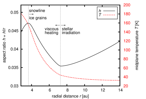
Figure 1: Radial profile of the aspect ratio $h(r)=H/r$ and temperature $T(r)$ in the disk used in our simulations. The right vertical dotted line marks the transition between the viscously heated and stellar irradiated regions, the latter exhibiting flaring of the disk. The left vertical dotted line corresponds to the water ice line which is also a local maximum of the Bell & Lin (1994) opacities. The figure is taken from Chrenko et al. (2017).

The protoplanetary disk model used in all our RHD simulations is exactly the same as in Chrenko et al. (2017), including the initial and boundary conditions (de Val-Borro et al., 2006). The parameters characterizing the initial gas disk are the surface density $\Sigma=750(r/(1\,\mathrm{au}))^{-0.5}\,\mathrm{g}\,\mathrm{cm}^{-2}$, kinematic viscosity $\nu=5\times 10^{14}\,\mathrm{cm}^{2}\,\mathrm{s}^{-1}$, adiabatic index $\gamma=1.4$, mean molecular weight $\mu=2.4\,\mathrm{g\,mol^{-1}}$, vertical opacity drop $c_{\kappa}=0.6$ and disk albedo $A=0.5$. The central star has the effective temperature $T_{\star}=4370\,\mathrm{K}$, stellar radius $R_{\star}=1.5\,R_{\sun}$ and mass $M_{\star}=1\,M_{\sun}$. The domain stretches from $r_{\mathrm{min}}=2.8\,\mathrm{au}$ to $r_{\mathrm{max}}=14\,\mathrm{au}$ in radius and spans the entire azimuth, having the grid resolution $1024\times 1536$ (rings $\times$ sectors).

The gas disk is numerically evolved to its thermal equilibrium and only after that, the coupled pebble disk is introduced. Pebbles are parametrized by the radial pebble mass flux $\dot{M}_{\mathrm{F}}=2\times 10^{-4}\,M_{\earth}\,\mathrm{yr}^{-1}$ (Lambrechts & Johansen, 2014), the Schmidt number $\mathrm{Sc}=1$, coagulation efficiency $\epsilon_{\mathrm{p}}=0.5$ (Lambrechts & Johansen, 2014), bulk density $\rho_{\mathrm{b}}=1\,\mathrm{g}\,\mathrm{cm}^{-3}$ and turbulent stirring efficiency $\alpha_{\mathrm{p}}=1\times 10^{-4}$ (e.g. Youdin & Lithwick, 2007). To infer the pebble sizes, we assume the drift-limited growth regime (Birnstiel et al., 2012; Lambrechts & Johansen, 2014) leading to pebble sizes of several $\mathrm{cm}$.

For reference, Figure 1 shows the radial profiles of the aspect ratio $h(r)=H/r$ and temperature $T(r)$ of the equilibrium gas disk. The $h(r)$ profile has a maximum near $4\,\mathrm{au}$ where the opacity peaks just before the sublimation of water ice (Bell & Lin, 1994). Therefore the heat produced by viscous heating is not easily radiated away from this opaque region and the disk puffs up.

Near $7\,\mathrm{au}$, the disk starts to flare because the vertical optical depth is small enough for the incoming radiation to penetrate deeper and heat the disk. The transition to the flared outer parts produces a zone of convergent Type I migration for planetary embryos (Bitsch et al., 2013; Pierens, 2015).

3.2 Nominal simulation

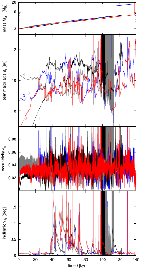
Figure 2: Temporal evolution of the embryo masses $M_{\mathrm{em}}$ (top), stellarcentric semimajor axes $a_{\mathrm{s}}$ (second row), eccentricities $e_{\mathrm{s}}$ (third row) and inclinations $I_{\mathrm{s}}$ (bottom) in the full RHD simulation with the gas disk, pebble disk, pebble accretion and accretion heating. Initially, there are four migrating embryos, numbered inside out. The inclination starts at $I_{0}=10^{-3}\,\mathrm{rad}$, which is also a value under which the inclination damping is switched off in the model. The strong variations of the stellarcentric Keplerian elements between $\simeq$$98\,\mathrm{kyr}$ and $\simeq$$114\,\mathrm{kyr}$ are a consequence of binary planet formation. A member of the binary swaps for one of the accompanying embryos three times as indicated by the change in colors of the oscillating curves (from a narrow strip of red to black and to gray). The existence of the binary ends abruptly by a merger (clearly related to the instantaneous mass increase in the $M_{\mathrm{em}}(t)$ plot).

Let us now discuss and analyze our nominal simulation in which binary planets were found to form. Initially, we set four embryos on circular orbits with stellarcentric semimajor axes ${a_{\mathrm{s}}}=5,6.7,8.4$ and $10.1\,\mathrm{au}$, inclinations ${I_{\mathrm{s}}=}I_{0}=10^{-3}\,\mathrm{rad}\simeq 0.057^{\circ}$ and randomized longitudes. The initial mass of each embryo is ${M_{\mathrm{em}}}=3\,{M}_{\earth}$ and their orbital separations are equal to $16$ mutual Hill radii

$$R_{\mathrm{mH},ij}=\frac{a_{\mathrm{s},i}+a_{\mathrm{s},j}}{2}\left(\frac{M_{\mathrm{em},i}+M_{\mathrm{em},j}}{3M_{\star}}\right)^{1/3}\,.$$ (10)

Embryos are numbered $1,2,3$ and $4$ from inside out.

Figure 2 shows the evolution of embryos over $140\,\mathrm{kyr}$ of the full RHD simulation with pebble accretion and respective heating. At first, the embryos undergo convergent migration towards their zero-torque radius. Without the heating torques, the embryos would concentrate near $7\,\mathrm{au}$ thanks to the contribution of the entropy-related corotation torque (Paardekooper & Mellema, 2008) which is positive between $\simeq$$4$ to $7\,\mathrm{au}$ in this particular disk model.

With the heating torques, however, the zero-torque radius is shifted further out because these torques are always positive (Benítez-Llambay et al., 2015). Moreover, the hot-trail effect quickly excites orbital eccentricities. Within $\simeq$$2\,\mathrm{kyr}$, the eccentricities reach up to ${e_{\mathrm{s}}}\simeq 0.02$ for the innermost embryo and ${e_{\mathrm{s}}}\simeq 0.04$ for the outermost embryo.

The inclinations first remain constant near the prescribed $I_{0}$ value, with only small temporal excitations not exceeding ${I_{\mathrm{s}}}\simeq 0.2^{\circ}$. Even these initially small inclinations are enough to modify the encounter geometries in a way that the system becomes gradually stirred in the vertical direction. Once the system becomes closely packed, at about $\simeq$$35\,\mathrm{kyr}$ into the simulation, the mutual close encounters pump the inclinations significantly, typically to ${I_{\mathrm{s}}}\simeq 1^{\circ}$ and even up to ${I_{\mathrm{s}}}\simeq 2^{\circ}$. Planets can pass above or below each other because their vertical excursions are comparable to (or larger than) their Hill spheres. For example, the maximal vertical excursion of a $5\,M_{\earth}$ embryo at $10\,\mathrm{au}$ is $z_{\max}\simeq 2R_{\mathrm{H}}$ when ${I_{\mathrm{s}}}=2^{\circ}$.

Due to excited eccentricities, the embryos never form a stable resonant chain, in accordance with Chrenko et al. (2017). Moreover, the excited inclinations help the embryos to avoid collisions and mergers for a long period of time. Consequently, close encounters of embryos are frequent in the system. Between $\simeq$$98\,\mathrm{kyr}$ and $\simeq$$114\,\mathrm{kyr}$, strong unphysical oscillations of the stellarcentric orbital elements appear in Figure 2 for some of the embryos, indicating formation of gravitationally bound binary planets.

3.3 Gravitationally bound pairs of embryos

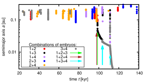
Figure 3: The record of all relative 2-body orbits satisfying the condition $a<R_{\mathrm{mH}}$ and $e<1$ in our nominal simulation. The filled circles mark the instantaneous semimajor axis and each pair of embryos is distinguished by color. The arrows are used to indicate when a gravitationally bound pair participates in a 3-body encounter.

To identify the events related to the binary formation in the simulation described above, we computed orbits of the relative motion among all possible pairs of embryos and selected those with $a<R_{\mathrm{mH}},e<1$. The results are shown in Figure 3. Throughout the simulation, we found $65$ time intervals during which at least two embryos are captured on a mutual elliptic orbit, changing their relative orbital energy from initially positive to negative (and back to positive when the capture terminates). Subsequently, we also scanned the sample of bound pairs and looked for cases when a third embryo has its distance from a pair $d<R_{\mathrm{mH}}$ to identify 3-body (pair-embryo) encounters. These are highlighted in Figure 3 by arrows.

Analyzing the lifetime of the bound pairs, we found that most of them dissolve before finishing one stellarcentric orbit. However, we found a single case when several binary configurations existed consecutively for a prolonged period of time between $\simeq$$98\,\mathrm{kyr}$ and $\simeq$$114\,\mathrm{kyr}$. This time interval is bordered by 3-body encounters which usually cause the binary separation to drop.

In summary, bound pairs can form in 2-body encounters but they quickly dissolve unless they undergo a 3-body encounter with one of the remaining embryos. The latter process is known as binary hardening (e.g. Hills, 1975, 1990; Goldreich et al., 2002; Astakhov et al., 2005) and it occurs when an external perturber removes energy from a binary system which then becomes more tightly bound. To distinguish among two types of events contributing to the formation of bound pairs, we call those formed in 2-body encounters transient binaries because of their typically short dynamical lifetime.

The transient binaries have been a subject of many different studies, for example, in the 3-body Hill problem (e.g. Simó & Stuchi, 2000; Astakhov et al., 2005). Their formation is possible because the orbital energy of two bodies in no longer conserved when additional perturbers (e.g. the central star) are present (e.g. Cordeiro et al., 1999; Araujo et al., 2008). Our system is of course more complicated because additional gravitational perturbations arise from the gas disk. We will demonstrate in Section 3.4 that the gas indeed facilitates formation of transients.

One last question we address here is whether or not the occurrence of bound pairs in Figure 3 is related to the vertically stirred orbits of embryos. To find an answer, we looked for bound pairs (with $a<R_{\mathrm{mH}},e<1$) in one of our previous simulations reported in Chrenko et al. (2017) (dubbed Case III), where the inclinations were damped in the standard way (Tanaka & Ward, 2004). We found only $6$ bound pairs (all transients) compared to $65$ cases in our nominal simulation presented here. Therefore, the excited inclinations importantly change the outcomes of embryo encounters in the gas disk and help to form transients.

3.4 Transient binary formation in a 2-body encounter

(a)	(b)	(c)
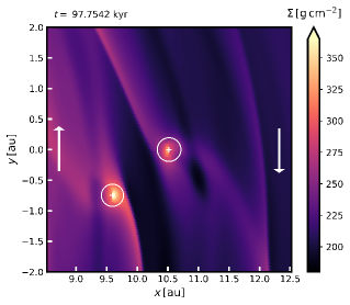
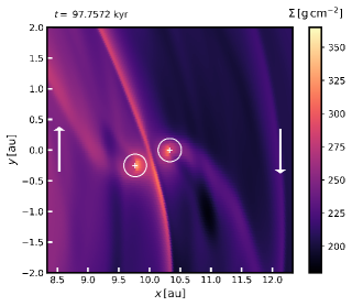
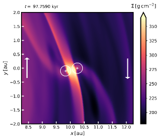
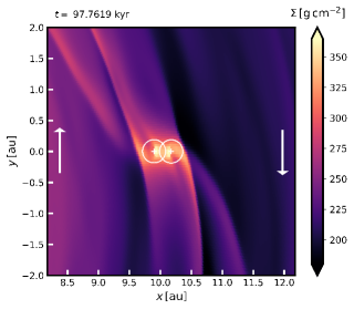
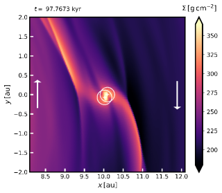
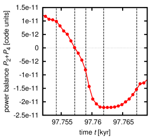
(d)	(e)	(f)

Figure 4: Formation of a transient binary during a 2-body encounter of embryos 2 and 4. The first five panels (a)–(e) show the evolution of the perturbed surface gas density $\Sigma$. Locations of the embryos are marked by white crosses, their Hill spheres are indicated by white circles and white arrows show the direction of the Keplerian shear in the reference frame corotating with the embryo 2 which is placed at the center of each plot. The individual panels are labeled with the simulation time $t$. The final panel (f) shows the evolution of the total power of the gravitational forces exerted by the disk onto embryos 2 and 4. The vertical dashed lines mark the simulation time corresponding to the snapshots of $\Sigma$ in panels (a)–(e). An animation of the formation of the transient binary is available in the online Journal and covers $t\simeq 97.73$–$97.8\,\mathrm{kyr}$ in simulation time.

Here we investigate formation of a transient pair of embryos $2$ and $4$ which precedes the binary hardening events in our nominal simulation. The pair forms in a 2-body interaction at $t\simeq 97.76\,\mathrm{kyr}$. To see whether the embryo-disk interactions assist in the process, we show in Figure 4 the evolution of the perturbed gas surface density $\Sigma$ during the encounter.

Before the encounter (panel (a)), the usual structures can be seen in the disk. The hot (underdense) trail of the outer embryo 2 can be seen as a dark oval spot in the bottom right quadrant (it moves down and gets larger in time). The hot trail of the inner embryo 4 is less prominent and looks as an underdense gap attached to the embryo from inside.

As the embryos approach in panel (b), the outer spiral arm of the inner embryo 4 and the inner spiral arm of the outer embryo 2 join and overlap. The overlap forms a strong density wave positioned between the embryos. The overdensity increases as part of the wave becomes trapped between the Hill spheres of both embryos in panel (c). From panel (c) to (d), the embryos cross this shared density wave.

In panel (d), the embryos are so close to each other that they effectively act on the disk as a single mass and the previously shared spiral arm splits into an inner and outer component with a small pitch angle. There are two more spirals with a larger pitch angle which are leftovers of the initial wakes launched by the embryos. In panel (e), all spirals blend into a single pair of arms. The embryos enter one another’s Hill sphere between panels (d) and (e) through the vicinity of the Lagrange points $\mathrm{L}_{1}$ for the outer and $\mathrm{L}_{2}$ for the inner embryo, respectively (Astakhov et al., 2005). The embryos are captured on a prograde binary orbit (in panel (e), the embryo 4 orbits the central embryo 2 counterclockwise).

The spiral arm crossing which appears during the encounter is known to produce strong damping effects onto the embryos (Papaloizou & Larwood, 2000). It is thus likely that the gas supports the gravitational capture by dissipating the orbital energy. To quantify this effect, we measured the total gravitational force $\vec{F}_{\mathrm{g},i}$ exerted by the disk onto each embryo and we calculated the mechanical power

$$P_{i}=\int\limits_{\mathrm{disk}}\vec{v}_{i}\cdot\vec{F}_{\mathrm{g},i}\mathrm{d}S\,,$$ (11)

where $\vec{v}_{i}$ is the velocity vector of the embryo and the integral goes over the entire disk. $P_{i}$ directly determines the rate of change of the orbital energy $\dot{E}_{i}$ of each embryo (e.g. Cresswell et al., 2007).

Panel (f) of Figure 4 shows the total balance of the energy subtraction (or addition) for the embryos $2$ and $4$, $P=P_{2}+P_{4}$. The energy is transfered to the disk when $P<0$ and vice versa. It is obvious that throughout the closest approach (panels (b)–(e)), the orbital energy of the embryos dissipates and thus the influence of the gas disk on formation of transients is confirmed.

3.5 Binary planet hardening in 3-body encounters

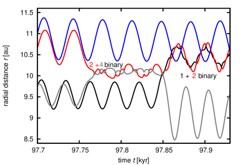
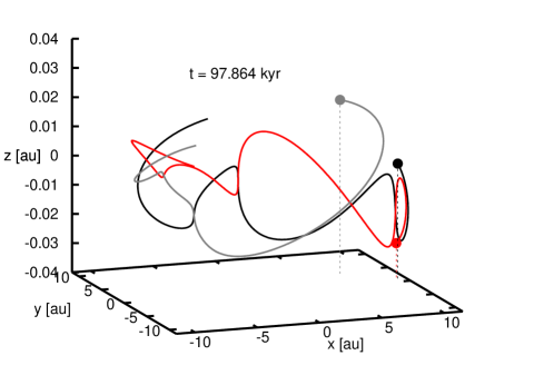
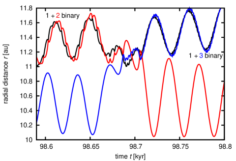
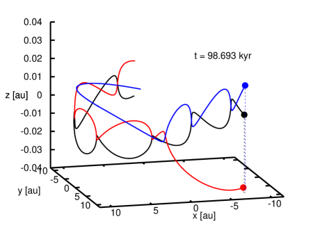
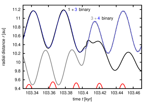
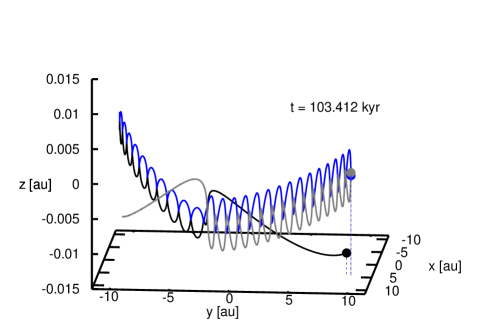
Figure 5: Details of important 3-body encounters occurring in the nominal simulation, leading to reconfiguration and hardening of the binary planet. Each row shows a different encounter (and the first row also shows the transient binary of embryos 2+4 preceding the 3-body encounters). We plot the temporal evolution of the radial distance $r$ (left column) and also the orbital evolution in 3D Cartesian space (right column) in a short time interval around the respective encounters. The numbering and coloring of the bodies is the same as in Figure 2. Filled circles in the right column mark the positions of embryos at the simulation time $t$ given by the labels. An animated version of the top row of Figure 5 is available in the online Journal. The animation spans $t\simeq 97.7$–$97.92\,\mathrm{kyr}$ in simulation time, displaying the same tracks as in the static figure.

The transient pair of embryos $2$ and $4$ does not dissolve, instead it is further stabilized in 3-body encounters with the remaining embryos. Figure 5 shows these encounters in detail. First, the transient pair encounters embryo $1$ at $t\simeq 97.85\,\mathrm{kyr}$. During this encounter, one component of the binary (embryo $4$) becomes unbound and is deflected away but the incoming embryo $1$ takes its place in an exchange reaction so the binary does not cease to exist.

Similar situation repeats at about $\simeq$$98.69\,\mathrm{kyr}$ when the configuration $1+2$ changes to $1+3$ and at $\simeq$$103.4\,\mathrm{kyr}$ when the configuration $1+3$ changes to $3+4$. Figure 5 also reveals the binary becomes hardened with each encounter since the overlap between the $r(t)$ curves for the binary components becomes tighter.

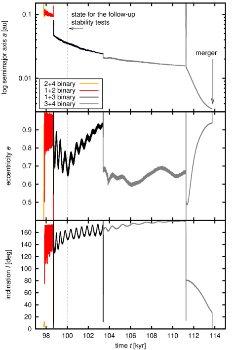
Figure 6: The temporal evolution of the orbital elements of the binary planet, namely the semimajor axis $a$ (top), eccentricity $e$ (middle) and inclination $I$ (bottom). The color of the curves changes if different embryos become locked in the binary configuration during a 3-body encounter (see Figure 5 for reference). The encounters can be recognized as sudden spikes and they typically lead to a sudden decrease of $a$ and $e$. In the course of time, the binary becomes bound more tightly. The existence of the binary ends with a merger, marked by an arrow.

Even clearer indication of the binary hardening is provided by Figure 6 where we plot the temporal evolution of the orbital elements of the binary planet. The color of the curves changes each time there is a change in the composition of the binary. One can further notice the exchange interactions produce sudden decreases of $a$ and also of $e$. Between the exchange interactions, $a$ smoothly decreases whereas $e$ generally increases in an oscillatory manner. We will describe these variations later.

Considering the binary planet inclination, the transient binary $2+4$ forms with a prograde orbit and a relatively low inclination. During the first 3-body encounter, the binary is reconfigured to retrograde orbit with the inclination oscillating between $100^{\circ}$ and $170^{\circ}$. The inclination then slowly evolves towards $180^{\circ}$ regardless of the swap encounters which only diminish the oscillation amplitude.

The binary planet does not survive to the end of our simulation. At $\simeq$$111.26\,\mathrm{kyr}$, it undergoes a 3-body exchange interaction with the embryo $1$ during which their Hill spheres overlap for a prolonged period of time (see the spike in Figure 3 at $\simeq$$111.26\,\mathrm{kyr}$). Consequently, the binary inclination is flipped from the retrograde configuration to $I=80^{\circ}$. In this configuration, the binary undergoes fast decrease of $a$, accompanied by an equally fast increase of $e$. Consequently, the binary planet ends its life in a merger into a single body.

3.6 Binary planet evolution without perturbing embryos

The lifetime of the hardened binary in our nominal simulation is long enough ($\sim$$10^{4}\,\mathrm{yr}$) to be interesting. There are two basic questions that we shall now address. First, what is the evolution of such a binary if the surrounding embryos and their perturbations are ignored? And second, what causes the changes of the binary orbital elements between the 3-body encounters in Figure 6?

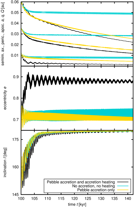
Figure 7: Stability test starting from the binary planet configuration corresponding to $t=100\,\mathrm{kyr}$ in Figure 6. In this test, the surrounding planetary embryos are removed. Therefore we study evolution of an isolated binary driven only by its interactions with the disk and not by close encounters. Three cases are shown: One with the complete RHD and two-fluid part of the model (black curve), one with pebble accretion but without accretion heating (gold curve), and one without both pebble accretion and heating (turquoise curve). Pebble accretion (i.e. mass growth) of the embryos generally causes the semimajor axis decrease. Accretion heating, on the other hand, is capable of pumping the eccentricity above the initial value.

To answer these questions, we discard the non-binary embryos and restart the simulation from the configuration of the binary planet, gas and pebbles corresponding to $t=100\,\mathrm{kyr}$. Three models are numerically evolved for $45\,\mathrm{kyr}$. The first one has the same setup as the initial simulation (apart from the ignored non-binary embryos). In the second one, the accretion heating is disabled but the mass of the binary components can still grow by pebble accretion. In the third one, we again switch off accretion heating and discard the pebble disk; the binary mass therefore remains constant.

The orbital evolution of the binary in these three cases is shown in Figure 7. The inclination evolution is more or less the same, regardless of the model, and converges toward a fully retrograde configuration. The semimajor axis decreases as a consequence of pebble accretion which transports the linear momentum and mass onto the binary components, thus changing their orbital angular momentum. It is worth noting that if the pebble accretion and accretion heating are ignored, the isolated binary planet evolving in the radiative disk exhibits only minor orbital changes (once it adjusts to the removal of the surrounding embryos at the beginning of the restart).

The eccentricity substantially changes only in the model with accretion heating, otherwise it oscillates around its initial value or exhibits a slow secular variation. In other words, the hot-trail effect is important not only for exciting the eccentricities of individual embryos before the encounter phase, but it is also responsible for pumping the eccentricity of the binary up to an asymptotic value $e\simeq 0.75$.

These findings justify our incorporation of pebble accretion and accretion heating into the model because both phenomena affect the rate of change of the binary orbital elements. Pebble accretion diminishes the semimajor axis and accretion heating excites the eccentricity.

3.7 Binary planet evolution in the disk-free phase

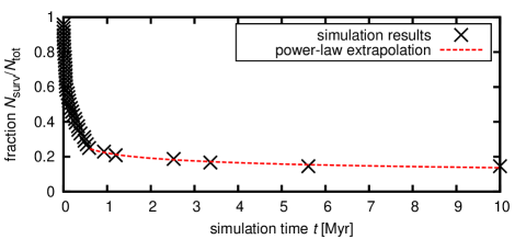
Figure 8: The fraction of N-body integrations in which the binary planets survives until simulation time $t$. The crosses mark the results of our integrations, the dashed curve is a power-law fit which is used as an extrapolation for $t>10\,\mathrm{Myr}$.

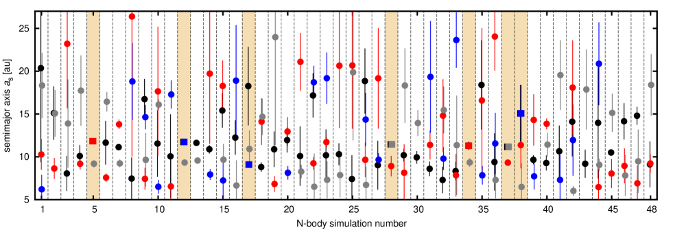
Figure 9: Orbital distribution of the planetary systems $10\,\mathrm{Myr}$ after the disk removal. The horizontal axis shows the reference number of N-body simulations, individual cases are separated by the vertical dashed lines. The vertical axis shows the stellarcentric semimajor axis of planets displayed with symbols (the coloring is the same as in the previous figures). Single planets are marked by filled circles, binary planets are distinguished by filled squares (squares correspond to $a_{\mathrm{s}}$ of the binary barycenter). The systems which preserved the binary are also highlighted using the yellow background. The vertical bars of each symbol indicate the span of orbits from pericenter to apocenter (large bars correspond to eccentric orbits and vice versa).

When protoplanetary disks undergo dispersal due to photoevaporation, the emerging planetary systems may become unstable (e.g. Lega et al., 2013). Here we test whether the hardened binary planet could survive the gas removal phase and the subsequent orbital instabilities. Since the binary undergoes 3-body encounters during the disk phase, they can be expected also after the disk removal.

To investigate the evolution after the photoevaporation, we remove the fluid part of the model (i.e. gas and pebbles) instantly and continue with a pure N-body simulation. The orbits are integrated for additional $10\,\mathrm{Myr}$. To account for the chaotic nature of an N-body system with close encounters, we extract $48$ orbital configurations of the embryos from between $\simeq$$99.7\,\mathrm{kyr}$ and $\simeq$$102.4\,\mathrm{kyr}$ of the nominal simulation and use them as the initial conditions for $48$ independent integrations.

Our aim is to quantify the binary planet survival rate. Figure 8 shows the evolution of the fraction $N_{\mathrm{surv}}/N_{\mathrm{tot}}$, where $N_{\mathrm{surv}}$ is the number of N-body systems still containing a binary planet at simulation time $t$ and $N_{\mathrm{tot}}$ is the total number of systems (48). The dependence exhibits a steep decrease — the binary dissolves before $0.1\,\mathrm{Myr}$ of evolution in $\simeq$$45\,\%$ of cases and before $1\,\mathrm{Myr}$ in $\simeq$$76\,\%$ of cases. However, the trend for $t\geq 1\,\mathrm{Myr}$ becomes rather flat. The binary planet survives the whole integration timespan in $15\,\%$ of our runs.

We estimate the fraction of planetary systems $f_{\mathrm{surv}}$ in which the binary can survive the orbital instabilities. An estimate for young systems can be readily done by taking the final fraction of our integrations conserving the binary, yielding $f_{\mathrm{surv},10\,\mathrm{Myr}}\simeq 15\%$. To make an estimate for older systems, we performed a power-law extrapolation of the flat tail of the distribution in Figure 8. The resulting extrapolation $0.22(t/(1\,\mathrm{Myr}))^{-0.21}$ yields $f_{\mathrm{surv},4.5\,\mathrm{Gyr}}\simeq 4\%$ for $t=4.5\,\mathrm{Gyr}$ (i.e. comparable to the Solar System age).

Let us briefly discuss the orbital architecture of the individual systems at the end of our integrations (Figure 9). Focusing on the systems which retained the binary, they can be divided into two classes. The more common first class comprises five systems (simulation number $5,12,28,34,37$) in which one of the binary components undergoes an early collision (at about $\simeq 0.1\,\mathrm{Myr}$) with one of the remaining embryos while maintaining the binary configuration. The collision reduces the multiplicity of the system and changes the mass ratio of the binary components from $1/1$ to $2/1$. The stability of such systems is obvious from Figure 9 because eccentricities are only marginally excited and the planets do not undergo orbital crossings.

The less frequent second class of orbital architectures (simulation number $17$ and $38$) includes systems in which no collision occurred yet the binary managed to survive close encounters. Orbits of the single embryos in these simulations are moderately eccentric and have orbital crossings with the binary. It is very likely that these systems would reconfigure and the binary would dissolve when integrating for $t>10\,\mathrm{Myr}$. We however believe that these two cases are accounted for by the power-law extrapolation when estimating $f_{\mathrm{surv}}$ for old systems.

3.8 Formation efficiency

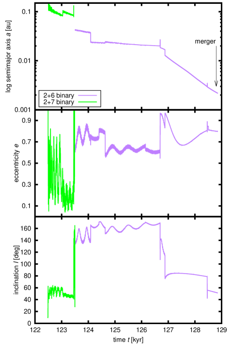
Figure 10: As Figure 6, but for the binary configurations found in our additional simulation IV with 8 embryos (initial $M_{\mathrm{em}}=1.7\,\mathrm{M_{\earth}}$). The binary shown here undergoes similar evolution to that in Figure 6.

So far the analysis was based on our nominal simulation. Although a broader study of the parametric space is difficult using RHD simulations, it is important to quantify how common it is for transients to become hardened and stabilized in 3-body encounters. Also, it is desirable to test if the result is sensitive to the choice of initial separations, embryo masses and embryo multiplicity.

We perform four additional full RHD simulations in which we vary the initial conditions for embryos (the disk remains the same as in Section 3.1). Embryos start with different random longitudes and inclinations are $I_{\mathrm{s}}=I_{0}$. Two simulations (denoted I and II) are run with 4 embryos, each having $M_{\mathrm{em}}=3\,\mathrm{M_{\earth}}$ again, but the innermost embryo is initially placed at $a_{\mathrm{s}}=6\,\mathrm{au}$ and the remaining ones are spaced by $10$ mutual Hill radii. Two simulations (denoted III and IV) include 8 embryos with $M_{\mathrm{em}}=1.7\,\mathrm{M_{\earth}}$, the inner one being placed at $a_{\mathrm{s}}=5\,\mathrm{au}$ and the others having initial separations of $8$ mutual Hill radii.

The simulations I and II cover $120\,\mathrm{kyr}$ of evolution. A common feature of these runs is a merger occurring relatively early (at $\simeq$$40\,\mathrm{kyr}$ and $\simeq$$51\,\mathrm{kyr}$ in simulations I and II, respectively), followed by a second merger (at $\simeq$$81\,\mathrm{kyr}$ and $\simeq$$94\,\mathrm{kyr}$ in simulations I and II, respectively). The simulation III covers $180\,\mathrm{kyr}$ of evolution. There is a late violent sequence at $\simeq 150\,\mathrm{kyr}$ during which 2 mergers occur and 3 embryos are scattered out of the simulated part of the disk.

In simulations I–III, only transient binaries are formed. However, we detect one case of a hardened binary in the simulation IV which covers $120\,\mathrm{kyr}$ of evolution. The simulation also contains 190 transients compared to 65 cases found in our nominal simulation which implies that the increased multiplicity of the system (8 instead of 4 embryos) logically increases the frequency of embryo encounters.

Figure 10 shows the evolution of orbital elements of the binary configurations participating in binary hardening. First, a transient consisting of embryos $2$ and $7$ forms at about $122.5\,\mathrm{kyr}$. After $\simeq 1\,\mathrm{kyr}$, it undergoes a 3-body encounter during which the configuration changes to embryos $2$ and $6$ and the binary semimajor axis decreases. Then the binary evolves for about $5\,\mathrm{kyr}$ due to pebble accretion and additional 3-body encounters. The secular rate of change of $a$ is clearly related to the value of $I$, suggesting that the deposition of pebbles onto a prograde binary causes the separation to decrease faster compared to a retrograde case. As in the nominal simulation, the binary separation shrinks until the binary merges.

Although the statistics of our 5 (1 nominal and 4 additional) RHD simulations is still poor, we can nevertheless conclude that a binary planet with considerable lifetime can form at least in some cases. We can also make a crude estimate of the formation efficiency $f_{\mathrm{form}}$ which we define as a fraction of simulations in which a binary planet was formed and then hardened, obtaining $f_{\mathrm{form}}\simeq 0.4$.

For simulations which formed such binaries, we also define the total time $\tau_{\mathrm{bp}}$ for which the binary planet existed in the system (regardless of which embryos were bound). The binary in our nominal simulation existed for $\simeq$$16\,\mathrm{kyr}$ and the binary in the simulation IV existed for $\simeq$$6\,\mathrm{kyr}$ in total. Taking the arithmetic mean of these two values we obtain $\tau_{\mathrm{bp}}\simeq 11\,\mathrm{kyr}$.

4 Discussing binary planets

4.1 Model complexity and limitations

The choice of the RHD model was not a priori motivated by studying formation of binary planets. The initial motivation was to check how the evolution described in Chrenko et al. (2017) changes if the orbits of embryos become inclined due to the vertical hot-trail effect (only the horizontal hot-trail was modelled in Chrenko et al., 2017). We found binary planet formation as an unexpected yet natural outcome of the model.

It is possible that a less complex model could be applied to scan the parametric space, e.g. by N-body integrations. But although there are many state-of-the-art N-body models of migration in multiplanet systems with disks (e.g. Cossou et al., 2013, 2014; Izidoro et al., 2017), none of them (to our knowledge) identified formation of binary planets. This suggests that there might be issues preventing binary planet formation in such models.

We demonstrated in Section 3.4 that hydrodynamic effects are important during formation of transient binaries by 2-body encounters. The pair of approaching embryos creates perturbations in the disk which differ from perturbations arising from isolated embryos. The prescriptions for the disk torques which are currently used in N-body models (Paardekooper et al., 2010, 2011; Cresswell & Nelson, 2008; Fendyke & Nelson, 2014) cannot account for such effects because they were derived from models containing a single embryo, not an interacting pair. Moreover, such prescriptions do not account for the thermal torque and hot-trail effect.

We point out that our RHD model has some limitations as well. First, although the grid resolution leads to numerical convergence of the migration rate for low-mass planets (see e.g. Lega et al., 2014; Brož et al., 2018, for resolution discussions), it is not tuned to resolve binary configurations with the smallest orbital separations well enough. However, looking at the turquoise curve in Figure 7 (i.e. the case without additional perturbers), the marginal change of orbital elements indicates very low level of numerical dissipation, safely negligible over a typical binary lifetime during the disk phase. Second, the vertical hot-trail cannot be implemented in our 2D model in a self-consistent way. 3D simulations would be required to assess the importance of the vertical dimension which we neglect here. Finally, the magnitude of the thermal torques depends on the thermal diffusivity and therefore on the opacity (Masset, 2017). However, we used a single opacity prescription and it remains unclear if the described effects work the same way e.g. in a low-density disk undergoing photoevaporation.

4.2 Formation mechanism

We found that 2-body encounters of planetary embryos in the gas disk can establish transient binaries. A binary planet with a considerable lifetime can form from a transient by a 3-body encounter which provides the necessary energy dissipation to make the pair more tightly bound. Here we discuss whether there are other mechanisms suitable for formation of binary planets.

Additional possibility exists during the reaccumulation phase after a large impact of two embryos approaching on initially unbound trajectories, as discussed by Ryan et al. (2014). But this situation is highly unlikely. Head-on collisions usually disrupt the protoplanets in a way that the reaccumulation forms a large primary and a low-mass disk, from which a satellite can be assembled but not a binary companion. Only a special grazing geometry with a large impact parameter can be successful (Ryan et al., 2014) and it can only produce binaries with separations of a few planetary radii due to the angular momentum deficit of such an encounter.

Finally, planets can be captured in a binary configuration by means of the tidal dissipation. Ochiai et al. (2014) studied the evolution of three hot Jupiters around a host star and discovered that binary gas giants can form in $\sim$$10\%$ of systems which undergo orbital crossings.

4.3 Mass of the binary

In our hydrodynamic simulations, the components of binaries have comparable masses of several $M_{\earth}$ before they merge. But as we found in the follow-up gas-free N-body simulations, the system often stabilizes by a collision of one of the embryos onto the binary. If the binary survives the collision, the mass ratio of the components increases to $2/1$. Therefore it seems that if born from a population of equal mass embryos (as obtained in the oligarchic growth scenarios), binary planets would preferentially exist with the component mass ratios $1/1$ or $2/1$. This aspect of our model is related to the choice of the initial embryo masses and is of course too simplified to capture the outcome of models where accretion creates a range of embryo masses.

Although simulations with gas accretion onto the planets are beyond the scope of our paper, we believe that runaway accretion of gas onto the binary would disrupt it. We thus expect the binary planets formed in 3-body encounters cannot exceed the masses of giant planet cores. This could be ensured by the mechanism of pebble isolation (Lambrechts et al., 2014; Bitsch et al., 2018) or simply because binaries could form late, just before the gas disk dispersal. However, it is possible that binary giant planets form later by the mechanism of tidal capture (Ochiai et al., 2014).

4.4 Tidal evolution

Orbital evolution due to tidal dissipation is without any doubts an important factor for the stability of binary planets. However, it is difficult to assess the tidal effects at this stage because there are many unknown parameters. Large uncertainty lies in the $k_{2}/Q$ parameter, where $k_{2}$ is the degree 2 Love number and $Q$ is the tidal quality factor (e.g. Harris & Ward, 1982). These parameters reflect the interior structure and thus they depend on the planetary composition (water-rich vs silicate-rich) and state (cold vs magma worlds), the latter of which changes on an uncertain timescale. Moreover, our model treats the planets as point-mass objects, therefore we have no information about their rotation which is important to determine the level of spin-orbital synchronicity. Additionally, similar masses of the binary components and their (possibly) retrograde and highly eccentric orbit make the analysis of tides even more complicated. For all these reasons, the model of tidal evolution of a binary planet should be sufficiently complex and should account for the internal structure and rheology (e.g. Boué et al., 2016; Walterová & Běhounková, 2017).

4.5 Occurrence rate and observability

We define the binary planet occurrence rate $f_{\mathrm{bp}}$ as the fraction of planetary systems which are expected to contain at least one binary planet hardened by 3-body encounters. An order-of-magnitude estimate can be obtained by dividing the time scale $\tau_{\mathrm{bp}}\simeq 10^{4}\,\mathrm{yr}$ for which these binary planets are typically present in our simulations (Section 3.8) by the lifetime of protoplanetary disks $\tau_{\mathrm{disk}}\simeq 10^{7}\,\mathrm{yr}$ (e.g. Fedele et al., 2010), correcting for the formation efficiency $f_{\mathrm{form}}\simeq 0.4$ (Section 3.8) and for the fraction of the emerging planetary systems $f_{\mathrm{stab}}$ in which the binary planet can survive after the gas disk dispersal (Section 3.7). This leads to

$$f_{\mathrm{bp}}=f_{\mathrm{form}}\frac{\tau_{\mathrm{bp}}}{\tau_{\mathrm{disk}}}f_{\mathrm{stab}}\,.$$ (12)

We quantify two characteristic values for young planetary systems (using $f_{\mathrm{stab},10\,\mathrm{Myr}}\simeq 0.15$) and for old planetary systems (using $f_{\mathrm{stab},4.5\,\mathrm{Gyr}}\simeq 0.04$), leading to $f_{\mathrm{bp},10\,\mathrm{Myr}}\simeq 6\times 10^{-5}$ and $f_{\mathrm{bp},4.5\,\mathrm{Gyr}}\simeq 2\times 10^{-5}$. In other words, one out of $\simeq$$2$–$5\times 10^{4}$ planetary systems should contain a binary planet formed by 2- and 3-body encounters.

We emphasize that the estimate is highly uncertain because it is inferred from a small number of tests. Moreover, our simulations cover only a small region of the protoplanetary disk, the evolution time scale is still short compared to the disk’s lifetime, and the number of embryos is relatively low. Last but not least, our estimate only assumes that binaries form by the processes identified in this work.

As pointed out in Section 1, the estimated occurrence rate should motivate a systematic search for binary planets in the observational data. For example, binary planets should be detectable by the Hunt for Exomoons with Kepler (HEK) project (Kipping et al., 2012). The sensitivity of this survey is $\simeq$$40\%$ for binaries with Pluto-Charon mass ratios (Kipping et al., 2015).

4.6 Role in planetary systems

Possible existence of binary planets opens new avenues in planetary sciences. A study of long-term orbital dynamics and stability of binaries in various systems is needed (e.g. Donnison, 2010), including an assessment of their tidal evolution. Binary planets are challenging for hydrodynamic modeling as well. Local high-resolution simulations of interactions with the disk, pebble accretion, pebble isolation (e.g. Bitsch et al., 2018) and gas accretion (e.g. Lambrechts & Lega, 2017) should be performed for binary planets (preferentially in 3D) to understand the impact of these processes in detail.

In this paper, we reported various fates of binary planets (considering the set of gas-free N-body simulations). Frequently, one of the binary components underwent a collision with an equally large impactor, or the binary merged. The merger of the binary planet is a process that should be investigated (e.g. by the smoothed-particle hydrodynamics (SPH) method, Jutzi, 2015).

A merger can occur in a situation when the binary orbit is inclined with respect to the global orbital plane and the resulting body would then retain the initial angular momentum of the binary, forming a planet (or a giant-planet core) with an angular tilt of the rotational axis. It might be worth investigating a relation of such an event to the origin of Uranus.

Moreover, the collision of the binary components would statistically occur on high impact angles. It is interesting that such impact angles and similar masses of the target and the impactor (although on unbound trajectories) were also used for successful explanation of the impact origin of the Earth-Moon system (Canup, 2012).

5 Conclusions

By means of 2D radiation hydrodynamic simulations with 3D planetary orbits, we described formation of binary planets in a system of migrating super-Earths. A key ingredient of the model is the vertical hot-trail effect (Eklund & Masset, 2017) which was incorporated by reducing the efficiency of the inclination damping prescription (Tanaka & Ward, 2004). We also accounted for the pebble disk, pebble accretion and accretion heating, which naturally produces the horizontal hot-trail effect, providing eccentricity excitation (Chrenko et al., 2017).

When convergent migration drives the planetary embryos together, the geometry of their encounters allows for vertical perturbations owing to the non-zero inclinations. The orbits become vertically stirred and dynamically hot, reaching inclinations up to $\simeq$$2^{\circ}$.

Numerous transient binary planets form during the simulations by gas-assisted 2-body encounters but such transients quickly dissolve. Binary planets with longer lifetimes $\sim$$10^{4}\,\mathrm{yr}$ form when a transient undergoes a 3-body encounter with a third embryo. During this process of binary hardening, energy is removed from the binary orbit and the separation of components decreases. Also, 3-body encounters often reconfigure the binary when one of the components swaps places with the encountered embryo. The existence of hardened binaries in our simulations typically ends with a merger of its components which forms a giant planet core.

The role of the gas disk for binary planet formation is twofold. In 2-body encounters, the disk can dissipate orbital energy of the embryos thus aiding the gravitational capture. The dissipation is provided when the embryos cross a shared spiral arm. Regarding 3-body encounters, the disk torques hold the embryos closely packed and the hot-trail effect maintains the eccentricities and inclinations excited, increasing the probability that a transient will encounter another embryo before it dissolves.

We conducted numerical experiments to test the stability and evolution of binary planets in cases when pebble accretion is halted, or accretion heating is inefficient, or the disk dissipates. We found that pebble accretion causes a secular decrease of $a$ of the binary whereas $e$ increases due to the hot-trail effect.

For the binary to survive after the disk dispersal, it is required that the surrounding embryos are removed or reconfigured dynamically. Quite often, a stable configuration is achieved when one of the components of the surviving binary undergoes a merger with another embryo, increasing the binary mass ratio from approximately $1/1$ to $2/1$.

We roughly estimated the expected fraction of planetary systems with binary planets to be $f_{\mathrm{bp}}\simeq 2$–$6\times 10^{-5}$, where the upper limit holds for young planetary systems and the lower limit holds for $4.5\,\mathrm{Gyr}$ old systems. In other words, a binary planet should be present in one planetary system out of $\simeq$$2$–$5\times 10^{4}$.

One can think of many new applications which the possible existence of binary planets brings. First, although binary planets are yet-to-be discovered, our occurrence rate estimate is encouraging for future observations. Second, the hydrodynamic interactions of binary planets with the disk may be different compared to a single planet and are worth investigating, preferably in 3D. Third, collisional models for planetary bodies which usually focus on unbound trajectories should also investigate colliding binaries to assess the possible outcomes.

References

- Araujo et al. (2008) Araujo, R. A. N., Winter, O. C., Prado, A. F. B. A., & Vieira Martins, R. 2008, MNRAS, 391, 675, doi: 10.1111/j.1365-2966.2008.13833.x
- Astakhov et al. (2005) Astakhov, S. A., Lee, E. A., & Farrelly, D. 2005, MNRAS, 360, 401, doi: 10.1111/j.1365-2966.2005.09072.x
- Baillié & Charnoz (2014) Baillié, K., & Charnoz, S. 2014, ApJ, 786, 35, doi: 10.1088/0004-637X/786/1/35
- Baruteau & Masset (2008) Baruteau, C., & Masset, F. 2008, ApJ, 672, 1054, doi: 10.1086/523667
- Bell & Lin (1994) Bell, K. R., & Lin, D. N. C. 1994, ApJ, 427, 987, doi: 10.1086/174206
- Ben-Jaffel & Ballester (2014) Ben-Jaffel, L., & Ballester, G. E. 2014, ApJ, 785, L30, doi: 10.1088/2041-8205/785/2/L30
- Benítez-Llambay et al. (2015) Benítez-Llambay, P., Masset, F., Koenigsberger, G., & Szulágyi, J. 2015, Nature, 520, 63, doi: 10.1038/nature14277
- Benítez-Llambay & Pessah (2018) Benítez-Llambay, P., & Pessah, M. E. 2018, ApJ, 855, L28, doi: 10.3847/2041-8213/aab2ae
- Bennett et al. (2014) Bennett, D. P., Batista, V., Bond, I. A., et al. 2014, ApJ, 785, 155, doi: 10.1088/0004-637X/785/2/155
- Birnstiel et al. (2012) Birnstiel, T., Klahr, H., & Ercolano, B. 2012, A&A, 539, A148, doi: 10.1051/0004-6361/201118136
- Bitsch et al. (2013) Bitsch, B., Crida, A., Morbidelli, A., Kley, W., & Dobbs-Dixon, I. 2013, A&A, 549, A124, doi: 10.1051/0004-6361/201220159
- Bitsch et al. (2018) Bitsch, B., Morbidelli, A., Johansen, A., et al. 2018, A&A, 612, A30, doi: 10.1051/0004-6361/201731931
- Boué et al. (2016) Boué, G., Correia, A. C. M., & Laskar, J. 2016, Celestial Mechanics and Dynamical Astronomy, 126, 31, doi: 10.1007/s10569-016-9708-x
- Brož et al. (2018) Brož, M., Chrenko, O., Nesvorný, D., & Lambrechts, M. 2018, ArXiv e-prints. https://arxiv.org/abs/1810.03385
- Brown et al. (2006) Brown, M. E., van Dam, M. A., Bouchez, A. H., et al. 2006, ApJ, 639, L43, doi: 10.1086/501524
- Brozović et al. (2015) Brozović, M., Showalter, M. R., Jacobson, R. A., & Buie, M. W. 2015, Icarus, 246, 317, doi: 10.1016/j.icarus.2014.03.015
- Canup (2011) Canup, R. M. 2011, AJ, 141, 35, doi: 10.1088/0004-6256/141/2/35
- Canup (2012) —. 2012, Science, 338, 1052, doi: 10.1126/science.1226073
- Chiang & Goldreich (1997) Chiang, E. I., & Goldreich, P. 1997, ApJ, 490, 368
- Chrenko et al. (2017) Chrenko, O., Brož, M., & Lambrechts, M. 2017, A&A, 606, A114, doi: 10.1051/0004-6361/201731033
- Christy & Harrington (1978) Christy, J. W., & Harrington, R. S. 1978, AJ, 83, 1005, doi: 10.1086/112284
- Cordeiro et al. (1999) Cordeiro, R. R., Martins, R. V., & Leonel, E. D. 1999, AJ, 117, 1634, doi: 10.1086/300764
- Cossou et al. (2014) Cossou, C., Raymond, S. N., Hersant, F., & Pierens, A. 2014, A&A, 569, A56, doi: 10.1051/0004-6361/201424157
- Cossou et al. (2013) Cossou, C., Raymond, S. N., & Pierens, A. 2013, A&A, 553, L2, doi: 10.1051/0004-6361/201220853
- Cresswell et al. (2007) Cresswell, P., Dirksen, G., Kley, W., & Nelson, R. P. 2007, A&A, 473, 329, doi: 10.1051/0004-6361:20077666
- Cresswell & Nelson (2008) Cresswell, P., & Nelson, R. P. 2008, A&A, 482, 677, doi: 10.1051/0004-6361:20079178
- Crida et al. (2008) Crida, A., Sándor, Z., & Kley, W. 2008, A&A, 483, 325, doi: 10.1051/0004-6361:20079291
- D’Angelo et al. (2003) D’Angelo, G., Henning, T., & Kley, W. 2003, ApJ, 599, 548, doi: 10.1086/379224
- de Val-Borro et al. (2006) de Val-Borro, M., Edgar, R. G., Artymowicz, P., et al. 2006, MNRAS, 370, 529, doi: 10.1111/j.1365-2966.2006.10488.x
- Donnison (2010) Donnison, J. R. 2010, MNRAS, 406, 1918, doi: 10.1111/j.1365-2966.2010.16796.x
- Eklund & Masset (2017) Eklund, H., & Masset, F. S. 2017, MNRAS, 469, 206, doi: 10.1093/mnras/stx856
- Erikson et al. (2012) Erikson, A., Santerne, A., Renner, S., et al. 2012, A&A, 539, A14, doi: 10.1051/0004-6361/201116934
- Fedele et al. (2010) Fedele, D., van den Ancker, M. E., Henning, T., Jayawardhana, R., & Oliveira, J. M. 2010, A&A, 510, A72, doi: 10.1051/0004-6361/200912810
- Fendyke & Nelson (2014) Fendyke, S. M., & Nelson, R. P. 2014, MNRAS, 437, 96, doi: 10.1093/mnras/stt1867
- Fraser et al. (2017) Fraser, W. C., Bannister, M. T., Pike, R. E., et al. 2017, Nature Astronomy, 1, 0088, doi: 10.1038/s41550-017-0088
- Giuppone et al. (2012) Giuppone, C. A., Benítez-Llambay, P., & Beaugé, C. 2012, MNRAS, 421, 356, doi: 10.1111/j.1365-2966.2011.20310.x
- Goldreich et al. (2002) Goldreich, P., Lithwick, Y., & Sari, R. 2002, Nature, 420, 643, doi: 10.1038/nature01227
- Han (2008) Han, C. 2008, ApJ, 684, 684, doi: 10.1086/590331
- Harris & Ward (1982) Harris, A. W., & Ward, W. R. 1982, Annual Review of Earth and Planetary Sciences, 10, 61, doi: 10.1146/annurev.ea.10.050182.000425
- Heller (2014) Heller, R. 2014, ApJ, 787, 14, doi: 10.1088/0004-637X/787/1/14
- Heller (2018) —. 2018, A&A, 610, A39, doi: 10.1051/0004-6361/201731760
- Hills (1975) Hills, J. G. 1975, AJ, 80, 809, doi: 10.1086/111815
- Hills (1990) —. 1990, AJ, 99, 979, doi: 10.1086/115388
- Hippke (2015) Hippke, M. 2015, ApJ, 806, 51, doi: 10.1088/0004-637X/806/1/51
- Hubeny (1990) Hubeny, I. 1990, ApJ, 351, 632, doi: 10.1086/168501
- Izidoro et al. (2017) Izidoro, A., Ogihara, M., Raymond, S. N., et al. 2017, MNRAS, 470, 1750, doi: 10.1093/mnras/stx1232
- Jutzi (2015) Jutzi, M. 2015, Planet. Space Sci., 107, 3, doi: 10.1016/j.pss.2014.09.012
- Kipping (2009) Kipping, D. M. 2009, MNRAS, 392, 181, doi: 10.1111/j.1365-2966.2008.13999.x
- Kipping et al. (2012) Kipping, D. M., Bakos, G. Á., Buchhave, L., Nesvorný, D., & Schmitt, A. 2012, ApJ, 750, 115, doi: 10.1088/0004-637X/750/2/115
- Kipping et al. (2015) Kipping, D. M., Schmitt, A. R., Huang, X., et al. 2015, ApJ, 813, 14, doi: 10.1088/0004-637X/813/1/14
- Klahr & Kley (2006) Klahr, H., & Kley, W. 2006, A&A, 445, 747, doi: 10.1051/0004-6361:20053238
- Kley (1989) Kley, W. 1989, A&A, 208, 98
- Kley et al. (2009) Kley, W., Bitsch, B., & Klahr, H. 2009, A&A, 506, 971, doi: 10.1051/0004-6361/200912072
- Kley & Crida (2008) Kley, W., & Crida, A. 2008, A&A, 487, L9, doi: 10.1051/0004-6361:200810033
- Lambrechts & Johansen (2012) Lambrechts, M., & Johansen, A. 2012, A&A, 544, A32, doi: 10.1051/0004-6361/201219127
- Lambrechts & Johansen (2014) —. 2014, A&A, 572, A107, doi: 10.1051/0004-6361/201424343
- Lambrechts et al. (2014) Lambrechts, M., Johansen, A., & Morbidelli, A. 2014, A&A, 572, A35, doi: 10.1051/0004-6361/201423814
- Lambrechts & Lega (2017) Lambrechts, M., & Lega, E. 2017, A&A, 606, A146, doi: 10.1051/0004-6361/201731014
- Laughlin & Chambers (2002) Laughlin, G., & Chambers, J. E. 2002, AJ, 124, 592, doi: 10.1086/341173
- Lee & Peale (2006) Lee, M. H., & Peale, S. J. 2006, Icarus, 184, 573, doi: 10.1016/j.icarus.2006.04.017
- Lega et al. (2014) Lega, E., Crida, A., Bitsch, B., & Morbidelli, A. 2014, MNRAS, 440, 683, doi: 10.1093/mnras/stu304
- Lega et al. (2013) Lega, E., Morbidelli, A., & Nesvorný, D. 2013, MNRAS, 431, 3494, doi: 10.1093/mnras/stt431
- Lewis et al. (2015) Lewis, K. M., Ochiai, H., Nagasawa, M., & Ida, S. 2015, ApJ, 805, 27, doi: 10.1088/0004-637X/805/1/27
- Liebig & Wambsganss (2010) Liebig, C., & Wambsganss, J. 2010, A&A, 520, A68, doi: 10.1051/0004-6361/200913844
- Marchis et al. (2008) Marchis, F., Descamps, P., Baek, M., et al. 2008, Icarus, 196, 97, doi: 10.1016/j.icarus.2008.03.007
- Marchis et al. (2006) Marchis, F., Hestroffer, D., Descamps, P., et al. 2006, Nature, 439, 565, doi: 10.1038/nature04350
- Margot et al. (2002) Margot, J. L., Nolan, M. C., Benner, L. A. M., et al. 2002, Science, 296, 1445, doi: 10.1126/science.1072094
- Masset (2000) Masset, F. 2000, A&AS, 141, 165, doi: 10.1051/aas:2000116
- Masset (2002) Masset, F. S. 2002, A&A, 387, 605, doi: 10.1051/0004-6361:20020240
- Masset (2017) —. 2017, MNRAS, 472, 4204, doi: 10.1093/mnras/stx2271
- Masset & Velasco Romero (2017) Masset, F. S., & Velasco Romero, D. A. 2017, MNRAS, 465, 3175, doi: 10.1093/mnras/stw3008
- McKinnon et al. (2017) McKinnon, W. B., Stern, S. A., Weaver, H. A., et al. 2017, Icarus, 287, 2, doi: 10.1016/j.icarus.2016.11.019
- Menou & Goodman (2004) Menou, K., & Goodman, J. 2004, ApJ, 606, 520, doi: 10.1086/382947
- Mihalas & Weibel Mihalas (1984) Mihalas, D., & Weibel Mihalas, B. 1984, Foundations of radiation hydrodynamics (Oxford University Press, New York)
- Morbidelli & Nesvorný (2012) Morbidelli, A., & Nesvorný, D. 2012, A&A, 546, A18, doi: 10.1051/0004-6361/201219824
- Müller et al. (2012) Müller, T. W. A., Kley, W., & Meru, F. 2012, A&A, 541, A123, doi: 10.1051/0004-6361/201118737
- Nesvorný et al. (2010) Nesvorný, D., Youdin, A. N., & Richardson, D. C. 2010, AJ, 140, 785, doi: 10.1088/0004-6256/140/3/785
- Noll et al. (2008) Noll, K. S., Grundy, W. M., Stephens, D. C., Levison, H. F., & Kern, S. D. 2008, Icarus, 194, 758, doi: 10.1016/j.icarus.2007.10.022
- Ochiai et al. (2014) Ochiai, H., Nagasawa, M., & Ida, S. 2014, ApJ, 790, 92, doi: 10.1088/0004-637X/790/2/92
- Ormel & Klahr (2010) Ormel, C. W., & Klahr, H. H. 2010, A&A, 520, A43, doi: 10.1051/0004-6361/201014903
- Paardekooper et al. (2010) Paardekooper, S.-J., Baruteau, C., Crida, A., & Kley, W. 2010, MNRAS, 401, 1950, doi: 10.1111/j.1365-2966.2009.15782.x
- Paardekooper et al. (2011) Paardekooper, S.-J., Baruteau, C., & Kley, W. 2011, MNRAS, 410, 293, doi: 10.1111/j.1365-2966.2010.17442.x
- Paardekooper & Mellema (2008) Paardekooper, S.-J., & Mellema, G. 2008, A&A, 478, 245, doi: 10.1051/0004-6361:20078592
- Papaloizou & Larwood (2000) Papaloizou, J. C. B., & Larwood, J. D. 2000, MNRAS, 315, 823, doi: 10.1046/j.1365-8711.2000.03466.x
- Pierens (2015) Pierens, A. 2015, MNRAS, 454, 2003, doi: 10.1093/mnras/stv2024
- Pierens et al. (2013) Pierens, A., Cossou, C., & Raymond, S. N. 2013, A&A, 558, A105, doi: 10.1051/0004-6361/201322123
- Pravec et al. (2006) Pravec, P., Scheirich, P., Kušnirák, P., et al. 2006, Icarus, 181, 63, doi: 10.1016/j.icarus.2005.10.014
- Pravec et al. (2012) Pravec, P., Scheirich, P., Vokrouhlický, D., et al. 2012, Icarus, 218, 125, doi: 10.1016/j.icarus.2011.11.026
- Rein & Liu (2012) Rein, H., & Liu, S.-F. 2012, A&A, 537, A128, doi: 10.1051/0004-6361/201118085
- Rein & Spiegel (2015) Rein, H., & Spiegel, D. S. 2015, MNRAS, 446, 1424, doi: 10.1093/mnras/stu2164
- Richardson & Walsh (2006) Richardson, D. C., & Walsh, K. J. 2006, Annual Review of Earth and Planetary Sciences, 34, 47, doi: 10.1146/annurev.earth.32.101802.120208
- Ryan et al. (2014) Ryan, K., Nakajima, M., & Stevenson, D. J. 2014, in AAS/Division for Planetary Sciences Meeting Abstracts, Vol. 46, AAS/Division for Planetary Sciences Meeting Abstracts #46, 201.02
- Scheeres et al. (2006) Scheeres, D. J., Fahnestock, E. G., Ostro, S. J., et al. 2006, Science, 314, 1280, doi: 10.1126/science.1133599
- Simó & Stuchi (2000) Simó, C., & Stuchi, T. J. 2000, Physica D Nonlinear Phenomena, 140, 1, doi: 10.1016/S0167-2789(99)00211-0
- Simon et al. (2007) Simon, A., Szatmáry, K., & Szabó, G. M. 2007, A&A, 470, 727, doi: 10.1051/0004-6361:20066560
- Simon et al. (2012) Simon, A. E., Szabó, G. M., Kiss, L. L., & Szatmáry, K. 2012, MNRAS, 419, 164, doi: 10.1111/j.1365-2966.2011.19682.x
- Sonnett et al. (2015) Sonnett, S., Mainzer, A., Grav, T., Masiero, J., & Bauer, J. 2015, ApJ, 799, 191, doi: 10.1088/0004-637X/799/2/191
- Tanaka & Ward (2004) Tanaka, H., & Ward, W. R. 2004, ApJ, 602, 388, doi: 10.1086/380992
- Teachey et al. (2018) Teachey, A., Kipping, D. M., & Schmitt, A. R. 2018, AJ, 155, 36, doi: 10.3847/1538-3881/aa93f2
- Veillet et al. (2002) Veillet, C., Parker, J. W., Griffin, I., et al. 2002, Nature, 416, 711, doi: 10.1038/416711a
- Walker (1980) Walker, A. R. 1980, MNRAS, 192, 47P, doi: 10.1093/mnras/192.1.47P
- Walsh et al. (2008) Walsh, K. J., Richardson, D. C., & Michel, P. 2008, Nature, 454, 188, doi: 10.1038/nature07078
- Walterová & Běhounková (2017) Walterová, M., & Běhounková, M. 2017, Celestial Mechanics and Dynamical Astronomy, 129, 235, doi: 10.1007/s10569-017-9772-x
- Youdin & Lithwick (2007) Youdin, A. N., & Lithwick, Y. 2007, Icarus, 192, 588, doi: 10.1016/j.icarus.2007.07.012