Effects of periodically modulated coupling on amplitude death in nonidentical oscillators

Abstract

The effects of periodically modulated coupling on amplitude death in two coupled nonidentical oscillators are explored. The AD domain could be significantly influenced by tuning the modulation amplitude and the modulation frequency of the modulated coupling strength. There is an optimal value of modulation amplitude for the modulated coupling with which the largest AD domain is observed in the parameter space. The AD domain is enlarged with the decrease of the modulation frequency for a given small modulation amplitude, while is shrunk with decrease of the modulation frequency for a given large modulation amplitude. The mechanism of AD in the presence of periodic modulation in the coupling is investigated via the local condition Lyapunov exponent of the coupled system. The stability of AD state can be well characterized by conditional Lyapunov exponent. The coupled system experiencing from the oscillatory state to AD is clearly indicated by the observation that the conditional Lyapunov exponent transits from positive to negative. Our results are helpful to many potential applications for the research of neuroscience and dynamical control in engineering.

I. Introduction

By modeling the coupled nonlinear oscillators, a rich source of ideas and insights into understanding the emergence of self-organized behaviors in physics, biology, chemistry and neuroscience has been explored sun ; kur ; pik during the last few decades. Quenching of oscillation, as one of the basic collective dynamic behaviors, has attracted many attentions in various fields of nonlinear science since it has potential application on the control of chaotic oscillations and stabilization of various unstable dynamics in the aspects of mechanical engineering son , synthetic genetic networks kose ; ull , and laser systems kim ; pra . Two main categories are described according to their generation mechanisms and manifestations, amplitude death (AD) and oscillation death (OD) kos ; sax . In AD, oscillations are suppressed to the same original homogeneous steady state (HSS) sax . It is mainly applied as a control mechanism in physical and engineering systems. In contrast, OD occurs due to a stabilization of an newborn inhomogeneous steady state (IHSS), where the individual units stay in different branches of the IHSS kos . The main implications of OD are in biological systems, since it has been interpreted as a background mechanism of cellular differentiation kose ; got ; suz and related neurological conditions cur ; zey . AD is manifested to transit to OD via Turing bifurcation ane , mean-field diffusive coupling, dynamics coupling zou , and time delay coupling in experimental observations kos2 ; her .

Generally, there are three types of main factors influencing the oscillation suppression phenomena as follows, (1) the parameter mismatches between the nodes in coupled oscillators aro ; liu2 ; kos1 ; (2) The structure of the interaction networks; (3) The coupling schemes between interacting nodes. In Ref. kos , the standard oscillatory solutions are eliminated in a large region of the parameter mismatches by establishing the dominance of oscillation death under strong coupling in a set of qualitatively different models of coupled oscillators (such as genetic, membrane, Ca metabolism, and chemical oscillators). In our previous work liu2 , AD are general regimes in a ring of coupled oscillators with parameter mismatches and the spatial distribution of the parameter mismatches significantly influences the critical coupling strength needed for amplitude death. Rich dynamics of oscillation quenching are observed in regular networks such as all-to-all coupled oscillators erm and diffusively coupled oscillators yang ; rub ; atay , as well as in the complex networks such as small-world network hou and BA network liu4 where the topological property of network distinctly influences the AD dynamics. Furthermore, a rich of complex spatiotemporal patterns of coupled oscillators in networks is explored such as transition from amplitude chimeras states to chimera death states ann where the population of oscillators splits into distinct coexisting domains of spatially coherent amplitude of oscillation (or oscillation death) and spatially incoherent amplitude of oscillation (or oscillation death). The transition process to oscillation death can be continuous one yang or discontinuous one guan ; nan ; ume named as explosive death.

Various kinds of coupling schemes are available for oscillation quenching in coupled oscillators, such as dynamic coupling kon , conjugate coupling kar , nonlinear coupling pra1 , gradient coupling liu3 , mean-field diffusive coupling tan , amplitude dependent coupling liu , time-delay in coupling due to a finite propagation of the signal zou1 ; zou2 ; praa . In all these existing studies, the interaction or coupling among the systems works continuously or permanently with time. However, the continuous interaction does not always keep in many real systems such as the biological signal transmission between synapses and mechanical control of engineering. The strengths of synapses in neuronal networks are modified according to external stimuli, the links in metabolic networks are activated only during specific tasks which lead to non-static interactions. On-off coupling, one manifestation of discontinuous coupling, has been verified to optimize the synchronization stability and speed chen ; bus . Schroder et al sch explored a scheme for synchronizing chaotic dynamical systems by transiently uncoupling them and revealed that systems coupled only in a fraction of their state space may transit to synchronous state from non-synchronous state of formally full coupling interaction. The synchronous efficiency may be improved in the aspect of control. Periodic coupling, another time-varying coupling scheme, are also verified to be a available candidate to maximize the network synchronizability by properly selecting coupling frequency and amplitude wang .

Compared to the focus of time-varying coupling on synchronizability of coupled system, the AD dynamics under the effects of discontinuous coupling are rarely explored. Recently, AD was observed theoretically praaa and experimentally pra2 in two coupled oscillators by introducing the time-varying coupling. Sun et. sun extended the study of AD under the influence of on-off coupling and found that AD domains are enlarged in the parameter space with a proper switching frequency and switching rate of coupling. However, the discontinuous form of on-off switches is sharp and difficult to realize physically owning to a finite response time of the switcher. Therefore, it is natural to reveal the effects and mechanisms of a kind of more flexible discontinuous coupling (i.e. periodic coupling) on the oscillation quenching. The main goal in this work is to investigate the effects of periodically modulated coupling on the emergence of AD in the coupled nonidentical oscillators. In particular, we show that the occurrence of AD in nonidentical oscillators with time-varying coupling can be well characterized by the conditional Lyapunov exponent of the coupled system.

I II. Models

In this section, a periodically modulated coupling scheme is introduced to the following system of coupled oscillators of general form:

$$\dot{X_{1}}(t) = f_{1}(X_{1}(t))+\epsilon(t)\Gamma(X_{2}(t)-X_{1}(t)),$$

$$\dot{X_{2}}(t) = f_{2}(X_{2}(t))+\epsilon(t)\Gamma(X_{1}(t)-X_{2}(t)),$$ (1)

where $X_{i}\in R^{n}(i=1,2)$, $f:R^{n}\rightarrow R^{n}$ is nonlinear and capable of exhibiting rich dynamics such as limit cycle or chaos, and $\Gamma$ is a constant matrix describing coupling scheme. and $\epsilon(t)$ is a periodically modulated coupling strength as shown in Fig. 1, and can be described as,

$$\epsilon(t)=\epsilon_{0}[1+\alpha cos(\omega_{0}t)],$$ (2)

where $\epsilon_{0}$, $\omega_{0}$ and $\alpha\in[0,2]$ are the average coupling strength, modulation frequency ($\omega_{0}=\frac{2\pi}{T_{0}}$), and modulation amplitude of the periodically modulated coupling strength, respectively. The coupling may vary in the positive range for all time as $\alpha\in(0,1)$ and keep constant if $\alpha=0$, otherwise the coupling strength may vary between positive and negative, i.e. the coupling interchanges between attractive and repulsive as $\alpha\in(1,2]$.

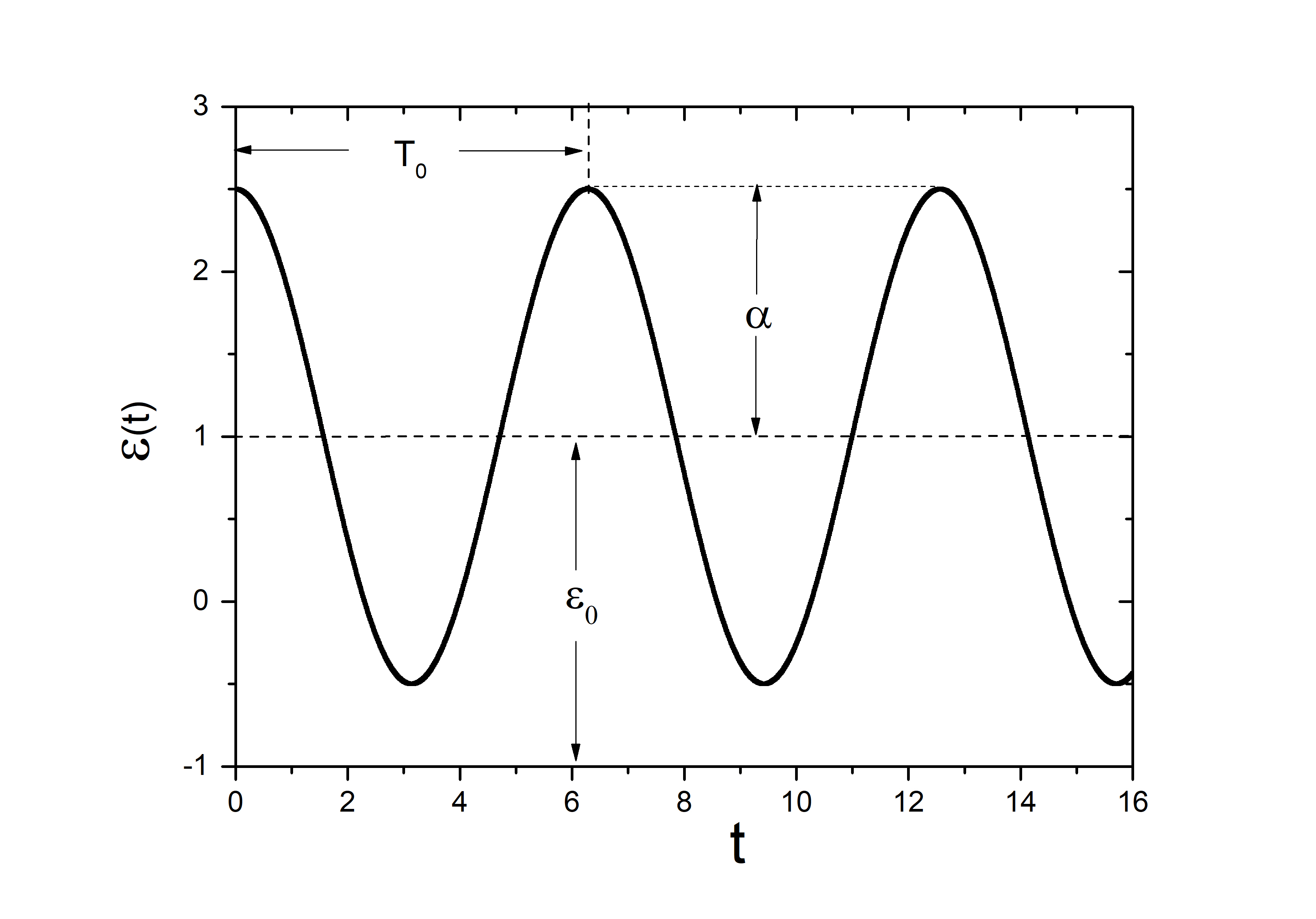
Figure 1: The periodically modulated coupling strength versus time, where $\alpha$, $\epsilon_{0}$, and $T_{0}$ are the modulation amplitude, average coupling strength, modulation period of the coupling term.

II III. Results

II.1 A. Coupled Stuart-Landau oscillators

In order to observe the effects of the periodically modulated coupling on the AD dynamics, let’s firstly consider the coupled nonidentical Stuart-Landau oscillators whose dynamics can be described as $\dot{Z_{i}}(t)=[1+j\omega_{i}-|Z_{i}(t)|^{2}]Z_{i}(t)$, where $Z_{i}(t)=x_{i}(t)+jy_{i}(t)$, $i=1,2$,$j=\sqrt{-1}$, $\omega_{i}$ is the intrinsic frequency of oscillator $i$. Without coupling ($\epsilon_{0}=0$), each oscillator has an unstable focus at the origin $|Z_{i}|=0$ and an attracting limit cycle with a oscillating frequency $\omega_{i}$. Considering the coupling scheme $\Gamma=\left[\begin{matrix}1&0\\ 0&1\end{matrix}\right]$ , AD can be stabilized in two coupled oscillators in Eq. I with frequency mismatches $\Delta\omega=|\omega_{2}-\omega_{1}|$ for constant coupling strength ($\alpha=0$) and $\omega_{1}=2$. The results aro indicate that the AD domain is bounded in the interval of coupling strength for given frequency mismatches while keeps stable when the frequency mismatch is larger than a critical value for given coupling strength as shown in Fig. 3(a). Since the modulated coupling strength has three control parameters, i.e. average coupling strength $\epsilon_{0}$, modulation frequency $\omega_{0}$, and modulation amplitude $\alpha$. Let’s firstly explore the effects of the modulation amplitude on AD with the modulation frequency $\omega_{0}=4$ fixed, and the average coupling strength $\epsilon_{0}=7.0$. Figs. 2(a)-(d) present the bifurcation diagram of $x_{1}$ for $\alpha=0.0,0.8,1.0,1.8$, respectively. For $\alpha=0$, the coupling strength is constant, and the coupled system transits to AD from the oscillating state (i.e. the time series of $x_{1}(t)$ display periodic oscillation for $\Delta\omega=2.0$ in Fig. 2(a)) when the frequency mismatch increases from zero to the value larger than $\Delta\omega_{c}=7.3$. As $\alpha=0.8$, the critical value of $\Delta\omega_{c}$ for AD becomes $5.6$ which is less than that of the constant coupling strength. The AD state is displayed by the time series of $x_{1}(t)$ in the insets of Fig. 2(b) for $\Delta\omega=6$. The coupled system has two intervals of AD domain $\Delta\omega\in[4.6,7.1]$ and $\Delta\omega\in[9.85,20]$ as $\alpha=1.0$. Then, three disconnected interval of AD domain along the direction of $\Delta\omega$ are observed as $\Delta\omega\in[1.1,1.2]$, $\Delta\omega\in[15.1,16.0]$, $\Delta\omega\in[18.3,20]$ for $\alpha=1.8$. The oscillating state is in periodic 2 for $\Delta\omega=8$ and $\alpha=1.0$ and in multi-period state for $\Delta\omega=5$ and $\alpha=1.8$ as shown in the insets of Figs. 2(c)(d),respectively.

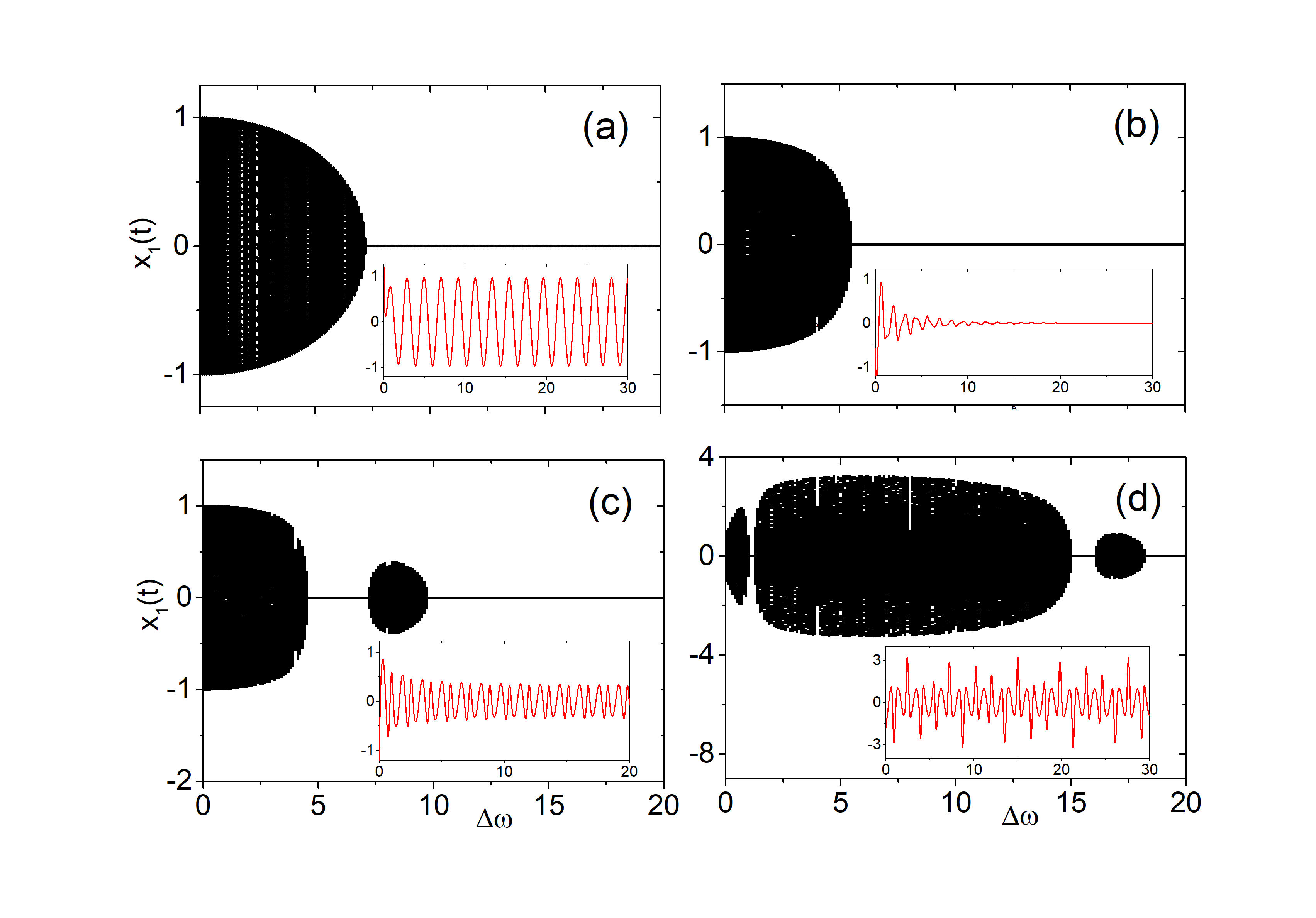
Figure 2: (Color online) The bifurcation diagram of $x_{1}$ (gray dots) versus frequency mismatch $\Delta\omega$ for $\epsilon_{0}=7$ and (a) $\alpha=0.0$, (b) $\alpha=0.8$, (c)$\alpha=1.0$, (d) $\alpha=1.8$, respectively. The insets are the time series of $x_{1}(t)$ for (a) $\alpha=0.0$,$\Delta\omega=2$, (b)$\alpha=0.8$, $\Delta\omega=6$, (c) $\alpha=1.0$, $\Delta\omega=8$ (d)$\alpha=1.8$, $\Delta\omega=5$.

To integrally figure out how the periodically modulated coupling influences the AD domain of the coupling oscillators, it is natural to reveal the mechanical regimes of the stabilities of AD under the periodically modulated coupling. Generally the stability of the AD domain in coupled oscillators is obtained from linear stability analysis of Eq. I around $Z_{i}=0$ if the coupling strength is constant. The characteristic eigenvalue is aro

$$\lambda_{1,2,3,4} = 1-\epsilon\pm\sqrt{\epsilon^{2}-\frac{(\omega_{2}-\omega_{1})^{2}}{4}}\pm j\frac{(\omega_{1}+\omega_{2})}{2},$$ (3)

then the AD domain is determined by $Re(\lambda)<0$, that is, $1\leq\epsilon\leq\Delta\omega/2$ and $\Delta\omega/2<\epsilon<1/2+\ \Delta\omega^{2}/8$ which is right the boundary lines of the AD domain as shown in Fig. 3(a). However, when $\epsilon$ is varying with time, the linear stability analysis around the original fixed points is not available any more. We numerically record the AD domain in parameter space $\Delta\omega$ versus $\epsilon_{0}$ (both are in the range of [0,20]) for a given $\omega_{0}=4.0$, and $\alpha=0,0.5,1.0,1.1,1.4,1.8$ as shown in Figs. 3(a)-(f), respectively. When the parameters of the coupled oscillators are in the blue (red) area, the oscillators are in AD (oscillating) states. With the increment of the modulation amplitude $\alpha$, the AD domain firstly expands by decreasing the critical frequency mismatches, which is the lower boundary of the AD domain for given average coupling strength $\epsilon_{0}$. Then the AD domain shrinks with the increment of $\alpha$ when $\alpha$ is larger than a critical value $\alpha_{c}$. Moreover, the AD domains split into two parts when $\alpha>1$ (it is repulsively coupled in some interval of each period) leading to a kind of ragged AD along the direction of frequency mismatch $\Delta\omega$. It should be emphasized that the AD is firstly observed to be ragged in the direction of parameter space $\Delta\omega$, as a comparison, OD domain is ragged in the direction of parameter space $\epsilon$ in the coupled system with a certain spatial frequency distribution ma . There are two segments of AD domains in parameter space of $\Delta\omega$ versus $\epsilon_{0}$, as an example, AD state occurs in the intervals of $\Delta\omega\in[3.6,5.4]$ and $\Delta\omega\in[9.3,20]$ as $\alpha=1.1$ and $\epsilon_{0}=5$, which can be also seen from the vertical line in Fig. 3(d). The two ragged AD domains keep shrinking and leaving away from each other with the increment of the modulation amplitude $\alpha$. Meanwhile, for a given $\alpha=1.5$, we explore the effects of the modulation frequency $\omega_{0}$ by numerically plotting the phase diagram in parameter space $\Delta\omega$ versus $\epsilon_{0}$ for $\omega_{0}=1,5,10,13,16,19$ in Figs. 4(a)-(f), respectively. The results show that the increment of the modulation frequency $\omega_{0}$ firstly splits the AD domain into two parts with the upper one larger than the lower one, then the lower larger one expands while the upper larger one shrinks. Finally, the two parts merged into one large AD domain again. To present detailed insight of the effects of $\alpha$ on the AD domain, the normalized ratio factor $R=S(\alpha)/S(\alpha=0)$ is defined to qualify the change of AD domains under designated regions ($\epsilon_{0}\in[0,20]$ and $\delta\omega\in[0,20]$) in Fig. 5(a) where the modulation frequency $\omega_{0}=3,5,10,15,20$, respectively. $S(\alpha)$ is the area of the AD domains for given $\alpha$ while $S(\alpha=0$) represents the area of AD domains for $\alpha=0$ (i.e., the red domains in Fig. 3(a)).

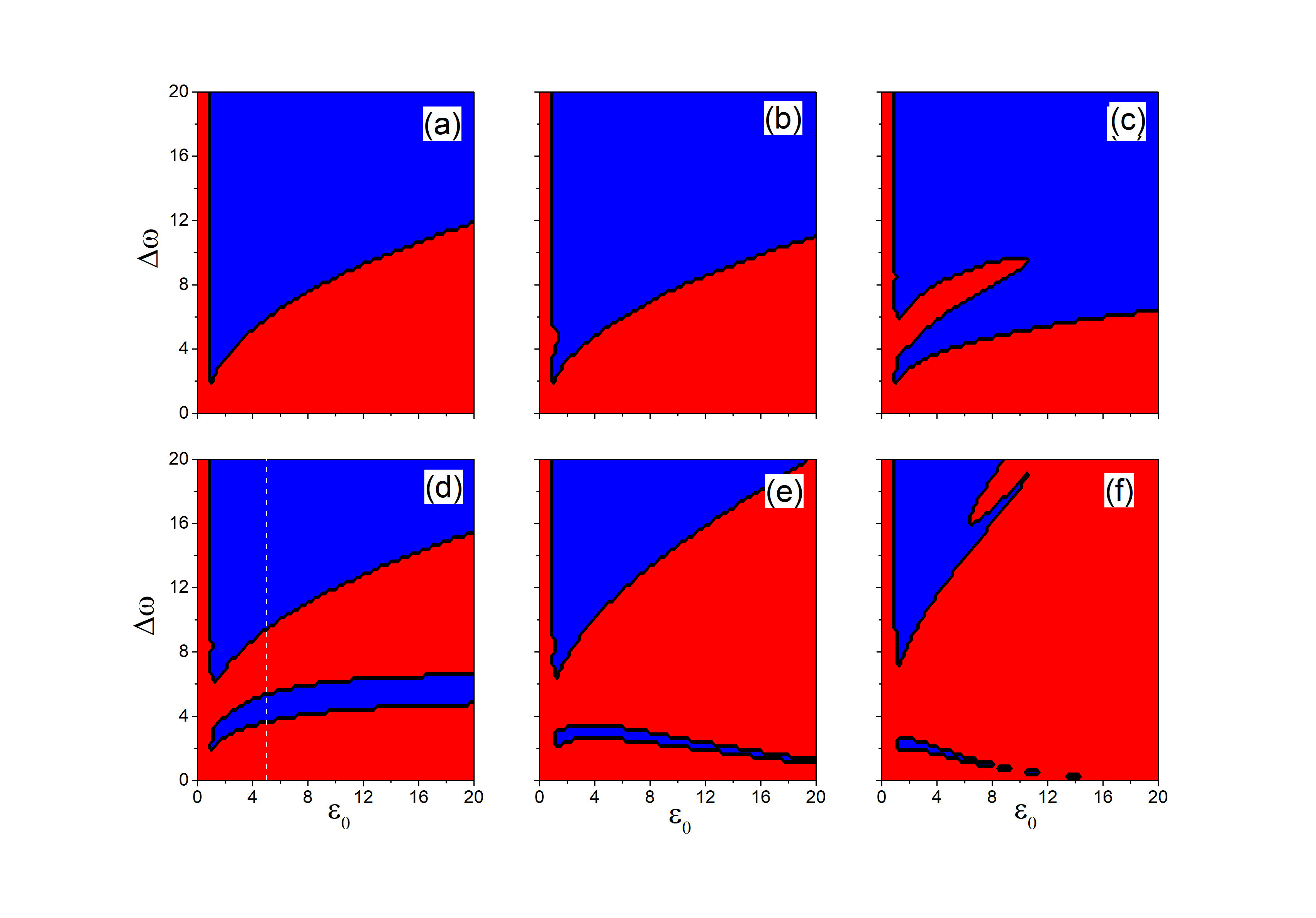
Figure 3: (color online) The phase diagram of the parameters $\alpha$ versus $\Delta\omega$ for $\omega_{0}=4.0$ and (a) $\alpha=0.0$, (b) $\alpha=0.5$, (c) $\alpha=1.0$, (d) $\alpha=1.1$, (e) $\alpha=1.4$, (f) $\alpha=1.8$, respectively. Where the blue domains are in AD states and the red domains are the oscillating states.

It is obvious that the ratio $R$ firstly increases slightly (expansion of AD domain) and then decreases sharply to small value (reduction of AD domain) as $\alpha$ increases from 0 to 2 for all modulation frequencies $\omega_{0}$. There is a critical value $\alpha_{c}$ with which the AD domain gets to the largest value for each given modulation frequency $\omega_{0}$. That is to say there is an optimal modulation amplitude of the coupling strength with which the coupled system has the largest AD domain. When $\alpha<\alpha_{c}$, the increment of $\alpha$ tends to enlarge the area of AD domain by shrinking that of the oscillating domain, otherwise, the AD domain is torn into multi domains by the birth of oscillating domain and shrinks with the increment of modulation amplitude $\alpha$. Interestingly, the optimal value of $\alpha_{c}$ increases with the increment of the modulation frequency $\omega_{0}$ as shown the inset in Fig. 4(a). The larger the modulation frequency $\omega$ is, the larger the modulation amplitude is needed to maximize the AD domain.

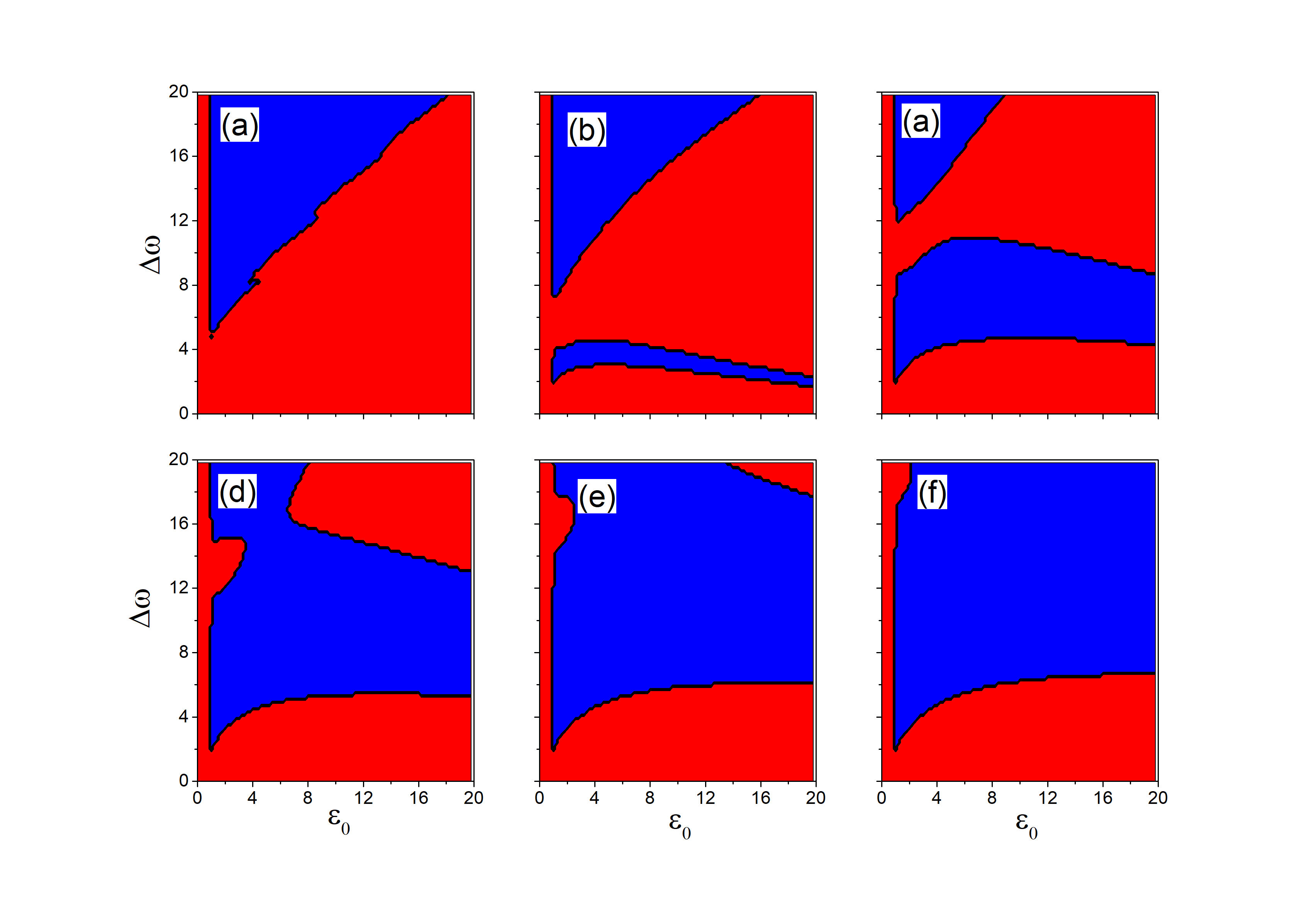
Figure 4: (color online) The phase diagram of the parameters $\Delta\omega$ versus $\epsilon_{0}$ for $\alpha=1.4$ and (a) $\omega_{0}=1.0$, (b) $\omega_{0}=5$, (c) $\omega_{0}=10$, (d) $\omega_{0}=13$, (e) $\omega_{0}=16$, (f) $\omega_{0}=19$, respectively. Where the blue domains are in AD states and the red domains are the oscillating states.

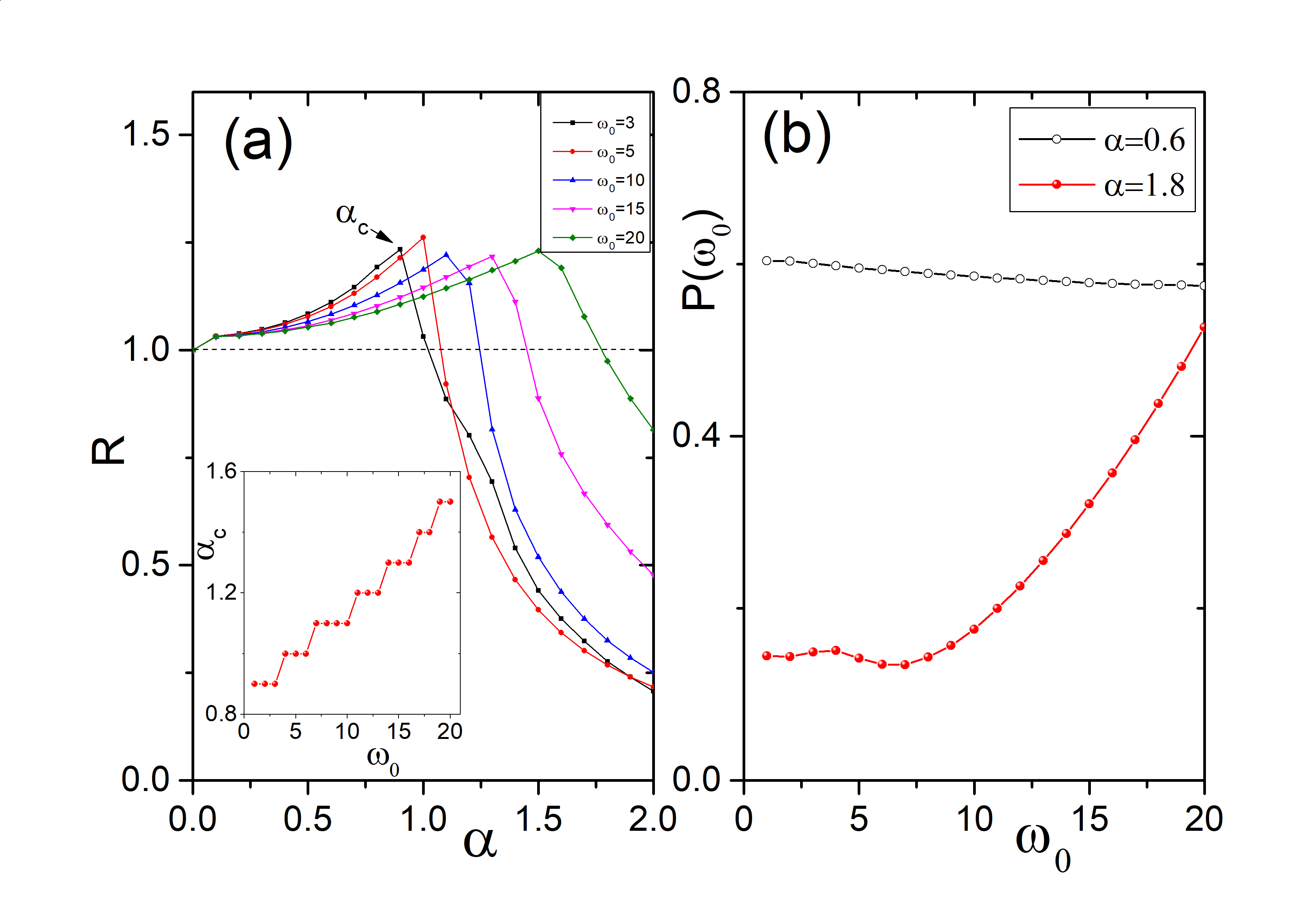
Figure 5: (color online) (a) The ratio $R$ defined in the context versus $\alpha$ for $\omega_{0}=3,5,10,15,20$, respectively. The inset presents the critical value $\alpha_{c}$ versus the modulation frequency $\omega_{0}$, where $\alpha_{c}$ is the value when $R$ gets the maximum (the coupled oscillators have largest AD domains in parameter space $(\epsilon_{0},\Delta\omega))$ (b) The proportion $P(\omega_{0})$ of AD states versus $\omega_{0}$ for a given $\alpha=0.6$ (black hollow-dotted line),$\alpha=1.8$ (red solid-dotted line), respectively.

Now let’s focus on the effects of the modulation frequency $\omega_{0}$ on the AD domain. Define the proportion of the AD domain on the designated regions $\epsilon_{0}\in[0,20]$ and $\delta\omega\in[0,20]$ as $P(\omega_{0})=S(\omega_{0})/S_{tot}$ for given $\omega_{0}$, where $S(\omega_{0})$ is the area of the AD domain for given $\omega_{0}$, and $S_{tot}$ is the area of the designated region. Then $P(\omega_{0})$ versus the modulation frequency $\omega_{0}$ can be numerically presented for an arbitrarily given modulation amplitude $\alpha$. Figure. 5(b) presents the results of $P(\omega_{0})$ versus $\omega_{0}$ for given $\alpha=0.6,1.8$ respectively. $P(\omega_{0})$ linearly decreases with a slow speed for $\alpha=0.6$ while obviously increases for $\alpha=1.8$ as $\omega_{0}$ increase from 7 to 20. Therefore, the modulation frequency $\omega_{0}$ is beneficial to shrink AD domain for small modulation amplitude $\alpha$, otherwise, the AD domain expands quickly with the increment of the modulation frequency $\omega_{0}$ as $\alpha$ is large (larger than the maximal $\alpha_{c}$.

II.2 B. Coupled Rossler oscillators

AD can also be observed in coupled chaotic oscillators with time delay coupling pra , and on-off coupling schemes sun . It is nature to explore the effects of the periodically modulated coupling on the AD domain in coupled chaotic nonidentical oscillators. Let’s consider the coupled chaotic Rossler oscillators with two different time scales.

$$\dot{x_{i}}(t) = -\omega_{i}(y_{i}(t)+z_{i}(t)),$$

$$\dot{y_{i}}(t) = \omega_{i}(x_{i}(t)+ay_{i}(t)),$$

$$\dot{z_{i}}(t) = \omega_{i}(b+z_{i}(t)(x_{i}(t)-c).$$ (4)

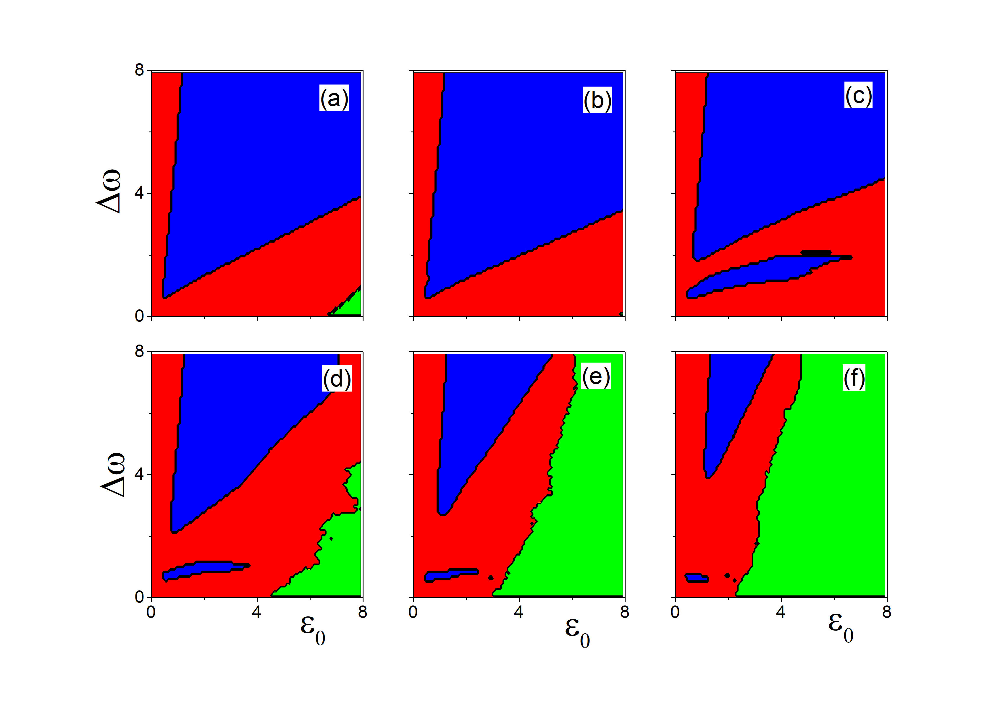
Figure 6: (color online) The phase diagram of the parameters $\Delta\omega$ versus $\epsilon_{0}$ in coupled Rossler oscillators for (a) $\alpha=0.0$, (b) $\alpha=0.5$, (c) $\alpha=1.0$, (d) $\alpha=1.2$, (e) $\alpha=1.4$, (f) $\alpha=1.6$, respectively, where the blue domain is AD state, the red domain is the oscillating state, and the blue domain is the blowup state.

where $\omega_{i}$ rescales the rolling speed of single chaotic oscillator. The single uncoupled oscillator is in chaotic regime for given parameters $a=0.15$, $b=0.4$, $c=8.5$, and has an unstable fixed point $(-ay^{*},-z^{*},z^{*})$ with $z^{*}=(c-\sqrt{c^{2}-4ab})/(2a)$. $\omega_{1}$ is arbitrarily set to 2 , and the frequency mismatch of two coupled oscillators is $\Delta\omega=|\omega_{1}-\omega_{2}|$. The periodically modulated coupling term $\epsilon(t)$ is the same as Eq. 2 with the modulation frequency $\omega_{0}=1$. The coupling scheme is set as $\Gamma=\left[\begin{matrix}1&0&0\\ 0&0&0\\ 0&0&0\end{matrix}\right]$, (i.e. the interacting variable is $x(t)$). Then the AD domain with different periodic coupling strength can be conveniently observed by presenting the phase diagram of parameters $\Delta\omega$ versus $\epsilon_{0}$ for $\alpha=0,0.5,1.0,1.2,1.4,1.6$ as shown in Figs. 6(a)-(f), respectively. With constant coupling strength ($\alpha=0$), the coupled Rossler oscillator has three states, AD state (v-shaped blue domain), oscillating state (red domain), and blowup to infinite (green domain). As $\alpha=0.5$ the AD domain is enlarged while the domain of blowup state is shrunk. Then the AD domain is ragged into two parts as $\alpha$ is larger than $1.0$. Finally, the AD domain shrinks while the domain of the blowup state occurs again and keeps enlarging as $\alpha$ increases from $1.2$ to $2.0$.

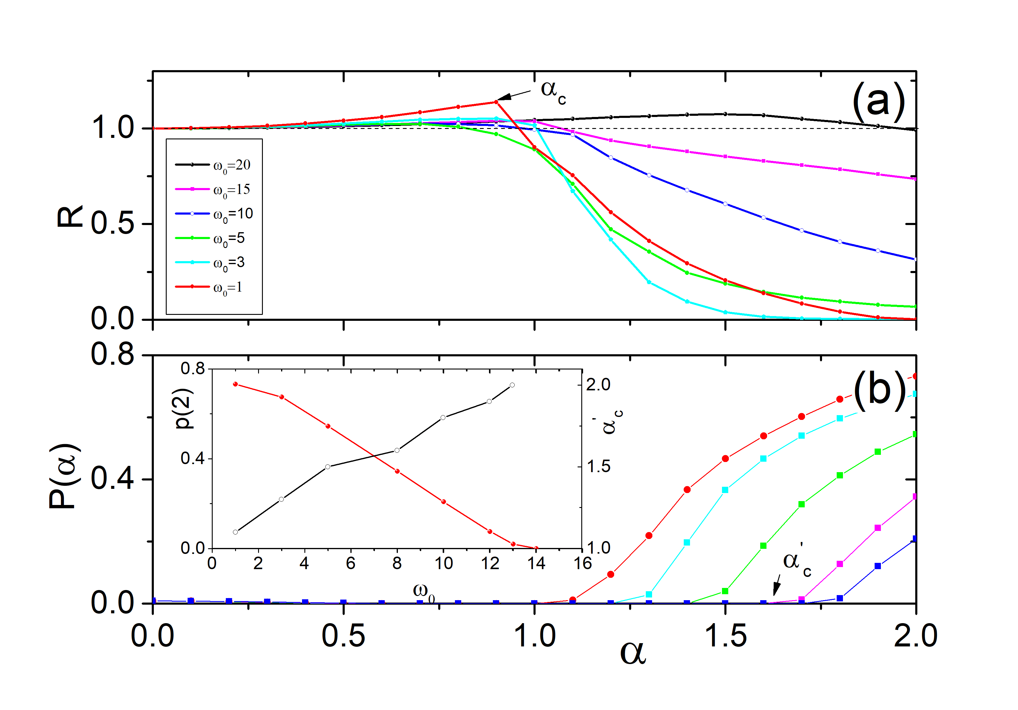
Figure 7: (color online) (a) The ratio $R$ defined in the context versus $\alpha$ for $\omega_{0}=1,3,5,10,15,20$, respectively. (b) The proportion $P(\alpha)$ of blowup domains versus $\alpha$ for given $\omega_{0}=1$ (red line), $\omega_{0}=3$ (cyan line), $\omega_{0}=5$ (green line), $\omega_{0}=8$ (magenta line), $\omega_{0}=10$ (blue line), respectively. The red solid dotted line in inset is the proportion of $P(\alpha=2)$ versus $\omega_{0}$, and the black hollow dotted line in inset is the critical value of $\alpha^{\prime}_{c}$, where $\alpha^{\prime}_{c}$ is the critical value when $p(\alpha)>0$.

Figure. 7(a) exhibits the change of areas of AD domain by the ratio factor $R$ versus the modulation amplitude $\alpha$ for given modulation frequency $\omega_{0}=1,3,5,10,15,20$, respectively. Where the ratio factor $R$ is defined the same as the above one with the designated region of $(\epsilon,\Delta\omega)$ space in the range of $\epsilon\in[0,8]$ and $\Delta\omega\in[0,8]$. The effects of the modulation frequency and modulation amplitude of the coupling strength on AD domains in coupled Rossler oscillators are similar to that in the coupled Stuart-Landau oscillators. The increment of the modulation amplitude tends to enlarge the AD domain first then shrinks the AD domain for a given modulation frequency $\omega_{0}$. There is also a critical value $\alpha_{c}$ with which the coupled Rossler oscillators have the largest AD domain. Similarly, we may defined the proportion of blowup domain as $P(\alpha)=S(\alpha)/S_{tot}$ for given $\alpha$, where $S(\alpha)$ is the area of parameter space of blowup domain and $S_{tot}$ is the area of domain in the designated area of $\epsilon\in[0,8]$ and $\Delta\omega\in[0,8]$. Then the effects of $\alpha$ on blowup can be indicated by $P(\alpha)$ versus $\alpha$ as shown in Fig. 7(b) for given $\omega_{0}=1,3,5,8,10$, respectively. It is obvious that $P(\alpha)$ is small and approaches to zero for small $\alpha$ and then grow up again when $\alpha$ is larger than a critical value $\alpha^{\prime}_{c}$. The critical value $\alpha^{\prime}_{c}$ increases linearly with the increment of the modulation frequency $\omega_{0}$ as shown the inset in Fig. 7(b). Meanwhile, the increment of $\omega_{0}$ tends to decrease linearly the area of blowup domain according to the relationship between $p(2)$ versus $\omega_{0}$ for given $\alpha=2$ as shown the red solid-dotted line in the inset of Fig.7(b).

III IV. MECHANISM ANALYSIS

Since the modulated coupling strength varies with time, the linear stability analysis near the fixed points is not available to predict the dynamics regimes. Based on the fact that the conditional Lyapunov exponent pyr is a valid tool to determine the generalized synchronization, it is expected to determine the stability of the AD state in the coupled nonidentical oscillators. Let $\delta z_{i}=z_{i}-z^{*}_{i},(i=1,2)$ be an infinitesimal perturbation added to oscillator $i$, then whether the perturbed trajectories of Eq. I could be converged to the fixed point $z^{*}$ is mainly determined by the set of variational equations

$$\left[\begin{matrix}\dot{\delta z_{1}}(t)\\ \dot{\delta z_{2}}(t)\end{matrix}\right]=\left[\begin{matrix}(DF_{1}(z^{*}_{1}))&0\\ 0&DF_{2}(z^{*}_{2})\end{matrix}\right]\left[\begin{matrix}\delta z_{1}(t)\\ \delta z_{2}(t)\\ \end{matrix}\right]+\epsilon(t)\Gamma A\left[\begin{matrix}\delta z_{1}(t)\\ \delta z_{2}(t)\\ \end{matrix}\right]$$ (5)

Here $z^{*}_{1}=(0,0)$, $z^{*}_{2}=(0,0)$ are the original fixed points of single oscillators. $DF_{1}()$ and $DF_{2}()$ are the deviations of the two coupled oscillators. $\Gamma$ is the the coupling scheme ($\Gamma=\left[\begin{matrix}1&0\\ 0&1\end{matrix}\right]$ for coupled LS oscillators) and $A=\left[\begin{matrix}-1&1\\ 1&-1\end{matrix}\right]$ is the link matrix whose eigenvalue is $\lambda_{1}=0$ and $\lambda_{2}=-2$. Solving Eq. 5 numerically for $\lambda_{2}=-2$, we are able to obtain the conditional Lyapunov exponent $\lambda_{c}$ with respect to the parameters of the coupling strength and frequency mismatches, based on which the stable domain of AD, i.e. the domain with $\lambda_{c}<0$, can be identified. In Figs. 8(a)-(d), we plot the conditional Lyapunov exponent $\lambda_{c}$ as a function of $\Delta\omega$ for $\epsilon_{0}=7$, and $\alpha=0.0,0.8,1.0,1.8$, respectively. The conditional Lyapunov exponent transit to negative from positive when coupled system transit from oscillating state to AD state which matches well with the bifurcation results in grey dots.

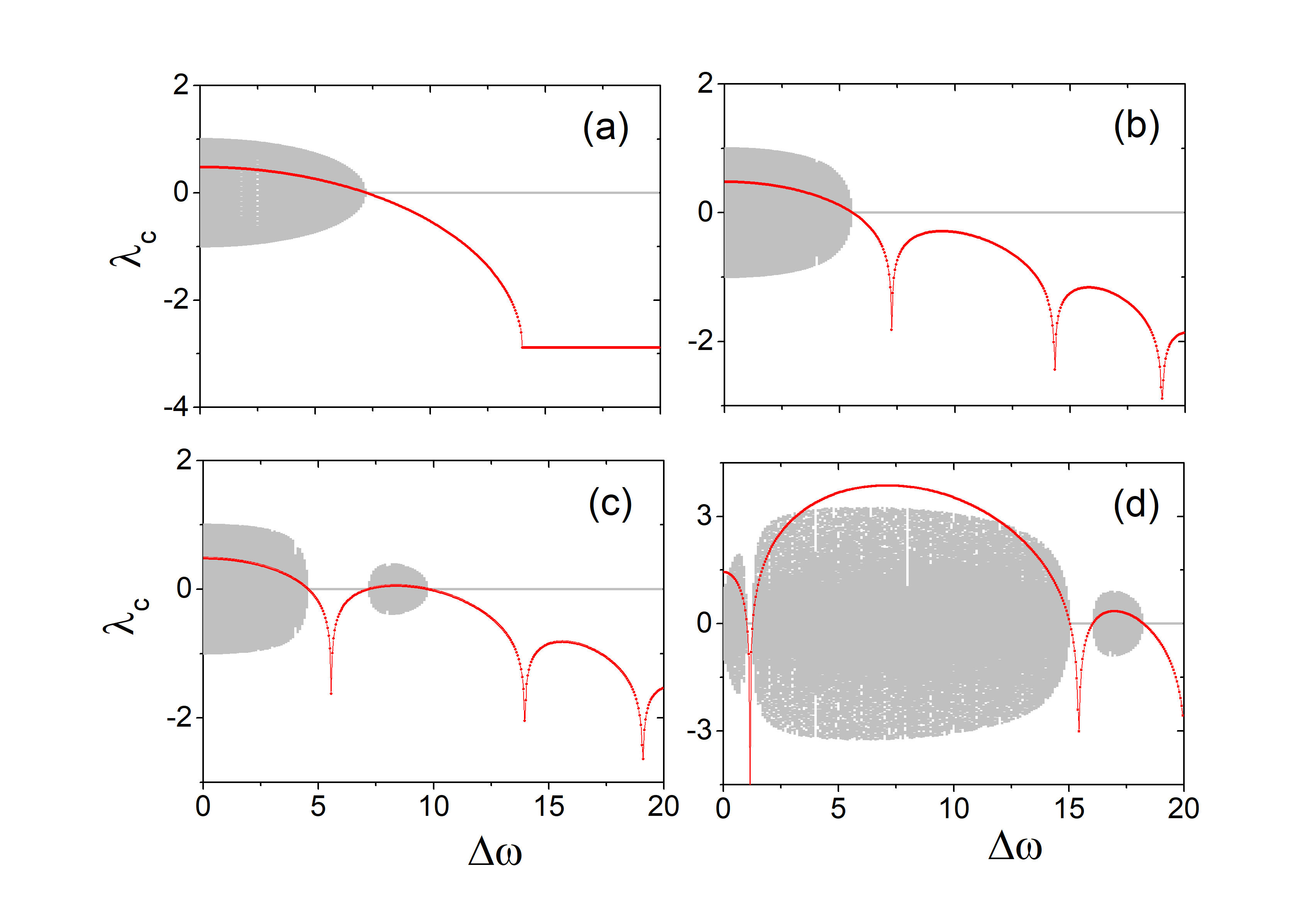
Figure 8: (color online) The conditional Lyapunov exponent $\lambda_{c}$ versus $\Delta\omega$ for $\epsilon=7$, $\omega_{0}=4$ and (a) $\alpha=0.0$, (b) $\alpha=0.8$, (c)$\alpha=1.0$, (d) $\alpha=1.8$, respectively. The grey dots are bifurcation diagram.

To observe clearly how the varying coupling strength influences the dynamical of the coupled oscillators, the phase diagrams of $x_{1}(t)$ versus $y_{1}(t)$ for $\Delta\omega=4.5$ (AD state in numerical results), and $\Delta\omega=6.5$ (oscillating state in numerical results) are presented in Figs. 9(a)(b), respectively. The value of the normalized coupling strength ($\epsilon(t)/\epsilon_{0}$) is indicated by the color of the phase diagram. Fig. 9(a) indicates that the oscillator may leave away from (stage AB) or approach to (stage BC) the original fixed point ($0,0$) in each period of the modulated coupling strength. The speed of approaching to the original fixed point is larger than that of leaving away which results to that the coupled system approaches to the fixed points gradually as time goes to infinite. The enlarged diagram indicates that the coupled system may leave away from the original point in some interval of each period of the modulated coupling after approaching to the fixed point. Therefore, the oscillator will never stay on the original fixed point no matter how near it approach to the original fixed point (in this sense, the original fixed point is not stable). However, owing to the finite preciseness of the computer, AD can be observed in the numerical results when the distance between the oscillator and the original fixed point is smaller than the computer’s preciseness. In Fig. 9(b), the oscillator may also diverge from (stage DE) and approach to (stage EF) the original fixed point in each period of the modulated coupling. Noted that the speed of approaching to fixed point is larger than that of diverging from the fixed point, however, the time of the former one is shorter than the later one. As a result, the coupled oscillator forms an oscillating state. The speed of approaching to or leaving away from the fixed point is related to the value of the local conditional Lyapunov exponent pik1 as shown in Figs. 9(c)(d), respectively. Positive local conditional Lyapunov exponent makes the oscillator leave away from the fixed point while negative one drive the coupled system to converge to the fixed point. The speed of approaching to or diverging from the fixed point is related to the absolute value of the local conditional Lyapunov exponent. Compared the results between Fig. 9(c) and Fig. 9(d), the final fate of the coupled oscillator is completely determined by the average value of the local conditional Lyapunov exponent in one modulation period. The coupled system is in AD state if the average value of the local conditional Lyapunov exponent is negative, otherwise it is in oscillating state. The conditional Lyapunov exponent is also available to predict the AD dynamics in the coupled Rossler oscillators. Figs. 10(a)-(d) present the conditional Lyapunov exponent together with the bifurcation diagram on variable $x_{1}$ versus $\Delta\omega$. The conditional Lyapunov exponent gets to negative value when the coupled Rossler oscillators experience AD which also agrees well with the bifurcation diagram.

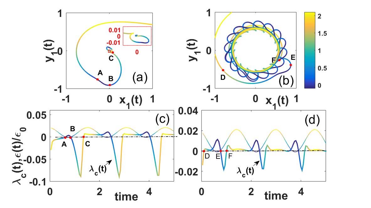
Figure 9: (color online) (a) The phase diagram of $y_{1}(t)$ versus $x_{1}(t)$ for $\alpha=1.1$, $\epsilon=5$, $\Delta\omega=4.5$. The inset is the enlarged part of the red squared area. A,B,C note the position when the local conditional Lyapunov exponent $\lambda_{c}(t)$ is crossing $x$ axis as shown in Fig. 9(c). The colors of lines in the Fig. 9 denote the values of the normalized coupling strength $\epsilon(t)/\epsilon_{0}$. (b) The phase diagram of $y_{1}(t)$ versus $x_{1}(t)$ for $\alpha=1.1$, $\epsilon=5$, $\Delta\omega=6.5$. D,E,F note the position when the local conditional Lyapunov exponent $\lambda_{c}(t)$ is crossing $x$ axis as shown in Fig. 9(d). The local conditional Lyapunov exponent and the normalized coupling strength ($1\%$ of $\epsilon(t)/\epsilon_{0}$) versus time for (c) $\Delta\omega=4.5$ and (d) $\Delta\omega=6.5$

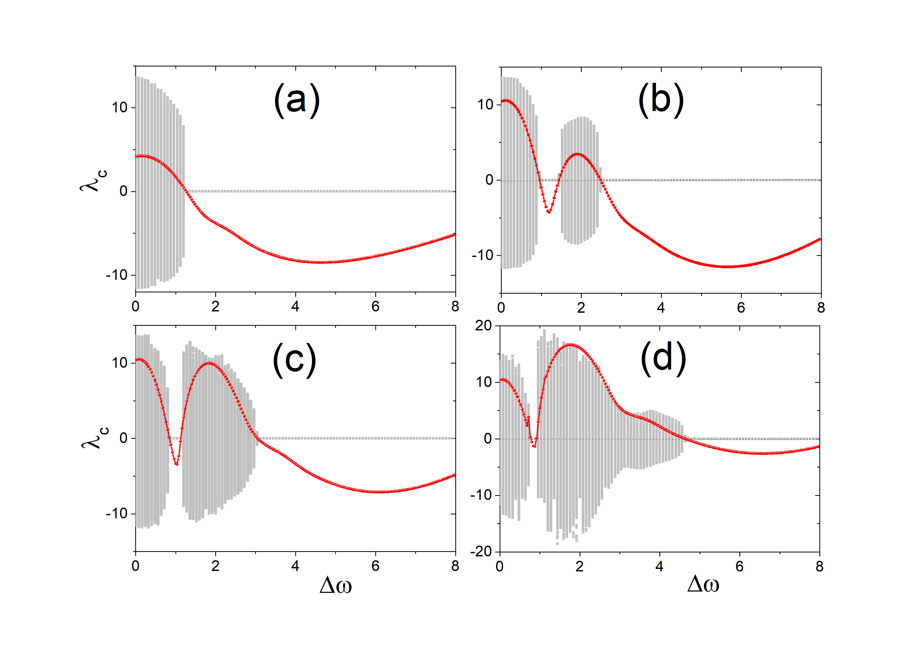
Figure 10: (color online) The conditional Lyapunov exponent $\lambda_{c}$ (red lines) versus $\Delta\omega$ for $\epsilon=2$ and (a) $\alpha=0.5$, (b) $\alpha=1.0$, (c)$\alpha=1.2$, (d) $\alpha=1.4$, respectively in the coupled Rossler oscillators (the conditional Lyapunov exponent is magnified 50 times for the convenience of observation in the figure). The grey dots are bifurcation diagram.

To verify the stability of the fixed points further, we add the noise on the coupled system,

$$\dot{X_{1}}(t) = f_{1}(X_{1}(t))+\epsilon(t)\Gamma(X_{2}(t)-X_{1}(t))+\xi_{1}(t),$$

$$\dot{X_{2}}(t) = f_{2}(X_{2}(t))+\epsilon(t)\Gamma(X_{1}(t)-X_{2}(t))+\xi_{2}(t),$$ (6)

where the independent stochastic variables $\xi_{i}(t)$ are the zero-mean white Gauss noises with strength $\sigma$, namely, $<\xi_{i}(t)>=0$,$<\xi_{i}(t)\xi_{j}(t^{\prime})>=2\sigma\delta(t-t^{\prime})\delta_{ij}$,$\gamma$ is the same as the above. If the stability of AD is strong, then the periodically modulated coupled system with noise may meander in the vicinity of fixed point. Define the variable $\gamma$ as the ability of resisting noise as following,

$$\gamma=\left\{\begin{array}[]{lr}50,&\eta>=20,\\ 40,&15\leq\eta<20\\ 30,&10\leq\eta<15\\ 20,&2\leq\eta<10\\ 10,&\eta<2,\end{array}\right.$$ (7)

where $\eta=max(x_{1}-x^{*}_{1})/\sigma$ is the ratio of the maximum $x_{1}(t)-x^{*}_{1}$ to the noise strength $\sigma$. Then AD is more stable if $\eta$ is smaller. The phase diagram of $\gamma$ in the parameter $\Delta\omega$ versus $\epsilon_{0}$ of coupled LS oscillators are presented in Figs. 10 (a)-(b) for $\alpha=1.1$, and $\omega_{0}=4$, as well as that of coupled Rossler oscillators presented in Figs. 10 (c)-(d) for $\alpha=1.0$, and $\omega_{0}=1$. According to Figs. 10(a)(b), it is easy to conclude that the ragged AD domain in the upper part (except the edge parts) has stronger stability than that in the lower part. Noticed that the upper part of the ragged AD domain is stable for constant coupling strength (without modulation) while the lower AD domain is newly born by the modulated coupling which has less stability than the original AD domain. Moreover, the conclusion is slightly influenced by the noise intensity.

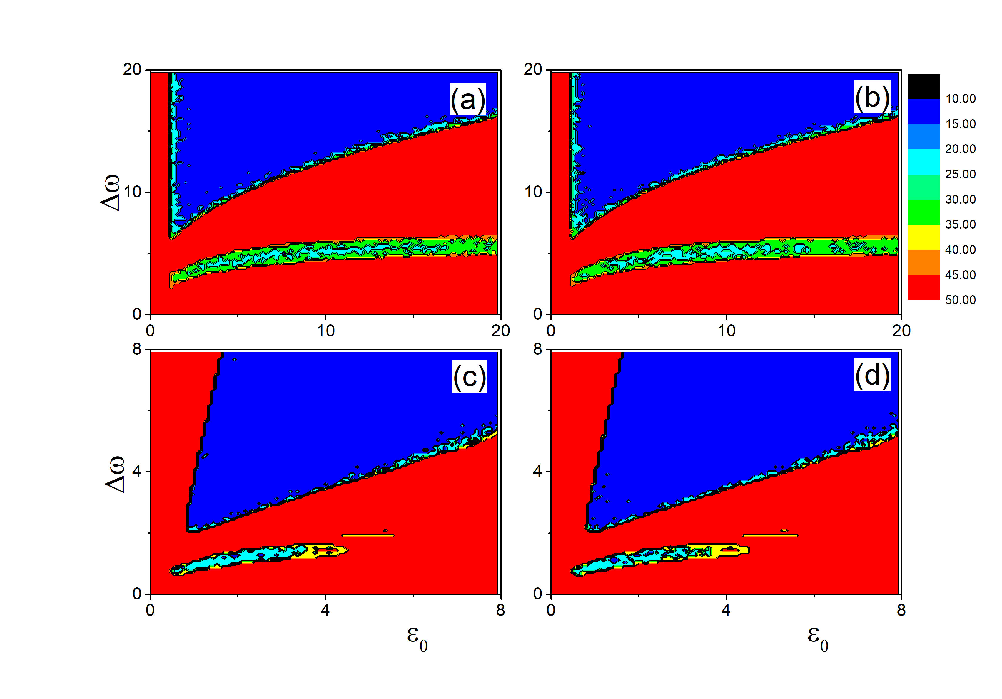
Figure 11: The phase diagram of the parameters $\Delta\omega$ versus $\epsilon_{0}$ with noise strength being (a) $\sigma=0.001$ in coupled $SL$ oscillators, (b) $\sigma=0.1$ in coupled SL oscillator,(c) $\sigma=0.001$ in coupled Rossler oscillators, (d) $\sigma=0.1$ in coupled Rossler oscillators. The colorbar determines the values of $\gamma$ in Eq. 7.

V. Conclusions

Totally, both the modulation frequency and the modulation amplitude of the periodically modulated coupling strength significantly influenced the dynamics of the coupled limit cycles or chaotic oscillators. The increment of the modulation amplitude firstly increases the AD domain and then decreases the AD domain as it is larger than a critical value which is related to the modulation frequency. That is to say, small modulation amplitude of the coupling strength is helpful to enlarge the AD domain of the coupled nonidentical oscillators. However, when the coupling term is varying between repulsive (negative) and attractive (positive), the AD domains may be shrunk and ragged to several parts by the occurrence of oscillating domain. Meanwhile, the increment of modulation frequency of the periodic coupling tends to slightly decrease the AD domains for small modulation amplitude while dramatically increase the AD domains for large modulation amplitude. According to the local conditional Lyapunov exponent of the periodically coupled oscillators, one may find that the stability of the AD states is varying with the coupling strength. Whether the coupled oscillators can converge to AD state or not is completely determined by the sign of the averaged conditional Lyapunov exponent. The periodically modulated coupling is beneficial to realize AD and is more easy to physical realization than on-off coupling which needs high speed stitchers and is difficult to apply, therefore, it has potential application in the dynamical control in engineering.

Acknowledgement Weiqing Liu is supported by the National Natural Science Foundation of China (Grant No. 11765008) and the Qingjiang Program of Jiangxi University of Science and Technology. Jiangnan Chen is supported by the Project of Jiangxi province.

Reference

References

- (1) Z. Sun,N. Zhao , X. Yang ,W. Xu, Nonlinear Dyn, 92,(3) 1185-1195 (2018).
- (2) Y. Kuramoto, Chemical Oscillations, Waves, and Turbulence (Springer, Berlin, 1984).
- (3) A. Pikovsky, M. Rosenblum, and J. Kurths, Synchronization: A Universal Concept in Nonlinear Sciences (Cambridge University Press, Cambridge, 2001).
- (4) G. Song , N. V. Buck and B. N. Agrawal, J. Guid Control Dyn., 22 (1999) 4330.
- (5) A. Koseska, E. Ullner, E. Volkov, J. Kurths, and J. Garcia-Ojalvo, J. Theor. Biol. 263, 189 (2010).
- (6) E. Ullner , A. Zaikin, E. I. Volkov and J. Garcia- Ojalvo, Phys. Rev. Lett., 99 148103 (2007).
- (7) M. Y. Kim , R. Roy, J. L. Aron,T. W. Carr and I. B. Schwartz, Phys. Rev. Lett., 94 088101 (2005).
- (8) A. Prasad, Y. Lai, A. Gavrielides and V. Kovanis , Phys. Lett. A, 318 (2003) 71.
- (9) G. Saxena, A. Prasad, and R. Ramaswamy, Phys. Rep. 521, 205 (2012).
- (10) A. Koseska ,E. Volkov and J. Kurths , Europ Lett., 85 28002(2009).
- (11) Y. Goto and K. Kaneko, Phys. Rev. E 88, 032718 (2013).
- (12) N. Suzuki, C. Furusawa, and K.Kaneko, PLoS ONE 6, e27232 (2011).
- (13) R. Curtu, Physica D 239, 504 (2010).
- (14) K. P. Zeyer, M. Mangold, and E. D. Gilles, J. Phys. Chem. 105, 7216 (2001).
- (15) A. Koseska, E. Volkov, and J. Kurths, Phys. Rev. Lett., 111 024103(2013).
- (16) W. Zou, D. V. Senthilkumar, A. Koseska, and J. Kurths, Phys. Rev. E 88, 050901(R) (2013).
- (17) A. Koseska, E. Volkov, and J. Kurths, Phys. Rep. 531, 173 (2013).
- (18) R. Herrero, M. Figueras, J. Rius, F. Pi, and G. Orriols, Phys. Rev. Lett., 84 5312 (2010).
- (19) D.G. Aronson, G.B. Erementrout, N. Kopell, Physica D 41, 403-449 (1990).
- (20) Y. Wu,W. Liu, J. Xiao, W. Zou, and J. Kurths, Phys. Rev. E 85, 056211 (2012).
- (21) A. Koseska, E. Volkov, and J. Kurths, Chaos 20, 023132 (2010).
- (22) G.B. Ermentrout, Physica D 41 219 (1990).
- (23) J. Yang., Phys. Rev. E 76 (2007) 016204.
- (24) L. Rubchinsky, M. Sushchik, Phys. Rev. E 62 6440 (2000).
- (25) F. M. Atay, Physica D 183 1 (2003).
- (26) Z. Hou and H. Xin, Phys. Rev. E 68 055103R (2003).
- (27) W. Liu, X. Wang, S. Guan, C.-H. Lai, New J. Phys. 11 093016 (2009).
- (28) A. Zakharova, M. Kapeller, and E. Scholl,Phys. Rev. Lett. 112, 154101 (2014 .
- (29) H. Bi, X. Hu, X. Zhang, Y. Zou, Z. Liu, and S. Guan, Europhys. Lett. 108, 50003 (2014).
- (30) N. Zhao, Z. Sun, X. Yang, and W. Xu, Phys. Rev. E 97, 062203 (2018).
- (31) U. K. Verma, A. Sharma, N. K. Kamal, J. Kurths, M. D. Shrimali, Scientific Reports 7 7936 (2017).
- (32) K. Konishi, Phys. Rev. E 68, 067202 (2003).
- (33) R. Karnatak, R. Ramaswamy, and A. Prasad, Phys. Rev. E 76, 035201(R) (2007).
- (34) A. Prasad, M. Dhamala, B. M. Adhikari, and R. Ramaswamy, Phys. Rev. E 81, 027201 (2010).
- (35) W., J. Xiao, L. Li, Y. Wu, M. Lu, Nonlinear Dyn 69:1041-1050(2012)
- (36) T. Banerjee and D. Ghosh, Phys. Rev. E 89, 052912(2014).
- (37) W. Liu, G. Xiao, Y. Zhu,etc., Phys. Rev. E 91, 052902 (2015).
- (38) Zou, W. Zhan, M., Phys. Rev. E 80, 065204 (2009).
- (39) W. Zou, D. V. Senthilkumar,J. Duan, J. Kurths, Phys. Rev. E 90, 032906 (2014).
- (40) A. Prasad,. Phys. Rev. E, 72, 056204 (2005).
- (41) L. Chen, C. Qiu, H. Huang, Phys. Rev. E 79, 045101 (2009).
- (42) A. Buscarino, M. Frasca, M. Branciforte, L. Fortuna, J. Sprott, Nonlinear Dyn. 88, 673-683 (2017).
- (43) M. Schroder, M. Mannattil, D. Dutta, S. Chakraborty, M. Timme, Phys. Rev. Lett. 115, 054101 (2015).
- (44) S. Li, N. Sun, L. Chen, and X. Wang, Phys. Rev. E 98, 012304 (2018).
- (45) A. Prasad,PRAMANA journal of physics 81(03) 0407-0415 (2013).
- (46) K. Suresh, M.D. Shrimali , Awadhesh Prasad, K. Thamilmaran, Physics Letters A 378 2845-2850 (2014)
- (47) H. Ma, W. Liu, Y. Wu, M. Zhan, J. Xiao, Communications in Nonlinear Science and Numerical Simulation 19(8) 2874-2882 (2014).
- (48) X. Sun, M. Perc, and J. Kurths, Chaos 27, 053113 (2017)
- (49) K. Pyragas, Phys. Rev. E 56(5) 5183 (1997)
- (50) A. Pikovsky, Chaos 3, 225 (1993).