The Relativistic Hopfield network: rigorous results
Abstract
The relativistic Hopfield model constitutes a generalization of the standard Hopfield model that is derived by the formal analogy between the statistical-mechanic framework embedding neural networks and the Lagrangian mechanics describing a fictitious single-particle motion in the space of the tuneable parameters of the network itself. In this analogy the cost-function of the Hopfield model plays as the standard kinetic-energy term and its related Mattis overlap (naturally bounded by one) plays as the velocity. The Hamiltonian of the relativisitc model, once Taylor-expanded, results in a -spin series with alternate signs: the attractive contributions enhance the information-storage capabilities of the network, while the repulsive contributions allow for an easier unlearning of spurious states, conferring overall more robustness to the system as a whole.
Here we do not deepen the information processing skills of this generalized Hopfield network, rather we focus on its statistical mechanical foundation. In particular, relying on Guerra’s interpolation techniques, we prove the existence of the infinite volume limit for the model free-energy and we give its explicit expression in terms of the Mattis overlaps. By extremizing the free energy over the latter we get the generalized self-consistent equations for these overlaps, as well as a picture of criticality that is further corroborated by a fluctuation analysis.
These findings are in full agreement with the available previous results.
I Introduction: a glance at the relativistic Hopfield network
Recent advances, in hardware (mainly due to the novel generation of GPU computing architectures over the standard CPU ones GPU ) as well as in software (mainly due to the novel generation of algorithmic prescriptions overall termed Deep Learning DLbook ), have made neural networks pervasive in every-day life and this obviously raised the quest for stronger mathematical frameworks where these algorithms and models can be suitably analyzed, controlled or even understood DL1 .
To this goal, statistical mechanics has proved to be a particularly convenient tool, as evidenced by the seminal work by John Hopfield Hopfield and the successive analysis carried out by Amit-Gutfreund-Somponlinsky Amit ; Coolen ; Viktor , and it will constitute the main tool exploited in this paper too.
In the remaining of this introductory section, we briefly revise the classical and the relativistic Hopfield models, pointing out their capabilities as neural networks, within a statistical mechanical setting. Then, in the next two sections, we focus on the relativistic generalization and, in particular, in Sec. II we prove the existence of the thermodynamic limit for its free energy111Notice that, once the existence of the thermodynamic limit is proved for the free energy, it holds, in a cascade fashion, also for other various quantities of interest, as entropy and internal energy Guerra-LimTerm1 ., while in Sec. III we give an explicit expression for such a quantity (that turns out to coincide sharply with the one obtained with mechanical techniques in Albert ) in terms of the natural order parameters of the theory, namely the Mattis overlaps; moreover, by extremizing the free energy over the Mattis overlaps we obtain self-consistent expressions for their evolution that is further confirmed by a study of the fluctuations of the (rescaled and centered) Mattis overlaps (to inspect ergodicity breaking and the critical behavior of the system). Finally, Sec. IV is left for our conclusions and outlooks.
I.1 The classical Hopfield network in a nutshell
Consider Boolean (i.e., Ising) spins (or neurons) , and patterns , of length whose entries are identically and independently drawn from
| (1) |
Note that we are taking the pattern entries completely at random: this choice may sound poorly realistic, yet it ensures, by a Shannon compression argument, that if the network is able to deal with entirely random patterns, it will be likewise able to deal with -at least- structured ones.
Definition 1.
The cost function (or Hamiltonian to keep a physical jargon) of the classic Hopfield model can be written as
| (2) |
In order to have an intuition about the spontaneous associative memory capabilities of this model, one quantifies the retrieval pertaining to each pattern and this is accomplished by the following order parameters
Definition 2.
For each stored pattern of information , we introduce the Mattis overlap defined as
| (3) |
Notice that the Hopfield Hamitonian can then be written as . This expression highlights that, if the neural configuration is uncorrelated with any of the patterns, the scalar product of the vector state with any of these patterns, say , would vanish as , hence its contribution to lower the cost function (namely the energy of the system) would be rather marginal; one the other hand, if the neural configuration is highly correlated with one of the patterns, then its corresponding Mattis overlap would be and this would significantly decrease the energy of the system: as the Hamiltonian is parabolic in the Mattis overlap, this observation candidates the patterns to act as attractors for any reasonable network’s dynamics Coolen . Therefore, if the network is fed with partial information concerning one pattern (for instance a corrupted pattern is presented to the network222For instance, information can be supplied to the network as an external field to keep a physical jargon.), it will autonomously denoise the supplied information and find out the correct (pure) reference pattern (if the noise level is not too high Amit ).
It is worth noticing that, according to (1), patterns become orthogonal in the infinite volume limit in such a way that the system can retrieve patterns only sequentially (see Agliari-PRL1 ; Agliari-PRL2 ; Monasson-PRL for examples of neural networks able to perform in a parallel way).
An extensive mathematical formalization of these statements requires the introduction of several concepts and goes beyond the scope of the present paper: we refer to excellent textbooks for deepening the associative memory capabilities of the Hopfield network (see e.g. Amit ; Coolen ; Viktor ) and to further readings for understanding the mathematical complexity behind these models Guerra1 ; Guerra2 ; Bovier1 ; Bovier2 ; Tala1 ; Tala2 ; Agliari-Barattolo .
An important remark is that, once introduced the storage of the network as the limiting ratio , we distinguish between two different regimes: the low-storage case, where , and the high-storage case, where . As for the latter, at a rigorous level, several questions still need to be answered (e.g., a proof of the existence of the infinite volume limit for its free energy at present is still lacking, not to mention a full, clear replica-symmetry-breaking picture for this type of spin glass), thus generalizations of the high-storage case may be still premature. In fact, the relativistic generalization of the Hopfield model was introduced as a low-storage model in Albert , and here we provide a rigorous treatment of the generalization still at .
I.2 The relativistic Hopfield network in a nutshell
As discussed and investigated in andrei ; danis , the analysis of the Hopfield model (and suitable extensions) can be mapped into a mechanical problem. More precisely, the free-energy associated to the model can be shown to fulfill an Hamilton-Jacobi equation describing a fictitious single-particle motion in a -dimensional space, where the Mattis overlap plays as the particle velocity, which therefore displays an intrinsic bound (). When studying the associative memory capabilities of the Hopfield model, one is particularly interested in regimes where the velocity is approaching its upper bound, in such a way that the correct framework to embed the problem is the relativist one and the related generalized Hopfield model is described hereafter.
Consider Boolean (i.e. Ising) spins (or neurons) , and patterns , of length whose entries are independently and identically drawn from
Definition 3.
The cost function (or Hamiltonian to keep a physical jargon) of the relativistic Hopfield model can be written as
| (4) |
Note that this cost function (4) can be expanded in an alternate-sign series as
| (5) |
thus, focusing on the attractive contributions (beyond the classical pairwise model ), it is enriched by -spin terms (with ) that yield to further synaptic couplings where information can be stored (as recently suggested by Hopfield himself Dimitry ), while, focusing on the repulsive contributions, it also displays -spin terms (with ) that favour network’s pruning (as suggested, in the past, by Hopfield himself and several other authors FAB ; HopfieldUnlearning ; unlearning0 ; unlearning1 ; VanHemmen to erase spurious states).
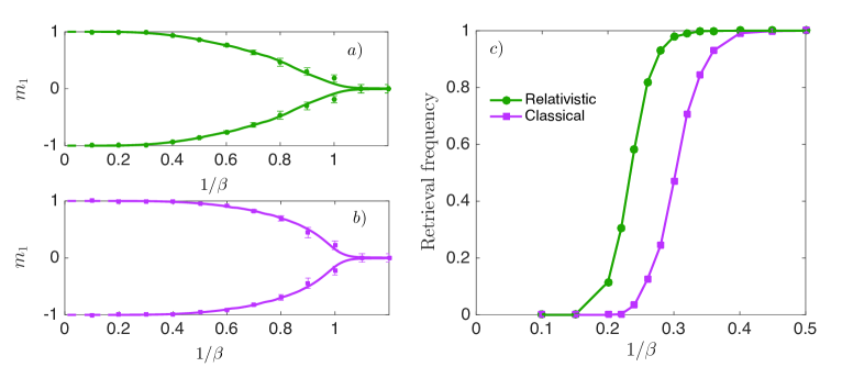
The analysis of the information processing skills of this network has been accomplished elsewhere Albert ; Complexity : we summarize it by Fig. , referring to the original papers for further algorithmic details, while hereafter we deepen the mathematical aspects of its statistical mechanical foundation.
I.3 The statistical mechanical setting
Having defined a suitable Hamiltonian playing as a cost function (see (2) and (4)), the next step in the statistical-mechanics approach requires the introduction of a parameter to account for the noise level in the system (i.e., the inverse temperature in physical jargon) in such a way that for the network evolution is completely random, while in the limit its evolution becomes deterministic (and the Hamiltonian plays as a Lyapounov function Coolen ). Then, we can state the next
Definition 4.
Defined as the average over the patterns, we introduce the partition function and the intensive free energy333Actually, we are committing a small abuse of notation as the “standard” free energy is defined as , but, as from the mathematical side and are (a constant apart) equivalent, we will keep our choice as it makes calculations more transparent, obviously, without affecting the results. as
| (6) | |||||
| (7) |
Definition 5.
Note that defines a probability measure, whose average (Boltzmann average) we indicate with , i.e.
| (8) |
Remark 1.
Note that to highlight when observables are evaluated in the thermodynamic limit, we omit their subscript . For instance, for the free-energy, we write
| (9) |
For the sake of completeness, we recall that for the standard Hopfield model in the infinite volume limit the free energy and the related self-consistency equations for the Mattis overlaps respectively read as Amit ; Coolen ; Viktor
| (10) | |||||
| (11) |
with the abbreviation .
In the following, we will focus solely on the relativistic generalization thus, in order to lighten the notation, we will drop the super- and sub-scripts .
II Existence of the thermodynamic limit of the free energy
In this section we prove the existence of for the relativistic Hopfield model. The underlying idea is to adapt the Guerra-Toninelli scheme, originally developed for a quadratic cost-function, to the Hamiltonian (4) featuring a square root. Following the standard scheme, we consider a system made of neurons and two other, independent, systems made of and neurons such that . Then, we need to prove that the extensive free energy of the former is strictly smaller than the sum of those pertaining to the two subsystems (hence we have its sub-additivity), so that applying the Fekete Lemma fekete we get the result Guerra-LimTerm1 . A way to compare the free energies of these two limiting cases is by interpolation, namely, defining an interpolating free energy whose extrema reproduce the free energies in the two cases of interest and then showing that it derivative -w.r.t. the interpolating parameter- has semi-definite sign. Here the main adaptation will consist in a proof by reduction to absurd assuming the free energy to be super-additive (see Appendix A for the definitions of sub- super-additive successions and functions, and for the main statement of Fekete Lemma).
For the sake of simplicity (and without loss of generality) we fix just in this Section.
Let us consider, beyond the Mattis overlaps related to the patterns of the original -neuron’s model, also two further Mattis overlaps related to the two aforementioned smaller systems made of, respectively, and neurons. We can write
and notice that
once introduced the relative densities as
Definition 6.
Let us introduce an interpolating parameter that we use to define an interpolating free energy as follows
| (12) |
It is crucial to observe that in the two limits of and we recover, respectively,
| (13) |
while
| (14) | |||||
Therefore, by varying , we interpolate between the original system and the sum of the two smaller subsystems, properly weighted by their relative densities. By the Fundamental Theorem of Calculus we can write
| (15) |
and, since the integral operator is monotonous (and therefore it must respect inequalities), it will be sufficient to prove that the derivative of the interpolating free energy w.r.t. , i.e., , has a negative semi-definite sign.
Denoting with the interpolating partition function coupled to the interpolating free energy (12) we can write
| (16) | |||||
where we called
Remark 2.
Now we must prove that the expression averaged in the r.h.s. of eq. (17) is less or equal to zero, as stated by the next
Proposition 1.
The -derivative of the interpolating free energy (12) is semi-definite negative, namely
| (18) |
Proof.
We first observe that, as , the parameters effectively involved in eq. (17) are solely , and , that from now on we will call simply , in such a way that . Then, we can write the l.h.s. of eq. (18) as . Let us now suppose, by contradiction, that
With some algebra we obtain
and, as , we have whence
The r.h.s. term of the above expression is certainly non negative (as ): even in the worst scenario where and have opposite signs, their product will never be smaller than hence, by quadrature the inequality remains unchanged. We are then allowed to write
by which we get
that is obviously wrong. ∎
Remark 3.
We also highlight that the function is convex, namely, for
If we identify
as , then
Theorem 1.
The infinite volume limit of the intensive free energy defined by the relativistic Hopfield cost function (4) exists and it equals its infimum, that is
Proof.
The proof is a straightforward consequence of Proposition coupled to the Fekete Lemma. ∎
III Expression of the thermodynamic limit of the free energy
In this Section we give an explicit expression for the infinite volume limit of the free energy related to the relativistic Hopfield cost-function (4) in terms of the Mattis overlaps. Again, we use a suitable Guerra’s interpolation scheme, in such a way that one extremum of the interpolation recovers the original model to be solved and the other recovers a case whose solution is straightforward. In particular, as we know that all the mean-field models (even the generalized ones) have a product space structure, namely their probability distribution in the thermodynamic limit factorizes (i.e., ), we can use this information to construct the “easy” extremum of the interpolation. In other words,
Definition 7.
Being the scalar an interpolating parameter, we define a novel interpolating free energy as
| (20) |
where , , are fields that are functions of the neurons and of the patterns.
It is worth stressing that each neuron experiences the simultaneous action of fields linearly combined, unlike the interpolating structure working in the ferromagnetic case where each spin just experiences the action of one single field Barra0 . The particular choice of the fields will be discussed later.
Remark 4.
Given a smooth function of the neurons and of the patterns, we observe that the interpolating free-energy (20) implicitly defines the extended averages as
| (21) |
We now must identify the extrema of : at we get the original model we aim to solve, while at we get a system with one-body terms. The latter can be handled easily and its contribution to the free energy reads out as
| (22) |
To obtain the free energy of the model , we use again the Fundamental Theorem of Calculus and write
| (23) |
where, as usual, is the -derivative of the interpolating free energy. The latter reads as
| (24) |
In general, its evaluation is an hard task, yet in the thermodynamic limit (where we are focusing), calling the limiting value of the -th Mattis overlap (i.e., ), by requiring -almost-surely that
| (25) | |||
| (26) |
namely the self-averaging of the order parameters and of the energy of the model Barra0 ; Barra-Bipartiti ; Guerra-SumRules , as we obtain
Comparing the above equation with the r.h.s. of (24) and choosing , we can write
Merging the last result with the Cauchy condition (22) we can finally state the next
Theorem 2.
Remark 5.
We can now move on to study the critical behavior of the system. To this task it will be convenient to introduce the following
Definition 8.
Taking, without loss of generality, as the candidate pattern to be retrieved, we introduce its centered and rescaled Mattis overlap as
| (29) |
where, as usual, while is its thermodynamic limit, namely .
Notice that scales as the variance of times the system size . In this way, we can investigate the critical behaviour of the system by studying as a function of the noise : we look for those values where the fluctuations of the order parameters diverge as this is a signature of criticality.
In order to get an explicit expression for , we exploit again the interpolation scheme (20) and we write as
| (30) |
where the generalized average was defined in (21).
Note that our calculation start at where the system is decoupled: it is thus both natural and convenient to approach the critical line from the high noise region as in this region it is possible to use standard central-limit-theorem-like arguments to assume the probability distribution of the to be a Gaussian444This assumption crucially allows us to use the Wick Theorem, namely, given a Gaussian variable we can write .: the Cauchy condition (that is the standard high-temperature value) can be easily shown to be as as in the ergodic region trivially ).
We must now face the -derivative: to this task it is useful to state the next
Proposition 2.
Retain and let be a smooth function of the Mattis overlaps, then, above and close to the critical point (namely where the Mattis overlaps are zero or infinitesimal) the following streaming equation holds:
| (31) |
Proof.
The proof uses the fact that we are inspecting the critical behavior (hence we assume the Mattis overlap to move from zero continuously when reached a critical noise level) and works by direct brute force:
| (32) |
Expanding and in the above equation and adding and subtracting twice we have the result. ∎
The above Proposition is the key to state the last
Theorem 3.
The centered and rescaled fluctuations of the Mattis overlap (quantifying the retrieval of pattern ) behaves as
| (33) |
thus the high-noise (i.e. ergodic to keep the physical jargon) region is limited to .
In the low-noise (i.e. broken-symmetry) region the Mattis overlap may assume non-null values (see Fig. ).
IV Conclusions and outlooks
In the last decade Artificial Intelligence has permeated our everyday lives and, as a natural consequence, the quest for novel and stronger tools to handle with it has become a urgent priority in different fields of Science DL1 . In particular, within the statistical mechanics route, heuristic and rigorous results appeared steadily in the Theoretical and Mathematical Physics Communities in the last years, typically with heuristic approaches first (as in the case of the standard Hopfield model whose analysis was pioneered by Amit, Gutfreund and Sompolinsky by replica-trick techniques Amit and later confirmed by more rigorous techniques, see e.g., Agliari-Barattolo ; Bovier1 ; Tala1 ).
Along these lines, in this paper, relying on Guerra’s interpolation schemes Guerra-LimTerm1 ; Guerra-SumRules , we have rigorously analyzed the statistical mechanical picture of a new associative neural network, that is, the relativistic Hopfield model recently introduced in Albert . More precisely, by an adaptation of the classical Guerra-Toninelli argument, we have proved that the infinite volume limit of the free energy exists and it is well defined for this model; we also gave its explicit expression in terms of the Mattis overlaps, namely the natural order parameters of the theory, that perfectly matches the results of Albert . Once extremized the free energy over the Mattis overlaps, the self-consistent equations for the order parameters have also been obtained and, with them, a picture of the critical phase transition that the model undergoes when the noise level crosses the critical value . To obtain the explicit expression for the free energy we required the self-averaging (in the infinite volume limit) of the overlaps: this assumption has been confirmed immediately after, by inspecting their (centered and rescaled) fluctuations. The divergence of these fluctuations is found to happen at : this result highlights a critical behavior similar to the one known for the standard Hopfield model in the low-storage regime, despite the presence of many-body contributions.
From a physical viewpoint, this may, at a first glance, sound weird -as -spin systems are known to exhibit discontinuous phase transitions (see e.g., BarraPspin )- however an intuitive explanation for this is that, keeping the r.h.s. of eq. (5) in mind, the pairwise-interaction provides the main driving force toward a broken phase, but the next one, i.e., the fourth-order in (which is anyway small if compared to the previous order as the series (5) obviously converges) appears with the opposite sign thus it drives the system toward a non-magnetized state . Hence we have to wait the even smaller contribution, i.e., sixth-order in , to have another strengthening toward a magnetized state, but this is actually negligible.
From a mathematical viewpoint, instead, the request (25) of the self-averaging of the order parameters gives also a hint that, for the high storage analysis, different approaches would be necessary. This can be understood with a scaling argument by observing that the request (25) breaks down if as the term inside the parenthesis scales as .
Finally, it is worth pointing out that the outlined mathematical scaffold stays robust against pattern’s dilution, namely for multitasking networks Agliari-PRL1 , whose relativistic extension we plan to report soon.
Acknowledgments
A.B. and M.N. acknowledge Salento University.
E.A. and A.B. are grateful to GNFM-INdAM (Progetto Giovani 2018) for financial support.
E.A. acknowledges the grant Progetto Ateneo (RG11715C7CC31E3D) from Sapienza University of Rome.
A.B. also acknowledges MIUR (through basic funding to the Italian research), INFN and the grant Rete Match: Progetto Pythagoras (CUP:J48C17000250006) for financial support.
Appendix A: sub/super-additivity and Fekete Lemma
Definition 9 (sub-additive, super-additive functions).
A function is termed sub-additive (resp. super-additive) if
(resp.
In the same way we can define the concept of sub-additive succession in the following way:
Definition 10 (sub-additive, super-additive successions).
A succession is termed sub-additive (resp. super-additive) if,
(risp.
Lemma 1.
Let be a sub-additive succession, then the follwing holds
Proof.
A sketched proof is immediate by using the Induction Principle over . Indeed, let be a sub-additive succession. If then
Now let us pose and assume the thesis still hold for any natural up to and let us prove it for as well. To be true at it must be that
| (36) |
and thus that
| (37) |
Note that, thanks to the sub-additivity property of the succession, we can write
| (38) |
Merging inequalities (37) and (38) the thesis follows trivially. ∎
Proposition 3 (Lemma di Fekete).
For any sub-additive succession
Similar conclusions can be drawn for super-additive successions as well and in this case case we have that
References
- (1) E. Agliari, et al., Multitasking associative networks, Phys. Rev. Lett. 109, 268101, (2012).
- (2) E. Agliari, A. Barra, A. De Antoni, A. Galluzzi, Parallel retrieval of correlated patterns: From Hopfield networks to Boltzmann machines, Neur. Net. 38, 52, (2013).
- (3) E. Agliari, et al., Retrieval capabilities of hierarchical networks: From Dyson to Hopfield, Phys. Rev. Lett. 114, 028103, (2015).
- (4) E. Agliari, et al., Neural Networks retrieving binary patterns in a sea of real ones, J. Stat. Phys. 168, 1085, (2017).
- (5) E. Agliari, D. Migliozzi, D. Tantari, Non-convex Multi-species Hopfield Models, J. Stat. Phys. 172, 1247, (2018).
- (6) E. Agliari, et al., Complex Reaction Kinetics in Chemistry: A Unified Picture Suggested by Mechanics in Physics, Complexity 2018, 7423297 (2018).
- (7) D.J. Amit, Modeling brain functions, Cambridge Univ. Press (1989).
- (8) A. Barra, The mean field Ising model trough interpolating techniques, J. Stat. Phys. 132(5):787, (2008).
- (9) A. Barra, Notes on ferromagnetic P-spin and REM, Math. Meth. in Appl. Sci. 32:783, (2008).
- (10) A. Barra, M. Beccaria, A. Fachechi,A new mechanical approach to handle generalized Hopfield neural networks, Neural Networks (2018).
- (11) A. Barra, G. Genovese, F. Guerra, Equilibrium statistical mechanics of bipartite spin systems, J. Phys. A (Math. Theor.) 44.24:245002, (2011).
- (12) A. Barra, G. Genovese, F. Guerra, The replica symmetric approximation of the analogical neural network, J. Stat. Phys. 140.4:784, (2010).
- (13) A. Barra, F. Guerra, G. Genovese, D.Tantari, How glassy are neural networks?, JSTAT P07009, (2012).
- (14) A. Bovier, V. Gayrard, Hopfield models as generalized random mean field models, Mathematical aspects of spin glasses and neural networks, Birkhauser Press, Boston, (1998).
- (15) A. Bovier, V. Gayrard, P. Picco, Gibbs states of the Hopfield model in the regime of perfect memory, Prob. Theor. Rel. Fiel. 100(3):329, (1994).
- (16) A.C.C. Coolen, R. Kuhn, P. Sollich, Theory of neural information processing systems, Oxford Press (2005).
- (17) V. Dotsenko, An introduction to the theory of spin glasses and neural networks, World Scientific, (1995).
- (18) A. Fachechi, E. Agliari, A. Barra, Dreaming neural networks: forgetting spurious memories and reinforcing pure ones, submitted to Neur. Net.
- (19) I. Goodfellow, Y. Bengio, A. Courville, Deep Learning, M.I.T. press (2017).
- (20) F. Guerra, Sum rules for the free energy in the mean field spin glass model, Fields Inst. Comm. 30:161, (2001).
- (21) F. Guerra, F.L. Toninelli, The thermodynamic limit in mean field spin glass models, Comm. Math. Phys. 230(1):71-79, (2002).
- (22) F. Guerra, F.L. Toninelli, The infinite volume limit in generalized mean field disordered models, arXiv preprint cond-mat/0208579, (2002).
- (23) J.J. Hopfield, Neural networks and physical systems with emergent collective computational abilities, Proceedings of the national academy of sciences 79.8 (1982): 2554-2558.
- (24) J.J. Hopfield, D.I. Feinstein, R.G. Palmer, Unlearning has a stabilizing effect in collective memories, Nature Lett. 304, 280158, (1983).
- (25) J.A. Horas, P.M. Pasinetti, On the unlearning procedure yielding a high-performance associative memory neural network, J. Phys. A 31, L463-L471, (1998).
- (26) D. Krotov, J.J. Hopfield, Dense associative memory is robust to adversarial inputs, arXiv:1701.00939, (2017).
- (27) Y. Le Cun, Y. Bengio, G. Hinton, Deep learning, Nature 521:436-444, (2015).
- (28) K. Nokura, Spin glass states of the anti-Hopfield model, J. Phys. A 31, 7447, (1998).
- (29) K. Nokura, Paramagnetic unlearning in neural network models, Phys. Rev. E 54(5):5571, (1996).
- (30) K-S. Oh, J. Keechul, GPU implementation of neural networks, Pattern Recognition 37.6:1311, (2004).
- (31) D. Ruelle, Statistical mechanics: Rigorous results, World Scientific, (1999).
- (32) M. Talagrand, Rigorous results for the Hopfield model with many patterns, Prob. Theor. Rel. Fiel. 110(2):177, (1998).
- (33) M. Talagrand, Exponential inequalities and convergence of moments in the replica-symmetric regime of the Hopfield model, Ann. of Prob. 1393, (2000).
- (34) J. Tubiana, R. Monasson, Emergence of compositional representations in restricted Boltzmann machines, Phys. Rev. Lett. 118(13), 138301 (2017).
- (35) S. Wimbauer, J. Leo van Hemmen, Hebbian unlearning, Analysis of Dynamical and Cognitive Systems, Springer, Berlin, 1995.