BDDC preconditioners for a space-time finite element discretization of parabolic problems

Abstract

This paper deals with balanced domain decomposition by constraints (BDDC) method for solving large-scale linear systems of algebraic equations arising from the space-time finite element discretization of parabolic initial-boundary value problems. The time is considered as just another spatial coordinate, and the finite elements are continuous and piecewise linear on unstructured simplicial space-time meshes. We consider BDDC preconditioned GMRES methods for solving the space-time finite element Schur complement equations on the interface. Numerical studies demonstrate robustness of the preconditioners to some extent.

1 Introduction

Continuous space-time finite element methods for parabolic problems have been recently studied, e.g., in REB17 ; UL16 ; UL18 ; OS15 . The main common features of these methods are very different from those of time-stepping methods. Time is considered to be just another spatial coordinate. The variational formulations are studied in the full space-time cylinder that is then decomposed into arbitrary admissible simplex elements. In this work, we follow the space-time finite element discretization scheme proposed in UL18 for a model initial-boundary value problem, using continuous and piecewise linear finite elements in space and time simultaneously.

It is a challenge task to efficiently solve the large-scale linear system of algebraic equations arising from the space-time finite element discretization of parabolic problems. In this work, as a preliminary study, we use the balanced domain decomposition by constraints (BDDC CD03 ; JM03 ; JM05 ) preconditioned GMRES method to solve this system efficiently. We mention that robust preconditioning for space-time isogeometric analysis schemes for parabolic evolution problems has been reported in CH1802 ; CH18 .

The remainder of the paper is organized as follows: Sect. 2 deals with the space-time finite element discretization for a parabolic model problem. In Sect. 3, we discuss BDDC preconditioners that are used to solve the linear system of algebraic equations. Numerical results are shown and discussed in Sect. 4. Finally, some conclusions are drawn in Sect. 5.

2 The space-time finite element discretization

The following parabolic initial-boundary value problem is considered as our model problem: Find $u:\overline{Q}\rightarrow{\mathbb{R}}$ such that

$$\partial_{t}u-\Delta_{x}u=f\textup{ in }Q,\quad u=0\textup{ on }\Sigma,\;u=u_{0}\textup{ on }\Sigma_{0},$$ (1)

where $Q:=\Omega\times(0,T)$, $\Omega\subset{\mathbb{R}}^{2}$ is a sufficiently smooth and bounded computational domain, $\Sigma:=\partial\Omega\times(0,T)$, $\Sigma_{0}:=\Omega\times\{0\}$, $\Sigma_{T}:=\Omega\times\{T\}$.

Let us now introduce the following Sobolev spaces:

$$H_{0}^{1,0}(Q) =\{u\in L_{2}(Q):\nabla_{x}u\in[L_{2}(Q)]^{2},u=0\textup{ on }\Sigma\},$$

$$H_{0,\bar{0}}^{1,1}(Q) =\{u\in L_{2}(Q):\nabla_{x}u\in[L_{2}(Q)]^{2},\partial_{t}u\in L_{2}(Q)\textup{ and }u|_{\Sigma\cup\Sigma_{T}}=0\},$$

$$H_{0,\underline{0}}^{1,1}(Q) =\{u\in L_{2}(Q):\nabla_{x}u\in[L_{2}(Q)]^{2},\partial_{t}u\in L_{2}(Q)\textup{ and }u|_{\Sigma\cup\Sigma_{0}}=0\}.$$

Using the classical approach OAL85 ; OAL68 , the variational formulation for the parabolic model problem (1) reads as follows: Find $u\in H_{0}^{1,0}(Q)$ such that

$$a(u,v)=l(v),\quad\forall v\in H_{0,\bar{0}}^{1,1}(Q),$$ (2)

where

$$a(u,v) =-\int_{Q}u(x,t)\partial_{t}v(x,t)dxdt+\int_{Q}\nabla_{x}u(x,t)\cdot\nabla_{x}u(x,t)dxdt,$$

$$l(v) =\int_{Q}f(x,t)v(x,t)dxdt+\int_{\Omega}u_{0}(x)v(x,0)dx.$$

Remark 1 (Parabolic solvability and regularity OAL85 ; OAL68 )

If $f\in L_{2,1}(Q):=\{v:\int_{0}^{T}\|v(\cdot,t)\|_{L_{2}(\Omega)}dt<\infty\}$ and $u_{0}\in L_{2}(\Omega)$, then there exists a unique generalized solution $u\in H_{0}^{1,0}(Q)\cap V_{2}^{1,0}(Q)$ of (2), where $V_{2}^{1,0}(Q):=\{u\in H^{1,0}(Q):|u|_{Q}<\infty\textup{ and }\displaystyle\lim_{\Delta t\rightarrow 0}\|u(\cdot,t+\Delta t)-u(\cdot,t)\|_{L_{2}(\Omega)}=0,\textup{ uniformly on }[0,T]\}$, and $|u|_{Q}:=\displaystyle\max_{0\leq\tau\leq t}\|u(\cdot,\tau)\|_{L_{2}(\Omega)}+\|\nabla_{x}u\|_{L_{2}(\Omega\times(0,t))}$. If $f\in L_{2}(Q)$ and $u_{0}\in H_{0}^{1}(\Omega)$, then the generalized solution $u$ belongs to $H_{0}^{\Delta,1}(Q):=\{v\in H_{0}^{1,1}(Q):\Delta_{x}u\in L_{2}(Q)\}$ and continuously depends on $t$ in the norm of the space $H_{0}^{1}(\Omega)$.

To derive the space-time finite element scheme, we mainly follow the approach proposed in UL18 . Let $V_{h}=\textup{span}\{\varphi_{i}\}$ be the span of continuous and piecewise linear basis functions $\varphi_{i}$ on shape regular finite elements of an admissible triangulation ${\mathcal{T}}_{h}$. Then we define $V_{0h}=V_{h}\cap H_{0,\underline{0}}^{1,1}(Q)=\{v_{h}\in V_{h}:v_{h}|_{\Sigma\cup\Sigma_{0}}=0\}$. For convenience, we consider homogeneous initial conditions, i.e., $u_{0}=0$ on $\Omega$. Multiplying the PDE $\partial_{t}u-\Delta_{x}u=f$ on $K\in{\mathcal{T}}_{h}$ by an element-wise time-upwind test function $v_{h}+\theta_{K}h_{K}\partial_{t}v_{h}$, $v_{h}\in V_{0h}$, we get

$$\int_{K}(\partial_{t}uv_{h}+\theta_{K}h_{K}\partial_{t}u\partial_{t}v_{h}-\Delta_{x}u(v_{h}+\theta_{K}h_{K}\partial_{t}v_{h}))dxdt=$$

$$\int_{K}f(v_{h}+\theta_{K}h_{K}\partial v_{h})dxdt.$$

Integration by parts (the first part) with respect to the space and summation lead to

$$\sum_{K\in{\mathcal{T}}_{h}}\int_{K}(\partial_{t}uv_{h}+\theta_{K}h_{K}\partial_{t}u\partial_{t}v_{h}+\nabla_{x}u\cdot\nabla_{x}v_{h}-\theta_{K}h_{K}\Delta_{x}u\partial_{t}v_{h})dxdt$$

$$-\sum_{K\in{\mathcal{T}}_{h}}\int_{\partial K}n_{x}\cdot\nabla_{x}uv_{h}ds=\sum_{K\in{\mathcal{T}}_{h}}\int_{K}f(v_{h}+\theta_{K}h_{K}\partial_{t}v_{h})dxdt.$$

Since $n_{x}\cdot\nabla_{x}u$ is continuous on inner boundary of $K$, $n_{x}=0$ on $\Sigma_{0}\cup\Sigma_{T}$, and $v_{h}=0$ on $\Sigma$, the term $-\sum_{K\in{\mathcal{T}}_{h}}\int_{\partial K}n_{x}\cdot\nabla_{x}uv_{h}ds$ vanishes.

If the solution $u$ of (2) belongs to $H_{0,\underline{0}}^{\Delta,1}({\mathcal{T}}_{h}):=\{v\in H_{0,\underline{0}}^{1,1}(Q):\Delta_{x}v|_{K}\in L_{2}(K),\forall K\in{\mathcal{T}}_{h}\}$, cf. Remark 1, then the consistency identity

$$a_{h}(u,v_{h})=l_{h}(v_{h}),\quad v_{h}\in V_{0h},$$ (3)

holds, where

$$a_{h}(u,v_{h}) :=\displaystyle\sum_{K\in{\mathcal{T}}_{h}}\int_{K}(\partial_{t}uv_{h}+\theta_{K}h_{K}\partial_{t}u\partial_{t}v_{h}+\nabla_{x}u\cdot\nabla_{x}v_{h}-\theta_{K}h_{K}\Delta_{x}u\partial_{t}v_{h})dxdt,$$

$$l_{h}(v_{h}) :=\displaystyle\sum_{K\in{\mathcal{T}}_{h}}\int_{K}f(v_{h}+\theta_{K}h_{K}\partial_{t}v_{h})dxdt.$$

With the restriction of the solution to the finite-dimensional subspace $V_{0h}$, the space-time finite element scheme reads as follows: Find $u_{h}\in V_{0h}$ such that

$$a_{h}(u_{h},v_{h})=l_{h}(v_{h}),\quad v_{h}\in V_{0h}.$$ (4)

Thus, we have the Galerkin orthogonality: $a_{h}(u-u_{h},v_{h})=0$, $\forall v_{h}\in V_{0h}$.

Remark 2

Since we use continuous and piecewise linear trial functions, the integrand $-\theta_{K}h_{K}\Delta_{x}u_{h}\partial_{t}v_{h}$ vanishes element-wise, which simplifies the implementation.

Remark 3

On fully unstructured meshes, $\theta_{k}=O(h_{k})$ UL18 ; on uniform meshes, $\theta_{k}=\theta=O(1)$ UL16 . In this work, we have used $\theta=0.5$ and $\theta=2.5$ on uniform meshes for testing robustness of the BDDC preconditioners.

It was shown in UL18 that the bilinear form $a_{h}(\cdot,\cdot)$ is $V_{0h}$-coercive: $a_{h}(v_{h},v_{h})\geq\mu_{c}\|v_{h}\|_{h}^{2}$, $\forall v_{h}\in V_{0h}$ with respect to the norm $\|v_{h}\|_{h}^{2}=\sum_{K\in{\mathcal{T}}_{h}}(\|\nabla_{x}v_{h}\|_{L_{2}(K)}^{2}+\theta_{K}h_{K}\|\partial_{t}v_{h}\|_{L_{2}(K)}^{2})+\frac{1}{2}\|v_{h}\|^{2}_{L_{2}(\Sigma_{T})}$. Furthermore, the bilinear form is bounded on $V_{0h,*}\times V_{0h}$: $|a_{h}(u,v_{h})|\leq\mu_{b}\|u\|_{0h,*}\|v_{h}\|_{h}$, $\forall u\in V_{0h,*}$, $\forall v_{h}\in V_{0h}$, where $V_{0h,*}=H_{0,\underline{0}}^{\Delta,1}({\mathcal{T}}_{h})+V_{0h}$ equipped with the norm $\|v\|_{0h,*}^{2}=\|v\|_{h}^{2}+\sum_{K\in{\mathcal{T}}_{h}}(\theta_{K}h_{K})^{-1}\|v\|_{L_{2}(K)}^{2}$ $+\sum_{K\in{\mathcal{T}}_{h}}\theta_{k}h_{k}\|\Delta_{x}v\|_{L_{2}(K)}^{2}$. Let $l$ and $k$ be positive reals such that $l\geq k>3/2$. We now define the broken Sobolev space $H^{s}({\mathcal{T}}_{h}):=\{v\in L_{2}(Q):v|_{K}\in H^{s}(K)$ $\forall K\in{\mathcal{T}}_{h}\}$ equipped with the broken Sobolev semi-norm $|v|^{2}_{H^{s}({\mathcal{T}}_{h})}:=\sum_{K\in{\mathcal{T}}_{h}}|v|_{H^{s}(K)}^{2}$. Using the Lagrangian interpolation operator $\Pi_{h}$ mapping $H_{0,\underline{0}}^{1,1}(Q)\cap H^{k}(Q)$ to $V_{0h}$, we obtain $\|u-u_{h}\|_{h}\leq\|u-\Pi_{h}u\|_{h}+\|\Pi_{h}u-u_{h}\|_{h}$. The term $\|u-\Pi_{h}u\|_{h}$ can be bounded by means of the interpolation error estimate, and the term $\|\Pi_{h}u-u_{h}\|_{h}$ by using ellipticity, Galerkin orthogonality and boundedness of the bilinear form. The discretization error estimate $\|u-u_{h}\|_{h}\leq C(\sum_{K\in{\mathcal{T}}_{h}}h_{K}^{2(l-1)}|u|^{2}_{H^{l}(K)})^{1/2}$ holds for the solution $u$ provided that $u$ belongs to $H_{0,\underline{0}}^{1,1}(Q)\cap H^{k}(Q)\cap H^{l}({\mathcal{T}}_{h})$, and the finite element solution $u_{h}\in V_{0h}$, where $C>0$, independent of mesh size; see UL18 .

3 Two-level BDDC preconditioners

After the space-time finite element discretization of the model problem (1), the linear system of algebraic equations reads as follows:

$$Kx=f,$$ (5)

with $K:=\begin{bmatrix}K_{II}&K_{I\Gamma}\\ K_{\Gamma I}&K_{\Gamma\Gamma}\\ \end{bmatrix}$, $x:=\begin{bmatrix}x_{I}\\ x_{\Gamma}\\ \end{bmatrix}$, $f:=\begin{bmatrix}f_{I}\\ f_{\Gamma}\\ \end{bmatrix}$, $K_{II}=\text{diag}\left[K_{II}^{1},...,K_{II}^{N}\right]$, where $N$ denotes the number of polyhedral subdomains $\Omega_{i}$ from a non-overlapping domain decomposition of $\Omega$. In system (5), we have decomposed the degrees of freedom into the ones associated with the internal ($I$) and interface ($\Gamma$) nodes, respectively. We aim to solve the Schur-complement system living on the interface:

$$Sx_{\Gamma} =g_{\Gamma},$$ (6)

with $S:=K_{\Gamma\Gamma}-K_{\Gamma I}K_{II}^{-1}K_{I\Gamma}$ and $g:=f_{\Gamma}-K_{\Gamma I}K_{II}^{-1}f_{I}$.

Following JM05 (see also details in LJ06 ), Dohrmann’s (two-level) BDDC preconditioners $P_{BDDC}$ for the interface Schur complement equation (6), originally proposed for symmetric and positive definite systems in CD03 ; JM03 , can be written in the form

$$P_{BDDC}^{-1}=R_{D,\Gamma}^{T}(T_{sub}+T_{0})R_{D,\Gamma},$$ (7)

where the scaled operator $R_{D,\Gamma}$ is the direct sum of restriction operators $R_{D,\Gamma}^{i}$ mapping the global interface vector to its component on local interface $\Gamma_{i}:=\partial\Omega_{i}\cap\Gamma$, with a proper scaling factor.

Here the coarse level correction operator $T_{0}$ is constructed as

$$T_{0}=\Phi(\Phi^{T}S\Phi)^{-1}\Phi^{T}$$ (8)

with the coarse level basis function matrix $\Phi=\left[(\Phi^{1})^{T},\cdots,(\Phi^{N})^{T}\right]^{T}$, where the basis function matrix $\Phi^{i}$ on each subdomain interface is obtained by solving the following augmented system:

$$\begin{bmatrix}S^{i}&\left(C^{i}\right)^{T}\\ C^{i}&0\end{bmatrix}\begin{bmatrix}\Phi^{i}\\ \Lambda^{i}\\ \end{bmatrix}=\begin{bmatrix}0\\ R_{\Pi}^{i}\\ \end{bmatrix}.$$ (9)

with the given primal constraints $C^{i}$ of the subdomain $\Omega_{i}$ and the vector of Lagrange multipliers on each column of $\Lambda^{i}$. The number of columns of each $\Phi^{i}$ equals to the number of global coarse level degrees of freedom, typically living on the subdomain corners, and/or interface edges, and/or faces. Here the restriction operator $R_{\Pi}^{i}$ maps the global interface vector in the continuous primal variable space on the coarse level to its component on $\Gamma_{i}$.

The subdomain correction operator $T_{sub}$ is defined as

$$T_{sub}=\displaystyle\sum_{i=1}^{N}\left[(R_{\Gamma}^{i})^{T}\quad 0\right]\begin{bmatrix}&S^{i}&\left(C^{i}\right)^{T}\\ &C^{i}&0\end{bmatrix}^{-1}\begin{bmatrix}&R_{\Gamma}^{i}\\ &0\end{bmatrix},$$ (10)

with vanishing primal variables on all the coarse levels. Here the restriction operator $R_{\Gamma}^{i}$ maps global interface vectors to their components on $\Gamma_{i}$.

4 Numerical experiments

We use $u(x,y,t)=\sin(\pi x)\sin(\pi y)\sin(\pi t)$ as exact solution of (1) in $Q=(0,1)^{3}$; see the left plot in Fig. 1. We perform uniform mesh refinements of $Q$ using tetrahedral elements. By using Metis GK98 , the domain is decomposed into $N=2^{k}$, $k=3,4,...,9$, non-overlapping subdomains $\Omega_{i}$ with their own tetrahedral elements; see the right plot in Fig. 1. The total number of degrees of freedom is $(2^{k}+1)^{3}$, $k=4,5,6,7$. We run BDDC preconditioned GMRES iterations until the relative residual error reaches $10^{-9}$. Three variants of BDDC preconditioners are used with corner ($C$), corner/edge ($CE$), and corner/edge/face ($CEF$) constraints, respectively. The number of BDDC preconditioned GMRES iterations and the computational time measured in seconds [s] are given in Table 1, with respect to the number of subdomains (row-wise) and number of degrees of freedom (column-wise). Since the system is unsymmetric but positive definite, the BDDC preconditioners do not show the same typical robustness and efficiency behavior when applied to the symmetric and positive definite system AT04 . Nevertheless, we still observe certain scalability with respect to the number subdomains (up to $128$), in particular, with corner/edge and corner/edge/face constraints. For $\theta=2.5$, we see improvement of BDDC preconditioners with respect to the number of GMRES iterations and computational time; see Table 2. Further, we observe improved scalability with respect to the number of subdomains as well as number of degrees of freedom.

[scale=.15]HeatOn512CPUs.png 

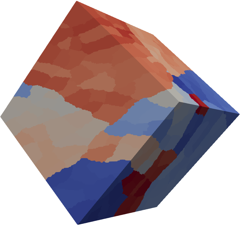
Figure 1: Solution (left), space-time domain decomposition (right) with $129^{3}$ degrees of freedom and $512$ subdomains.

Table 1: $\theta=0.5$. BDDC performance using different coarse level constraints ($C$/$CE$/$CEF$).

No preconditioner
	$8$	$16$	$32$	$64$	$128$	$256$	$512$
$17^{3}$	$52$	$59$	$63$	$71$	$76$	$>500$	$>500$
	($0.04s$)	($0.03s$)	($0.03s$)	($0.04s$)	($0.05s$)	$-$	$-$
$33^{3}$	$86$	$100$	$113$	$126$	$144$	$>500$	$>500$
	($0.76s$)	($0.41s$)	($0.22s$)	($0.18s$)	($0.33s$)	$-$	$-$
$65^{3}$	$149$	$176$	$206$	$225$	$260$	$294$	$>500$
	($35.32s$)	($13.55s$)	($6.05s$)	($2.88s$)	($2.02s$)	($5.78s$)	$-$
$129^{3}$	OoM	OoM	$346$	$399$	$467$	$>500$	$>500$
	($-$)	($-$)	($213.23s$)	($89.23s$)	($41.51s$)	($-$)	($-$)
$C$ (corner) preconditioner
$17^{3}$	$24$	$31$	$30$	$38$	$44$	$56$	$114$
	($0.03s$)	($0.02s$)	($0.02s$)	($0.03s$)	($0.08s$)	($0.32s$)	($2.7s$)
$33^{3}$	$34$	$40$	$57$	$78$	$75$	$247$	$233$
	($0.65s$)	($0.30s$)	($0.21s$)	($0.19s$)	($0.27s$)	($2.11s$)	($8.33s$)
$65^{3}$	$40$	$64$	$92$	$126$	$149$	$166$	$476$
	($22.56s$)	($10.05s$)	($5.26s$)	($2.95s$)	($1.70s$)	($4.95s$)	($19.56s$)
$129^{3}$	OoM	OoM	$173$	$250$	$286$	$>500$	$311$
	($-$)	($-$)	($227.67s$)	($113.38s$)	($47.2s$)	($-$)	($20.40s$)
$CE$ (corner+edge) preconditioner
$17^{3}$	$23$	$25$	$24$	$26$	$29$	$44$	$70$
	($0.03s$)	($0.02s$)	($0.02s$)	($0.03s$)	($0.12s$)	($0.32s$)	($1.52s$)
$33^{3}$	$32$	$32$	$35$	$49$	$40$	$124$	$146$
	($0.63s$)	($0.27s$)	($0.13s$)	($0.15s$)	($0.23s$)	($1.59s$)	($7.19s$)
$65^{3}$	$38$	$56$	$72$	$85$	$87$	$89$	$295$
	($21.93s$)	($9.02s$)	($4.37s$)	($2.10s$)	($1.23s$)	($3.43s$)	($21.59s$)
$129^{3}$	OoM	OoM	$139$	$177$	$196$	$>500$	$218$
	($-$ )	($-$)	($184.57s$)	($82.38s$)	($33.43s$)	($-$)	($23.76s$)
$CEF$ (corner+edge+face) preconditioner
$17^{3}$	$22$	$24$	$23$	$24$	$23$	$39$	$72$
	($0.03s$)	($0.02s$)	($0.02s$)	($0.04s$)	($0.09$)	($0.32s$)	($1.47s$)
$33^{3}$	$33$	$31$	$35$	$46$	$37$	$119$	$134$
	($0.80s$)	($0.33s$)	($0.17s$)	($0.17s$)	($0.32s$)	($2.51s$)	$8.2s$
$65^{3}$	$39$	$55$	$70$	$80$	$81$	$80$	$275$
	($21.56s$)	($11.52s$)	($5.61s$)	($2.50s$)	($2.14s$)	($4.04s$)	($48.58s$)
$129^{3}$	OoM	OoM	$173$	$171$	$185$	$>500$	$206$
	($-$)	($-$)	($226.93s$)	($109.94s$)	($45.05s$)	($-$)	$(33.13s$)

Table 2: $\theta=2.5$. BDDC performance using different coarse level constraints ($C$/$CE$/$CEF$).

No preconditioner
	$8$	$16$	$32$	$64$	$128$	$256$	$512$
$17^{3}$	$46$	$51$	$55$	$61$	$66$	$>500$	$>500$
	($0.02s$)	($0.02s$)	($0.02s$)	($0.03s$)	($0.04s$)	$-$	$-$
$33^{3}$	$72$	$79$	$87$	$99$	$108$	$>500$	$>500$
	($0.64s$)	($0.32s$)	($0.15s$)	($0.12s$)	($0.13s$)	$-$	$-$
$65^{3}$	$116$	$126$	$145$	$163$	$176$	$191$	$>500$
	($27.59s$)	($9.17s$)	($4.07s$)	($1.92s$)	($1.06s$)	($2.02s$)	$-$
$129^{3}$	OoM	OoM	$240$	$271$	$304$	$>500$	$382$
	($-$)	($-$)	($145.64s$)	($58.51s$)	($24.3s$)	($-$)	($12.41s$)
$C$ (corner) preconditioner
$17^{3}$	$23$	$28$	$27$	$32$	$36$	$51$	$110$
	($0.02s$)	($0.02s$)	($0.03s$)	($0.03s$)	($0.07s$)	($0.72s$)	($2.48s$)
$33^{3}$	$30$	$33$	$39$	$50$	$50$	$206$	$182$
	($0.60s$)	($0.26s$)	($0.14s$)	($0.10s$)	($0.09s$)	($3.86s$)	($6.2s$)
$65^{3}$	$35$	$47$	$61$	$64$	$69$	$77$	$287$
	($19.85s$)	($7.42s$)	($3.47s$)	($1.44s$)	($0.68s$)	($1.05s$)	($9.00s$)
$129^{3}$	OoM	OoM	$94$	$104$	$107$	$340$	$112$
	($-$)	($-$)	($124.30s$)	($46.45s$)	($16.90s$)	($33.45s$)	($5.89s$)
$CE$ (corner+edge) preconditioner
$17^{3}$	$21$	$22$	$22$	$25$	$27$	$42$	$80$
	($0.03s$)	($0.02s$)	($0.01s$)	($0.03s$)	($1.78s$)	($0.78s$)	($1.65s$)
$33^{3}$	$27$	$26$	$32$	$38$	$32$	$117$	$132$
	($0.54s$)	($0.23s$)	($0.11s$)	($0.12s$)	($0.15s$)	($2.52s$)	($5.98s$)
$65^{3}$	$33$	$44$	$51$	$54$	$54$	$54$	$235$
	($19.00s$)	($7.27s$)	($2.98s$)	($1.33s$)	($0.75s$)	($1.32s$)	($15.13s$)
$129^{3}$	OoM	OoM	$82$	$83$	$90$	$366$	$94$
	($-$)	($-$)	($109.19s$)	($38.59s$)	($15.21s$)	($37.00s$)	($7.91s$)
$CEF$ (corner+edge+face) preconditioner
$17^{3}$	$21$	$21$	$22$	$22$	$22$	$38$	$74$
	($0.02s$)	($0.01s$)	($0.02s$)	($0.04s$)	($0.13s$)	($0.74s$)	($1.74s$)
$33^{3}$	$27$	$26$	$30$	$35$	$31$	$115$	$123$
	($0.68s$)	($0.28s$)	($0.14s$)	($0.12s$)	($0.25s$)	($3.79s$)	($7.08s$)
$65^{3}$	$34$	$44$	$49$	$52$	$53$	$51$	$226$
	($26.64s$)	($9.29s$)	($3.86s$)	($1.61s$)	($1.11s$)	($1.88s$)	$21.30s$
$129^{3}$	OoM	OoM	$82$	$83$	$88$	$369$	$92$
	($-$)	($-$)	($145.39s$)	($53.10s$)	($23.04s$)	($52.33$)	($13.8s$)

5 Conclusions

In this work, we have applied two-level BDDC preconditioned GMRES methods to the solution of finite element equations arising from the space-time discretization of a parabolic model problem. We have compared the performance of BDDC preconditioners with different coarse level constraints for such an unsymmetric, but positive definite system. The preconditioners show certain scalability provided that $\theta$ is sufficiently large. Future work will concentrate on improvement of coarse-level corrections in order to achieve robustness with respect to different choices of $\theta$.

References

• [1] R. E. Bank, P. S. Vassilevski, and L. T. Zikatanov. Arbitrary dimension convection-diffusion schemes for space-time discretizations. J. Comput. Appl. Math., 310:19–31, 2017.
• [2] C. R. Dohrmann. A preconditioner for substructuring based on constrained energy minimization. SIAM J. Sci. Comput., 25(1):246–258, 2003.
• [3] C. Hofer, U. Langer, and M. Neumüller. Robust preconditioning for space-time isogeometric analysis of parabolic evolution problems. Technical report, 2018. arXiv:1802.09277 [math.NA].
• [4] C. Hoffer, U. Langer, M. Neumüller, and I. Toulopoulos. Time-multipatch discontinuous Galerkin space-time isogeometric analysis of parabolic evolution problems. Electron. Trans. Numer. Anal., 49:126–150, 2018.
• [5] L. Jing and O. B. Widlund. FETI-DP, BDDC, and block Cholesky methods. Int. J. Numer. Meth. Engng., 66(2):250–271, 2006.
• [6] G. Karypis and V. Kumar. A fast and high quality multilevel scheme for partitioning irregular graphs. SIAM Journal on Scientific Computing, 20(1):359–392, 1998.
• [7] O. A. Ladyžhenskaya. The boundary value problems of mathematical physics, volume 49 of Applied Mathematical Sciences. Springer-Verlag, New York, 1985.
• [8] O. A. Ladyžhenskaya, V. A. Solonnikov, and N. N. Uraltseva. Linear and quasilinear equations of parabolic type. AMS, Providence, RI, 1968.
• [9] U. Langer, S. E. Moore, and M. Neumüller. Space-time isogeometric analysis of parabolic evolution problems. Comput. Methods Appl. Mech. Eng., 306:342–363, 2016.
• [10] U. Langer, M. Neumüller, and A. Schafelner. Space-time finite element methods for parabolic evolution problems with variable coefficients. In T. Apel, U. Langer, A. Meyer, and O. Steinbach, editors, Advanced finite element methods with applications - Proceedings of the 30th Chemnitz FEM symposium 2017, pages xx1–y27. Springer, Berlin, Heidelberg, New York, 2019. accepted for publication.
• [11] J. Mandel and C. R. Dohrmann. Convergence of a balancing domain decomposition by constraints and energy minimization. Numer. Linear Algebra Appl., 10(7):639–659, 2003.
• [12] J. Mandel, C. R. Dohrmann, and R. Tezaur. An algebraic theory for primal and dual substructuring methods by constraints. Appl. Numer. Math., 54(2):167–193, 2005.
• [13] O. Steinbach. Space-time finite element methods for parabolic problems. Comput. Methods Appl. Math., 15:551–566, 2015.
• [14] A. Toselli and O. B. Widlund. Domain decomposition methods - Algorithms and theory, volume 34 of Springer Series in Computational Mathematics. Springer, Berlin, Heidelberg, New York, 2004.