a Stanford Institute for Theoretical Physics, Stanford University,
Stanford, CA 94305, USA

b Department of Physics, University of California,
Santa Barbara, CA 93106, USA

xlqi@stanford.edu | alex@physics.ucsb.edu

In many-body chaotic systems, the size of an operator generically grows in Heisenberg evolution, which can be measured by certain out-of-time-ordered four-point functions. However, these only provide a coarse probe of the full underlying operator growth structure. In this article we develop a methodology to derive the full growth structure of fermionic systems, that also naturally introduces the effect of finite temperature. We then apply our methodology to the SYK model, which features all-to-all q𝑞q-body interactions. We derive the full operator growth structure in the large q𝑞q limit at all temperatures. We see that its temperature dependence has a remarkably simple form consistent with the slowing down of scrambling as temperature is decreased. Furthermore, our finite-temperature scrambling results can be modeled by a modified epidemic model, where the thermal state serves as a vaccinated population, thereby slowing the overall rate of infection.

1 Introduction & Summary

In chaotic quantum many-body systems, operators grow in size as time evolves. For example, in spatially local systems one expects that the extent of an operator 𝒪(t)𝒪𝑡\mathcal{O}\left(t\right) grows as

ddtVolume[𝒪(t)]Surface Area[𝒪(t)]proportional-to𝑑𝑑𝑡Volumedelimited-[]𝒪𝑡Surface Areadelimited-[]𝒪𝑡\frac{d}{dt}\textrm{Volume}\left[\mathcal{O}\left(t\right)\right]\propto\textrm{Surface Area}\left[\mathcal{O}\left(t\right)\right] (1.1)

since the new terms generated by taking [H,𝒪(t)]𝐻𝒪𝑡\left[H,\mathcal{O}\left(t\right)\right] will live on the boundary of the domain of 𝒪(t)𝒪𝑡\mathcal{O}\left(t\right) [1, 2, 3, 4]. Consequently, the extent grows linearly with an effective "speed of light" vtsimilar-to-or-equalsabsent𝑣𝑡\simeq vt. Up to exponential error all operators outside the effective light-cone will commute with 𝒪(t)𝒪𝑡\mathcal{O}\left(t\right). This effective speed of light is known as the Lieb-Robinson velocity [1]. This highlights the fact that space can be a derived concept in quantum mechanics, as without the Hamiltonian there may not be a sense in which one piece of the Hilbert space factorization is closer to another.

Now we would like to contrast this behavior with that exhibited by q𝑞q-local systems, where the Hamiltonian couples all the degrees of freedom together in q𝑞q-body interactions. Consequently, there is no notion of spatial locality, and we accordingly refer to such interactions as coupling together “internal” degrees of freedom. Yet, there remains structure in the evolution of operators in these systems, as we often find that the sizes of operators grow exponentially

ddtSize[𝒪(t)]Size[𝒪(t)]proportional-to𝑑𝑑𝑡Sizedelimited-[]𝒪𝑡Sizedelimited-[]𝒪𝑡\frac{d}{dt}\mathrm{Size}\left[\mathcal{O}\left(t\right)\right]\propto\mathrm{Size}\left[\mathcal{O}\left(t\right)\right] (1.2)

where by size we mean the number of simple operators multiplied together in a typical piece of 𝒪(t)𝒪𝑡\mathcal{O}\left(t\right). The intuition behind this growth is that the percentage of the q𝑞q-body interactions utilized in [H,𝒪(t)]𝐻𝒪𝑡\left[H,\mathcal{O}\left(t\right)\right] is proportional to the size of 𝒪(t)𝒪𝑡\mathcal{O}\left(t\right), and almost all the resultant operators obtained from [H,𝒪(t)]𝐻𝒪𝑡\left[H,\mathcal{O}\left(t\right)\right] are bigger than 𝒪(t)𝒪𝑡\mathcal{O}\left(t\right) [5, 6, 7, 8, 9, 10, 11].111Eq. (1.2) actually can be considered as the same formula as in Eq. (1.1) applied to a completely connected graph, so that the area of a region is proportional to its volume [9].

Systems with both spatial locality and a large number of internal degrees of freedom–such as (chaotic) field theories in the large-N𝑁N limit – display both linear spatial growth and exponential internal size growth [12, 13, 14, 15, 16]. The growth of an evolving simple operator W(t)𝑊𝑡W\left(t\right) can be probed using another simple operator V𝑉V, using the (anti-)commutator squared |[W(t),V]|2expectation-valuesuperscript𝑊𝑡𝑉2\expectationvalue*{\left|\left[W\left(t\right),V\right]\right|^{2}} or their corresponding out-of-time-order correlator (OTOC) W(t)VW(t)Vdelimited-⟨⟩superscript𝑊𝑡superscript𝑉𝑊𝑡𝑉\left\langle W^{\dagger}\left(t\right)V^{\dagger}W\left(t\right)V\right\rangle [17, 18, 19, 20, 21, 12, 22, 23, 24, 25].

In order to develop the coarse-grained profile of operator growth, one must compute many OTOCs. The “chaos bound” [26] obeyed by OTOCs suggests that after an initial dissipation time, they de-correlate no faster than exponentially, with a rate λLsubscript𝜆𝐿\lambda_{L} no larger than 2πT2𝜋𝑇2\pi T where T=1/β𝑇1𝛽T=1/\beta is the temperature. This implies that presence of the thermal state ρexp(βH)proportional-to𝜌𝛽𝐻\rho\propto\exp\left(-\beta H\right) slows down the effective growth rate of operators as temperature is decreased.

The Heisenberg evolution of operator 𝒪(t)𝒪𝑡\mathcal{O}\left(t\right) is independent of temperature, so the entire effect of temperature must be contained in the matrix elements of 𝒪𝒪\mathcal{O}. Therefore, the natural finite temperature generalization of operator size has remained an open question (one recent proposal is given in [27]).

In this article, we address this issue by characterizing not only the average size of an operator but its entire size distribution. We then can define the effective size distribution of an operator at finite temperature by how it changes the size of the square root of thermal density operator ρ1/2superscript𝜌12\rho^{1/2} (we explain why this is a natural choice in section (3)).

This definition leads to some nontrivial general results, independent of the details of the specific physical system. In particular, we observe that in generic fermion systems, the effective size of a single fermion operator is “thermally renormalized” to a value δβ=G(β/2)subscript𝛿𝛽𝐺𝛽2\delta_{\beta}=G\left(\beta/2\right) smaller than 111, where G(τ)𝐺𝜏G\left(\tau\right) is the thermal two-point function. The size of the thermal operator ρ1/2superscript𝜌12\rho^{1/2} itself is N2(1δβ)𝑁21subscript𝛿𝛽\frac{N}{2}\left(1-\delta_{\beta}\right), determined by the same renormalization factor δβsubscript𝛿𝛽\delta_{\beta}. To gain a more explicit understanding, we will work in the context of the SYK model [28, 29], a q𝑞q-local Hamiltonian built out of N𝑁N flavors of Majorana fermions, which saturates the chaos bound at low temperatures [30, 20, 29]

The remainder of the article is organized as follows. We begin in section (2) by building up the notion of operator “size”. First, we show that one may expand any operator 𝒪(t)𝒪𝑡\mathcal{O}\left(t\right) in an orthonormal operator basis of the unique products of Majorana flavors. In the doubled theory, the operator basis maps to an orthonormal basis of states in the doubled Hilbert space. We define a “size” operator n𝑛n in the doubled theory counting the average number of flavors in an operator basis state. We are then able to demonstrate that four-point functions measure the average “size” of an operator. Therefore, the de-correlation of a thermal OTOC is exactly equivalent to the growing average size of the operator ψ1(t)ρ1/2subscript𝜓1𝑡superscript𝜌12\psi_{1}\left(t\right)\rho^{1/2}

1Nj=1NTr(ρ1/2ψ1(t)ψjψ1(t)ρ1/2ψj)=12Nn[ψ1(t)ρ1/2]1𝑁superscriptsubscript𝑗1𝑁tracesuperscript𝜌12subscript𝜓1𝑡subscript𝜓𝑗subscript𝜓1𝑡superscript𝜌12subscript𝜓𝑗12𝑁𝑛delimited-[]subscript𝜓1𝑡superscript𝜌12-\frac{1}{N}\sum_{j=1}^{N}\Tr\left(\rho^{1/2}\psi_{1}\left(t\right)\psi_{j}\psi_{1}\left(t\right)\rho^{1/2}\psi_{j}\right)=1-\frac{2}{N}n\left[\psi_{1}\left(t\right)\rho^{1/2}\right] (1.3)

The average size of the operator ψ1(t)ρ1/2subscript𝜓1𝑡superscript𝜌12\psi_{1}\left(t\right)\rho^{1/2} starts at n[ψ1ρ1/2]n[ρ1/2]=N2(1δβ)𝑛delimited-[]subscript𝜓1superscript𝜌12𝑛delimited-[]superscript𝜌12𝑁21subscript𝛿𝛽n\left[\psi_{1}\rho^{1/2}\right]\approx n\left[\rho^{1/2}\right]=\frac{N}{2}\left(1-\delta_{\beta}\right) and then grows sigmoidally in time, eventually saturating (scrambling) at a value of N/2𝑁2N/2.

Up to this point we have been discussing the average size of the operator ψ(t)ρ1/2𝜓𝑡superscript𝜌12\psi\left(t\right)\rho^{1/2}. In fact, the entire size distribution of this operator has physical significance. Hence, in section (3) we construct generating functions for operator size distributions by inserting a weighting factor exp(μn)𝜇𝑛\exp\left(-\mu n\right). First, we study the size distribution of the thermal operator ρ1/2superscript𝜌12\rho^{1/2} by setting up a generating function 𝒵μ[ρ1/2]subscript𝒵𝜇delimited-[]superscript𝜌12\mathcal{Z}_{\mu}\left[\rho^{1/2}\right], which is similar to a grand canonical partition function. Next, we show that the fractional distance to scrambling for the operator ρ1/2superscript𝜌12\rho^{1/2} is always given by δβ1n/n=G(β/2)<1subscript𝛿𝛽1𝑛subscript𝑛𝐺𝛽21\delta_{\beta}\equiv 1-n/n_{*}=G\left(\beta/2\right)<1. Then, we set up the generating function for the size distribution of ψ(t)ρ1/2𝜓𝑡superscript𝜌12\psi\left(t\right)\rho^{1/2}, which we find naturally splits into a product of 𝒵μ[ρ1/2]subscript𝒵𝜇delimited-[]superscript𝜌12\mathcal{Z}_{\mu}\left[\rho^{1/2}\right] and a modified two-point function 𝒢μ(t)subscript𝒢𝜇𝑡\mathcal{G}_{\mu}\left(t\right). We show that the μ𝜇\mu-expansion of 𝒢μ(t)subscript𝒢𝜇𝑡\mathcal{G}_{\mu}\left(t\right) determines the growth distribution induced by multiplying ρ1/2superscript𝜌12\rho^{1/2} by ψ(t)𝜓𝑡\psi\left(t\right), and that 𝒢μ(t)subscript𝒢𝜇𝑡\mathcal{G}_{\mu}\left(t\right) is simply the two-point function for the original theory with a μ𝜇\mu-dependent twisted boundary condition. We conclude the section by noting that on average, the size increase induced by a single fermion is given by the fractional scrambling distance δβsubscript𝛿𝛽\delta_{\beta}, which leads us to propose that δβsubscript𝛿𝛽\delta_{\beta} should be interpreted as a thermally renormalized unit of size.

Everything in sections (2) and (3) applies to general fermionic systems. In sections (4) and (5), we apply this methodology to the large-q𝑞q SYK model. Solving the large-N𝑁N saddle point equation in the large q𝑞q limit with our μ𝜇\mu-dependent twist, we obtain the full operator growth structure. After a dynamical renormalization of coupling constant 𝒥𝒥\mathcal{J} (which after a short amount of time essentially amounts to replacing the coupling with a smaller β𝛽\beta-dependent constant) and a renormalization of size unit from 111 to δβsubscript𝛿𝛽\delta_{\beta}, we observe that the full growth structure has the same functional form as the infinite temperature case. The dynamical renormalization of the coupling is the signature of the slowdown of the effective growth rate as temperature is decreased.

We conclude the section by discussing how to understand this finite temperature slowdown of scrambling in an epidemic model, where the thermal factor effectively vaccinates a large subset of the population, thereby slowing down the overall infection rate. We end the paper by discussing implications and future directions in section (6).

2 Operator Distributions and Two-Sided Wavefunctions

As an operator 𝒪(t)𝒪𝑡\mathcal{O}\left(t\right) evolves in time, it becomes supported along operators of increasing size. This can be inferred from the Heisenberg equation of motion 𝒪˙(t)=i[H,𝒪(t)]˙𝒪𝑡𝑖𝐻𝒪𝑡\dot{\mathcal{O}}\left(t\right)=i\left[H,\mathcal{O}\left(t\right)\right]. Now, in order to properly discuss how much one operator is supported along another, we need an operator inner product. When the Hilbert space is finite-dimensional it is natural to use the Frobenius inner product: 𝒪A|𝒪BTr(𝒪A𝒪B)inner-productsubscript𝒪𝐴subscript𝒪𝐵Trsuperscriptsubscript𝒪𝐴subscript𝒪𝐵\innerproduct*{\mathcal{O}_{A}}{\mathcal{O}_{B}}\equiv\mathrm{Tr}(\mathcal{O}_{A}^{\dagger}\mathcal{O}_{B}). We may then expand operators in an orthonormal operator basis, which amounts to inserting a complete set of operators {ΓI}subscriptΓ𝐼\left\{\Gamma_{I}\right\}

𝒪(t)=IΓITr(ΓI𝒪(t))IcI(t)ΓI𝒪𝑡subscript𝐼subscriptΓ𝐼TrsuperscriptsubscriptΓ𝐼𝒪𝑡subscript𝐼subscript𝑐𝐼𝑡subscriptΓ𝐼\mathcal{O}\left(t\right)=\sum_{I}\Gamma_{I}\mathrm{Tr}\left(\Gamma_{I}^{\dagger}\mathcal{O}\left(t\right)\right)\equiv\sum_{I}c_{I}\left(t\right)\Gamma_{I} (2.1)

Note that at this point we have set up a Hilbert space of operators. If the original Hilbert space \mathbb{H} has dimension L𝐿L, the operator Hilbert space is ¯tensor-product¯\mathbb{H}\otimes\overline{\mathbb{H}}, with dimension L2superscript𝐿2L^{2}.

2.1 Purification

Refer to caption
Figure 1: Illustration of the purification procedure that maps operators to states in a doubled Hilbert space. (a) A maximally entangled state |0ket0|0\rangle (Eq. (2.2) which can be viewed as many EPR pairs between the two systems. (b) The mapping between operator 𝒪𝒪\mathcal{O} and the corresponding state |𝒪ket𝒪|\mathcal{O}\rangle obtained by applying 𝒪𝒪\mathcal{O} to the left system (see Eq. (2.3)).

Since ¯tensor-product¯\mathbb{H}\otimes\overline{\mathbb{H}} is isomorphic to tensor-product\mathbb{H}\otimes\mathbb{H}, one can always maps each operator to a quantum state in a “doubled” system with Hilbert space dimension L2superscript𝐿2L^{2}. More explicitly, this mapping is defined by considering two copies of the original physical system, named as L𝐿L and R𝑅R, and introducing a maximally entangled state |0ket0|0\rangle (see Fig. 1(a)). For any maximally entangled state, there is a basis choice of the form {|nL|mR}tensor-productsubscriptket𝑛𝐿subscriptket𝑚𝑅\left\{\ket{n}_{L}\otimes\ket{m}_{R}\right\} such that

|0=m,nδmn|nL|mR=n|nL|nRket0subscript𝑚𝑛tensor-productsubscript𝛿𝑚𝑛subscriptket𝑛𝐿subscriptket𝑚𝑅subscript𝑛tensor-productsubscriptket𝑛𝐿subscriptket𝑛𝑅\ket{0}=\sum_{m,n}\delta_{mn}\ket{n}_{L}\otimes\ket{m}_{R}=\sum_{n}\ket{n}_{L}\otimes\ket{n}_{R} (2.2)

For later convenience we have chosen the norm of the state to be 0|0=Linner-product00𝐿\innerproduct{0}{0}=L.

Then the operator-to-state mapping is defined by

𝒪|𝒪𝒪L𝕀R|0𝒪ket𝒪tensor-productsubscript𝒪𝐿subscript𝕀𝑅ket0\mathcal{O}\rightarrow|\mathcal{O}\rangle\equiv\mathcal{O}_{L}\otimes\mathbb{I}_{R}|0\rangle (2.3)

where 𝒪Lsubscript𝒪𝐿\mathcal{O}_{L} is the operator 𝒪𝒪\mathcal{O} acting on the Hilbert space of the left system, as is illustrated in Fig. 1(b). It is easy to verify that the inner product 𝒪A|𝒪BLRLR=Tr(𝒪A𝒪B)subscriptsubscriptinner-productsubscript𝒪𝐴subscript𝒪𝐵𝐿𝑅𝐿𝑅Trsuperscriptsubscript𝒪𝐴subscript𝒪𝐵{}_{LR}\innerproduct{\mathcal{O}_{A}}{\mathcal{O}_{B}}_{LR}=\mathrm{Tr}(\mathcal{O}_{A}^{\dagger}\mathcal{O}_{B}) is determined by the Frobenius inner product of the corresponding operators. Our orthonormal basis of operators {ΓI}subscriptΓ𝐼\left\{\Gamma_{I}\right\} will thereby serve as an orthonormal basis of states |ΓIketsubscriptΓ𝐼\ket{\Gamma_{I}}. Thus, the problem of understanding how 𝒪(t)𝒪𝑡\mathcal{O}\left(t\right) is distributed across a particular choice of basis operators is equivalent to understanding how the two-sided state |𝒪(t)ket𝒪𝑡\ket{\mathcal{O}\left(t\right)} is distributed across a particular choice of two-sided basis states. Since the choice of maximally entangled state |0ket0|0\rangle is not unique, the operator-to-state mapping has an ambiguity of U(L)𝑈𝐿U(L) acting on the R𝑅R system. Since the same transformation is performed to |𝒪ket𝒪|\mathcal{O}\rangle and the basis vector |ΓIketsubscriptΓ𝐼|\Gamma_{I}\rangle, all our discussion will be independent from this freedom of basis choice.

2.1.1 Orthonormal Basis of Operators

One of the simplest algebras with an interesting finite dimensional representation is the algebra of N𝑁N flavors of Majorana fermions, where N𝑁N is even:

{ψi,ψj}=2δijsubscript𝜓𝑖subscript𝜓𝑗2subscript𝛿𝑖𝑗\left\{\psi_{i},\psi_{j}\right\}=2\delta_{ij} (2.4)

Note that this implies that ψj2=1superscriptsubscript𝜓𝑗21\psi_{j}^{2}=1, which will be convenient for our purposes, unlike the more common convention where {ψi,ψj}=δijsubscript𝜓𝑖subscript𝜓𝑗subscript𝛿𝑖𝑗\left\{\psi_{i},\psi_{j}\right\}=\delta_{ij} and thus ψj=1/2subscript𝜓𝑗12\psi_{j}=1/2. Such operators are traceless, Hermitian, and unitary. Furthermore, the algebra is invariant under taking any single ψiψisubscript𝜓𝑖subscript𝜓𝑖\psi_{i}\rightarrow-\psi_{i}, and so the product of any subset of the N𝑁N fermions is also traceless. Thus, it is easy to construct an orthogonal operator basis by taking unique ordered products of Majorana fermions

ΓIΓi1i2ik=ik(k1)2ψi1ψik1i1<i2<<ikNformulae-sequencesubscriptΓ𝐼subscriptΓsubscript𝑖1subscript𝑖2subscript𝑖𝑘superscript𝑖𝑘𝑘12subscript𝜓subscript𝑖1subscript𝜓subscript𝑖𝑘1subscript𝑖1subscript𝑖2subscript𝑖𝑘𝑁\Gamma_{I}\equiv\Gamma_{i_{1}i_{2}...i_{k}}=i^{\frac{k\left(k-1\right)}{2}}\psi_{i_{1}}...\psi_{i_{k}}\qquad 1\leq i_{1}<i_{2}<...<i_{k}\leq N (2.5)

where the pre-factor has been inserted so that the resultant ΓIsubscriptΓ𝐼\Gamma_{I} matrices are Hermitian. All nontrivial ΓIsubscriptΓ𝐼\Gamma_{I} (with k>0𝑘0k>0) are traceless. Since the product ΓIΓJsubscriptΓ𝐼subscriptΓ𝐽\Gamma_{I}\Gamma_{J} is also a string of fermions, which is only trivial when I=J𝐼𝐽I=J (when the two strings are identical and Majorana fermions pairwise cancel), we have

Tr(ΓIΓJ)=Tr(ΓIΓJ)=δIJTr(1)TrsuperscriptsubscriptΓ𝐼subscriptΓ𝐽TrsubscriptΓ𝐼subscriptΓ𝐽subscript𝛿𝐼𝐽trace1\mathrm{Tr}\left(\Gamma_{I}^{\dagger}\Gamma_{J}\right)=\mathrm{Tr}\left(\Gamma_{I}\Gamma_{J}\right)=\delta_{IJ}\Tr\left(1\right) (2.6)

Furthermore, the basis operators ΓIsubscriptΓ𝐼\Gamma_{I} have simple algebraic relations, since they either commute or anti-commute according to the relation

ΓIΓJ=(1)|I||J|+|IJ|ΓJΓIsubscriptΓ𝐼subscriptΓ𝐽superscript1𝐼𝐽𝐼𝐽subscriptΓ𝐽subscriptΓ𝐼\Gamma_{I}\Gamma_{J}=\left(-1\right)^{\left|I\right|\left|J\right|+\left|I\cap J\right|}\Gamma_{J}\Gamma_{I} (2.7)

where |I|𝐼\left|I\right| is the number of elements in the multi-index I𝐼I.

2.1.2 Mapping Basis Operators to Basis States

The purification isomorphism is quite simple to realize, as has been discussed by [32, 33]. We consider two copies of the original system, which contains 2N2𝑁2N Majorana fermions labeled by ψjLsuperscriptsubscript𝜓𝑗𝐿\psi_{j}^{L} and ψjRsuperscriptsubscript𝜓𝑗𝑅\psi_{j}^{R}, j=1,2,,N𝑗12𝑁j=1,2,...,N. We then define a maximally entangled state |0ket0\ket{0},

(ψjL+iψjR)|0=0,jsuperscriptsubscript𝜓𝑗𝐿𝑖superscriptsubscript𝜓𝑗𝑅ket00for-all𝑗\left(\psi_{j}^{L}+i\psi_{j}^{R}\right)\ket{0}=0,\;\forall j (2.8)

We may think of this state as a vacuum (all spins down, all bits set to 0) with regards to a set of entangled complex fermions operators

cj|0=0cjψjL+iψjR2{cj,ck}={cj,ck}=0{cj,ck}=δjkformulae-sequenceformulae-sequencesubscript𝑐𝑗ket00formulae-sequencesubscript𝑐𝑗superscriptsubscript𝜓𝑗𝐿𝑖superscriptsubscript𝜓𝑗𝑅2subscript𝑐𝑗subscript𝑐𝑘superscriptsubscript𝑐𝑗superscriptsubscript𝑐𝑘0subscript𝑐𝑗superscriptsubscript𝑐𝑘subscript𝛿𝑗𝑘c_{j}\ket{0}=0\qquad c_{j}\equiv\frac{\psi_{j}^{L}+i\psi_{j}^{R}}{2}\quad\left\{c_{j},c_{k}\right\}=\left\{c_{j}^{\dagger},c_{k}^{\dagger}\right\}=0\quad\left\{c_{j},c_{k}^{\dagger}\right\}=\delta_{jk} (2.9)

where cj=(cj)superscriptsubscript𝑐𝑗superscriptsubscript𝑐𝑗c_{j}^{\dagger}=\left(c_{j}\right)^{\dagger}. Since state |0ket0|0\rangle is the ground state of a quadratic Hamiltonian H=jcjcj𝐻subscript𝑗superscriptsubscript𝑐𝑗subscript𝑐𝑗H=\sum_{j}c_{j}^{\dagger}c_{j}, it is straightforward to compute the entanglement entropy[34] and verify that the state is maximally entangled between L𝐿L and R𝑅R. As we discussed earlier, the choice of |0ket0|0\rangle is not unique, but this choice is convenient for our purpose. The basis operators ΓIsubscriptΓ𝐼\Gamma_{I} are mapped to states in the doubled system of 2N2𝑁2N Majorana fermions:

|ΓIΓIL|0=ik(k1)2ψi1LψikL|0=ik(k1)2ci1cik|0=cikci1|0ketsubscriptΓ𝐼superscriptsubscriptΓ𝐼𝐿ket0superscript𝑖𝑘𝑘12superscriptsubscript𝜓subscript𝑖1𝐿superscriptsubscript𝜓subscript𝑖𝑘𝐿ket0superscript𝑖𝑘𝑘12superscriptsubscript𝑐subscript𝑖1superscriptsubscript𝑐subscript𝑖𝑘ket0superscriptsubscript𝑐subscript𝑖𝑘superscriptsubscript𝑐subscript𝑖1ket0\ket{\Gamma_{I}}\equiv\Gamma_{I}^{L}\ket{0}=i^{\frac{k\left(k-1\right)}{2}}\psi_{i_{1}}^{L}...\psi_{i_{k}}^{L}\ket{0}=i^{\frac{k\left(k-1\right)}{2}}c_{i_{1}}^{\dagger}...c_{i_{k}}^{\dagger}\ket{0}=c_{i_{k}}^{\dagger}...c_{i_{1}}^{\dagger}\ket{0} (2.10)

Therefore each basis operator ΓIsubscriptΓ𝐼\Gamma_{I} is mapped to a particular fermion configuration in the doubled system, with fermions i1,i2,,iksubscript𝑖1subscript𝑖2subscript𝑖𝑘i_{1},i_{2},...,i_{k}, as is illustrated in Fig. 2(a). Essentially, the identity operator maps to the vacuum and nontrivial operators are mapped to excitations in the doubled theory.

Refer to caption
Figure 2: (a) The mapping of a Majorana string ΓIsubscriptΓ𝐼\Gamma_{I} in Eq. (2.5) to a state in the doubled system. Each fermion operator ψLisubscript𝜓𝐿𝑖\psi_{Li} creates a fermion (red dot) while the fermions that are absent in ΓIsubscriptΓ𝐼\Gamma_{I} stays in the vacuum state with fermion number 00 (black dot). (b) Illustration of the relation between average size of operator 𝒪𝒪\mathcal{O} and OTOC.

2.2 Four-Point Functions Probe Operator Size

At this point, we can discuss the number operator njcjcjsubscript𝑛𝑗superscriptsubscript𝑐𝑗subscript𝑐𝑗n_{j}\equiv c_{j}^{\dagger}c_{j}, which returns 111 when applied to basis states containing the flavor j𝑗j and zero otherwise

njsubscript𝑛𝑗\displaystyle n_{j} cjcj=12(1+iψjLψjR)absentsuperscriptsubscript𝑐𝑗subscript𝑐𝑗121𝑖superscriptsubscript𝜓𝑗𝐿superscriptsubscript𝜓𝑗𝑅\displaystyle\equiv c_{j}^{\dagger}c_{j}=\frac{1}{2}\left(1+i\psi_{j}^{L}\psi_{j}^{R}\right) ΓI|nj|ΓJexpectation-valuesubscript𝑛𝑗subscriptΓ𝐼subscriptΓ𝐽\displaystyle\matrixelement{\Gamma_{I}}{n_{j}}{\Gamma_{J}} =δjJΓI|ΓJabsentsubscript𝛿𝑗𝐽inner-productsubscriptΓ𝐼subscriptΓ𝐽\displaystyle=\delta_{j\in J}\innerproduct{\Gamma_{I}}{\Gamma_{J}} (2.11)

Thus, we see that for a generic operator 𝒪𝒪\mathcal{O}, the expectation value of njsubscript𝑛𝑗n_{j} returns the percentage of basis operators in 𝒪𝒪\mathcal{O} containing flavor j𝑗j. Furthermore, we note that this expectation value is closely related to a one-sided four-point function (see Fig. 2), since

𝒪|(2nj1)|𝒪expectation-value2subscript𝑛𝑗1𝒪𝒪\displaystyle\expectationvalue{\left(2n_{j}-1\right)}{\mathcal{O}} =𝒪|iψjLψjR|𝒪=0|(𝒪L)ψjLiψjR𝒪L|0=0|(𝒪L)ψjL𝒪LiψjR|0absentexpectation-value𝑖superscriptsubscript𝜓𝑗𝐿superscriptsubscript𝜓𝑗𝑅𝒪𝒪expectation-valuesuperscriptsuperscript𝒪𝐿superscriptsubscript𝜓𝑗𝐿𝑖superscriptsubscript𝜓𝑗𝑅superscript𝒪𝐿00expectation-valuesuperscriptsuperscript𝒪𝐿superscriptsubscript𝜓𝑗𝐿superscript𝒪𝐿𝑖superscriptsubscript𝜓𝑗𝑅00\displaystyle=\expectationvalue{i\psi_{j}^{L}\psi_{j}^{R}}{\mathcal{O}}=\expectationvalue{\left(\mathcal{O}^{L}\right)^{\dagger}\psi_{j}^{L}i\psi_{j}^{R}\mathcal{O}^{L}}{0}=-\expectationvalue{\left(\mathcal{O}^{L}\right)^{\dagger}\psi_{j}^{L}\mathcal{O}^{L}i\psi_{j}^{R}}{0}
=0|(𝒪L)ψjL𝒪LψjL|0=TrL((𝒪L)ψjL𝒪LψjL)absentexpectation-valuesuperscriptsuperscript𝒪𝐿superscriptsubscript𝜓𝑗𝐿superscript𝒪𝐿superscriptsubscript𝜓𝑗𝐿00subscriptTr𝐿superscriptsuperscript𝒪𝐿superscriptsubscript𝜓𝑗𝐿superscript𝒪𝐿superscriptsubscript𝜓𝑗𝐿\displaystyle=\expectationvalue{\left(\mathcal{O}^{L}\right)^{\dagger}\psi_{j}^{L}\mathcal{O}^{L}\psi_{j}^{L}}{0}=\mathrm{Tr}_{L}\left(\left(\mathcal{O}^{L}\right)^{\dagger}\psi_{j}^{L}\mathcal{O}^{L}\psi_{j}^{L}\right)
𝒪|(2nj1)|𝒪absentexpectation-value2subscript𝑛𝑗1𝒪𝒪\displaystyle\Rightarrow\expectationvalue{\left(2n_{j}-1\right)}{\mathcal{O}} =Tr(𝒪ψj𝒪ψj)absentTrsuperscript𝒪subscript𝜓𝑗𝒪subscript𝜓𝑗\displaystyle=\mathrm{Tr}\left(\mathcal{O}^{\dagger}\psi_{j}\mathcal{O}\psi_{j}\right) (2.12)

Here we have assumed 𝒪𝒪\mathcal{O} to be fermionic. In the first two steps, we simply plugged in the definitions of njsubscript𝑛𝑗n_{j} and |𝒪ket𝒪\ket{\mathcal{O}}. In the third step, we anti-commuted iψjR𝑖superscriptsubscript𝜓𝑗𝑅i\psi_{j}^{R} through 𝒪Lsuperscript𝒪𝐿\mathcal{O}^{L}, as right fermionic operators anti-commute with left fermionic operators. Then, we used the definition of |0ket0\ket{0} (2.8) to replace iψjR|0𝑖superscriptsubscript𝜓𝑗𝑅ket0-i\psi_{j}^{R}\ket{0} with ψjL|0superscriptsubscript𝜓𝑗𝐿ket0\psi_{j}^{L}\ket{0}. Afterwards, we had an expectation value of only left operators for a maximally entangled state, so we traced out the right Hilbert space entirely, leaving us with an infinite temperature four-point function of the left-only system.

The relationship between operator quantities and one-sided correlators is simpler in terms of the anti-commutator squared, since we have

14Tr({𝒪,ψj}{𝒪,ψj})14tracesuperscript𝒪subscript𝜓𝑗𝒪subscript𝜓𝑗\displaystyle\frac{1}{4}\Tr\left(\left\{\mathcal{O},\psi_{j}\right\}^{\dagger}\left\{\mathcal{O},\psi_{j}\right\}\right) =12Tr(𝒪𝒪)+12Tr(𝒪ψj𝒪ψj)=12𝒪|𝒪+12𝒪|(2nj1)|𝒪absent12tracesuperscript𝒪𝒪12tracesuperscript𝒪subscript𝜓𝑗𝒪subscript𝜓𝑗12inner-product𝒪𝒪12expectation-value2subscript𝑛𝑗1𝒪𝒪\displaystyle=\frac{1}{2}\Tr\left(\mathcal{O}^{\dagger}\mathcal{O}\right)+\frac{1}{2}\Tr\left(\mathcal{O}^{\dagger}\psi_{j}\mathcal{O}\psi_{j}\right)=\frac{1}{2}\innerproduct{\mathcal{O}}{\mathcal{O}}+\frac{1}{2}\expectationvalue{\left(2n_{j}-1\right)}{\mathcal{O}}
14Tr({𝒪,ψj}{𝒪,ψj})absent14tracesuperscript𝒪subscript𝜓𝑗𝒪subscript𝜓𝑗\displaystyle\Rightarrow\frac{1}{4}\Tr\left(\left\{\mathcal{O},\psi_{j}\right\}^{\dagger}\left\{\mathcal{O},\psi_{j}\right\}\right) =𝒪|nj|𝒪nj[𝒪]absentexpectation-valuesubscript𝑛𝑗𝒪𝒪subscript𝑛𝑗delimited-[]𝒪\displaystyle=\expectationvalue{n_{j}}{\mathcal{O}}\equiv n_{j}\left[\mathcal{O}\right] (2.13)

where we used (2.12) to replace Tr(𝒪ψj𝒪ψj)tracesuperscript𝒪subscript𝜓𝑗𝒪subscript𝜓𝑗\Tr\left(\mathcal{O}^{\dagger}\psi_{j}\mathcal{O}\psi_{j}\right) with (2nj1)2subscript𝑛𝑗1\left(2n_{j}-1\right). One should note that if 𝒪𝒪\mathcal{O} is bosonic, the right-hand side of (2.12) will acquire a minus sign and the anti-commutators in (2.13) will be replaced with commutators. We denote the average value of njsubscript𝑛𝑗n_{j} in operator 𝒪𝒪\mathcal{O} as nj[𝒪]subscript𝑛𝑗delimited-[]𝒪n_{j}[\mathcal{O}].

We can also define a total number operator (a.k.a. size operator) that returns the number of flavors or size of a basis state

n𝑛\displaystyle n j=1Nnj=j=1Ncjcjabsentsuperscriptsubscript𝑗1𝑁subscript𝑛𝑗superscriptsubscript𝑗1𝑁superscriptsubscript𝑐𝑗subscript𝑐𝑗\displaystyle\equiv\sum_{j=1}^{N}n_{j}=\sum_{j=1}^{N}c_{j}^{\dagger}c_{j} ΓI|n|ΓJexpectation-value𝑛subscriptΓ𝐼subscriptΓ𝐽\displaystyle\matrixelement{\Gamma_{I}}{n}{\Gamma_{J}} =|I|ΓI|ΓJabsent𝐼inner-productsubscriptΓ𝐼subscriptΓ𝐽\displaystyle=\left|I\right|\innerproduct{\Gamma_{I}}{\Gamma_{J}} (2.14)

with |I|𝐼|I| the number of Majorana fermion operators in the string ΓIsubscriptΓ𝐼\Gamma_{I}. Consequently, 𝒪|n|𝒪expectation-value𝑛𝒪𝒪\expectationvalue{n}{\mathcal{O}} is the average number of flavors in the operator 𝒪𝒪\mathcal{O}, or the average size of the operator 𝒪𝒪\mathcal{O}. By flavor averaging Eq. (2.13), we see that the flavor-averaged anti-commutator squared measures the average size of the operator 𝒪𝒪\mathcal{O}

14Nj=1NTr({𝒪,ψj}{𝒪,ψj})=𝒪|n|𝒪Nn[𝒪]N14𝑁superscriptsubscript𝑗1𝑁tracesuperscript𝒪subscript𝜓𝑗𝒪subscript𝜓𝑗expectation-value𝑛𝒪𝒪𝑁𝑛delimited-[]𝒪𝑁\frac{1}{4N}\sum_{j=1}^{N}\Tr\left(\left\{\mathcal{O},\psi_{j}\right\}^{\dagger}\left\{\mathcal{O},\psi_{j}\right\}\right)=\frac{\expectationvalue{n}{\mathcal{O}}}{N}\equiv\frac{n\left[\mathcal{O}\right]}{N} (2.15)

where the anti-commutators are replaced with commutators if 𝒪𝒪\mathcal{O} is bosonic.

Alternatively, we may flavor average Eq. (2.12) in order to relate the flavor-averaged four-point function to the average size

(1)|𝒪|Nj=1NTr(𝒪ψj𝒪ψj)=𝒪|(12nN)|𝒪𝒪|δ|𝒪δ[𝒪]superscript1𝒪𝑁superscriptsubscript𝑗1𝑁tracesuperscript𝒪subscript𝜓𝑗𝒪subscript𝜓𝑗expectation-value12𝑛𝑁𝒪𝒪expectation-value𝛿𝒪𝒪𝛿delimited-[]𝒪\frac{\left(-1\right)^{\left|\mathcal{O}\right|}}{N}\sum_{j=1}^{N}\Tr\left(\mathcal{O}^{\dagger}\psi_{j}\mathcal{O}\psi_{j}\right)=\expectationvalue{\left(1-\frac{2n}{N}\right)}{\mathcal{O}}\equiv\expectationvalue{\delta}{\mathcal{O}}\equiv\delta\left[\mathcal{O}\right] (2.16)

where (1)|𝒪|superscript1𝒪\left(-1\right)^{\left|\mathcal{O}\right|} is 1 if 𝒪𝒪\mathcal{O} is bosonic and 11-1 if 𝒪𝒪\mathcal{O} is fermionic.

Noting that the number of unique products of k𝑘k Majoranas Eq. (2.5) goes as (Nk)binomial𝑁𝑘\binom{N}{k}, we see that the most common size is that of N/2𝑁2N/2. Indeed, a generic operator should be equally supported across all unique products, leading to a distribution of the form Pk=(Nk)/2Nsubscript𝑃𝑘binomial𝑁𝑘superscript2𝑁P_{k}=\binom{N}{k}/2^{N}. Thus, a totally scrambled operator has a size n=N/2subscript𝑛𝑁2n_{*}=N/2, so we see that the flavor-averaged four-point function measures the average fractional distance 12n/N12𝑛𝑁1-2n/N an operator’s size is from this scrambled value. Therefore we define the fractional scrambling distance operator

δ1nn=12nN𝛿1𝑛subscript𝑛12𝑛𝑁\delta\equiv 1-\frac{n}{n_{*}}=1-\frac{2n}{N} (2.17)

2.3 Operator Size Generating Function

By defining the number operator n𝑛n, we can now go beyond the average operator size probed by four-point functions. Rather than just the average, we study all moments systematically by introducing a generating function[10]

𝒵μ[𝒪]=𝒪|eμn|𝒪subscript𝒵𝜇delimited-[]𝒪quantum-operator-product𝒪superscript𝑒𝜇𝑛𝒪\mathcal{Z}_{\mu}[\mathcal{O}]=\langle\mathcal{O}|e^{-\mu n}|\mathcal{O}\rangle (2.18)

By taking derivatives of the generating function we can obtain all moments of n𝑛n:

𝒪|nk|𝒪=(1)kk!k𝒵μk|μ=0quantum-operator-product𝒪superscript𝑛𝑘𝒪evaluated-atsuperscript1𝑘𝑘superscript𝑘𝒵superscript𝜇𝑘𝜇0\langle\mathcal{O}|n^{k}|\mathcal{O}\rangle=\frac{(-1)^{k}}{k!}\left.\frac{\partial^{k}\mathcal{Z}}{\partial\mu^{k}}\right|_{\mu=0} (2.19)

A more useful expansion is a Taylor expansion in eμsuperscript𝑒𝜇e^{-\mu}:

𝒵μ[𝒪]=n=0NeμnPn[𝒪]subscript𝒵𝜇delimited-[]𝒪superscriptsubscript𝑛0𝑁superscript𝑒𝜇𝑛subscript𝑃𝑛delimited-[]𝒪\mathcal{Z}_{\mu}[\mathcal{O}]=\sum_{n=0}^{N}e^{-\mu n}P_{n}[\mathcal{O}] (2.20)

in which the coefficients Pn[𝒪]subscript𝑃𝑛delimited-[]𝒪P_{n}\left[\mathcal{O}\right] is the percentage of terms in 𝒪𝒪\mathcal{O} having size n𝑛n.

3 Including Temperature

The main goal of the current work is to understand the role of temperature in operator growth. After all, the dynamics of the operator ψ1(t)subscript𝜓1𝑡\psi_{1}\left(t\right) under Heisenberg evolution has no knowledge about temperature.

One natural way to introduce temperature is to consider the operator ρ1/2superscript𝜌12\rho^{1/2} where ρ=Zβ1exp(βH)𝜌superscriptsubscript𝑍𝛽1𝛽𝐻\rho=Z_{\beta}^{-1}\exp\left(-\beta H\right) is thermal state at inverse temperature β𝛽\beta. The purification of ρ1/2superscript𝜌12\rho^{1/2} is the thermofield double (TFD) state |TFDket𝑇𝐹𝐷\ket{TFD} (the other factor of ρ1/2superscript𝜌12\rho^{1/2} from the full ρ𝜌\rho is used to make TFD|bra𝑇𝐹𝐷\bra{TFD})

|TFD=Zβ1/2eβ4(HL+HR)|0=Zβ1/2eβ2HL|0=|ρ1/2ket𝑇𝐹𝐷superscriptsubscript𝑍𝛽12superscript𝑒𝛽4subscript𝐻𝐿subscript𝐻𝑅ket0superscriptsubscript𝑍𝛽12superscript𝑒𝛽2subscript𝐻𝐿ket0ketsuperscript𝜌12|TFD\rangle=Z_{\beta}^{-1/2}e^{-\frac{\beta}{4}\left(H_{L}+H_{R}\right)}|0\rangle=Z_{\beta}^{-1/2}e^{-\frac{\beta}{2}H_{L}}|0\rangle=\left|\rho^{1/2}\right\rangle (3.1)

where the Hamiltonians HL,HRsubscript𝐻𝐿subscript𝐻𝑅H_{L},H_{R} are required to satisfy the condition (HLHR)|0=0subscript𝐻𝐿subscript𝐻𝑅ket00(H_{L}-H_{R})|0\rangle=0. This state is a natural choice for studying thermodynamic properties, because for each operator 𝒪𝒪\mathcal{O}, we can consider the corresponding operator 𝒪ρ1/2𝒪superscript𝜌12\mathcal{O}\rho^{1/2}, and its average size will be directly measured by the finite temperature four-point function:

δ[𝒪ρ1/2]=1n[𝒪ρ1/2]N/2=(1)|𝒪|Nj=1NTr(ρ1/2𝒪ψj𝒪ρ1/2ψj)𝛿delimited-[]𝒪superscript𝜌121𝑛delimited-[]𝒪superscript𝜌12𝑁2superscript1𝒪𝑁superscriptsubscript𝑗1𝑁tracesuperscript𝜌12superscript𝒪subscript𝜓𝑗𝒪superscript𝜌12subscript𝜓𝑗\delta\left[\mathcal{O}\rho^{1/2}\right]=1-\frac{n\left[\mathcal{O}\rho^{1/2}\right]}{N/2}=\frac{(-1)^{|\mathcal{O}|}}{N}\sum_{j=1}^{N}\Tr\left(\rho^{1/2}\mathcal{O}^{\dagger}\psi_{j}\mathcal{O}\rho^{1/2}\psi_{j}\right) (3.2)

Now, we are interested in uncovering the size distribution of a time evolved “thermal” operator 𝒪(t)ρ1/2𝒪𝑡superscript𝜌12\mathcal{O}\left(t\right)\rho^{1/2}. To do so, we will define a generating function for its size moments 𝒵μ[𝒪(t)ρ1/2]subscript𝒵𝜇delimited-[]𝒪𝑡superscript𝜌12\mathcal{Z}_{\mu}\left[\mathcal{O}\left(t\right)\rho^{1/2}\right]. We shall find that such a generating function naturally factorizes into a product of the generating function for the Gibbs state 𝒵μ[ρ1/2]subscript𝒵𝜇delimited-[]superscript𝜌12\mathcal{Z}_{\mu}\left[\rho^{1/2}\right] and a “connected” piece 𝒢μ[𝒪(t)]subscript𝒢𝜇delimited-[]𝒪𝑡\mathcal{G}_{\mu}\left[\mathcal{O}\left(t\right)\right]. By using this to extract the size distribution of ρ1/2superscript𝜌12\rho^{1/2} from the size distribution of 𝒪(t)ρ1/2𝒪𝑡superscript𝜌12\mathcal{O}\left(t\right)\rho^{1/2}, we find a natural definition for a “thermal” size of 𝒪(t)𝒪𝑡\mathcal{O}\left(t\right).

3.1 Thermal State

We begin by studying ρ1/2superscript𝜌12\rho^{1/2}. Taking 𝒪=ρ1/2𝒪superscript𝜌12\mathcal{O}=\rho^{1/2} in Eq. (2.16), we find the following relation between the thermal two-point function and the size operator

G(β2)=1Nj=1NZβ1Tr(eβHψj(β2)ψj)𝐺𝛽21𝑁superscriptsubscript𝑗1𝑁superscriptsubscript𝑍𝛽1tracesuperscript𝑒𝛽𝐻subscript𝜓𝑗𝛽2subscript𝜓𝑗\displaystyle G\left(\frac{\beta}{2}\right)=\frac{1}{N}\sum_{j=1}^{N}Z_{\beta}^{-1}\Tr\left(e^{-\beta H}\psi_{j}\left(\frac{\beta}{2}\right)\psi_{j}\right) =1n[ρ1/2]N/2=δ[ρ1/2]absent1𝑛delimited-[]superscript𝜌12𝑁2𝛿delimited-[]superscript𝜌12\displaystyle=1-\frac{n\left[\rho^{1/2}\right]}{N/2}=\delta\left[\rho^{1/2}\right]

This relation tells us that the most de-correlated value of the Euclidean two-point function - G(β/2)𝐺𝛽2G\left(\beta/2\right) - is equal to the fractional distance the operator ρ1/2superscript𝜌12\rho^{1/2} is from being scrambled

δβδ[ρ1/2]=G(β2)subscript𝛿𝛽𝛿delimited-[]superscript𝜌12𝐺𝛽2\delta_{\beta}\equiv\delta\left[\rho^{1/2}\right]=G\left(\frac{\beta}{2}\right) (3.3)

which implies that the average size of ρ1/2superscript𝜌12\rho^{1/2} is given by

n[ρ1/2]=N2(1G(β2))𝑛delimited-[]superscript𝜌12𝑁21𝐺𝛽2n\left[\rho^{1/2}\right]=\frac{N}{2}\left(1-G\left(\frac{\beta}{2}\right)\right) (3.4)

In the high temperature limit β0𝛽0\beta\rightarrow 0, one expects G(β/2)G(0)=1similar-to-or-equals𝐺𝛽2𝐺01G(\beta/2)\simeq G(0)=1, since the fermions square to one (2.4), which is consistent with the fact that ρ1/2superscript𝜌12\rho^{1/2} approaches identity and the size shrinks to zero. On the contrary, in the low temperature limit β𝛽\beta\rightarrow\infty, if G(β/2)0𝐺𝛽20G(\beta/2)\rightarrow 0, the size of ρ1/2superscript𝜌12\rho^{1/2} approaches the scrambled (typical) value N/2𝑁2N/2. This result is very general since the imaginary time two-point function G(τ)𝐺𝜏G(\tau) decays in most physical systems. For example, in all systems with a unique ground state and an excitation gap, G(τ)𝐺𝜏G(\tau) decays exponentially at low temperature limit, so that G(β/2)0𝐺𝛽20G(\beta/2)\rightarrow 0 when β𝛽\beta\rightarrow\infty. In a conformal field theory, G(τ)𝐺𝜏G(\tau) decays in power law in the zero temperature limit, which also leads to the same length nβ=N/2subscript𝑛𝛽𝑁2n_{\beta\rightarrow\infty}=N/2.

To learn more than just the average size, we construct the generating function

𝒵μ[ρ1/2]=ρ1/2|eμn|ρ1/2=TFD|eμn|TFDsubscript𝒵𝜇delimited-[]superscript𝜌12quantum-operator-productsuperscript𝜌12superscript𝑒𝜇𝑛superscript𝜌12expectation-valuesuperscript𝑒𝜇𝑛𝑇𝐹𝐷𝑇𝐹𝐷\mathcal{Z}_{\mu}\left[\rho^{1/2}\right]=\left\langle\rho^{1/2}\right|e^{-\mu n}\left|\rho^{1/2}\right\rangle=\expectationvalue{e^{-\mu n}}{TFD} (3.5)

Therefore learning about the operator distribution of ρ1/2superscript𝜌12\rho^{1/2} is equivalent to learning about the fermion number distribution in the thermofield double state.

3.2 Thermal Fermion

If we take 𝒪=ψ1(t)𝒪subscript𝜓1𝑡\mathcal{O}=\psi_{1}\left(t\right) in Eq. (3.2), we see that the average size of ψ(t)ρ1/2𝜓𝑡superscript𝜌12\psi\left(t\right)\rho^{1/2} is entirely equivalent to an out-of-time-order correlator (a.k.a. OTOC) [17, 18, 19, 20]:

1Nj=1NTr(ρ1/2ψ1(t)ψjψ1(t)ρ1/2ψj)=12Nn[ψ1(t)ρ1/2]δ[ψ1(t)ρ1/2]1𝑁superscriptsubscript𝑗1𝑁tracesuperscript𝜌12subscript𝜓1𝑡subscript𝜓𝑗subscript𝜓1𝑡superscript𝜌12subscript𝜓𝑗12𝑁𝑛delimited-[]subscript𝜓1𝑡superscript𝜌12𝛿delimited-[]subscript𝜓1𝑡superscript𝜌12-\frac{1}{N}\sum_{j=1}^{N}\Tr\left(\rho^{1/2}\psi_{1}\left(t\right)\psi_{j}\psi_{1}\left(t\right)\rho^{1/2}\psi_{j}\right)=1-\frac{2}{N}n\left[\psi_{1}\left(t\right)\rho^{1/2}\right]\equiv\delta\left[\psi_{1}\left(t\right)\rho^{1/2}\right] (3.6)

Therefore, the statement that the OTOC de-correlates exponentially is equivalent to the statement that the average size of the operator ψ1(t)ρ1/2subscript𝜓1𝑡superscript𝜌12\psi_{1}\left(t\right)\rho^{1/2} grows exponentially. If the OTOC vanishes in long time, that implies that the size of ψ1(t)ρ1/2subscript𝜓1𝑡superscript𝜌12\psi_{1}(t)\rho^{1/2} reaches the scrambled value n=N/2subscript𝑛𝑁2n_{*}=N/2.

The size distribution of ψ1(t)ρ1/2subscript𝜓1𝑡superscript𝜌12\psi_{1}(t)\rho^{1/2} can be uncovered through the generating function

𝒵μ[ψ1(t)ρ1/2]=ψ1(t)ρ1/2|eμn|ψ1(t)ρ1/2=TFD|ψ1L(t)eμnψ1L(t)|TFDsubscript𝒵𝜇delimited-[]subscript𝜓1𝑡superscript𝜌12expectation-valuesuperscript𝑒𝜇𝑛subscript𝜓1𝑡superscript𝜌12subscript𝜓1𝑡superscript𝜌12expectation-valuesuperscriptsubscript𝜓1𝐿𝑡superscript𝑒𝜇𝑛superscriptsubscript𝜓1𝐿𝑡𝑇𝐹𝐷𝑇𝐹𝐷\mathcal{Z}_{\mu}\left[\psi_{1}(t)\rho^{1/2}\right]=\expectationvalue*{e^{-\mu n}}{\psi_{1}\left(t\right)\rho^{1/2}}=\expectationvalue*{\psi_{1}^{L}(t)e^{-\mu n}\psi_{1}^{L}(t)}{TFD} (3.7)

The operator eμnsuperscript𝑒𝜇𝑛e^{-\mu n} can be viewed as an Euclidean time evolution with time μ𝜇\mu and Hamiltonian n𝑛n, so that the generating function (3.7) is related to the two-point function in a system with time-dependent Euclidean evolution:

𝒢μ(τa,τb)=0|𝒯[eβ(HL+HR)/2eμn(β/4)ψ1L(τa)ψ1L(τb)]|00|𝒯[eβ(HL+HR)/2eμn(β/4)]|0subscript𝒢𝜇subscript𝜏𝑎subscript𝜏𝑏quantum-operator-product0𝒯delimited-[]superscript𝑒𝛽subscript𝐻𝐿subscript𝐻𝑅2superscript𝑒𝜇𝑛𝛽4superscriptsubscript𝜓1𝐿subscript𝜏𝑎superscriptsubscript𝜓1𝐿subscript𝜏𝑏0quantum-operator-product0𝒯delimited-[]superscript𝑒𝛽subscript𝐻𝐿subscript𝐻𝑅2superscript𝑒𝜇𝑛𝛽40\mathcal{G}_{\mu}(\tau_{a},\tau_{b})=\frac{\left\langle 0\right|\mathcal{T}\left[e^{-\beta\left(H_{L}+H_{R}\right)/2}e^{-\mu n\left(\beta/4\right)}\psi_{1}^{L}(\tau_{a})\psi_{1}^{L}(\tau_{b})\right]\left|0\right\rangle}{\left\langle 0\right|\mathcal{T}\left[e^{-\beta\left(H_{L}+H_{R}\right)/2}e^{-\mu n\left(\beta/4\right)}\right]\left|0\right\rangle} (3.8)

where 𝒯𝒯\mathcal{T} is the Euclidean time ordering symbol and ψ1L(τa,b)superscriptsubscript𝜓1𝐿subscript𝜏𝑎𝑏\psi_{1}^{L}(\tau_{a,b}) are imaginary time evolved fermion operators. Note that the denominator in (3.8) is, up to a factor of thermal partition function Zβsubscript𝑍𝛽Z_{\beta} that cancels with the numerator, exactly the size generating function 𝒵μ[ρ1/2]subscript𝒵𝜇delimited-[]superscript𝜌12\mathcal{Z}_{\mu}\left[\rho^{1/2}\right] in Eq. (3.5). Therefore, the size generating function 𝒵μ[ψ1(t)ρ1/2]subscript𝒵𝜇delimited-[]subscript𝜓1𝑡superscript𝜌12\mathcal{Z}_{\mu}\left[\psi_{1}(t)\rho^{1/2}\right] naturally factorizes into the product of

𝒵μ[ψ1(t)ρ1/2]=𝒢μ(β+4+it,β4+it)𝒵μ[ρ1/2]subscript𝒵𝜇delimited-[]subscript𝜓1𝑡superscript𝜌12subscript𝒢𝜇superscript𝛽4𝑖𝑡superscript𝛽4𝑖𝑡subscript𝒵𝜇delimited-[]superscript𝜌12\mathcal{Z}_{\mu}\left[\psi_{1}(t)\rho^{1/2}\right]=\mathcal{G}_{\mu}\left(\frac{\beta^{+}}{4}+it,\frac{\beta^{-}}{4}+it\right)\mathcal{Z}_{\mu}\left[\rho^{1/2}\right] (3.9)

This equation clarifies that the two-point function 𝒢μ(β/4++it,β/4+it)subscript𝒢𝜇𝛽superscript4𝑖𝑡𝛽superscript4𝑖𝑡\mathcal{G}_{\mu}\left(\beta/4^{+}+it,\beta/4^{-}+it\right) measures the size change ψ1(t)subscript𝜓1𝑡\psi_{1}(t) induces upon ρ1/2superscript𝜌12\rho^{1/2} through multiplication. We can see this directly by applying the expansion in Eq. (2.20) to both sides of this equation, in order to obtain the following convolution formula for the size distribution of ψ1(t)ρ1/2subscript𝜓1𝑡superscript𝜌12\psi_{1}\left(t\right)\rho^{1/2}

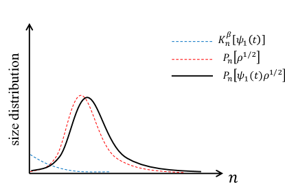
Pn[ψ1(t)ρ1/2]=(Kβ[ψ1(t)]P[ρ1/2])n=m=0nKmβ[ψ1(t)]Pnm[ρ1/2]subscript𝑃𝑛delimited-[]subscript𝜓1𝑡superscript𝜌12subscriptsuperscript𝐾𝛽delimited-[]subscript𝜓1𝑡𝑃delimited-[]superscript𝜌12𝑛superscriptsubscript𝑚0𝑛superscriptsubscript𝐾𝑚𝛽delimited-[]subscript𝜓1𝑡subscript𝑃𝑛𝑚delimited-[]superscript𝜌12P_{n}\left[\psi_{1}(t)\rho^{1/2}\right]=\left(K^{\beta}\left[\psi_{1}\left(t\right)\right]*P\left[\rho^{1/2}\right]\right)_{n}=\sum_{m=0}^{n}K_{m}^{\beta}\left[\psi_{1}(t)\right]P_{n-m}\left[\rho^{1/2}\right] (3.10)

with Kmβ[ψ1(t)]superscriptsubscript𝐾𝑚𝛽delimited-[]subscript𝜓1𝑡K_{m}^{\beta}\left[\psi_{1}(t)\right] defined by the expansion of 𝒢μ(β/4++it,β/4+it)subscript𝒢𝜇𝛽superscript4𝑖𝑡𝛽superscript4𝑖𝑡\mathcal{G}_{\mu}\left(\beta/4^{+}+it,\beta/4^{-}+it\right) in powers of eμsuperscript𝑒𝜇e^{-\mu}:

𝒢μ(β+4+it,β4+it)=m=0NemμKmβ[ψ1(t)]subscript𝒢𝜇superscript𝛽4𝑖𝑡superscript𝛽4𝑖𝑡superscriptsubscript𝑚0𝑁superscript𝑒𝑚𝜇superscriptsubscript𝐾𝑚𝛽delimited-[]subscript𝜓1𝑡\mathcal{G}_{\mu}\left(\frac{\beta^{+}}{4}+it,\frac{\beta^{-}}{4}+it\right)=\sum_{m=0}^{N}e^{-m\mu}K_{m}^{\beta}\left[\psi_{1}(t)\right] (3.11)

In this sense, Kmβsuperscriptsubscript𝐾𝑚𝛽K_{m}^{\beta} can be viewed as the “growth distribution” caused by applying ψ1(t)subscript𝜓1𝑡\psi_{1}(t) to the thermal state ρ1/2superscript𝜌12\rho^{1/2}.

Refer to caption
Figure 3: Schematic illustration of the size distribution Pn[ψ1(t)ρ1/2]subscript𝑃𝑛delimited-[]subscript𝜓1𝑡superscript𝜌12P_{n}\left[\psi_{1}\left(t\right)\rho^{1/2}\right] for the operator ψ1(t)ρ1/2subscript𝜓1𝑡superscript𝜌12\psi_{1}\left(t\right)\rho^{1/2} (black curve) which naturally decomposes into a convolution of a growth distribution Knβ[ψ1(t)]superscriptsubscript𝐾𝑛𝛽delimited-[]subscript𝜓1𝑡K_{n}^{\beta}\left[\psi_{1}\left(t\right)\right] (blue dashed curve) with the size distribution Pn[ρ1/2]subscript𝑃𝑛delimited-[]superscript𝜌12P_{n}\left[\rho^{1/2}\right] of the operator ρ1/2superscript𝜌12\rho^{1/2} (red dashed curve). This is due to the factorization relation of their respective generating functions (3.9).

Note that the discussion above can be generalized to arbitrary operators. For an arbitrary operator 𝒪𝒪\mathcal{O}, as long as we normalize it such that TFD|𝒪L𝒪L|TFD𝒪𝒪β=1quantum-operator-product𝑇𝐹𝐷superscriptsubscript𝒪𝐿subscript𝒪𝐿𝑇𝐹𝐷subscriptdelimited-⟨⟩superscript𝒪𝒪𝛽1\langle TFD|\mathcal{O}_{L}^{\dagger}\mathcal{O}_{L}|TFD\rangle\equiv\left\langle\mathcal{O}^{\dagger}\mathcal{O}\right\rangle_{\beta}=1, the expansion of the two-point function

𝒢μ[𝒪]𝒵μ[𝒪ρ1/2]𝒵μ[ρ1/2]subscript𝒢𝜇delimited-[]𝒪subscript𝒵𝜇delimited-[]𝒪superscript𝜌12subscript𝒵𝜇delimited-[]superscript𝜌12\mathcal{G}_{\mu}\left[\mathcal{O}\right]\equiv\frac{\mathcal{Z}_{\mu}\left[\mathcal{O}\rho^{1/2}\right]}{\mathcal{Z}_{\mu}\left[\rho^{1/2}\right]} (3.12)

measures the effective size distribution of 𝒪𝒪\mathcal{O} when applied to the thermal state.

3.3 Twisted Boundary Condition

We are interested in studying the generating function 𝒵μ[𝒪]subscript𝒵𝜇delimited-[]𝒪\mathcal{Z}_{\mu}\left[\mathcal{O}\right] for 𝒪=ρ1/2𝒪superscript𝜌12\mathcal{O}=\rho^{1/2} and 𝒪=ψ1(t)ρ1/2𝒪subscript𝜓1𝑡superscript𝜌12\mathcal{O}=\psi_{1}(t)\rho^{1/2}. As we discussed earlier, inserting the operator exp(μn)𝜇𝑛\exp\left(-\mu n\right) corresponds to changing the imaginary time evolution. The computation can be simplified by noticing that exp(μn)𝜇𝑛\exp\left(-\mu n\right) is a Gaussian operator, such that its action by conjugation to fermion operators ψiL,Rsuperscriptsubscript𝜓𝑖𝐿𝑅\psi_{i}^{L,R} leads to a simple linear superposition:

eμn(ψLiψR)eμn=(cosh(μ)sinh(μ)sinh(μ)cosh(μ))(ψLiψR)superscript𝑒𝜇𝑛superscript𝜓𝐿𝑖superscript𝜓𝑅superscript𝑒𝜇𝑛𝜇𝜇𝜇𝜇superscript𝜓𝐿𝑖superscript𝜓𝑅e^{\mu n}\left(\begin{array}[]{c}\psi^{L}\\ i\psi^{R}\end{array}\right)e^{-\mu n}=\left(\begin{array}[]{cc}\cosh\left(\mu\right)&-\sinh\left(\mu\right)\\ -\sinh\left(\mu\right)&\cosh\left(\mu\right)\end{array}\right)\left(\begin{array}[]{c}\psi^{L}\\ i\psi^{R}\end{array}\right) (3.13)

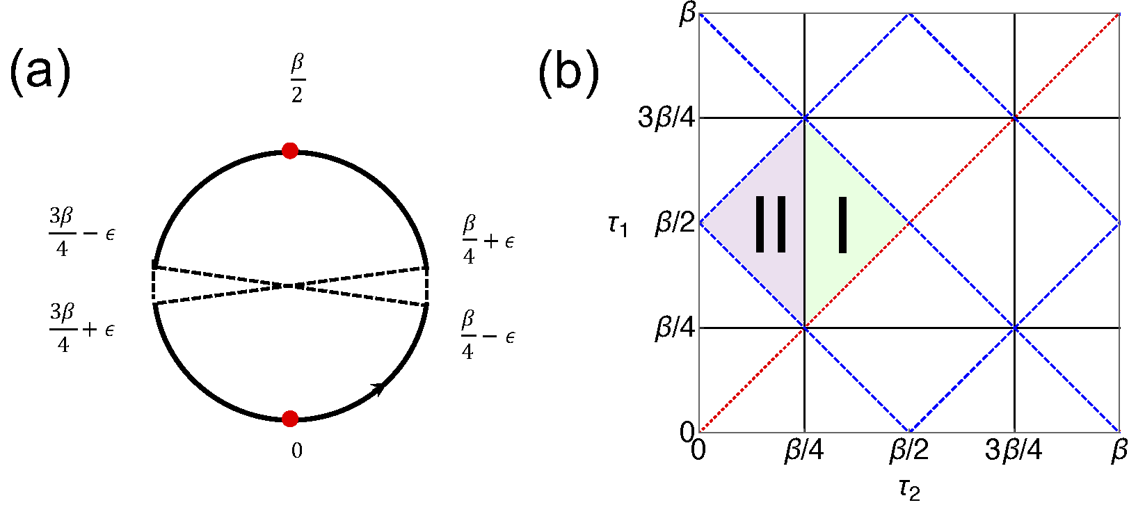
As a result, inserting the operator-weighting term exp(μn)𝜇𝑛\exp\left(-\mu n\right) is equivalent to twisting the boundary condition of the fermion fields at τ=β/4𝜏𝛽4\tau=\beta/4.

It is convenient to “de-purify” the system and return to the single copy of fermion fields, but with a twisted boundary condition. The single field is defined by continuously stitching the left and right fields together:

ψi(τ)={ψiL(τ)0τβ/2iψiR(βτ)β/2τ<βsubscript𝜓𝑖𝜏casessuperscriptsubscript𝜓𝑖𝐿𝜏0𝜏𝛽2𝑖superscriptsubscript𝜓𝑖𝑅𝛽𝜏𝛽2𝜏𝛽\psi_{i}\left(\tau\right)=\begin{cases}\psi_{i}^{L}\left(\tau\right)&0\leq\tau\leq\beta/2\\ i\psi_{i}^{R}\left(\beta-\tau\right)&\beta/2\leq\tau<\beta\end{cases} (3.14)

with the requirement of course that ψ(τ+β)=ψ(τ)𝜓𝜏𝛽𝜓𝜏\psi\left(\tau+\beta\right)=-\psi\left(\tau\right). This stitching transforms the purified action for the two fields into the original action for this single field; however, the twist condition must accompany the fields. In conclusion, the two-sided path integral in the presence of the factor exp(μn(β/4))𝜇𝑛𝛽4\exp\left(-\mu n\left(\beta/4\right)\right) equals the original path integral where the fields are twisted according to

limτβ/4+(ψ(τ)ψ(βτ))subscript𝜏𝛽superscript4𝜓𝜏𝜓𝛽𝜏\displaystyle\lim_{\tau\rightarrow\beta/4^{+}}\left(\begin{array}[]{c}\psi\left(\tau\right)\\ \psi\left(\beta-\tau\right)\end{array}\right) =(cosh(μ)sinh(μ)sinh(μ)cosh(μ))limτβ/4(ψ(τ)ψ(βτ))absent𝜇𝜇𝜇𝜇subscript𝜏𝛽superscript4𝜓𝜏𝜓𝛽𝜏\displaystyle=\left(\begin{array}[]{cc}\cosh\left(\mu\right)&-\sinh\left(\mu\right)\\ -\sinh\left(\mu\right)&\cosh\left(\mu\right)\end{array}\right)\lim_{\tau\rightarrow\beta/4^{-}}\left(\begin{array}[]{c}\psi\left(\tau\right)\\ \psi\left(\beta-\tau\right)\end{array}\right) (3.21)

Therefore, we conclude that calculating the two point function 𝒢μsubscript𝒢𝜇\mathcal{G}_{\mu} is equivalent to calculating the original two-point function, but with the following twisted boundary conditions

(limτ1/2β/4+𝒢μ(τ1,τ2)limτ1/23β/4𝒢μ(τ1,τ2))=(cosh(μ)sinh(μ)sinh(μ)cosh(μ))(limτ1/2β/4𝒢μ(τ1,τ2)limτ1/23β/4+𝒢μ(τ1,τ2))subscript𝜏12𝛽superscript4subscript𝒢𝜇subscript𝜏1subscript𝜏2subscript𝜏123𝛽superscript4subscript𝒢𝜇subscript𝜏1subscript𝜏2𝜇𝜇𝜇𝜇subscript𝜏12𝛽superscript4subscript𝒢𝜇subscript𝜏1subscript𝜏2subscript𝜏123𝛽superscript4subscript𝒢𝜇subscript𝜏1subscript𝜏2\left(\begin{array}[]{c}\underset{\tau_{1/2}\rightarrow\beta/4^{+}}{\lim}\mathcal{G}_{\mu}\left(\tau_{1},\tau_{2}\right)\\ \underset{\tau_{1/2}\rightarrow 3\beta/4^{-}}{\lim}\mathcal{G}_{\mu}\left(\tau_{1},\tau_{2}\right)\end{array}\right)=\left(\begin{array}[]{cc}\cosh\left(\mu\right)&-\sinh\left(\mu\right)\\ -\sinh\left(\mu\right)&\cosh\left(\mu\right)\end{array}\right)\left(\begin{array}[]{c}\underset{\tau_{1/2}\rightarrow\beta/4^{-}}{\lim}\mathcal{G}_{\mu}\left(\tau_{1},\tau_{2}\right)\\ \underset{\tau_{1/2}\rightarrow 3\beta/4^{+}}{\lim}\mathcal{G}_{\mu}\left(\tau_{1},\tau_{2}\right)\end{array}\right) (3.22)
Refer to caption
Figure 4: (a) The twisted boundary condition on the imaginary time circle. When τ𝜏\tau crosses β/4𝛽4\beta/4 from below, ψ(τ)𝜓𝜏\psi(\tau) becomes a superposition of ψ(β/4+ϵ)𝜓𝛽4italic-ϵ\psi\left(\beta/4+\epsilon\right) and ψ(3β/4ϵ)𝜓3𝛽4italic-ϵ\psi\left(3\beta/4-\epsilon\right) (see Eq. (3.21). (b) The various symmetry and boundary conditions on the twisted two point function in the (τ1,τ2)subscript𝜏1subscript𝜏2\left(\tau_{1},\tau_{2}\right) plane. First, 𝒢μsubscript𝒢𝜇\mathcal{G}_{\mu} is odd under reflections across the red dotted line and even under reflections across the blue dashed lines. Thus, it is sufficient to solve the saddle-point equations in the fundamental domain 0<τ1τ2<β/20subscript𝜏1subscript𝜏2𝛽20<\tau_{1}-\tau_{2}<\beta/2 and β/2<τ1+τ2<β𝛽2subscript𝜏1subscript𝜏2𝛽\beta/2<\tau_{1}+\tau_{2}<\beta. The black lines are the locations of the twisting boundary conditions (3.22), which reduce in the large q𝑞q limit (4.15) and divide our fundamental domain into two regions. Region I is where neither of the two fermions have crossed a twist, while in Region II the fermions are on opposite sides of the twist.

We note that while these conditions break time translation invariance, they preserve a set of discrete symmetries. Specifically, if the original Hamiltonian is time-reversal invariant, then 𝒢μ(τ1,τ2)subscript𝒢𝜇subscript𝜏1subscript𝜏2\mathcal{G}_{\mu}\left(\tau_{1},\tau_{2}\right) has reflection symmetry across the lines τ1±τ2=nβ/2plus-or-minussubscript𝜏1subscript𝜏2𝑛𝛽2\tau_{1}\pm\tau_{2}=n\beta/2 for all integers n𝑛n\in\mathbb{Z}

𝒢μ(τ1,τ2)=𝒢μ(nβ2τ2,nβ2τ1)=(1)n+1𝒢μ(τ2+nβ2,τ1nβ2)subscript𝒢𝜇subscript𝜏1subscript𝜏2subscript𝒢𝜇𝑛𝛽2subscript𝜏2𝑛𝛽2subscript𝜏1superscript1𝑛1subscript𝒢𝜇subscript𝜏2𝑛𝛽2subscript𝜏1𝑛𝛽2\mathcal{G}_{\mu}\left(\tau_{1},\tau_{2}\right)=\mathcal{G}_{\mu}\left(\frac{n\beta}{2}-\tau_{2},\frac{n\beta}{2}-\tau_{1}\right)=\left(-1\right)^{n+1}\mathcal{G}_{\mu}\left(\tau_{2}+\frac{n\beta}{2},\tau_{1}-\frac{n\beta}{2}\right) (3.23)

Thus, we need only to solve for 𝒢μ(τ1,τ2)subscript𝒢𝜇subscript𝜏1subscript𝜏2\mathcal{G}_{\mu}\left(\tau_{1},\tau_{2}\right) in the fundamental domain 0<τ1τ2<β/20subscript𝜏1subscript𝜏2𝛽20<\tau_{1}-\tau_{2}<\beta/2 and β/2<τ1+τ2<β𝛽2subscript𝜏1subscript𝜏2𝛽\beta/2<\tau_{1}+\tau_{2}<\beta, as shown in Fig. 4(b) by the union of regions I and II.

3.4 Thermally Renormalized Unit of Size

As an interesting application of our formalism, let us note how ψ1(t)subscript𝜓1𝑡\psi_{1}(t) affects ρ1/2superscript𝜌12\rho^{1/2} by taking t=0𝑡0t=0 and consider the change of average size by a single fermion operator ψ1subscript𝜓1\psi_{1}.

Δnβ[ψ1]Δsubscript𝑛𝛽delimited-[]subscript𝜓1\displaystyle\Delta n_{\beta}\left[\psi_{1}\right] n[ψ1ρ1/2]n[ρ1/2]absent𝑛delimited-[]subscript𝜓1superscript𝜌12𝑛delimited-[]superscript𝜌12\displaystyle\equiv n\left[\psi_{1}\rho^{1/2}\right]-n\left[\rho^{1/2}\right]
=12i=1N(TFD|ψ1LiψiLψiRψ1L|TFDTFD|iψiLψiR|TFD)absent12superscriptsubscript𝑖1𝑁quantum-operator-product𝑇𝐹𝐷superscriptsubscript𝜓1𝐿𝑖superscriptsubscript𝜓𝑖𝐿superscriptsubscript𝜓𝑖𝑅superscriptsubscript𝜓1𝐿𝑇𝐹𝐷quantum-operator-product𝑇𝐹𝐷𝑖superscriptsubscript𝜓𝑖𝐿superscriptsubscript𝜓𝑖𝑅𝑇𝐹𝐷\displaystyle=\frac{1}{2}\sum_{i=1}^{N}\left(\left\langle TFD\right|\psi_{1}^{L}i\psi_{i}^{L}\psi_{i}^{R}\psi_{1}^{L}\left|TFD\right\rangle-\left\langle TFD\right|i\psi_{i}^{L}\psi_{i}^{R}\left|TFD\right\rangle\right)
=TFD|iψ1Rψ1L|TFD=G11(β2)absentquantum-operator-product𝑇𝐹𝐷𝑖superscriptsubscript𝜓1𝑅superscriptsubscript𝜓1𝐿𝑇𝐹𝐷subscript𝐺11𝛽2\displaystyle=\left\langle TFD\right|i\psi_{1}^{R}\psi_{1}^{L}\left|TFD\right\rangle=G_{11}\left(\frac{\beta}{2}\right) (3.24)

At infinite temperature β0𝛽0\beta\rightarrow 0, G(β/2)=1𝐺𝛽21G\left(\beta/2\right)=1, which restores the trivial result that ψ1subscript𝜓1\psi_{1} increases the size of the density operator (which is proportional to identity operator, with size 00) by 111. At finite temperature, interestingly, the size change induced by a single fermion operator is smaller than 111, and is given by the same imaginary time two-point function as the one that determines the fractional scrambling distance δβ=1n[ρ1/2]N/2subscript𝛿𝛽1𝑛delimited-[]superscript𝜌12𝑁2\delta_{\beta}=1-\frac{n\left[\rho^{1/2}\right]}{N/2} in Eq. (3.3). In general, the size increase induced by ψisubscript𝜓𝑖\psi_{i} is Δnβ[ψi]=Gii(β/2)Δsubscript𝑛𝛽delimited-[]subscript𝜓𝑖subscript𝐺𝑖𝑖𝛽2\Delta n_{\beta}\left[\psi_{i}\right]=G_{ii}\left(\beta/2\right), which may depend on i𝑖i. The average size increase is exactly δβsubscript𝛿𝛽\delta_{\beta}. 222In term of the probabilities Kmβ[ψ1]superscriptsubscript𝐾𝑚𝛽delimited-[]subscript𝜓1K_{m}^{\beta}\left[\psi_{1}\right] in Eq. (3.11), we have Δn[ψi]=m=0NmKmβ[ψ1]Δ𝑛delimited-[]subscript𝜓𝑖superscriptsubscript𝑚0𝑁𝑚superscriptsubscript𝐾𝑚𝛽delimited-[]subscript𝜓1\Delta n\left[\psi_{i}\right]=\sum_{m=0}^{N}mK_{m}^{\beta}\left[\psi_{1}\right].

1NiΔn[ψi]=1NiGii(β2)=G(β2)=δβ1𝑁subscript𝑖Δ𝑛delimited-[]subscript𝜓𝑖1𝑁subscript𝑖subscript𝐺𝑖𝑖𝛽2𝐺𝛽2subscript𝛿𝛽\frac{1}{N}\sum_{i}\Delta n\left[\psi_{i}\right]=\frac{1}{N}\sum_{i}G_{ii}\left(\frac{\beta}{2}\right)=G\left(\frac{\beta}{2}\right)=\delta_{\beta} (3.25)

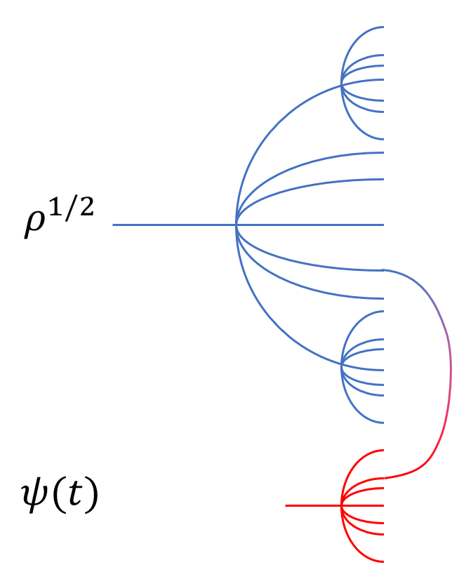
Physically, the average size change due to applying a single fermion is generically δβ<1subscript𝛿𝛽1\delta_{\beta}<1 at finite β𝛽\beta, because in the presence of a nontrivial ρ1/2superscript𝜌12\rho^{1/2} there is a chance that multiplying by ψ1subscript𝜓1\psi_{1} decreases the size, as is illustrated in Fig. 5, although the chance of increasing the size is always bigger. The closer the length of ρ1/2superscript𝜌12\rho^{1/2} is to the scrambling value n=N/2subscript𝑛𝑁2n_{*}=N/2, the smaller is the size increase Δnβ[ψ1ρ1/2]Δsubscript𝑛𝛽delimited-[]subscript𝜓1superscript𝜌12\Delta n_{\beta}\left[\psi_{1}\rho^{1/2}\right]. For a fully scrambled operator with n=N/2,δ=0formulae-sequence𝑛𝑁2𝛿0n=N/2,~{}\delta=0, multiplying a fermion ψ1subscript𝜓1\psi_{1} has equal chance of increasing or decreasing the size, so that the average size stays the same.
Refer to caption
Figure 5: At finite temperature, when an operator such as ψ1(t)subscript𝜓1𝑡\psi_{1}\left(t\right) is multiplied to ρ1/2superscript𝜌12\rho^{1/2}, there is a chance that some fermion flavors collide and the size increase is smaller than the size of ψ1(t)subscript𝜓1𝑡\psi_{1}\left(t\right) itself.

It should be emphasized that the discussion above is not restricted to the thermal density operator. For any operator 𝒪𝒪\mathcal{O}, we can define the size change

Δn𝒪[ψi]n[ψi𝒪]n[𝒪]Δsubscript𝑛𝒪delimited-[]subscript𝜓𝑖𝑛delimited-[]subscript𝜓𝑖𝒪𝑛delimited-[]𝒪\Delta n_{\mathcal{O}}\left[\psi_{i}\right]\equiv n\left[\psi_{i}\mathcal{O}\right]-n\left[\mathcal{O}\right] (3.26)

and obtain the following identity:

1NiΔn𝒪[ψi]=δ[𝒪]12n[𝒪]N1𝑁subscript𝑖Δsubscript𝑛𝒪delimited-[]subscript𝜓𝑖𝛿delimited-[]𝒪12𝑛delimited-[]𝒪𝑁\frac{1}{N}\sum_{i}\Delta n_{\mathcal{O}}\left[\psi_{i}\right]=\delta\left[\mathcal{O}\right]\equiv 1-\frac{2n\left[\mathcal{O}\right]}{N} (3.27)

The only thing special for the thermal density operator is the relation of ΔnΔ𝑛\Delta n to imaginary time two-point function in a single-copy system.

Furthermore, instead of ψisubscript𝜓𝑖\psi_{i} we can consider a string ΓIΓi1i2ik=ik(k1)2ψi1ψik1i1<i2<<ikNformulae-sequencesubscriptΓ𝐼subscriptΓsubscript𝑖1subscript𝑖2subscript𝑖𝑘superscript𝑖𝑘𝑘12subscript𝜓subscript𝑖1subscript𝜓subscript𝑖𝑘1subscript𝑖1subscript𝑖2subscript𝑖𝑘𝑁\Gamma_{I}\equiv\Gamma_{i_{1}i_{2}...i_{k}}=i^{\frac{k\left(k-1\right)}{2}}\psi_{i_{1}}...\psi_{i_{k}}\qquad 1\leq i_{1}<i_{2}<...<i_{k}\leq N introduced in Eq. (2.5), and consider how the size of ΓI𝒪subscriptΓ𝐼𝒪\Gamma_{I}\mathcal{O} is different from 𝒪𝒪\mathcal{O}. We have

Δn𝒪[ΓI]Δsubscript𝑛𝒪delimited-[]subscriptΓ𝐼\displaystyle\Delta n_{\mathcal{O}}\left[\Gamma_{I}\right] n[ΓI𝒪]n[𝒪]=s=1k𝒪|iψisRψisL|𝒪absent𝑛delimited-[]subscriptΓ𝐼𝒪𝑛delimited-[]𝒪superscriptsubscript𝑠1𝑘quantum-operator-product𝒪𝑖superscriptsubscript𝜓subscript𝑖𝑠𝑅superscriptsubscript𝜓subscript𝑖𝑠𝐿𝒪\displaystyle\equiv n\left[\Gamma_{I}\mathcal{O}\right]-n\left[\mathcal{O}\right]=\sum_{s=1}^{k}\left\langle\mathcal{O}\right|i\psi_{i_{s}}^{R}\psi_{i_{s}}^{L}\left|\mathcal{O}\right\rangle (3.28)

If we average over all Majorana strings ΓIsubscriptΓ𝐼\Gamma_{I} with the same size k𝑘k, we obtain

1CNkIΔn𝒪[ΓI]1superscriptsubscript𝐶𝑁𝑘subscript𝐼Δsubscript𝑛𝒪delimited-[]subscriptΓ𝐼\displaystyle\frac{1}{C_{N}^{k}}\sum_{I}\Delta n_{\mathcal{O}}\left[\Gamma_{I}\right] =kδ[𝒪]absent𝑘𝛿delimited-[]𝒪\displaystyle=k\delta\left[\mathcal{O}\right] (3.29)

In the last equation, CNk=N!k!(Nk)!superscriptsubscript𝐶𝑁𝑘𝑁𝑘𝑁𝑘C_{N}^{k}=\frac{N!}{k!(N-k)!} is the number of strings with length k𝑘k. This equation shows that the average size change induced by multiplying a string with length k𝑘k is k𝑘k times δ[𝒪]𝛿delimited-[]𝒪\delta\left[\mathcal{O}\right], further confirms that each fermion in the string contributes additively.

This observation suggests that at finite temperature (or more generally, for any density operator ρ𝜌\rho), the fractional scrambling distance δ𝛿\delta, rather than 111, should be considered as the fundamental unit of size, which is carried by each fermion operator. Indeed, as we will discuss in next section, our calculation in the SYK model in the large q𝑞q limit suggests universal behavior occurs when size is measured in this renormalized unit.

4 SYK Model

In this section, we will study the operator size growth in the SYK model [28, 29]. This model features q𝑞q-local interactions with independently random couplings, where each of the couplings is normal distributed

H=iq/21i1iqNJi1iqψi1ψiqJi1iq2=J2(N1q1)=𝒥22q(N1q1){ψi,ψj}=2δijformulae-sequenceformulae-sequence𝐻superscript𝑖𝑞2subscript1subscript𝑖1subscript𝑖𝑞𝑁subscript𝐽subscript𝑖1subscript𝑖𝑞subscript𝜓subscript𝑖1subscript𝜓subscript𝑖𝑞delimited-⟨⟩superscriptsubscript𝐽subscript𝑖1subscript𝑖𝑞2superscript𝐽2binomial𝑁1𝑞1superscript𝒥22𝑞binomial𝑁1𝑞1subscript𝜓𝑖subscript𝜓𝑗2subscript𝛿𝑖𝑗H=i^{q/2}\sum_{1\leq i_{1}...\leq i_{q}\leq N}J_{i_{1}...i_{q}}\psi_{i_{1}}...\psi_{i_{q}}\qquad\left\langle J_{i_{1}...i_{q}}^{2}\right\rangle=\frac{J^{2}}{\binom{N-1}{q-1}}=\frac{\mathcal{J}^{2}}{2q\binom{N-1}{q-1}}\qquad\left\{\psi_{i},\psi_{j}\right\}=2\delta_{ij} (4.1)

At large N𝑁N, the two-point function satisfies the saddle-point equations

[G]1superscriptdelimited-[]𝐺1\displaystyle\left[G\right]^{-1} =[G0]1[Σ]Σ(τ1,τ2)=𝒥22q(G(τ1,τ2))q1formulae-sequenceabsentsuperscriptdelimited-[]subscript𝐺01delimited-[]ΣΣsubscript𝜏1subscript𝜏2superscript𝒥22𝑞superscript𝐺subscript𝜏1subscript𝜏2𝑞1\displaystyle=[G_{0}]^{-1}-\left[\Sigma\right]\qquad\Sigma\left(\tau_{1},\tau_{2}\right)=\frac{\mathcal{J}^{2}}{2q}\left(G\left(\tau_{1},\tau_{2}\right)\right)^{q-1} (4.2)

where bracketed terms are Matsubara frequency matrices. One should note that since the fermions square to one, [G0]1=iω/2superscriptdelimited-[]subscript𝐺01𝑖𝜔2\left[G_{0}\right]^{-1}=-i\omega/2 rather than iω𝑖𝜔-i\omega.

4.1 Large q𝑞q Approximation

Refer to caption
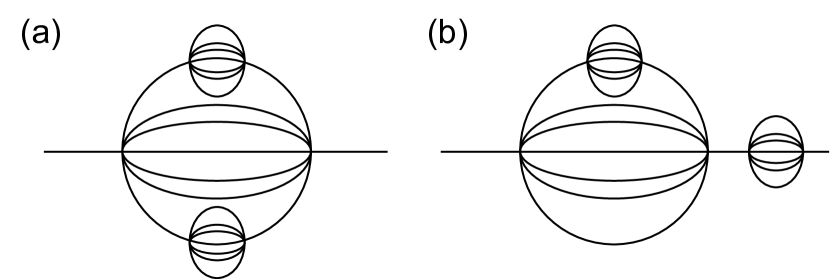
Figure 6: Two 𝒪(J6)𝒪superscript𝐽6\mathcal{O}\left(J^{6}\right) examples of the planar graphs of that survive the large-N𝑁N limit. Only graphs of form (a), where melons are inserted into melons, survive the large q𝑞q limit. Notice that there are 𝒪(q2)𝒪superscript𝑞2\mathcal{O}\left(q^{2}\right) graphs of form (a), while there are only 𝒪(q)𝒪𝑞\mathcal{O}\left(q\right) graphs of form (b). This is because there are 𝒪(q)𝒪𝑞\mathcal{O}\left(q\right) locations at any depth of a given graph to insert another melon; however, there are typically only 𝒪(1)𝒪1\mathcal{O}\left(1\right) locations to thread another melon. Accordingly, we take our coupling J𝐽J to equal 𝒥/2q𝒥2𝑞\mathcal{J}/\sqrt{2q}. Consequently, the 𝒪(q)𝒪𝑞\mathcal{O}\left(q\right) combinatorial enhancement gained for each new melon insertion is canceled by the J2=𝒥2/(2q)superscript𝐽2superscript𝒥22𝑞J^{2}=\mathcal{J}^{2}/\left(2q\right) factor accompanying said melon. This q𝑞q-scaling of the coupling isolates the infinite subset of the planar graphs where the graphs are two copies of a tree that are then glued together (a.k.a. “doubletree” graphs) such as (a). All non-doubletree graphs such as (b) are suppressed in q𝑞q since they receive factors of 𝒥2/(2q)superscript𝒥22𝑞\mathcal{J}^{2}/\left(2q\right) for each melon, but do not receive the necessary number of q𝑞q combinatorial enhancements.

In the language of Feynman diagrams, the Schwinger-Dyson equation (4.2) corresponds to only keeping the leading “melon diagrams” as is shown in Fig. 6. All other diagrams are sub-leading in large N𝑁N. In the large q𝑞q limit, there are two types of diagrams. Those with melons inserted into melons (such as Fig. 6(a)) receive a combinatorial q𝑞q enhancement, as there are many rungs upon which one may insert (hence the need for a q1superscript𝑞1q^{-1} factor in the self-energy to keep everything finite). In contrast, diagrams where melons are simply threaded together (such as Fig. 6(b)) do not receive this enhancement [35]. Thus, at large q𝑞q only the former dominate, which corresponds to the following truncation of the Schwinger-Dyson expansion:

[G]delimited-[]𝐺\displaystyle\left[G\right] =[G0]+[G0][Σ][G0]Σ(τ1,τ2)=𝒥22q(G(τ1,τ2))q1formulae-sequenceabsentdelimited-[]subscript𝐺0delimited-[]subscript𝐺0delimited-[]Σdelimited-[]subscript𝐺0Σsubscript𝜏1subscript𝜏2superscript𝒥22𝑞superscript𝐺subscript𝜏1subscript𝜏2𝑞1\displaystyle=\left[G_{0}\right]+\left[G_{0}\right]\left[\Sigma\right]\left[G_{0}\right]\qquad\Sigma\left(\tau_{1},\tau_{2}\right)=\frac{\mathcal{J}^{2}}{2q}\left(G\left(\tau_{1},\tau_{2}\right)\right)^{q-1}

Combing the equations together and Fourier transforming, one obtains

τ1τ2(GG0)=2𝒥2qGq1subscriptsubscript𝜏1subscriptsubscript𝜏2𝐺subscript𝐺02superscript𝒥2𝑞superscript𝐺𝑞1\partial_{\tau_{1}}\partial_{\tau_{2}}\left(G-G_{0}\right)=-\frac{2\mathcal{J}^{2}}{q}G^{q-1} (4.3)

The role played by G0subscript𝐺0G_{0} in this equation is to require that GG0𝐺subscript𝐺0G\rightarrow G_{0} as τ12subscript𝜏12\tau_{12} goes to integer multiples of β𝛽\beta. Therefore, if we take G=G0eσ/q𝐺subscript𝐺0superscript𝑒𝜎𝑞G=G_{0}e^{\sigma/q} with σ0𝜎0\sigma\rightarrow 0 at the τ12subscript𝜏12\tau_{12} boundaries, we obtain Liouville’s equation[30, 36]

τ1τ2σsubscriptsubscript𝜏1subscriptsubscript𝜏2𝜎\displaystyle\partial_{\tau_{1}}\partial_{\tau_{2}}\sigma =2𝒥2eσ+𝒪(1/q)absent2superscript𝒥2superscript𝑒𝜎𝒪1𝑞\displaystyle=-2\mathcal{J}^{2}e^{\sigma}+\mathcal{O}\left(1/q\right) (4.4)

where the field σ𝜎\sigma is expected to be periodic in both of its arguments, as well as have kinks when τ12subscript𝜏12\tau_{12} approaches integer multiples of β𝛽\beta.

Now in order to find 𝒢μsubscript𝒢𝜇\mathcal{G}_{\mu}, we will need to solve the above equations with the twisted boundary conditions (3.22). Furthermore, our twisted two-point function 𝒢μsubscript𝒢𝜇\mathcal{G}_{\mu} also satisfies the reflection conditions (3.23). Thus, we need only solve for 𝒢μsubscript𝒢𝜇\mathcal{G}_{\mu} in the fundamental domain 0<τ1τ2<β/20subscript𝜏1subscript𝜏2𝛽20<\tau_{1}-\tau_{2}<\beta/2 and β/2<τ1+τ2<β𝛽2subscript𝜏1subscript𝜏2𝛽\beta/2<\tau_{1}+\tau_{2}<\beta, as shown in Fig. 4(b) by the union of regions I and II.

4.2 The Large-q𝑞q solution

In the large q𝑞q limit, each commutator with the Hamiltonian increases the size of operator by qsimilar-toabsent𝑞\sim q, so that it is natural to measure the operator size in unit of q𝑞q. In the generating function, this corresponds to defining μ^qμ^𝜇𝑞𝜇\hat{\mu}\equiv q\mu (for reasons to be explained in the next subsection we will actually use the slightly smaller variable μ^=qδβμ^𝜇𝑞subscript𝛿𝛽𝜇\hat{\mu}=q\delta_{\beta}\mu (4.22)), with μ^^𝜇\hat{\mu} kept finite in the large q𝑞q limit. The derivative of the generating function over μ^^𝜇\hat{\mu} measures the size n𝑛n in unit of q𝑞q. If we consider the large q𝑞q limit with μ^^𝜇\hat{\mu} being kept finite, and use the large-q𝑞q ansatz for twisted two-point function

𝒢μ(τ1,τ2)=G0(τ1,τ2)eσμ(τ1,τ2)/q,subscript𝒢𝜇subscript𝜏1subscript𝜏2subscript𝐺0subscript𝜏1subscript𝜏2superscript𝑒subscript𝜎𝜇subscript𝜏1subscript𝜏2𝑞\mathcal{G}_{\mu}\left(\tau_{1},\tau_{2}\right)=G_{0}\left(\tau_{1},\tau_{2}\right)e^{\sigma_{\mu}\left(\tau_{1},\tau_{2}\right)/q}, (4.5)

the boundary condition (3.22) reduces to

(limτ1/2β/4+𝒢μ(τ1,τ2)limτ1/23β/4𝒢μ(τ1,τ2))subscript𝜏12𝛽superscript4subscript𝒢𝜇subscript𝜏1subscript𝜏2subscript𝜏123𝛽superscript4subscript𝒢𝜇subscript𝜏1subscript𝜏2\displaystyle\left(\begin{array}[]{c}\underset{\tau_{1/2}\rightarrow\beta/4^{+}}{\lim}\mathcal{G}_{\mu}\left(\tau_{1},\tau_{2}\right)\\ \underset{\tau_{1/2}\rightarrow 3\beta/4^{-}}{\lim}\mathcal{G}_{\mu}\left(\tau_{1},\tau_{2}\right)\end{array}\right) (1μ^qμ^q1)(limτ1/2β/4𝒢μ(τ1,τ2)limτ1/23β/4+𝒢μ(τ1,τ2))similar-to-or-equalsabsent1^𝜇𝑞^𝜇𝑞1subscript𝜏12𝛽superscript4subscript𝒢𝜇subscript𝜏1subscript𝜏2subscript𝜏123𝛽superscript4subscript𝒢𝜇subscript𝜏1subscript𝜏2\displaystyle\simeq\left(\begin{array}[]{cc}1&-\frac{\hat{\mu}}{q}\\ -\frac{\hat{\mu}}{q}&1\end{array}\right)\left(\begin{array}[]{c}\underset{\tau_{1/2}\rightarrow\beta/4^{-}}{\lim}\mathcal{G}_{\mu}\left(\tau_{1},\tau_{2}\right)\\ \underset{\tau_{1/2}\rightarrow 3\beta/4^{+}}{\lim}\mathcal{G}_{\mu}\left(\tau_{1},\tau_{2}\right)\end{array}\right) (4.12)
eμ^/q(limτ1/2β/4𝒢μ(τ1,τ2)limτ1/23β/4+𝒢μ(τ1,τ2))similar-to-or-equalsabsentsuperscript𝑒^𝜇𝑞subscript𝜏12𝛽superscript4subscript𝒢𝜇subscript𝜏1subscript𝜏2subscript𝜏123𝛽superscript4subscript𝒢𝜇subscript𝜏1subscript𝜏2\displaystyle\simeq e^{-\hat{\mu}/q}\left(\begin{array}[]{c}\underset{\tau_{1/2}\rightarrow\beta/4^{-}}{\lim}\mathcal{G}_{\mu}\left(\tau_{1},\tau_{2}\right)\\ \underset{\tau_{1/2}\rightarrow 3\beta/4^{+}}{\lim}\mathcal{G}_{\mu}\left(\tau_{1},\tau_{2}\right)\end{array}\right) (4.15)

Thus, to the leading order of 1q1𝑞\frac{1}{q}, the two equations for β/4𝛽4\beta/4 and 3β/43𝛽43\beta/4 decouple.

As a reminder, these equations encode the effect of moving a Majorana fermion on the Euclidean circle (i.e. the two TFD half-circles) from one side of the twist operator (3.8) to the other. The factor of exp(μ^/q)=exp(μ)^𝜇𝑞𝜇\exp\left(-\hat{\mu}/q\right)=\exp\left(-\mu\right) denotes the fact that such an action changes the size of the doubled state by exactly one whole fermion. However, we shall find that for states of large size such as the thermofield double (i.e. Gibbs state) each Majorana fermion actually increases the total average operator size by a smaller fraction δβsubscript𝛿𝛽\delta_{\beta} rather than 111, where the size change δβsubscript𝛿𝛽\delta_{\beta} is smaller when the state’s size is larger. As such, we shall find that it will be appropriate to use the variable μ^=qμδβ^𝜇𝑞𝜇subscript𝛿𝛽\hat{\mu}=q\mu\delta_{\beta} instead of μ^=qμ^𝜇𝑞𝜇\hat{\mu}=q\mu when taking the large-q𝑞q limit.

The twisted two-point function in large-q𝑞q limit can thus be obtained by solving Liouville’s equation (4.4) with the μ𝜇\mu-dependent boundary conditions (4.15). Here we will skip the tedious details and directly present the solution. When the times are such that the two fermions are on the same side of the twisted boundary, which corresponds to τ2>β/4subscript𝜏2𝛽4\tau_{2}>\beta/4 (region I in Fig. 4(b), we find a seemingly time-translation invariant solution solution

𝒢μ(τ1,τ2)subscript𝒢𝜇subscript𝜏1subscript𝜏2\displaystyle\mathcal{G}_{\mu}\left(\tau_{1},\tau_{2}\right) =(sinγμsin(αμ(τ1τ2)+γμ))2/qGμ(τ1τ2)absentsuperscriptsubscript𝛾𝜇subscript𝛼𝜇subscript𝜏1subscript𝜏2subscript𝛾𝜇2𝑞subscript𝐺𝜇subscript𝜏1subscript𝜏2\displaystyle=\left(\frac{\sin\gamma_{\mu}}{\sin\left(\alpha_{\mu}\left(\tau_{1}-\tau_{2}\right)+\gamma_{\mu}\right)}\right)^{2/q}\equiv G_{\mu}\left(\tau_{1}-\tau_{2}\right) (4.16)

However, when the times are such that the two fermions are on opposite sides of the twisted boundary at β/4𝛽4\beta/4 and 3β/43𝛽43\beta/4, which for our domain amounts to the condition τ2<β/4subscript𝜏2𝛽4\tau_{2}<\beta/4 (region II in Fig. 4(b), the time translation symmetry is explicitly broken

𝒢μ(τ1,τ2)subscript𝒢𝜇subscript𝜏1subscript𝜏2\displaystyle\mathcal{G}_{\mu}\left(\tau_{1},\tau_{2}\right) =eμ^/qGμ(τ1τ2)(1(1eμ^)sin2γμ(Gμ(τ1τ2))q/2sin(αμ(τ1β4))sin(αμ(τ2β4)))2/qabsentsuperscript𝑒^𝜇𝑞subscript𝐺𝜇subscript𝜏1subscript𝜏2superscript11superscript𝑒^𝜇superscript2subscript𝛾𝜇superscriptsubscript𝐺𝜇subscript𝜏1subscript𝜏2𝑞2subscript𝛼𝜇subscript𝜏1𝛽4subscript𝛼𝜇subscript𝜏2𝛽42𝑞\displaystyle=\frac{e^{-\hat{\mu}/q}G_{\mu}\left(\tau_{1}-\tau_{2}\right)}{\left(1-\frac{\left(1-e^{-\hat{\mu}}\right)}{\sin^{2}\gamma_{\mu}}\left(G_{\mu}\left(\tau_{1}-\tau_{2}\right)\right)^{q/2}\sin\left(\alpha_{\mu}\left(\tau_{1}-\frac{\beta}{4}\right)\right)\sin\left(\alpha_{\mu}\left(\tau_{2}-\frac{\beta}{4}\right)\right)\right)^{2/q}} (4.17)

Here the parameters αμsubscript𝛼𝜇\alpha_{\mu} and γμsubscript𝛾𝜇\gamma_{\mu} are functions of β𝒥𝛽𝒥\beta\mathcal{J} and μ𝜇\mu, which are determined by the boundary condition 𝒢(τ,τ)=1𝒢𝜏𝜏1\mathcal{G}(\tau,\tau)=1 as well as the reflection conditions (3.23)

αμβsubscript𝛼𝜇𝛽\displaystyle\alpha_{\mu}\beta =β𝒥sinγμ,sin(αμβ2+2γμ)=eμ^sin(αμβ2)formulae-sequenceabsent𝛽𝒥subscript𝛾𝜇subscript𝛼𝜇𝛽22subscript𝛾𝜇superscript𝑒^𝜇subscript𝛼𝜇𝛽2\displaystyle=\beta\mathcal{J}\sin\gamma_{\mu},\quad\sin\left(\frac{\alpha_{\mu}\beta}{2}+2\gamma_{\mu}\right)=e^{-\hat{\mu}}\sin\left(\frac{\alpha_{\mu}\beta}{2}\right) (4.18)

In the limit μ0𝜇0\mu\rightarrow 0, we recover the untwisted two-point function 𝒢μ=0(τ1,τ2)=Gμ=0(τ1τ2)=G(τ1τ2)subscript𝒢𝜇0subscript𝜏1subscript𝜏2subscript𝐺𝜇0subscript𝜏1subscript𝜏2𝐺subscript𝜏1subscript𝜏2\mathcal{G}_{\mu=0}(\tau_{1},\tau_{2})=G_{\mu=0}(\tau_{1}-\tau_{2})=G\left(\tau_{1}-\tau_{2}\right) in the whole domain, and the equation for the parameters reduce to the ordinary case[30]:

αμ=0α=𝒥cos(αβ2),γμ=0γ=παβ2formulae-sequencesubscript𝛼𝜇0𝛼𝒥𝛼𝛽2subscript𝛾𝜇0𝛾𝜋𝛼𝛽2\alpha_{\mu=0}\equiv\alpha=\mathcal{J}\cos\left(\frac{\alpha\beta}{2}\right),\quad\gamma_{\mu=0}\equiv\gamma=\frac{\pi-\alpha\beta}{2} (4.19)

The asymptotic behavior at small values of β𝒥𝛽𝒥\beta\mathcal{J} and large values of β𝒥𝛽𝒥\beta\mathcal{J} respectively are given by

α𝛼\displaystyle\alpha =𝒥(1β2𝒥28+𝒪(β4𝒥4))absent𝒥1superscript𝛽2superscript𝒥28𝒪superscript𝛽4superscript𝒥4\displaystyle=\mathcal{J}\left(1-\frac{\beta^{2}\mathcal{J}^{2}}{8}+\mathcal{O}\left(\beta^{4}\mathcal{J}^{4}\right)\right) α𝛼\displaystyle\alpha =πβ(12β𝒥+𝒪(1β2𝒥2))absent𝜋𝛽12𝛽𝒥𝒪1superscript𝛽2superscript𝒥2\displaystyle=\frac{\pi}{\beta}\left(1-\frac{2}{\beta\mathcal{J}}+\mathcal{O}\left(\frac{1}{\beta^{2}\mathcal{J}^{2}}\right)\right)

4.3 Size renormalization

Before carrying further analysis to the SYK operator growth in next section, we need to discuss an important modification to the two-point function solution due to higher order q𝑞q effects. If we take τ1β/4+ϵ,τ2β/4ϵformulae-sequencesubscript𝜏1𝛽4italic-ϵsubscript𝜏2𝛽4italic-ϵ\tau_{1}\rightarrow\beta/4+\epsilon,~{}\tau_{2}\rightarrow\beta/4-\epsilon in Eq. (4.17), we obtain

𝒢μ(β4+ϵ,β4ϵ)=eμ^/qsubscript𝒢𝜇𝛽4italic-ϵ𝛽4italic-ϵsuperscript𝑒^𝜇𝑞\mathcal{G}_{\mu}\left(\frac{\beta}{4}+\epsilon,\frac{\beta}{4}-\epsilon\right)=e^{-\hat{\mu}/q} (4.20)

This is the kernel that determines the size change induced by multiplying ψ1subscript𝜓1\psi_{1} to ρ1/2superscript𝜌12\rho^{1/2}, which has been discussed in section (3.4). Taking the μ𝜇\mu-derivative of 𝒢μsubscript𝒢𝜇\mathcal{G}_{\mu}, we find

Δnβ[ψ1]Δsubscript𝑛𝛽delimited-[]subscript𝜓1\displaystyle\Delta n_{\beta}\left[\psi_{1}\right] n[ψ1ρ1/2]n[ρ1/2]=μlog𝒢μ(β4+ϵ,β4ϵ)|μ=0=1absent𝑛delimited-[]subscript𝜓1superscript𝜌12𝑛delimited-[]superscript𝜌12evaluated-atsubscript𝜇subscript𝒢𝜇𝛽4italic-ϵ𝛽4italic-ϵ𝜇01\displaystyle\equiv n\left[\psi_{1}\rho^{1/2}\right]-n\left[\rho^{1/2}\right]=-\left.\partial_{\mu}\log\mathcal{G}_{\mu}\left(\frac{\beta}{4}+\epsilon,\frac{\beta}{4}-\epsilon\right)\right|_{\mu=0}=1

However, we also know that the size change is directly determined by the two-point function due to Eq. (3.24):

Δnβ[ψ1]=δβ=G(β2)=(α𝒥)2/qΔsubscript𝑛𝛽delimited-[]subscript𝜓1subscript𝛿𝛽𝐺𝛽2superscript𝛼𝒥2𝑞\Delta n_{\beta}\left[\psi_{1}\right]=\delta_{\beta}=G\left(\frac{\beta}{2}\right)=\left(\frac{\alpha}{\mathcal{J}}\right)^{2/q} (4.21)

where ααμ=0(β𝒥)𝛼subscript𝛼𝜇0𝛽𝒥\alpha\equiv\alpha_{\mu=0}\left(\beta\mathcal{J}\right) is the smallest positive root of Eq. (4.19).

This discrepancy between the two calculations is because δβ1subscript𝛿𝛽1\delta_{\beta}\rightarrow 1 in the large q𝑞q limit, and the 𝒪(q1)𝒪superscript𝑞1\mathcal{O}\left(q^{-1}\right) difference is neglected in the approximation we made to the boundary condition. The easiest way to resolve this issue and makes a consistent large-q𝑞q limit is by redefining μ^=qμ^𝜇𝑞𝜇\hat{\mu}=q\mu to

μ^=qμδβ^𝜇𝑞𝜇subscript𝛿𝛽\hat{\mu}=q\mu\delta_{\beta} (4.22)

in Eq. (4.15), which leads to the same substitution in Eqs. (4.16), (4.17), and (4.18). In the following, we will always use this definition of μ^^𝜇\hat{\mu}.

Physically, this substitution is a consequence of the size renormalization discussed in section (3.4). Each Majorana fermion increase the operator size by δβsubscript𝛿𝛽\delta_{\beta} rather than 111. Each action of the Hamiltonian increases the operator size by qδβsimilar-toabsent𝑞subscript𝛿𝛽\sim q\delta_{\beta}. Although in large q𝑞q limit 1δβ1subscript𝛿𝛽1-\delta_{\beta} is order q1superscript𝑞1q^{-1}, it is important to keep track of this distance, since the same δβsubscript𝛿𝛽\delta_{\beta} also measures the fractional scrambling distance of ρ1/2superscript𝜌12\rho^{1/2}, as we discussed in section (3.1). The size of ρ1/2superscript𝜌12\rho^{1/2} is

n[ρ1/2]=N2(1δβ)=N2(1(α𝒥)2/q)𝑛delimited-[]superscript𝜌12𝑁21subscript𝛿𝛽𝑁21superscript𝛼𝒥2𝑞n\left[\rho^{1/2}\right]=\frac{N}{2}\left(1-\delta_{\beta}\right)=\frac{N}{2}\left(1-\left(\frac{\alpha}{\mathcal{J}}\right)^{2/q}\right) (4.23)

which decreases with increasing q𝑞q, but is always large since we should always take the large N𝑁N limit before taking large q𝑞q.

5 SYK Operator Growth

We are now equipped with everything we need to understand Pn[ψ1(t)ρ1/2]subscript𝑃𝑛delimited-[]subscript𝜓1𝑡superscript𝜌12P_{n}\left[\psi_{1}\left(t\right)\rho^{1/2}\right], the size distribution of ψ1(t)ρ1/2subscript𝜓1𝑡superscript𝜌12\psi_{1}\left(t\right)\rho^{1/2}. According to Eq. (3.9), the generating function 𝒵μ[ψ1(t)ρ1/2]subscript𝒵𝜇delimited-[]subscript𝜓1𝑡superscript𝜌12\mathcal{Z}_{\mu}\left[\psi_{1}(t)\rho^{1/2}\right] for this distribution splits into a product of the thermal state’s generating function 𝒵μ[ρ1/2]subscript𝒵𝜇delimited-[]superscript𝜌12\mathcal{Z}_{\mu}\left[\rho^{1/2}\right] and 𝒢μ(β/4++it,β/4+it)subscript𝒢𝜇𝛽superscript4𝑖𝑡𝛽superscript4𝑖𝑡\mathcal{G}_{\mu}\left(\beta/4^{+}+it,\beta/4^{-}+it\right). The latter is simply the twisted two-point function we discussed in the previous subsection with an analytic continuation.

5.1 Thermal State

The generating function 𝒵μ[ρ1/2]subscript𝒵𝜇delimited-[]superscript𝜌12\mathcal{Z}_{\mu}\left[\rho^{1/2}\right] is the partition function of the system with the insertion exp(μn(β/4))𝜇𝑛𝛽4\exp\left(-\mu n\left(\beta/4\right)\right) divided by that of the original system (see Eq. (3.5)). This quantity can be determined by the twisted two-point function, since one has

μln𝒵μsubscript𝜇subscript𝒵𝜇\displaystyle-\partial_{\mu}\ln\mathcal{Z}_{\mu} =ρ1/2|neμn|ρ1/2ρ1/2|eμn|ρ1/2=N2(1Gμ(β2))=N2(1sin2/qγμsin2/q(αμβ2+γμ))absentexpectation-value𝑛superscript𝑒𝜇𝑛superscript𝜌12superscript𝜌12expectation-valuesuperscript𝑒𝜇𝑛superscript𝜌12superscript𝜌12𝑁21subscript𝐺𝜇𝛽2𝑁21superscript2𝑞subscript𝛾𝜇superscript2𝑞subscript𝛼𝜇𝛽2subscript𝛾𝜇\displaystyle=\frac{\expectationvalue*{ne^{-\mu n}}{\rho^{1/2}}}{\expectationvalue*{e^{-\mu n}}{\rho^{1/2}}}=\frac{N}{2}\left(1-G_{\mu}\left(\frac{\beta}{2}\right)\right)=\frac{N}{2}\left(1-\frac{\sin^{2/q}\gamma_{\mu}}{\sin^{2/q}\left(\alpha_{\mu}\frac{\beta}{2}+\gamma_{\mu}\right)}\right)

In theory, we can integrate this equation to obtain 𝒵μ[ρ1/2]subscript𝒵𝜇delimited-[]superscript𝜌12\mathcal{Z}_{\mu}\left[\rho^{1/2}\right]. However, many important properties of the distribution can be inferred from just the first and second moment.

The first moment is simply the average size

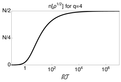
n[ρ1/2]=N2(1δβ)=N2(1G(β2))=N2(1(α𝒥)2/q)𝑛delimited-[]superscript𝜌12𝑁21subscript𝛿𝛽𝑁21𝐺𝛽2𝑁21superscript𝛼𝒥2𝑞n\left[\rho^{1/2}\right]=\frac{N}{2}\left(1-\delta_{\beta}\right)=\frac{N}{2}\left(1-G\left(\frac{\beta}{2}\right)\right)=\frac{N}{2}\left(1-\left(\frac{\alpha}{\mathcal{J}}\right)^{2/q}\right) (5.1)

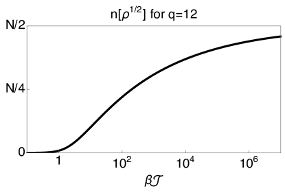
The behavior of n[ρ1/2]𝑛delimited-[]superscript𝜌12n\left[\rho^{1/2}\right] for two different q𝑞q values are plotted in Fig. 7 as a function of β𝒥𝛽𝒥\beta\mathcal{J}. Interestingly, we see that for larger q𝑞q it takes larger values of β𝒥𝛽𝒥\beta\mathcal{J} to achieve the same average size. Thus, the exponentiation of increasingly heavy SYK Hamiltonians results in relatively lighter thermal states. This is unintuitive, so one might argue that it is simply due to the q𝑞q-scaling nature of 𝒥𝒥\mathcal{J}, but that is only a constant shift in the log scale plot in Fig. 7, which is nowhere large enough to account for the above discrepancy. The true origin of this effect is the power of 2/q2𝑞2/q in the two-point function. We conclude that this heavy-light relationship is thus a non-trivial consequence of the large-N𝑁N and large-q𝑞q limit.

Refer to caption
Refer to caption
Figure 7: Plots of the average size of ρ1/2exp(βH/2)proportional-tosuperscript𝜌12𝛽𝐻2\rho^{1/2}\propto\exp\left(-\beta H/2\right) for different q𝑞q, given by Eq. (5.1).

For β𝒥eqmuch-greater-than𝛽𝒥superscript𝑒𝑞\beta\mathcal{J}\gg e^{q}, one expects that the higher order corrections to Liouville’s equation (4.4) cannot be neglected, and so one should turn to the conformal approximation[30]. Their expression for the two-point function implies that the average size of ρ1/2superscript𝜌12\rho^{1/2} when Nβ𝒥1much-greater-than𝑁𝛽𝒥much-greater-than1N\gg\beta\mathcal{J}\gg 1 is given by

n[ρ1/2]𝑛delimited-[]superscript𝜌12\displaystyle n\left[\rho^{1/2}\right] N2(1c(q)(πβ𝒥)2/q)absent𝑁21𝑐𝑞superscript𝜋𝛽𝒥2𝑞\displaystyle\approx\frac{N}{2}\left(1-c\left(q\right)\left(\frac{\pi}{\beta\mathcal{J}}\right)^{2/q}\right) c(q)𝑐𝑞\displaystyle c\left(q\right) =((q2)tanπqπ)1/qabsentsuperscript𝑞2𝜋𝑞𝜋1𝑞\displaystyle=\left(\frac{\left(q-2\right)\tan\frac{\pi}{q}}{\pi}\right)^{1/q}

The difference between the large q𝑞q and low temperature n[ρ1/2]=N2(1G(β2))𝑛delimited-[]superscript𝜌12𝑁21𝐺𝛽2n\left[\rho^{1/2}\right]=\frac{N}{2}\left(1-G\left(\frac{\beta}{2}\right)\right) is captured by the factor c(q)𝑐𝑞c\left(q\right). It monotonically increases from c(4)=(2/π)1/40.9𝑐4superscript2𝜋140.9c\left(4\right)=\left(2/\pi\right)^{1/4}\approx 0.9 when q=4𝑞4q=4, and asymptotically approaches 111 when q𝑞q is large as 12/q212superscript𝑞21-2/q^{2}. We expect that q=4𝑞4q=4 and large β𝒥𝛽𝒥\beta\mathcal{J} will be where our large q𝑞q approximation will have the largest error. However, that this error is at worst 10%percent1010\% renews our confidence that the large q𝑞q approximation captures important analytic features of the large-N𝑁N SYK model.

The second derivative of ln𝒵μsubscript𝒵𝜇\ln\mathcal{Z}_{\mu} determines the width of the distribution:

σn2[ρ1/2]superscriptsubscript𝜎𝑛2delimited-[]superscript𝜌12\displaystyle\sigma_{n}^{2}\left[\rho^{1/2}\right] =limμ0μ2ln𝒵μ[ρ1/2]=N2μGμ(β2)|μ0Nabsentsubscript𝜇0superscriptsubscript𝜇2subscript𝒵𝜇delimited-[]superscript𝜌12evaluated-at𝑁2subscript𝜇subscript𝐺𝜇𝛽2𝜇0proportional-to𝑁\displaystyle=\lim_{\mu\rightarrow 0}\partial_{\mu}^{2}\ln\mathcal{Z}_{\mu}\left[\rho^{1/2}\right]=\frac{N}{2}\left.\partial_{\mu}G_{\mu}\left(\frac{\beta}{2}\right)\right|_{\mu\rightarrow 0}\propto N

Therefore the width of the distribution σnNproportional-tosubscript𝜎𝑛𝑁\sigma_{n}\propto\sqrt{N}, such that the relative deviation from the average value σn[ρ1/2]/n[ρ1/2]N1/2proportional-tosubscript𝜎𝑛delimited-[]superscript𝜌12𝑛delimited-[]superscript𝜌12superscript𝑁12\sigma_{n}\left[\rho^{1/2}\right]/n\left[\rho^{1/2}\right]\propto N^{-1/2} is sharply peaked in the large N𝑁N limit. This is a consequence of large N𝑁N factorization.

5.2 Thermal Fermion

As explicitly discussed in section (3.2), the generating function for the growth distribution Kβsuperscript𝐾𝛽K^{\beta} (3.11) is determined by the twisted two-point function (4.17)

𝒢μ(β+4+it,β4+it)subscript𝒢𝜇superscript𝛽4𝑖𝑡superscript𝛽4𝑖𝑡\displaystyle\mathcal{G}_{\mu}\left(\frac{\beta^{+}}{4}+it,\frac{\beta^{-}}{4}+it\right) =eμδβ(1+(1eqμδβ)(𝒥αμsinhαμt)2)2/qabsentsuperscript𝑒𝜇subscript𝛿𝛽superscript11superscript𝑒𝑞𝜇subscript𝛿𝛽superscript𝒥subscript𝛼𝜇subscript𝛼𝜇𝑡22𝑞\displaystyle=e^{-\mu\delta_{\beta}}\left(1+\left(1-e^{-q\mu\delta_{\beta}}\right)\left(\frac{\mathcal{J}}{\alpha_{\mu}}\sinh\alpha_{\mu}t\right)^{2}\right)^{-2/q}

where αμsubscript𝛼𝜇\alpha_{\mu} and γμsubscript𝛾𝜇\gamma_{\mu} depend on μ𝜇\mu and β𝒥𝛽𝒥\beta\mathcal{J} through the constraints (4.18).

5.2.1 Average Size

This implies that the average size of the operator ψ(t)ρ1/2𝜓𝑡superscript𝜌12\psi\left(t\right)\rho^{1/2} is given by

n[ψ1(t)ρ1/2]𝑛delimited-[]subscript𝜓1𝑡superscript𝜌12\displaystyle n\left[\psi_{1}\left(t\right)\rho^{1/2}\right] =n[ρ1/2]μln𝒢μ(β+4+it,β4+it)|μ=0absent𝑛delimited-[]superscript𝜌12evaluated-atsubscript𝜇subscript𝒢𝜇superscript𝛽4𝑖𝑡superscript𝛽4𝑖𝑡𝜇0\displaystyle=n\left[\rho^{1/2}\right]-\left.\partial_{\mu}\ln\mathcal{G}_{\mu}\left(\frac{\beta^{+}}{4}+it,\frac{\beta^{-}}{4}+it\right)\right|_{\mu=0}
n[ψ1(t)ρ1/2]absent𝑛delimited-[]subscript𝜓1𝑡superscript𝜌12\displaystyle\Rightarrow n\left[\psi_{1}\left(t\right)\rho^{1/2}\right] =N2(1δβ)+δβ(1+2(𝒥αsinhαt)2)absent𝑁21subscript𝛿𝛽subscript𝛿𝛽12superscript𝒥𝛼𝛼𝑡2\displaystyle=\frac{N}{2}\left(1-\delta_{\beta}\right)+\delta_{\beta}\left(1+2\left(\frac{\mathcal{J}}{\alpha}\sinh\alpha t\right)^{2}\right) (5.2)

where δβ=(α/𝒥)2/qsubscript𝛿𝛽superscript𝛼𝒥2𝑞\delta_{\beta}=\left(\alpha/\mathcal{J}\right)^{2/q}, and ααμ=0(β𝒥)𝛼subscript𝛼𝜇0𝛽𝒥\alpha\equiv\alpha_{\mu=0}\left(\beta\mathcal{J}\right) is the smallest positive root of Eq. (4.19). We see that the difference in averages sizes of ψ(t)ρ1/2𝜓𝑡superscript𝜌12\psi\left(t\right)\rho^{1/2} and ρ1/2superscript𝜌12\rho^{1/2} is a simple when expressed in the renormalized size unit δβsubscript𝛿𝛽\delta_{\beta}, which inspires us to define a notion of the “average growth” of ψ1(t)subscript𝜓1𝑡\psi_{1}\left(t\right) as

Δn~β[ψ1(t)]n[ψ1(t)ρ1/2]n[ρ1/2]δβ=1+2(𝒥αsinhαt)2Δsubscript~𝑛𝛽delimited-[]subscript𝜓1𝑡𝑛delimited-[]subscript𝜓1𝑡superscript𝜌12𝑛delimited-[]superscript𝜌12subscript𝛿𝛽12superscript𝒥𝛼𝛼𝑡2\Delta\tilde{n}_{\beta}\left[\psi_{1}(t)\right]\equiv\frac{n\left[\psi_{1}(t)\rho^{1/2}\right]-n\left[\rho^{1/2}\right]}{\delta_{\beta}}=1+2\left(\frac{\mathcal{J}}{\alpha}\sinh\alpha t\right)^{2} (5.3)

Now, scrambling occurs when the average size of ψ1(t)ρ1/2subscript𝜓1𝑡superscript𝜌12\psi_{1}\left(t\right)\rho^{1/2} given by Eq. (5.2) reaches n=N/2subscript𝑛𝑁2n_{*}=N/2. This produces a slightly complicated expression for the scrambling time tsubscript𝑡t_{*}; however, it simplifies dramatically when phrased in terms of the average growth of ψ1(t)subscript𝜓1𝑡\psi_{1}\left(t\right). Manipulating the scrambling time equation n[ψ1(t)ρ1/2]=N/2𝑛delimited-[]subscript𝜓1subscript𝑡superscript𝜌12𝑁2n\left[\psi_{1}\left(t_{*}\right)\rho^{1/2}\right]=N/2, we find that one may equivalently state that scrambling occurs when the average growth of ψ1(t)subscript𝜓1𝑡\psi_{1}\left(t\right) reaches n=N/2subscript𝑛𝑁2n_{*}=N/2

Δn~β[ψ1(t)]=1+2(𝒥αsinhαt)2=N2Δsubscript~𝑛𝛽delimited-[]subscript𝜓1subscript𝑡12superscript𝒥𝛼𝛼subscript𝑡2𝑁2\Delta\tilde{n}_{\beta}\left[\psi_{1}(t_{*})\right]=1+2\left(\frac{\mathcal{J}}{\alpha}\sinh\alpha t_{*}\right)^{2}=\frac{N}{2} (5.4)

This growth is consistent with the known result of large-q𝑞q Lyapunov exponent [30].

λL=2αsubscript𝜆𝐿2𝛼\lambda_{L}=2\alpha (5.5)

5.2.2 Full Growth Structure

Refer to caption
Figure 8: After either dynamical renormalization (5.8) or time re-parametrization (5.9), the growth distribution Kβ[ψ1(t)]superscript𝐾𝛽delimited-[]subscript𝜓1𝑡K^{\beta}\left[\psi_{1}\left(t\right)\right] takes the same form as the Heisenberg evolution of the operator ψ1(t)subscript𝜓1𝑡\psi_{1}\left(t\right) (i.e. the infinite temperature size distribution P[ψ1(t)]𝑃delimited-[]subscript𝜓1𝑡P\left[\psi_{1}\left(t\right)\right]). This distribution is given by Eq. (5.10), and we plot it on a log-log scale. Note that it reaches out towards larger operators exponentially quickly.

In the Lyapunov regime, we may expand the generating function of the growth distribution as

𝒢μ(β+4+it,β4+it)=eμδβn=0(2/qn)(1eqμδβ)n(𝒥αsinhαt)2nsubscript𝒢𝜇superscript𝛽4𝑖𝑡superscript𝛽4𝑖𝑡superscript𝑒𝜇subscript𝛿𝛽superscriptsubscript𝑛0binomial2𝑞𝑛superscript1superscript𝑒𝑞𝜇subscript𝛿𝛽𝑛superscript𝒥𝛼𝛼𝑡2𝑛\mathcal{G}_{\mu}\left(\frac{\beta^{+}}{4}+it,\frac{\beta^{-}}{4}+it\right)=e^{-\mu\delta_{\beta}}\sum_{n=0}^{\infty}\binom{-2/q}{n}\left(1-e^{-q\mu\delta_{\beta}}\right)^{n}\left(\frac{\mathcal{J}}{\alpha}\sinh\alpha t\right)^{2n} (5.6)

where δβ=(α/𝒥)2/qsubscript𝛿𝛽superscript𝛼𝒥2𝑞\delta_{\beta}=\left(\alpha/\mathcal{J}\right)^{2/q}, and ααμ=0(β𝒥)𝛼subscript𝛼𝜇0𝛽𝒥\alpha\equiv\alpha_{\mu=0}\left(\beta\mathcal{J}\right) is the smallest positive root of Eq. (4.19). Grouping terms by powers of exp(μ)𝜇\exp\left(-\mu\right) and using the definition (3.11), we conclude that the growth distribution is given by

Kδβ(1+qn)β[ψ1(t)]=(1)n(2/qn)(𝒥αsinh(αt))2n(1+(𝒥αsinh(αt))2)n+2qsuperscriptsubscript𝐾subscript𝛿𝛽1𝑞𝑛𝛽delimited-[]subscript𝜓1𝑡superscript1𝑛binomial2𝑞𝑛superscript𝒥𝛼𝛼𝑡2𝑛superscript1superscript𝒥𝛼𝛼𝑡2𝑛2𝑞K_{\delta_{\beta}\left(1+qn\right)}^{\beta}\left[\psi_{1}\left(t\right)\right]=\left(-1\right)^{n}\binom{-2/q}{n}\frac{\left(\frac{\mathcal{J}}{\alpha}\sinh\left(\alpha t\right)\right)^{2n}}{\left(1+\left(\frac{\mathcal{J}}{\alpha}\sinh\left(\alpha t\right)\right)^{2}\right)^{n+\frac{2}{q}}} (5.7)

where we note that (1)n(2/qn)superscript1𝑛binomial2𝑞𝑛\left(-1\right)^{n}\binom{-2/q}{n} is always positive for integer n𝑛n. Thus, Kβ[ψ1(t)]0superscript𝐾𝛽delimited-[]subscript𝜓1𝑡0K^{\beta}\left[\psi_{1}\left(t\right)\right]\geq 0 and so we have no negative probabilities in the size distribution of ψ1(t)ρ1/2subscript𝜓1𝑡superscript𝜌12\psi_{1}\left(t\right)\rho^{1/2}, since it is given by P[ψ1(t)ρ1/2]=Kβ[ψ1(t)]P[ρ1/2]𝑃delimited-[]subscript𝜓1𝑡superscript𝜌12superscript𝐾𝛽delimited-[]subscript𝜓1𝑡𝑃delimited-[]superscript𝜌12P\left[\psi_{1}\left(t\right)\rho^{1/2}\right]=K^{\beta}\left[\psi_{1}\left(t\right)\right]*P\left[\rho^{1/2}\right] as shown in section (3.2).

Refer to caption
Figure 9: For different values of β𝒥𝛽𝒥\beta\mathcal{J}, the effective coupling 𝒥~(t)~𝒥𝑡\tilde{\mathcal{J}}\left(t\right) given by Eq. (5.8) slows down from 𝒥𝒥\mathcal{J} to α𝛼\alpha on a timescale of order α1superscript𝛼1\alpha^{-1}. As always, α𝛼\alpha is the smallest root of Eq. (4.19).

Interestingly, we see that the growth distribution Kβsubscript𝐾𝛽K_{\beta} (5.7) has a functional form independent of temperature, which we plot in Fig. (8). We can use either of two methods to expose this phenomenon. One option is to replace the coupling 𝒥𝒥\mathcal{J} with the dynamically renormalized coupling 𝒥~(t)~𝒥𝑡\tilde{\mathcal{J}}\left(t\right) (plotted in Fig. (9)):

𝒥~(t)=arcsinh(𝒥αsinh(αt))t=α+log(𝒥/α)t+𝒪(e2αt)t~𝒥𝑡arcsinh𝒥𝛼𝛼𝑡𝑡𝛼𝒥𝛼𝑡𝒪superscript𝑒2𝛼𝑡𝑡\tilde{\mathcal{J}}(t)=\frac{\mathrm{arcsinh}\left(\frac{\mathcal{J}}{\alpha}\sinh\left(\alpha t\right)\right)}{t}=\alpha+\frac{\log\left(\mathcal{J}/\alpha\right)}{t}+\frac{\mathcal{O}\left(e^{-2\alpha t}\right)}{t} (5.8)

The other option is to re-parametrize time

t~=1𝒥arcsinh(𝒥αsinh(αt))=α𝒥t+log(𝒥/α)𝒥+𝒪(e2αt)𝒥~𝑡1𝒥arcsinh𝒥𝛼𝛼𝑡𝛼𝒥𝑡𝒥𝛼𝒥𝒪superscript𝑒2𝛼𝑡𝒥\tilde{t}=\frac{1}{\mathcal{J}}\mathrm{arcsinh}\left(\frac{\mathcal{J}}{\alpha}\sinh\left(\alpha t\right)\right)=\frac{\alpha}{\mathcal{J}}t+\frac{\log\left(\mathcal{J}/\alpha\right)}{\mathcal{J}}+\frac{\mathcal{O}\left(e^{-2\alpha t}\right)}{\mathcal{J}} (5.9)

Both methods transform the finite temperature growth distribution into that of the Heisenberg evolution of the operator ψ1(t)subscript𝜓1𝑡\psi_{1}\left(t\right) (i.e. the infinite temperature size distribution P1+qn[ψ1(t)]subscript𝑃1𝑞𝑛delimited-[]subscript𝜓1𝑡P_{1+qn}\left[\psi_{1}\left(t\right)\right]) [11]. For example, using t~~𝑡\tilde{t} gives

Kδβ(1+qn)β[ψ1(t(t~))]=(1)n(2/qn)tanh(𝒥t~)2ncosh(𝒥t~)4q=K1+qnβ=0[ψ1(t~)]=P1+qn[ψ1(t~)]K_{\delta_{\beta}\left(1+qn\right)}^{\beta}\left[\psi_{1}\left(t\left(\tilde{t}\right)\right)\right]=\left(-1\right)^{n}\binom{-2/q}{n}\frac{\tanh\left(\mathcal{J}\tilde{t}\right)^{2n}}{\cosh\left(\mathcal{J}\tilde{t}\right)^{\frac{4}{q}}}=K_{1+qn}^{\beta=0}\left[\psi_{1}\left(\tilde{t}\right)\right]=P_{1+qn}\left[\psi_{1}\left(\tilde{t}\right)\right] (5.10)

This temperature-independence is fascinating since the Heisenberg evolution of ψ1(t)subscript𝜓1𝑡\psi_{1}\left(t\right) was obtained in [11] via fully-dressed Feynman graph calculations. In other words, the distribution P[ψ1(t)]𝑃delimited-[]subscript𝜓1𝑡P\left[\psi_{1}\left(t\right)\right] represents the simple tree graphs such as Fig. 6(a) constructed using the original SYK Hamiltonian. However, we just showed how the growth distribution Kβ[ψ1(t)]superscript𝐾𝛽delimited-[]subscript𝜓1𝑡K^{\beta}\left[\psi_{1}\left(t\right)\right] can be easily transformed to P[ψ1(t)]𝑃delimited-[]subscript𝜓1𝑡P\left[\psi_{1}\left(t\right)\right]. Therefore, since P[ψ1(t)ρ1/2]=Kβ[ψ1(t)]P[ρ1/2]𝑃delimited-[]subscript𝜓1𝑡superscript𝜌12superscript𝐾𝛽delimited-[]subscript𝜓1𝑡𝑃delimited-[]superscript𝜌12P\left[\psi_{1}\left(t\right)\rho^{1/2}\right]=K^{\beta}\left[\psi_{1}\left(t\right)\right]*P\left[\rho^{1/2}\right] and P[ρ1/2]𝑃delimited-[]superscript𝜌12P\left[\rho^{1/2}\right] is well-peaked, we are led to the remarkable conclusion the growth dynamics of large-N𝑁N, large-q𝑞q SYK model is totally universal. In fact, if one waits an initial period α1superscript𝛼1\alpha^{-1} to enter the Lyapunov regime, then one need simply use the effective size δβsubscript𝛿𝛽\delta_{\beta} and coupling 𝒥~=α~𝒥𝛼\tilde{\mathcal{J}}=\alpha for the full growth structure of ψ1(t)ρ1/2subscript𝜓1𝑡superscript𝜌12\psi_{1}\left(t\right)\rho^{1/2} to match that of ψ1(t)subscript𝜓1𝑡\psi_{1}\left(t\right).

5.3 Finite Temperature Epidemic Model

In this subsection we will discuss the physical interpretation of the SYK operator growth by relating it to an epidemic model. Intuition for operator scrambling behavior has been developed by various authors [6, 11, 22, 37], resulting in an infection picture for operator growth. An operator such as ψ1(t)subscript𝜓1𝑡\psi_{1}(t) can be expanded in the strings of Majorana fermion ΓIsubscriptΓ𝐼\Gamma_{I}. We consider the fermions already included in the string as “infected”. Heisenberg evolution of ΓIsubscriptΓ𝐼\Gamma_{I} generates a term [ΓI,H]subscriptΓ𝐼𝐻\left[\Gamma_{I},H\right] which could contain a few more fermions. For example for SYK model with q𝑞q-body interactions, in the large N𝑁N limit most of the terms have one fermion replaced by q1𝑞1q-1 other fermions. In order for these q1𝑞1q-1 fermions to be “infected”, they must not be already in ΓIsubscriptΓ𝐼\Gamma_{I}. Therefore the infection rate depends on the infectable population.

In the simplest infection model for a population of nsubscript𝑛n_{*} individuals, the rate of infection is proportional to the number of unexposed people times the number of contagious people

dn(t)dt=r(1n(t)n)n(t)𝑑𝑛𝑡𝑑𝑡𝑟1𝑛𝑡subscript𝑛𝑛𝑡\frac{dn\left(t\right)}{dt}=r\left(1-\frac{n\left(t\right)}{n_{*}}\right)n\left(t\right) (5.11)

More generally, in various quantum circuit and Hamiltonian systems, both terms on the right-side of the equation may be raised to various powers or there may even be a sum of such terms, due to the potential multi-body nature of the interaction. For example, in SYK, upon a single commutation with the Hamiltonian, a size 111 operator becomes a size q1𝑞1q-1 operator, so we might expect various powers of q𝑞q to appear in the above expression. Regardless, in either case sigmoidal behavior will be produced, which is consistent with general expectations of four-point functions.

Let us see just how well such a picture can apply to the SYK model. Taking the derivative of Eq. (5.2) and using Eq. (5.4), we find that during the Lyapunov regime (logNαt1much-greater-than𝑁𝛼𝑡much-greater-than1\log N\gg\alpha t\gg 1)

ddt(n[ψ1(t)ρ1/2])𝑑𝑑𝑡𝑛delimited-[]subscript𝜓1𝑡superscript𝜌12\displaystyle\frac{d}{dt}\left(n\left[\psi_{1}\left(t\right)\rho^{1/2}\right]\right) (2𝒥)(1n[ρ1/2]n)q/2(n[ψ1(t)ρ1/2]n[ρ1/2])absent2𝒥superscript1𝑛delimited-[]superscript𝜌12subscript𝑛𝑞2𝑛delimited-[]subscript𝜓1𝑡superscript𝜌12𝑛delimited-[]superscript𝜌12\displaystyle\approx\left(2\mathcal{J}\right)\left(1-\frac{n\left[\rho^{1/2}\right]}{n_{*}}\right)^{q/2}\left(n\left[\psi_{1}\left(t\right)\rho^{1/2}\right]-n\left[\rho^{1/2}\right]\right)

Comparing with the infection equation (5.11), we have the fundamental rate r=2𝒥𝑟2𝒥r=2\mathcal{J} as well one of the terms being raised to q/2𝑞2q/2 due to the q𝑞q-local nature of the interaction. However, rather than (1n[ψ(t)ρ1/2]/n)q/2superscript1𝑛delimited-[]𝜓𝑡superscript𝜌12subscript𝑛𝑞2\left(1-n\left[\psi\left(t\right)\rho^{1/2}\right]/n_{*}\right)^{q/2}, which one may have expected by direct analogy with the infection equation, we have the static term (1n[ρ1/2]/n)q/2=δβq/2superscript1𝑛delimited-[]superscript𝜌12subscript𝑛𝑞2superscriptsubscript𝛿𝛽𝑞2\left(1-n\left[\rho^{1/2}\right]/n_{*}\right)^{q/2}=\delta_{\beta}^{q/2}. During the Lyapunov regime, these two are the same to leading order in N𝑁N. Lastly, it appears through the final term that of the large population n[ψ1(t)ρ1/2]𝑛delimited-[]subscript𝜓1𝑡superscript𝜌12n\left[\psi_{1}\left(t\right)\rho^{1/2}\right], only the small population n[ψ1(t)ρ1/2]n[ρ1/2]𝑛delimited-[]subscript𝜓1𝑡superscript𝜌12𝑛delimited-[]superscript𝜌12n\left[\psi_{1}\left(t\right)\rho^{1/2}\right]-n\left[\rho^{1/2}\right] possesses the ability to infect others. Notice that there remains the large population n[ρ1/2]𝑛delimited-[]superscript𝜌12n\left[\rho^{1/2}\right] who count as having been exposed, but do not infect others. It is thus natural to view this group as a vaccinated population.

In other words, after waiting for the dynamical renormalization/time re-parametrization to settle down, the physics of the four-point function is well-described by an infection model, with the caveat that only a small population n[ψ(t)ρ1/2]n[ρ1/2]𝑛delimited-[]𝜓𝑡superscript𝜌12𝑛delimited-[]superscript𝜌12n\left[\psi\left(t\right)\rho^{1/2}\right]-n\left[\rho^{1/2}\right] possess the ability to infect. In this sense, the operator ρ1/2superscript𝜌12\rho^{1/2} vaccinates a finite fraction of the N𝑁N flavors. Now regardless of whether any particular individual possess the ability to infect, it remains that a large portion of the population has been exposed, and thus the probability for any contagious individual to encounter an unexposed individual is decreased. Consequently, the overall rate of infection slows down to

λL=2𝒥(1n[ρ1/2]N)q/2=2𝒥δβq/2=2𝒥(G(β2))q/2=2αsubscript𝜆𝐿2𝒥superscript1𝑛delimited-[]superscript𝜌12subscript𝑁𝑞22𝒥superscriptsubscript𝛿𝛽𝑞22𝒥superscript𝐺𝛽2𝑞22𝛼\lambda_{L}=2\mathcal{J}\left(1-\frac{n\left[\rho^{1/2}\right]}{N_{*}}\right)^{q/2}=2\mathcal{J}\delta_{\beta}^{q/2}=2\mathcal{J}\left(G\left(\frac{\beta}{2}\right)\right)^{q/2}=2\alpha (5.12)

as illustrated in Fig. (10).

Refer to caption
Refer to caption
Figure 10: Illustration of different epidemics at infinite temperature (left panel) and finite temperature (right panel). Green dots represents unexposed individuals, red dots represents contagious individuals, and blue dots represent vaccinated individuals. Finite temperature factors such as ρ1/2superscript𝜌12\rho^{1/2} “use up” some of the available flavors for growth, resulting in collisions like those depicted in Fig. (5). This effect ends up being well-modeled by an epidemic where these flavors or individuals count as having been exposed, but do not spread disease. As a result of this large vaccinated population, it simply more rare for a contagious individual to encounter an unexposed individual, even at the start. Hence the rate of infection – the Lyapunov exponent – slows down, as seen in the right figure.

6 Discussion

The methodology developed in sections (2) and (3) is very powerful, as it applies to all fermionic systems. Specifically, determining the system’s full growth distribution amounts to calculating the twisted (3.22) two-point function 𝒢μsubscript𝒢𝜇\mathcal{G}_{\mu} followed by inverse transforming in μ𝜇\mu (3.11). The large-N𝑁N saddle point technique and the large-q𝑞q simplification enabled us to obtain a closed solution in SYK. Even if analytics are too difficult, this analysis can be effectively implemented numerically for many classes of models.

These techniques also allowed us to compute a four-point function, since Eq. (3.2) shows that the average size of the operator ψ(t)ρ1/2𝜓𝑡superscript𝜌12\psi\left(t\right)\rho^{1/2} (5.2) gives the value of a certain four-point function. We can generalize and calculate arbitrary four-point functions by moving the twist (3.22) to other locations. This has the non-trivial consequence that the twisted two-point function solves the ladder kernel[30, 31]. In practice solving the former can be substantially easier than solving the latter. As an example, in [38] we use this “twisted” technique to derive an elegant expression for the large-q𝑞q SYK four-point function at arbitrary coupling and temperature. Like the growth distribution methodology, this new method for calculating four-point functions works for all fermionic systems.

The dynamical renormalization of the coupling (5.8) plays a central role in this work. It will be important to understand this in a deeper and more general context. The success of the modified infection model in capturing the thermal operator growth suggests that the principle underlying the finite temperature slowdown in SYK is competition for Majorana flavors. The presence of various powers of the thermal state exp(βH)𝛽𝐻\exp\left(-\beta H\right) “uses up” some finite fraction of the flavors. Consequently, when we apply a single fermion, there is a fractional probability for it to become absorbed and thus its size is renormalized (3.25) to a value based upon the percentage δβsubscript𝛿𝛽\delta_{\beta} of “unused” flavors. Now, the renormalized coupling 𝒥(t)𝒥𝑡\mathcal{J}\left(t\right) (5.8) slows down during time-evolution. We believe that this occurs due to the same principle, but have not yet fully understood the mechanism. Our belief is motivated by the empirical observation that the Lyapunov exponent is a power of the percentage δβsubscript𝛿𝛽\delta_{\beta} of “unused” flavors

λL=limttdissipation2𝒥(t)=2𝒥(δβ)q/22𝒥(1n[ρ1/2]n)q/2subscript𝜆𝐿subscriptmuch-greater-than𝑡subscript𝑡𝑑𝑖𝑠𝑠𝑖𝑝𝑎𝑡𝑖𝑜𝑛2𝒥𝑡2𝒥superscriptsubscript𝛿𝛽𝑞22𝒥superscript1𝑛delimited-[]superscript𝜌12subscript𝑛𝑞2\lambda_{L}=\lim_{t\gg t_{dissipation}}2\mathcal{J}\left(t\right)=2\mathcal{J}\left(\delta_{\beta}\right)^{q/2}\equiv 2\mathcal{J}\left(1-\frac{n\left[\rho^{1/2}\right]}{n_{*}}\right)^{q/2} (6.1)

This kind of sigmoidal operator growth is generic in many-body chaos. However, without Majorana fermions, the manner in which the thermal factors interfere with operator growth must be more complicated, as there is not a bit-like notion of “using up” a flavor. Sigmoidal behavior signals the existence of a competition for some finite resource. For SYK, this resource was flavor; we only have N𝑁N flavors with which to grow operators, so eventually we will be led to flavor collisions as in Fig. (5). However, flavor competition is only one aspect of competition for a more general resource. The question remains: what do operators compete for during evolution? Is there some sort of “operator entropy”? Perhaps when summed across “all operators” at finite temperature, there is always a fixed amount of total correlation with an initial simple operator due to unitarity. A better understanding of such a resource would give an organization to operator dynamics at different energy scales.

Our results have interesting implications for the holographic dual of the SYK model. This is simplest to understand when we explicitly express our results in terms of the doubled theory. We defined an entangled orthonormal basis for the doubled theory using the eigenstates (2.10) of the size operator (2.14). Taking the state ψ1L(t)|TFDsuperscriptsubscript𝜓1𝐿𝑡ket𝑇𝐹𝐷\psi_{1}^{L}\left(t\right)\ket{TFD}333If we replace tt𝑡𝑡t\rightarrow-t, then this is the precursor state ψ1L(t)|TFDsuperscriptsubscript𝜓1𝐿𝑡ket𝑇𝐹𝐷\psi_{1}^{L}\left(-t\right)\ket{TFD}, where the “boundary” operator ψ1Lsuperscriptsubscript𝜓1𝐿\psi_{1}^{L} acted upon the thermofield double state at time t𝑡-t [39, 40, 3, 12]., we related its size wave-function squared (i.e. Pn[ψ(t)ρ1/2]|n|ψ1L(t)|TFD|2subscript𝑃𝑛delimited-[]𝜓𝑡superscript𝜌12superscriptexpectation-valuesuperscriptsubscript𝜓1𝐿𝑡𝑛𝑇𝐹𝐷2P_{n}\left[\psi\left(t\right)\rho^{1/2}\right]\equiv\left|\matrixelement{n}{\psi_{1}^{L}\left(t\right)}{TFD}\right|^{2}) to the size wave-function squared for the thermofield double state (i.e. Pn[ρ1/2]|m|TFD|2subscript𝑃𝑛delimited-[]superscript𝜌12superscriptinner-product𝑚𝑇𝐹𝐷2P_{n}\left[\rho^{1/2}\right]\equiv\left|\innerproduct{m}{TFD}\right|^{2})

|n|ψ1L(t)|TFD|2=m=0nKnmβ[ψ1(t)]|m|TFD|2superscriptexpectation-valuesuperscriptsubscript𝜓1𝐿𝑡𝑛𝑇𝐹𝐷2superscriptsubscript𝑚0𝑛superscriptsubscript𝐾𝑛𝑚𝛽delimited-[]subscript𝜓1𝑡superscriptinner-product𝑚𝑇𝐹𝐷2\left|\matrixelement{n}{\psi_{1}^{L}\left(t\right)}{TFD}\right|^{2}=\sum_{m=0}^{n}K_{n-m}^{\beta}\left[\psi_{1}(t)\right]\left|\innerproduct{m}{TFD}\right|^{2} (6.2)

isolating the time-dependence into the growth distribution Kβ[ψ1(t)]superscript𝐾𝛽delimited-[]subscript𝜓1𝑡K^{\beta}\left[\psi_{1}\left(t\right)\right] (3.10). Using this, we found the “average growth” of ψ1(t)subscript𝜓1𝑡\psi_{1}\left(t\right) (5.3) at low temperatures to be 1+2(β𝒥sinh(πt/β)/π)212superscript𝛽𝒥𝜋𝑡𝛽𝜋21+2\left(\beta\mathcal{J}\sinh\left(\pi t/\beta\right)/\pi\right)^{2}, which was shown in [41] to exactly match the classical momentum dynamics of a “boundary” particle falling into a near-extremal black hole. That is, the average growth of an SYK fermion exactly matches the average momentum of an infalling particle in a NAdS2𝑁𝐴𝑑subscript𝑆2NAdS_{2} black hole.

It is a striking result of our analysis that the full size wavefunction squared of the SYK fermion precisely relates to the full momentum wavefunction squared of the infalling particle. The universal form (5.10) of the growth distribution Kβ[ψ1(t)]superscript𝐾𝛽delimited-[]subscript𝜓1𝑡K^{\beta}\left[\psi_{1}\left(t\right)\right] precisely gives the squared coefficients of the AdS2𝐴𝑑subscript𝑆2AdS_{2} momentum bulk-to-boundary propagator. Exploring this connection will be an important focus of future work444One next step will be to perform this analysis for a different geometry, and a natural place to do so is in the set-up created by [32]. It was found that adding the scrambling distance operator (2.17) to the doubled SYK Hamiltonian causes the low-energy limit to eventually cross a Hawking-Page transition, forming a global NAdS2𝑁𝐴𝑑subscript𝑆2NAdS_{2} geometry instead of a NAdS2𝑁𝐴𝑑subscript𝑆2NAdS_{2} black hole..

Acknowledgements

We are grateful to Adam Brown, Tarun Grover, Yingfei Gu, Guy Gur-Ari, Matt Hastings, Andy Lucas, Daniel Ranard, Dan Roberts, Phil Saad, Steve Shenker, Eva Silverstein, Douglas Stanford, Lenny Susskind, Brian Swingle, Aron Wall, and Ying Zhao for extremely useful discussions. This work is supported by the National Science Foundation grant 1720504 (XLQ), and the Simons Foundation (XLQ and AS). This work is supported in part by the U. S. Department of Energy award DE-SC0019380 (XLQ).

References