Evolutionary Self-Expressive Models for
Subspace Clustering

Abstract

The problem of organizing data that evolves over time into clusters is encountered in a number of practical settings. We introduce evolutionary subspace clustering, a method whose objective is to cluster a collection of evolving data points that lie on a union of low-dimensional evolving subspaces. To learn the parsimonious representation of the data points at each time step, we propose a non-convex optimization framework that exploits the self-expressiveness property of the evolving data while taking into account representation from the preceding time step. To find an approximate solution to the aforementioned non-convex optimization problem, we develop a scheme based on alternating minimization that both learns the parsimonious representation as well as adaptively tunes and infers a smoothing parameter reflective of the rate of data evolution. The latter addresses a fundamental challenge in evolutionary clustering – determining if and to what extent one should consider previous clustering solutions when analyzing an evolving data collection. Our experiments on both synthetic and real-world datasets demonstrate that the proposed framework outperforms state-of-the-art static subspace clustering algorithms and existing evolutionary clustering schemes in terms of both accuracy and running time, in a range of scenarios.

I Introduction

Massive amounts of high-dimensional data collected by contemporary information processing systems create new challenges in the fields of signal processing and machine learning. High dimensionality of data presents computational and memory burdens and may adversely affect performance of the existing data analysis algorithms. An important unsupervised learning problem encountered in such settings deals with finding informative parsimonious structures characterizing large-scale high-dimensional datasets. This task is critical for detection of meaningful patterns in complex data and enabling accurate and efficient clustering. The problem of extracting low-dimensional structures for the purpose of clustering is encountered in many applications including motion segmentation and face clustering in computer vision [1, 2], image representation and compression in image clustering [3, 4], robust principal component analysis (PCA), and robust subspace recovery and tracking [5, 6, 7, 8, 9]. In these settings, the data can be thought of as being a collection of points lying on a union of low-dimensional subspaces. In addition to having such structural properties, data is often acquired at multiple points in time. Exploiting the underlying temporal behavior provides more informative description and enables improved clustering accuracy. For example, it is well-known that feature point trajectories associated with motion in a video lie in an affine subspace [10]. Motion during any given short time interval is related to the motion in recent past. Therefore, in addition to the union of subspaces structure of the video data, there exists an underlying evolutionary structure characterizing the motion. Therefore, it is of interest to design and investigate frameworks that exploit both union of subspaces and temporal smoothness structures to perform fast and accurate clustering, particularly in real-time applications where a clustering solution is required at each time step.

In this paper, we formulate and study evolutionary subspace clustering – the task of clustering data points that lie on a union of evolving subspaces. We provide a mathematical formulation of evolutionary subspace clustering and introduce the convex evolutionary self-expressive model (CESM), an optimization framework that exploits the self-expressiveness property of data and learns sparse representations while taking into account prior representations. The task of learning parameters of the CESM leads to a non-convex optimization problem which we solve approximately by relying on the alternating minimization ideas. In the process of learning data representation, we automatically tune a smoothing parameter which characterizes the significance of prior representations, i.e., quantifies similarity of the representation in successive time steps. The smoothing parameter is reflective of the rate of evolution of the data and signifies the amount of temporal changes in consecutive data snapshots. Note that although we only consider the case of sparse representations, the proposed framework can readily be extended to enforce any structures on the learned representations, including low rank or low rank plus sparse structures that are often encountered in subspace clustering applications. Following extensive simulations on synthetic datasets and two real-world datasets originating from real-time motion segmentation (as opposed to offline motion segmentation considered in, e.g. [11, 12]) and oceanography, we demonstrate that the proposed framework significantly improves the performance and shortens runtimes of state-of-the-art static subspace clustering algorithms that only exploit the self-expressiveness property of the data.

The rest of this paper is organized as follows. Section II overviews existing approaches to subspace clustering and evolutionary clustering. In Section III, we introduce the evolutionary subspace clustering problem and describe the proposed convex evolutionary self-expressive model. Section IV presents algorithms for finding parameters of the CESM. In Section V, we discuss how the proposed framework can be extended to handle issues that often arise in practice. Section VI presents experimental results, and the concluding remarks are stated in Section VII.

II Background

In this section, we first define notation used throughout the paper. Then we overview existing subspace clustering and evolutionary clustering methods, and highlight distinctive characteristics of evolutionary subspace clustering that we introduce and study in the following sections.

II-A Notation

Bold capital letters denote matrices while bold lowercase letters represent vectors. Sets as well as subspaces are denoted by calligraphic letters, $[n]:=\{1,2,\dots,n\}$, and $|{\cal S}|$ denotes cardinality of set ${\cal S}$. ${\mathbf{X}}_{ij}$ denotes the $(i,j)$ entry of ${\mathbf{X}}$, ${\mathbf{x}}_{j}$ is the $j\textsuperscript{th}$ column of ${\mathbf{X}}$, and ${\mathbf{X}}_{-j}$ is the matrix constructed by removing the $j\textsuperscript{th}$ column of ${\mathbf{X}}$. Additionally, ${\mathbf{X}}_{\cal S}$ is the submatrix of ${\mathbf{X}}$ that contains the columns of ${\mathbf{X}}$ indexed by the set ${\cal S}$. Objects ${\mathbf{X}}_{t}$, ${\mathbf{x}}_{t}$, $\mathcal{X}_{t}$, and $x_{t}$ denote evolving matrix, vector, set, and scalar at time $t$, respectively. ${\mathbf{P}}_{\cal S}^{\bot}={\mathbf{I}}-{\mathbf{X}}_{\cal S}{\mathbf{X}}_{\cal S}^{\dagger}$ is the projection operator onto the orthogonal complement of the subspace spanned by the columns of ${\mathbf{X}}_{\cal S}$, where ${\mathbf{X}}_{\cal S}^{\dagger}=\left({\mathbf{X}}_{\cal S}^{\top}{\mathbf{X}}_{\cal S}\right)^{-1}{\mathbf{X}}_{\cal S}^{\top}$ denotes the Moore-Penrose pseudo-inverse of ${\mathbf{X}}_{\cal S}$ and ${\mathbf{I}}$ is the identity matrix. Further, $\|{\mathbf{X}}\|_{\ast}$ denotes the nuclear norm of ${\mathbf{X}}$ defined as the sum of singular values of ${\mathbf{X}}$. Finally, $(x)_{+}$ returns its argument if it is non-negative and returns zero otherwise, and $\mathrm{sgn}(x)$ returns the sign of its argument.

II-B Subspace clustering

Subspace clustering has drawn significant attention over the past decade (see, e.g., [13] and the references therein). The goal of subspace clustering is to organize data into clusters such that each cluster collects points that belong to the same subspace. Among various approaches to subspace clustering, methods that rely on spectral clustering [14] to analyze the similarity matrix which represents relations among data points have received much attention due to their simplicity, theoretical rigor, and superior performance. These methods assume that the data is self-expressive [11], i.e., each data point can be represented by a linear combination of other points in the union of subspaces. The self-expressiveness property of data motivates the search for a so-called subspace preserving similarity matrix that is reflective of similarities among data points originating from the same subspace. To form the similarity matrix, the sparse subspace clustering (SSC) method in [11, 12] employs a sparse reconstruction algorithm known as basis pursuit (BP) which aims to minimize an $\ell_{1}$-norm objective by means of convex optimization techniques such as the interior point method [15] or alternating direction method of multipliers (ADMM) [16]. In [17, 18], orthogonal matching pursuit (OMP) is used to greedily build the similarity matrix while in [19, 20, 21, 22, 23] the similarity matrix is constructed by exploring different selection criteria. Low rank representation (LRR) subspace clustering approaches in [24, 25, 26, 27] perform convex optimization of objective functions that consist of $\ell_{2}$-norm and nuclear norm regularization terms and build the similarity matrix via singular value decomposition (SVD) of data. Feng et al. [28] search for a block-diagonal similarity matrix capturing relations among data points that lie on a union of subspaces. In the scenarios where self-expressive data can be represented by multiple distinct feature sets, multi-view subspace clustering [29] attempts to perform subspace clustering on each view simultaneously, while providing guarantees of the consistence of clustering structures associated with different views. In [30], the task of low-rank representation learning and segmentation of data is performed jointly by identifying individually low-rank segmentations and exploiting the Schatten $p$-norm relaxation of the non-convex rank objective function. Finally, [31] presents an algorithm that constructs the similarity matrix via thresholding the correlations among data points.

Let ${\mathbf{X}}_{t}$ and ${\mathbf{C}}_{t}$ denote the data and representation matrices at time $t$, respectively. At their core, all self-expressive subspace clustering schemes attempt to solve variants of the optimization problem

$$\underset{{\mathbf{C}}_{t}}{\text{min}}\;\|{\mathbf{C}}_{t}\| \text{s.t.}\hskip 14.22636pt\|{\mathbf{X}}_{t}-{\mathbf{X}}_{t}{\mathbf{C}}_{t}\|_{F}^{2}\leq\epsilon,\quad\mathrm{diag}({\mathbf{C}}_{t})=\mathbf{0},$$ (1)

where, for instance, the norm in the objective function is $\|\cdot\|_{1}$, $\|\cdot\|_{0}$, and $\|\cdot\|_{\ast}$ for SSC-BP, SSC-OMP, and LRR schemes, respectively, and $\epsilon$ is a predefined threshold that determines to what extend a representation matrix ${\mathbf{C}}_{t}$ should preserve self-expressiveness of ${\mathbf{X}}_{t}$. One then defines an affinity (or similarity) matrix ${\mathbf{A}}_{t}=|{\mathbf{C}}_{t}|+|{\mathbf{C}}_{t}|^{\top}$ and applies spectral clustering [14] to find the clustering solution.

Performance of self-expressiveness-based subspace clustering schemes was analyzed in various settings. It was shown in [11, 12] that when the subspaces are disjoint (independent), the BP-based method is subspace preserving. Authors of [32, 33] take a geometric point of view to further study the performance of BP-based SSC algorithm in the setting of intersecting subspaces and in the presence of outliers. These results are extended to the OMP-based SSC [17, 18] and matching pursuit-based SSC [19].

Recently, further extensions of SSC and LRR frameworks were developed. In particular, an SSC-based approach that jointly performs representation learning and clustering is proposed in [34] while the authors of [35, 36, 37, 38, 39] extend the SSC framework to handle datasets with missing information. Time complexity and memory footprint challenges of the LRR framework motivated the development of its online counterpart in [40]. The temporal subspace clustering scheme [41] assumes that one data point is sampled at each time step and sets the goal of grouping the data points into sequential segments, followed by clustering the segments into their respective subspaces. However, neither of these approaches considers the possibility of an evolutionary structure in the feature space, the setting studied in the current paper. Instead, prior works assume that the data points are received in an online fashion (as opposed to having evolving features) and, once acquired, are fixed and do not evolve with time. Therefore, just as the original SSC and LRR frameworks, the subsequent variants of subspace clustering can be categorized as being static. In contrast, the evolutionary subspace clustering problem studied in the current paper is focused on improving clustering quality by judiciously combining parsimonious representations from multiple time steps while exploiting the union of subspaces structure of the data.

A related problem to subspace clustering is that of robust principal component analysis (PCA) and robust subspace recovery and tracking [5, 6, 7, 8, 9]. There, the goal is to identify outliers (which in some applications may actually be the objects of interest) to perform PCA and find a single low-dimensional subspace which best fits a collection of points taken from a high-dimensional space. State-of-the-art methods perform this task by decomposing the data matrix into a sum of low rank and sparse matrices. Note that, in robust subspace recovery, the data matrix consists of all the snapshots of data which are assumed to lie on a single subspace (except for outliers). Therefore, this problem, too, is inherently different from the evolutionary subspace clustering framework that we study in the current paper.

II-C Evolutionary clustering

The topic of evolutionary clustering has attracted significant attention in recent years [42, 43, 44, 45]. The problem was originally introduced in [42] where the authors proposed a framework for evolutionary clustering by adding a temporal smoothness penalty to a static clustering objective. Evolutionary extensions of agglomerative hierarchical clustering and k-means were presented as examples of the general framework. Evolutionary clustering has been applied in a variety of practical settings such as tracking in dynamic networks [46, 44] and study of climate change [47], generally improving the performance of static clustering algorithms. Non-parametric Bayesian evolutionary clustering schemes employing hierarchical Dirichlet process are developed in [48, 49, 50]. An evolutionary affinity propagation clustering algorithm that relies on message passing between the nodes of an appropriately defined factor graph is developed in [45]. Chi et al. [51, 52] proposed two frameworks for evolutionary spectral clustering referred to as preserving cluster quality (PCQ) and preserving cluster membership (PCM) schemes. In the PCQ formulation, the temporal cost at time $t$ is determined based on the quality of the partition formed using data from time $t-1$; in PCM, the temporal cost is a result of comparing the partition at time $t$ with the partition at $t-1$. The authors of [53] proposed evolutionary extensions of k-means and agglomerative hierarchical clustering by filtering the feature vectors using a finite impulse response filter which combines the measurements of feature vectors and uses them to find an affinity matrix for clustering. Their approach essentially tracks clusters across time by extending the similarity between points and cluster centers to include their positions at previous time steps. However, the method in [53] is limited to the settings where the number of clusters does not change with time. Following the idea of modifying similarities followed by static clustering, Xu et al. proposed AFFECT, an evolutionary clustering method where the matrix indicating similarity between data points at a given time step is assumed to be the sum of a deterministic matrix (the affinity matrix) and a Gaussian noise matrix [43].

To find clustering solutions at multiple points in time for evolutionary data characterized by union-of-subspaces structure, one might consider concatenating the data snapshots from the first until the current time instance and performing subspace clustering on such a set. In this approach, which we refer to as concatenate-and-cluster (C&C), finding the clustering solution at time $t$ would involve forming the matrix $\bar{{\mathbf{X}}}_{t}={[{{\mathbf{X}}}_{1}^{\top},\dots,{{\mathbf{X}}}_{t}^{\top}]}^{\top}$ and performing clustering $\bar{{\mathbf{X}}}_{t}$ via subspace clustering approaches. However, due to a significant increase in the number of features (caused by data concatenation), such a procedure would incur computational complexity that grows with time (depending on the subspace clustering method, the complexity would be either quadratic or cubic in time). Perhaps more importantly, the C&C approach lacks the ability to discover subtle temporal changes in data organization and attempts to fit a clustering solution to a single union-of-subspaces structure; in other words, clustering of concatenated data fails to account for temporal evolution of subspaces.

As an illustrative example, consider the task of real-time motion segmentation [54, 55] where the goal is to identify and track motions in a video sequence. Real-time motion segmentation is related to the offline motion segmentation task studied in [11, 12]. The difference between the two is that in the offline setting clustering is performed once, after receiving all the frames in the sequence, while in the real-time setting clustering steps are performed after receiving each snapshot of data (See Section (VI-B)). The subspaces representing the motions evolve; while subspaces in subsequent snapshots are similar, those that are associated with snapshots separated more widely in time may be drastically different. For this reason, imposing a single structure, as in the aforementioned C&C approach, may lead to poor clustering solutions. Therefore, a scheme that judiciously exploit the evolutionary structure while acknowledging the union-of-subspaces structure is needed.

Let ${\mathbf{A}}_{t-1}$ and $\bar{{\mathbf{A}}}_{t}$ denote the affinity matrix at time $t-1$ and the affinity matrix constructed solely from ${\mathbf{X}}_{t}$, respectively. State-of-the-art evolutionary clustering algorithms, e.g., [51, 52, 53, 43], apply a static clustering algorithm such as spectral clustering to process the following affinity matrix

$${\mathbf{A}}_{t}=\alpha_{t}\bar{{\mathbf{A}}}_{t}+(1-\alpha_{t}){\mathbf{A}}_{t-1},$$ (2)

where $\alpha_{t}$ is the so-called smoothing parameter at time $t$. The affinity matrix $\bar{{\mathbf{A}}}_{t}$ is typically constructed from ${\mathbf{X}}_{t}$ using general similarity notions such as the negative Euclidean distance of the data points or its exponential variant.

The recursive construction of the affinity matrix shown above brings up several questions. First, note that when $\bar{{\mathbf{A}}}_{t}$ is determined from (2), one does not take into account representation of data points in previous time steps; as we show in our experimental studies, this may lead to poor performance in subspace clustering applications. More importantly, apart from the AFFECT algorithm [43], none of the existing evolutionary clustering schemes provides a procedure for finding the smoothing parameter $\alpha_{t}$ which determines how much weight is placed on historic data. Instead, existing methods typically set $\alpha_{t}$ according to the user’s preference for the temporal smoothness of the clustering results. AFFECT relies on an iterative shrinkage estimation approach to automatically tune $\alpha_{t}$. However, to find the smoothing parameter, AFFECT makes certain strong assumptions on the structure of the affinity matrix. In particular, it assumes a block structure that holds only if the data at each time $t$ is a realization of a dynamic Gaussian mixture model, which is typically not the case in practice, especially in subspace clustering applications such as motion segmentation. Indeed, as our simulation results demonstrate, typical values of smoothing parameter found by the shrinkage estimation approach of AFFECT in motion segmentation application is $\alpha_{t}\approx 0.5$ regardless of whether the data is static or evolutionary. This is counterintuitive since, e.g., for static data we expect $\alpha_{t}\approx 0$.

To address the above challenges, we develop a novel framework for clustering temporal high-dimensional data that contains points lying on a union of low-dimensional subspaces. The proposed framework exploits the self-expressiveness property of data to learn a representation for ${\mathbf{X}}_{t}$ while at the same time takes into account data representation learned in the previous time step. Moreover, we propose a novel strategy that relies on alternating minimization to automatically learn the smoothing parameter $\alpha_{t}$ at each time step. As our extensive simulation results demonstrate, the smoothing parameter inferred by the proposed CESM framework captures temporal behavior and adapts to sudden changes in data. Therefore, the smoothing parameter found by the proposed framework is reflective of the rate of data evolution and quantifies the significance of prior representations when clustering data at time $t$. Note that even though in this paper we focus on evolutionary self-expressive models with sparse representation, the proposed framework can be extended in straightforward manner to include other representation learning frameworks such as LRR.

III Evolutionary Subspace Clustering

Let $\{{\mathbf{x}}_{t,i}\}_{i=1}^{N_{t}}$ be a collection of (evolving) real-valued $D_{t}$-dimensional data points at time $t$ and let us organize those points in a matrix ${\mathbf{X}}_{t}=[{\mathbf{x}}_{t,1},\dots,{\mathbf{x}}_{t,N_{t}}]\in{\mathbb{R}}^{D_{t}\times N_{t}}$. The data points are drawn from a union of $n_{t}$ evolving subspaces $\{{\cal S}_{t,i}\}_{i=1}^{n_{t}}$ with dimensions $\{d_{t,i}\}_{i=1}^{n_{t}}$. Without a loss of generality, we assume that the columns of ${\mathbf{X}}_{t}$, i.e., the data points, are normalized vectors with unit $\ell_{2}$ norm. Due to the underlying union of subspaces structure, the data points satisfy the self-expressiveness property [11] formally stated below.

Definition 1.

A collection of evolving data points $\{{\mathbf{x}}_{t,i}\}_{i=1}^{N_{t}}$ satisfies the self-expressiveness property if each data point has a linear representation in terms of the other points in the collection, i.e., there exist a representation matrix ${\mathbf{C}}_{t}$ such that

$${\mathbf{X}}_{t}={\mathbf{X}}_{t}{\mathbf{C}}_{t},\quad\mathrm{diag}({\mathbf{C}}_{t})=\mathbf{0}.$$ (3)

The goal of subspace clustering is to partition $\{{\mathbf{x}}_{t,i}\}_{i=1}^{N_{t}}$ into $n_{t}$ groups such that the data points that belong to the same subspace are assigned to the same cluster. To distinguish between different methods, we refer to subspace clustering schemes that find a representation matrix ${\mathbf{C}}_{t}$ which satisfies (3) as the static subspace clustering methods. As stated in Sections (I) and (II), in many applications the subspaces and the data points lying on the union of those subspaces evolve over time. Imposing the self-expressiveness property helps exploit the fact that the data points belong to a union of subspaces. However, (3) alone does not capture potential evolutionary structure of the data. To this end, we propose to find a representation matrix ${\mathbf{C}}_{t}$, for each time $t$, such that

$${\mathbf{C}}_{t}=f_{\theta}({\mathbf{C}}_{t-1}),\quad{\mathbf{X}}_{t}={\mathbf{X}}_{t}{\mathbf{C}}_{t},\quad\mathrm{diag}({\mathbf{C}}_{t})=\mathbf{0}.$$ (4)

In other words, the representation matrix ${\mathbf{C}}_{t}$ is assumed to be a matrix-valued function parametrized by $\theta$ that captures the self-expressiveness property of data while also promoting a relation to the representation matrix at a preceding time instance, ${\mathbf{C}}_{t-1}$. The function $f_{\theta}:\mathcal{P}_{\mathbf{C}}\rightarrow\mathcal{P}_{\mathbf{C}}$ may in principle be any appropriate parametric function while the set $\mathcal{P}_{\mathbf{C}}\subseteq{\mathbb{R}}^{N\times N}$ stands for any preferred parsimonious structures imposed on the representation matrices at each time instant, e.g., sparse or low-rank representations. We refer to subspace clustering schemes that satisfy (4) as evolutionary subspace clustering methods. To find such a representation matrix ${\mathbf{C}}_{t}$, we formulate and solve the optimization

$$\underset{\theta}{\text{min}}\quad\|{\mathbf{X}}_{t}-{\mathbf{X}}_{t}f_{\theta}({\mathbf{C}}_{t-1})\|_{F}^{2}$$ (5)

$$\text{s.t.}\hskip 14.22636pt{\color[rgb]{0,0,0}f_{\theta}({\mathbf{C}}_{t-1})\in\mathcal{P}_{\mathbf{C}}},$$

and use the resulting representation matrix ${\mathbf{C}}_{t}=f_{\theta}({\mathbf{C}}_{t-1})$ to segment the data.

The evolutionary subspace clustering problem (5) is essentially a general constrained representation learning problem. Given any combination of $(f_{\theta},\mathcal{P}_{\mathbf{C}})$, a solution to (5) results in a distinct evolutionary subspace clustering framework. After finding a solution to (5) and setting ${\mathbf{C}}_{t}=f_{\theta^{\ast}}({\mathbf{C}}_{t-1})$, we construct an affinity matrix ${\mathbf{A}}_{t}=|{\mathbf{C}}_{t}|+|{\mathbf{C}}_{t}|^{\top}$ and then apply spectral clustering to ${\mathbf{A}}_{t}$.

In this paper, we restrict our studies to the case where $\mathcal{P}_{\mathbf{C}}$ is the set of sparse representation matrices and consider a simple and interpretable form of the parametric function $f_{\theta}$. Other structures and more complex parametric functions are left for future work.

III-A Convex evolutionary self-expressive model

Consider the function

$${\mathbf{C}}_{t}=f_{\theta}({\mathbf{C}}_{t-1})=\alpha{\mathbf{U}}+(1-\alpha){\mathbf{C}}_{t-1},$$ (6)

where the values of parameters $\theta=({\mathbf{U}},\alpha)$ specify the relationship between ${\mathbf{C}}_{t-1}$ and ${\mathbf{C}}_{t}$, and need to be learned from data. Intuitively, the innovation representation matrix ${\mathbf{U}}$ captures changes in the representation of data points between consecutive time steps. The other term on the right-hand side of (6), $(1-\alpha){\mathbf{C}}_{t-1}$, is the part of temporal representation that carries over from the previous snapshot of data. Therefore, the parametric function in (6) assumes that the representation at time $t$ is a convex combination of the representation at $t-1$, ${\mathbf{C}}_{t-1}$, and the “innovation” in the representation captured by matrix ${\mathbf{U}}$. Parameter $0\leq\alpha\leq 1$ quantifies significance of the previous representation on the structure of data points at time $t$ (i.e., it is reflective of the “memory” of representations). Intuitively, if the data is static we expect parameters to take on the values ($\alpha=0$, ${\mathbf{U}}=\mathbf{0}$) or ($\alpha=1$, ${\mathbf{U}}={\mathbf{C}}_{t-1}$). Conversely, if the temporally evolving data is characterized by a subspace structure that undergoes significant changes, we expect $\alpha$ to be relatively close to $0.5$.

Since at each time step we seek a sparse self-representation of data, the innovation matrix ${\mathbf{U}}$ should be sparse and satisfy $\mathrm{diag}({\mathbf{U}})=\mathbf{0}$. Therefore, for the evolutionary model (6), search for the best collection of parameters that relate ${\mathbf{C}}_{t-1}$ and ${\mathbf{C}}_{t}$ leads to optimization

$$\underset{{\mathbf{U}},\alpha}{\text{min}}\quad\|{\mathbf{X}}_{t}-{\mathbf{X}}_{t}(\alpha{\mathbf{U}}+(1-\alpha){\mathbf{C}}_{t-1})\|_{F}^{2}$$ (7)

$$\text{s.t.}\hskip 14.22636pt\mathrm{diag}({\mathbf{U}})=\mathbf{0},\quad\|{\mathbf{U}}\|_{0}\leq k,$$

$$\hskip 25.6073pt0\leq\alpha\leq 1.$$

In the above optimization, $k$ determines sparsity level of the innovation. Since each point in ${\cal S}_{i}$ can be expressed in terms of at most $d$ points in ${\cal S}_{i}$, we typically set $k\leq d$.

We refer to (7) as the convex evolutionary self-expressive model (CESM) for the evolutionary subspace clustering. Note that due to the cardinality constraint, (7) is a non-convex optimization problem. In Section (IV), we present methods that rely on alternating minimization to efficiently find an approximate solution to ((7)).

IV Alternating Minimization Algorithms for Evolutionary Subspace Clustering

In this section, we present alternating minimization schemes for finding the innovation representation matrix ${\mathbf{U}}$ and smoothing parameter $\alpha$, i.e., for solving ((7)).

IV-A Finding parameters of the CESM model

We solve (7) for ${\mathbf{U}}$ and $\alpha$ in an alternating fashion. In particular, given ${\mathbf{U}}_{t-1}$, the innovation representation matrix found at time $t-1$, we determine value of the smoothing parameter according to

$$\alpha=\operatorname*{arg\,min}_{0\leq\bar{\alpha}\leq 1}\|{\mathbf{X}}_{t}-{\mathbf{X}}_{t}(\bar{\alpha}{\mathbf{U}}_{t-1}+(1-\bar{\alpha}){\mathbf{C}}_{t-1})\|_{F}^{2}.$$ (8)

The objective function in (8) is unimodal and convex; in our implementation, we rely on the golden-section search algorithm [56] to efficiently find $\alpha$. Having found $\alpha$, we arrive at the representation learning step which requires solving

$$\underset{{\mathbf{U}}}{\text{min}}\quad\|{\mathbf{X}}_{t}-{\mathbf{X}}_{t}(\alpha{\mathbf{U}}+(1-\alpha){\mathbf{C}}_{t-1})\|_{F}^{2}$$ (9)

$$\text{s.t.}\hskip 14.22636pt\mathrm{diag}({\mathbf{U}})=\mathbf{0},\quad\|{\mathbf{U}}\|_{0}\leq k,$$

which is a non-convex optimization problem due to the cardinality constraint. Let $\widetilde{{\mathbf{X}}}_{t}=\frac{1}{\alpha}({\mathbf{X}}_{t}-(1-\alpha){\mathbf{X}}_{t}{\mathbf{C}}_{t-1})$. Then, (9) can equivalently be written as

$$\underset{{\mathbf{U}}}{\text{min}}\quad\|\widetilde{{\mathbf{X}}}_{t}-{\mathbf{X}}_{t}{\mathbf{U}}\|_{F}^{2}$$ (10)

$$\text{s.t.}\hskip 14.22636pt\mathrm{diag}({\mathbf{U}})=\mathbf{0},\quad\|{\mathbf{U}}\|_{0}\leq k.$$

The optimization problem (10) is clearly related to static subspace clustering with sparse representation (cf. (1)) and, in general, to compressed sensing problems [57]. Similar to static sparse subspace clustering schemes [11, 12, 17, 18, 22], one can employ compressed sensing approaches such as basis pursuit (BP) [58] (or the related LASSO [59]), orthogonal matching pursuit (OMP) [60], and orthogonal least squares (OLS) [61] algorithms to find a suboptimal innovation matrix ${\mathbf{U}}$ in polynomial time.

In particular, the basis pursuit representation learning strategy leads to the convex program

$$\underset{{\mathbf{U}}}{\text{min}}\quad\|{\mathbf{U}}\|_{1}+\frac{\lambda}{2}\|\widetilde{{\mathbf{X}}}_{t}-{\mathbf{X}}_{t}{\mathbf{U}}\|_{F}^{2}$$ (11)

$$\text{s.t.}\hskip 14.22636pt\mathrm{diag}({\mathbf{U}})=\mathbf{0},$$

which can be solved using any conventional convex solver (see Section (V) for an ADMM-based implementation). Here, $\lambda>0$ is a regularization parameter that determines sparsity level of the innovation representations.

For the OMP-based strategy, to learn the representation for each data point ${\mathbf{x}}_{t,j}$, $j\in[N]$, we define an initial residual vector ${\mathbf{r}}_{0}=\widetilde{{\mathbf{x}}}_{t,j}$ and greedily select $k$ data points indexed by $\mathcal{A}_{k}=\{i_{1},\dots,i_{k}\}\subset[N]$ that contribute to the innovation representation of ${\mathbf{x}}_{t,j}$ according to

$$i_{\ell}=\operatorname*{arg\,max}_{i\in[N]\backslash\mathcal{A}_{\ell-1}\cup\{j\}}|{\mathbf{r}}_{\ell-1}{\mathbf{x}}_{t,i}|^{2},$$ (12)

where $\ell\in[k]$. The residual vector is updated according to ${\mathbf{r}}_{\ell}={\mathbf{P}}^{\bot}_{\mathcal{A}_{\ell}}\widetilde{{\mathbf{x}}}_{t,j}$, where ${\mathbf{P}}_{\mathcal{A}_{\ell}}$ is the projection operator onto the subspace spanned by ${\mathbf{X}}_{t,{\mathcal{A}_{\ell}}}$ (i.e., the columns of ${\mathbf{X}}_{t}$ that are indexed by $\mathcal{A}_{\ell}$). Once $\mathcal{A}_{k}$ is determined, the innovation representation is computed as the least square solution ${\mathbf{u}}_{j}={\mathbf{X}}_{t,{\mathcal{A}_{k}}}^{\dagger}\widetilde{{\mathbf{x}}}_{t,j}$.

The OLS-based representation learning strategy is similar to that of OMP, except the selection criterion is modified to

$$i_{\ell}=\operatorname*{arg\,max}_{i\in[N]\backslash\mathcal{A}_{\ell-1}\cup\{j\}}\frac{|{\mathbf{r}}_{\ell-1}{\mathbf{x}}_{t,i}|^{2}}{\|{\mathbf{P}}^{\bot}_{\mathcal{A}_{\ell-1}}{\mathbf{x}}_{t,i}\|_{2}^{2}}.$$ (13)

Finally, (6) yields the desired representation matrix ${\mathbf{C}}_{t}$.

IV-B Complexity analysis

The computational complexity of the proposed alternating minimization schemes is analyzed next.

Since it takes $\mathcal{O}(N^{2})$ to evaluate the objective functions in (8), the complexity of finding the smoothing parameter using the golden-section search or any other linearly convergent optimization algorithm is $\mathcal{O}(N^{2})$.

The computational cost of using BP-based strategy to learn the innovation representation matrix ${\mathbf{U}}$ in $\tau$ iterations of the interior-point method is $\mathcal{O}(\tau DN^{3})$. However, as we demonstrate in Section (V), by using an efficient ADMM implementation the complexity can be reduced to $\mathcal{O}(\tau_{m}D^{2}N^{2})$ where $\tau_{m}$ denotes the maximum number of iterations of the ADMM algorithm.

Since they require search over $\mathcal{O}(N)$ $D$-dimensional data points in $k$ iterations, the complexity of learning innovation representation matrix using OMP and OLS methods is $\mathcal{O}(kDN^{2})$ and $\mathcal{O}(kD^{2}N^{2})$, respectively. In Section (V) we discuss how one can reduce the complexity of OMP and OLS-based representation learning methods to $\mathcal{O}(DN^{2})$ using accelerated and randomized greedy strategies.

V Practical Extensions

Here we discuss potential practical issues and challenges that may come up in applications, and demonstrate how the proposed frameworks can be extended to handle such cases.

V-A Tracking the evolution of clusters

The CESM framework promotes consistent assignment of data points to clusters over time. However, subspaces and the corresponding clusters evolve and thus one still faces the challenge of matching the clusters formed at consecutive time steps. This task essentially entails searching over permutations of clusters at time $t$ and identifying the one that best matches the collection of clusters at time $t-1$. Quality of a matching (i.e., the weight of a matching) is naturally quantified by the number of data points common to the pairs of matched clusters. The solution to the so-called maximum weight matching problem can be found in polynomial time using the well-known Hungarian algorithm [62], or its variants that handle more sophisticated cases such as one-to-many and many-to-one maximum weight matching [63, 64]. In our numerical studies, we use the Hungarian algorithm to match clusters across time and evaluate clustering accuracy in experiments where the ground truth is known.

V-B Adding and removing data points over time

In practice, it may happen that some of the data points vanish over time while new data points are introduced. In such settings, the number of data points and hence the dimension of representation matrices varies over time. Our proposed framework readily deals with such scenarios, as explained next.

Let $\mathcal{T}$ denote the set of indices of data points introduced at time $t$ that were not present at time $t-1$. To incorporate these points into the model, we expand ${\mathbf{C}}_{t-1}$ by inserting all-zero vectors in rows and columns indexed by $\mathcal{T}$. New data points do not play a role in the temporal representations of other data points but they may participate in the innovation representation matrix (i.e., ${\mathbf{U}}$). Finally, let $\overline{\mathcal{T}}$ denote the set of indices of data points that were present at time $t-1$ but have vanished at time $t$; those points are removed from the model by excluding rows and columns of ${\mathbf{C}}_{t-1}$ indexed by $\overline{\mathcal{T}}$.

V-C Accelerated representation learning

The most computationally challenging step of the proposed evolutionary self-expressive model is the representation learning step, i.e., the task of computing the innovation representation matrix ${\mathbf{U}}$. Therefore, when handling evolutionary data containing a large number of high-dimensional data points, efficient representation learning methods are needed. To this end, we here discuss how to employ BP, OMP, and OLS-based strategies in an accelerated fashion.

V-C1 BP-based representation learning

We first develop an ADMM algorithm for finding the innovation matrix ${\mathbf{U}}$ in (11) following a similar approach to that of [12].

Define $\widetilde{{\mathbf{X}}}_{t}=\frac{1}{\alpha}({\mathbf{X}}_{t}-(1-\alpha){\mathbf{X}}_{t}{\mathbf{C}}_{t-1})$. Introduce an auxiliary matrix ${\mathbf{Z}}$ and consider the optimization

$$\underset{{\mathbf{U}},{\mathbf{Z}}}{\text{min}}\quad\|{\mathbf{U}}\|_{1}+\frac{\lambda}{2}\|\widetilde{{\mathbf{X}}}_{t}-{\mathbf{X}}_{t}{\mathbf{Z}}\|_{F}^{2}$$ (14)

$$\text{s.t.}\hskip 14.22636pt{\mathbf{Z}}={\mathbf{U}}-\mathrm{diag}({\mathbf{U}}),$$

which is equivalent to the optimization problem (11) considered in Section (IV). Form the augmented Lagrangian of (14) to obtain

$${\cal L}_{\rho}({\mathbf{U}},{\mathbf{Z}},{\mathbf{Y}})=\|{\mathbf{U}}\|_{1}+\frac{\lambda}{2}\|\widetilde{{\mathbf{X}}}_{t}-{\mathbf{X}}_{t}{\mathbf{Z}}\|_{F}^{2}$$ (15)

$$\qquad\qquad+\frac{\rho}{2}\|{\mathbf{Z}}-{\mathbf{U}}+\mathrm{diag}({\mathbf{U}})\|_{F}^{2}$$

$$\qquad\qquad+\mathrm{tr}({\mathbf{Y}}^{\top}({\mathbf{Z}}-{\mathbf{U}}+\mathrm{diag}({\mathbf{U}}))),$$

where $\rho>0$ and ${\mathbf{Y}}$ are the so-called penalty parameter and dual variable, respectively. Since adding the penalty term makes the objective function (15) strictly convex in the optimization variables, we can apply ADMM to solve it efficiently. The ADMM consists of the following iterations:

• ${\mathbf{Z}}^{\ell+1}=\min_{{\mathbf{Z}}^{\ell}}{\cal L}_{\rho}({\mathbf{U}}^{\ell},{\mathbf{Z}}^{\ell},{\mathbf{Y}}^{\ell})$.

  According to [16, 12], this problem has a closed-form solution that can be expressed as

  $${\mathbf{Z}}^{\ell+1}=(\lambda\widetilde{{\mathbf{X}}}_{t}^{\top}\widetilde{{\mathbf{X}}}_{t}+\rho{\mathbf{I}})^{-1}(\lambda\widetilde{{\mathbf{X}}}_{t}^{\top}\widetilde{{\mathbf{X}}}_{t}-{\mathbf{Y}}^{\ell}+\rho{\mathbf{U}}^{\ell}).$$ (16)

  Note that a naive way to compute matrix inversion in (16) requires $\mathcal{O}(N^{3})$ arithmetic operations. However, employing the matrix inversion lemma and caching the result of the inversion reduces the computational cost to $\mathcal{O}(DN^{2})$.

• ${\mathbf{U}}^{\ell+1}=\min_{{\mathbf{U}}^{\ell}}{\cal L}_{\rho}({\mathbf{U}}^{\ell},{\mathbf{Z}}^{\ell+1},{\mathbf{Y}}^{\ell})$.

  Note that the update of ${\mathbf{U}}$ also has a closed-form solution given by

  $$\mathbf{J}=\mathcal{T}_{\frac{1}{\rho}}({\mathbf{Z}}^{\ell+1}+\frac{{\mathbf{Y}}^{\ell}}{\rho}),$$ (17)

  $${\mathbf{U}}^{\ell+1}=\mathbf{J}-\mathrm{diag}(\mathbf{J}),$$

  where $\mathcal{T}_{\eta}(x)=(|x|-\eta)_{+}\mathrm{sgn}(x)$ is the so-called shrinkage-thresholding operator that acts on each element of the given matrix.

• ${\mathbf{Y}}^{\ell+1}={\mathbf{Y}}^{\ell}+\rho({\mathbf{Z}}^{\ell+1}-{\mathbf{U}}^{\ell+1})$, which is a dual gradient ascent update with step size $\rho$.

The above three steps are repeated until convergence criteria are met or the number of iterations exceeds a predefined maximum number. Although here we focus on ADMM as the optimization method, similar update rules can be obtained by using more advanced techniques including fast and linearized ADMM [65, 66, 67, 68].

V-C2 OMP and OLS-based representation learning

In each iteration of the OMP and OLS-based representation learning methods, one performs search over $\mathcal{O}(N)$ data points to identify which among them contribute to the innovation representation. In the case of large-scale datasets containing many data points, having $\mathcal{O}(N)$ “oracle calls” might be prohibitive. Recently, it was shown in [69] that when optimizing a submodular function [70], use of a randomized greedy algorithm enables reduction of the number of oracle calls to $\mathcal{O}(\frac{N}{k})$ at the cost of a negligible performance degradation. While the objective function (10) is not submodular, it is weak submodular [71, 72]. That is, if the matrix ${\mathbf{X}}_{t}^{\top}{\mathbf{X}}_{t}$ is well-conditioned (i.e., characterized with a small condition number), the objective function (10) is close to being submodular. The results of [69] imply one can still use the randomized greedy method in OMP and OLS instead of the conventional greedy strategy to accelerate the representation learning process.

The complexity of the OLS-based method can further be reduced using the accelerated OLS (AOLS) algorithm, introduced in [73]. AOLS improves performance of OLS while requiring significantly lower computational costs. As opposed to OLS which greedily selects data points according to (13), AOLS efficiently builds a collection of orthogonal vectors to represent the basis of ${\mathbf{P}}^{\bot}_{\mathcal{A}_{\ell-1}}$ in order to reduce the cost of projection involved in (13). In addition, AOLS anticipates future selections via choosing $L$ data points in each iteration, where $L\geq 1$ is an adjustable hyper-parameter. Selecting multiple data points in each iteration essentially reduces the number of iterations required to identify the representation of data points while typically leading to improved performance. Therefore, in our implementations, we employ the AOLS strategy instead of OLS to learn the innovation matrix ${\mathbf{U}}$.

V-D Dealing with outliers and missing entries

The evolving data may contain outliers or missing entries at some or all of the time steps. The proposed framework allows for application of convex relaxation methods to handle such cases. Specifically, let ${\mathbf{E}}$ denote a sparse matrix containing outliers, and let $\Omega$ denote the set of observed entries of the corrupted data ${\mathbf{X}}_{t}^{c}$. Define the operator $\mathcal{P}_{\Omega}:{\mathbb{R}}^{D\times N}\rightarrow{\mathbb{R}}^{D\times N}$ as the orthogonal projector onto the span of matrices having zero entries on $[D]\times[N]\backslash\Omega$, but agreeing with ${\mathbf{X}}_{t}^{c}$ on entries indexed by the set $\Omega$. Prior to employing greedy representation learning methods, we identify outliers and values of the missing entries by solving the convex program

$$\underset{{\mathbf{X}}_{t},{\mathbf{E}}}{\text{min}}\quad\|{\mathbf{X}}_{t}\|_{\ast}+\lambda_{e}\|{\mathbf{E}}\|_{1}$$ (18)

$$\text{s.t.}\hskip 14.22636pt\mathcal{P}_{\Omega}({\mathbf{X}}_{t}^{c})=\mathcal{P}_{\Omega}({\mathbf{X}}_{t}),\quad{\mathbf{X}}_{t}^{c}={\mathbf{X}}_{t}+{\mathbf{E}}.$$

Then we can apply the CESM framework using any of the greedy representation learning methods to process the “clean” data ${\mathbf{X}}_{t}$, ultimately finding the representations and clustering results.

In contrast to the greedy representation learning methods, BP-based approach benefits from joint representation learning and corruption elimination. That is, within the CESM framework, we may solve

$$\underset{{\mathbf{X}}_{t},{\mathbf{U}},{\mathbf{E}}}{\text{min}}\quad\|{\mathbf{U}}\|_{1}+\frac{\lambda}{2}\|\widetilde{{\mathbf{X}}}_{t}-{\mathbf{X}}_{t}{\mathbf{U}}\|_{F}^{2}+\lambda_{x}\|{\mathbf{X}}_{t}\|_{\ast}+\lambda_{e}\|{\mathbf{E}}\|_{1}$$ (19)

$$\text{s.t.}\hskip 14.22636pt\mathcal{P}_{\Omega}({\mathbf{X}}_{t}^{c})=\mathcal{P}_{\Omega}({\mathbf{X}}_{t}),\quad{\mathbf{X}}_{t}^{c}={\mathbf{X}}_{t}+{\mathbf{E}},$$

$$\hskip 25.6073pt\widetilde{{\mathbf{X}}}_{t}=\frac{1}{\alpha}({\mathbf{X}}_{t}-(1-\alpha){\mathbf{X}}_{t}{\mathbf{C}}_{t-1}),\quad\mathrm{diag}({\mathbf{U}})=\mathbf{0},$$

to simultaneously learn the innovation, detect the outliers, and complete the missing entries.

VI Simulation Results

We compare performance of the proposed CESM framework to that of static subspace clustering schemes and the evolutionary clustering strategy of AFFECT [43] on synthetic, motion segmentation, and ocean water mass datasets. Note that AFFECT in general does not exploit the fact that the data points lie on a union of low dimensional subspaces and its default choices for affinity matrix are the negative squared Euclidean distance or its exponential form (i.e., an RBF kernel). We found that AFFECT performs poorly compared to other schemes (including static algorithms) when using default choices of affinity matrices. Hence, in all experiments we use the representation learning methods introduced in Section (IV) for CESM as well as for AFFECT to ensure a fair assessment of the proposed evolutionary strategy.

VI-A Synthetic data

(a) $45^{\circ}$ Rotation

(b) $45^{\circ}$ Rotation with subspace change

(c) $90^{\circ}$ Rotation

(d) $90^{\circ}$ Rotation with subspace change

Fig. 1: Comparison of clustering accuracy of static and various evolutionary subspace clustering schemes employing OMP-based representation learning strategy on a simulated data containing 500 points that belong to a union of 10 rotating random subspaces in ${\mathbb{R}}^{10}$, each of dimension $6$. The proposed CESM framework significantly improves the clustering accuracy and is superior to the AFFECT strategy. Moreover, CESM framework adapts to subspace changes at times $t=6,13$ as shown in the right-most plots.

(a) Static subspaces

(b) $45^{\circ}$ Rotation

(c) $90^{\circ}$ Rotation

(d) Static subspaces with subspace change

(e) $45^{\circ}$ Rotation with subspace change

(f) $90^{\circ}$ Rotation with subspace change

Fig. 2: Comparison of the smoothing parameter $\alpha$ for various evolutionary subspace clustering schemes employing OMP-based representation learning strategy on a simulated data containing 500 points lying on a union of 10 rotating random subspaces in ${\mathbb{R}}^{10}$, each of dimension $6$. AFFECT’s smoothing parameter remains approximately constant regardless of the underlying evolutionary behavior while the smoothing parameter for the CESM framework dynamically reflects the structure and reacts to cluster changes.

Fig. 3: Example frames from the videos in the Hopkins 155 dataset [10].

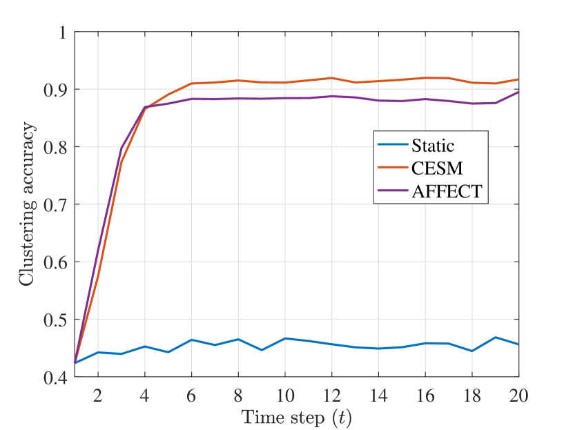
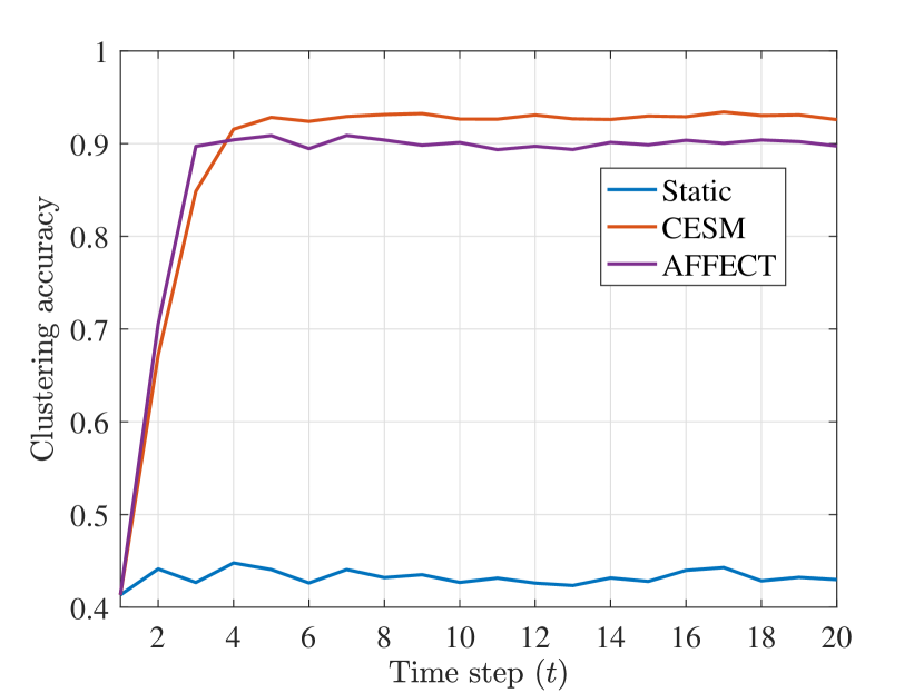
In a variety of applications including motion segmentation [10], the data points and their corresponding subspaces are characterized by rotational and transitional motions. Therefore, to simulate an underlying evolutionary process for data points lying on a union of subspaces, we consider the following scenario of rotating subspaces where we repeat each experiment for 150 trials.

At time $t=1$, we construct $n=10$ linear subspaces in ${\mathbb{R}}^{D}$, $D=10$, each with dimension $d=6$ by choosing their bases as the top $d$ left singular vectors of a random Gaussian matrix in ${\mathbb{R}}^{D\times D}$. Then, we sample $N=500$ data points, 50 from each subspace, by projecting random Gaussian vectors to the span of each subspace. Note that, in this setting, all the subspaces are distributed uniformly at random in the ambient space and all data points are uniformly distributed on the unit sphere of each subspace. According to the analysis in [32, 33, 18], this in turn implies that the subspace preserving property and the performance of representation learning methods based on BP, OMP, and AOLS is similar. However, we intentionally generate relatively low number of data points compared to the dimension of subspaces and the dimension of the ambient space; this creates a setting that is challenging for static subspace clustering algorithms. After constructing subspaces at time $t=1$, we evolve the subspaces by rotating their basis $45^{\circ}$ or $90^{\circ}$ around a random vector and project the data points ${\mathbf{X}}_{1}$ on the span of the rotated subspaces to obtain ${\mathbf{X}}_{2}$. We continue this process for $T=20$ time steps. Note that for each subspace we perform rotation around a different random vector. Otherwise, if the rotations were around the same vector, the above setting would not be an evolutionary process as the relative positions of subspaces and data points would not vary over time. For brevity, we only present results of using OMP-based learning to find the representation matrices for static and competing evolutionary subspace clustering algorithms; however, we observed similar results for representation learning methods based on BP and AOLS.

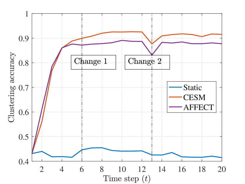
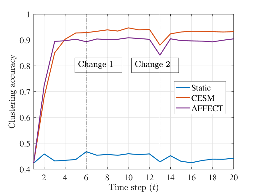
Next, we consider a related experiment where in addition to rotation, at time $t=6$ all data points generated from subspace ${\cal S}_{10}$ are absorbed by subspace ${\cal S}_{9}$. That is, at $t=6$ we project ${\mathbf{X}}_{5,{{\cal S}_{10}}}$ to the span of ${\cal S}_{9}$. At time $t=13$, these data points are separated from ${\cal S}_{9}$ and lie once again on ${\cal S}_{10}$. Hence, for $6\leq t\leq 12$ the effective number of subspaces is $n=9$ and there are 100 data points in ${\cal S}_{9}$.

The clustering accuracy results for these two experiments are illustrated in Fig. 1. For the first experiment, as seen from Fig. 1 (a) and Fig. 1 (c), the static SSC-OMP algorithm performs poorly compared to CESM and AFFECT. Since CESM and AFFECT exploit the evolutionary behavior of the data points, after a few time steps their accuracy significantly increases. We further observe that the proposed CESM framework achieves better accuracy than AFFECT; this is likely because the former exploits the self-expressiveness property of data points in the representation learning process while the latter simply combines current and prior representations to enforce the self-expressiveness property.

A comparison of the performance results in the second experiment is shown in Fig. 1 (b) and Fig. 1 (d). We observe that the performance of all evolutionary schemes suffers temporary degradations at times $t=6$ and $t=13$. The reason for this phenomenon is that the data points ${\mathbf{X}}_{6,{{\cal S}_{10}}}$ at $t=6$ are significantly different from ${\mathbf{X}}_{5,{{\cal S}_{10}}}$ at time $t=5$ due to being absorbed by ${\cal S}_{9}$ at time $t=6$ and not belonging to ${\cal S}_{10}$. Therefore, since the subspaces are nearly independent, prior representations $\{{\mathbf{c}}_{5,i}\}_{i\in{\cal S}_{10}}$ and $\{{\mathbf{c}}_{12,i}\}_{i\in{\cal S}_{10}}$ are simply not well-aligned with the sudden changes taking place at times $t=6,13$. We further note that the deterioration in clustering accuracy is more severe for AFFECT than for CESM. We also observe from the figure that the proposed evolutionary scheme is able to quickly adapt to changes. At $t=13$, the data points that were previously absorbed by ${\cal S}_{9}$ are projected back to the span of ${\cal S}_{10}$; as a result of this change, the performance of evolutionary schemes decreases. However, accuracy of the evolutionary methods recovers at $t=14$ and improves onward as they exploit the evolving property of the data. Similar to the first experiment, due to exploiting the fact that data points lie on a union of subspaces, the proposed CESM framework outperforms the AFFECT’s strategy.

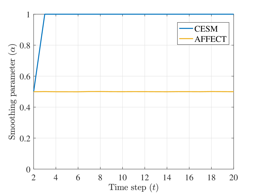
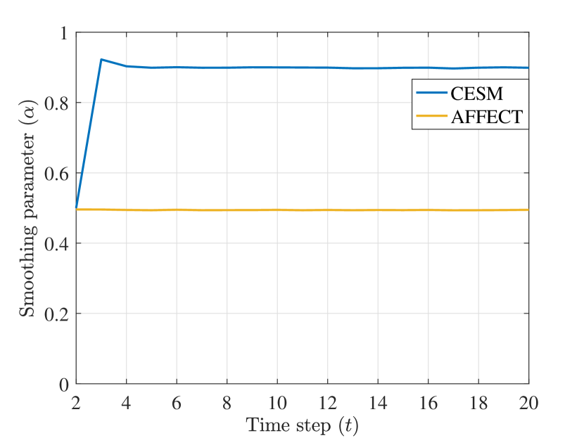
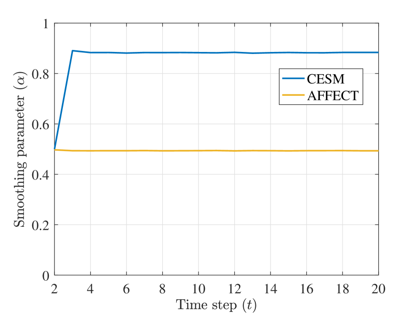
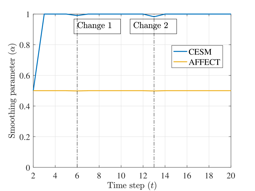
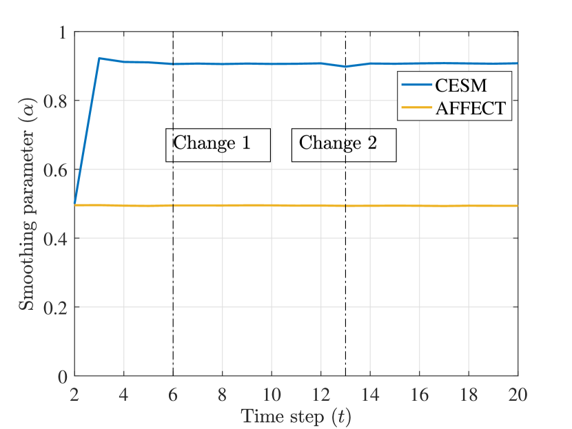
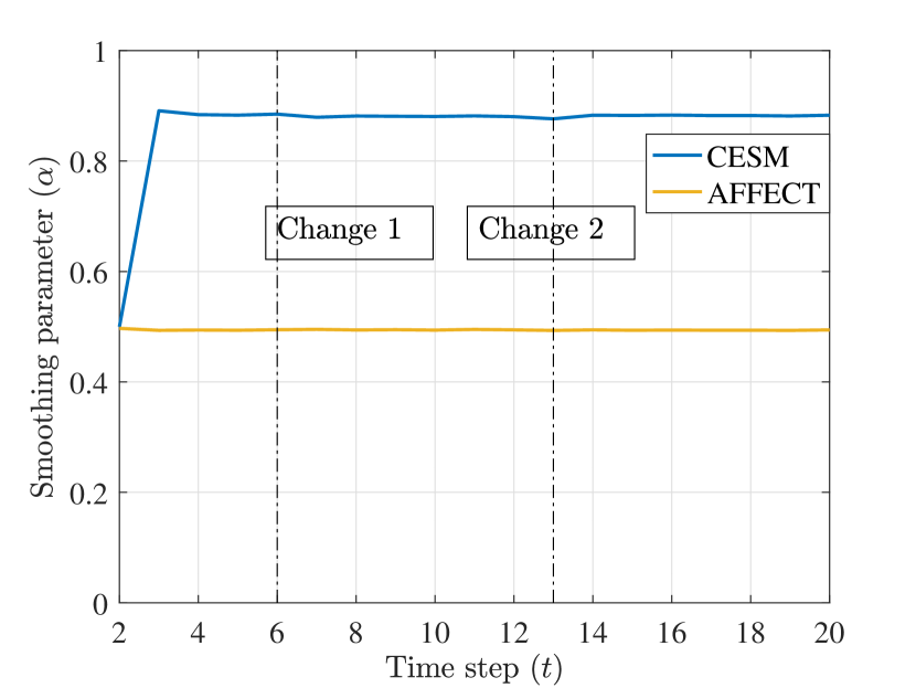
Next, we investigate the value of $\alpha$, i.e., the smoothing parameter discovered and used by CESM and AFFECT in the previously described experiments to further assess which scheme more accurately captures the evolutionary nature of the subspaces. Fig. 2 illustrates changes in the value of $\alpha$ over time, where in addition to the above two experiments we consider the scenario where subspaces are not rotating. The figure indicates that the smoothing parameter of AFFECT remains approximately $0.5$ regardless of how rapidly the subspaces evolve. Note that the smoothing parameter essentially quantifies evolutionary character of a dataset: if the data is static, we expect $\alpha=0$ or $\alpha=1$ for both CESM and AFFECT. As opposed to the AFFECT’s smoothing parameter, the value of $\alpha$ for the CESM framework quickly converges to the anticipated level; note that we initialized $\alpha$ as $0.5$. Fig. 2 (d)-(f) further suggest that the smoothing parameter of the proposed CESM framework noticeably changes at times $t=6,13$. This is a strong indication that CESM is capable of detecting subspace changes at $t=6,13$, while AFFECT fails to detect that the subspaces are rotating.

The above results suggest that the proposed framework improves performance of static subspace clustering algorithms when the data is evolving, while also being superior to state-of-the-art evolutionary clustering strategies in the considered settings. In contrast to prior schemes, the smoothing parameter of the proposed framework is meaningful and interpretable, and timely adapts to the underlying evolutionary behavior of the subspaces.

VI-B Real-time motion segmentation

Table I: Performance comparison of static and various evolutionary subspace clustering algorithms on real-time motion segmentation dataset. The best results for each row are in boldface fonts. For the CESM framework, the top results in each row correspond to the case of using a constant smoothing factor with the lowest average error while the bottom results in each row are achieved by using the proposed alternating minimization schemes to learn the smoothing parameter at each time step.

		Static				AFFECT				CESM
Learning method		error (%)	RI (%)	runtime (s)		error (%)	RI (%)	runtime (s)		error (%)	RI (%)	runtime (s)
BP		10.76	86.29	46.16		9.86	87.78	47.35		8.88 8.77	89.33 89.14	45.10 41.21
OMP		31.66	62.00	1.80		14.47	86.21	3.31		5.54 6.85	93.25 88.23	0.90 0.93
AOLS ($L=1$)		16.27	78.41	4.08		9.27	90.76	5.39		6.57 8.24	91.97 90.12	2.07 1.93
AOLS ($L=2$)		8.54	89.10	3.75		6.17	93.08	5.17		5.25 5.70	93.35 92.85	1.85 1.77
AOLS ($L=3$)		6.97	91.09	3.14		5.92	93.40	4.28		5.49 5.60	94.17 93.90	1.70 1.69

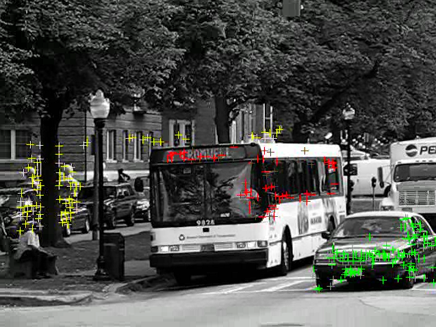
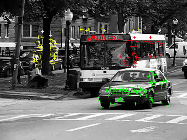
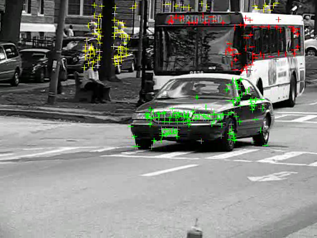
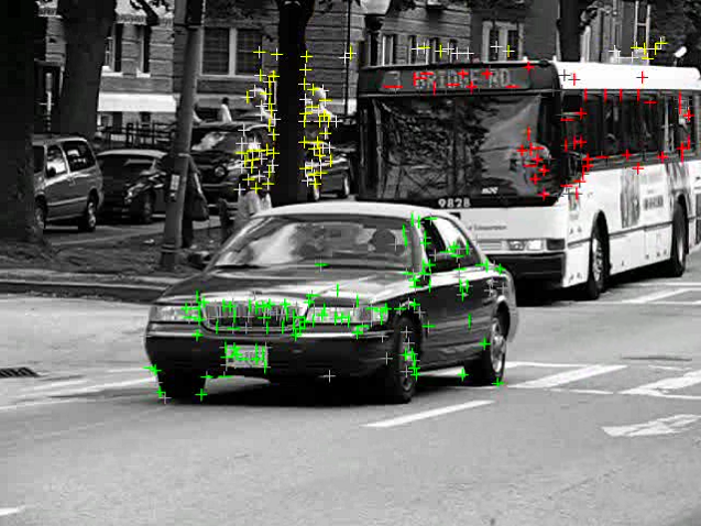
Motion segmentation is the problem of clustering a set of two dimensional trajectories extracted from a video sequence with multiple rigidly moving objects into groups; the resulting clusters correspond to different spatiotemporal regions (Fig. 3). The video sequence is often received as a stream of frames and it is desirable to perform motion segmentation in a real-time fashion [54, 55]. In the real-time setting, the $t\textsuperscript{th}$ snapshot of ${\mathbf{X}}_{t}$ (a time interval consisting of multiple video frames) is of dimension $2F_{t}\times N_{t}$, where $N_{t}$ is the number of trajectories at $t\textsuperscript{th}$ time interval, $F_{t}$ is the number of video frames received in $t\textsuperscript{th}$ time interval, $n_{t}$ is the number of rigid motions at $t\textsuperscript{th}$ time interval, and $F=\sum_{t}F_{t}$ denotes the total number of frames. Real-time motion segmentation falls within the scope of evolutionary subspace clustering since the received video sequence is naturally characterized by temporal properties; at $t\textsuperscript{th}$ time interval, the trajectories of $n_{t}$ rigid motions lie in a union of $n_{t}$ low-dimensional subspaces in ${\mathbb{R}}^{2F_{t}}$, each with the dimension of at most $d_{t}=3n_{t}$ [74].

In contrast to the real-time motion segmentation, clustering in offline settings is performed on the entire sequence, i.e., ${\mathbf{X}}={[{{\mathbf{X}}}_{1}^{\top},\dots,{{\mathbf{X}}}_{T}^{\top}]}^{\top}$. Therefore, one expects to achieve more accurate segmentation in the offline settings. However, offline motion segmentation cannot be used in scenarios where some motions vanish or new motions appear in the video, or in cases where a real-time motion segmentation solution is desired.

To benchmark the performance of the proposed CESM framework, we consider Hopkins 155 database [10] which consists of 155 video sequences with 2 or 3 motions in each video (corresponding to 2 or 3 low-dimensional subspaces). Unlike the majority of prior work that process this data set in an offline setting, we consider the following real-time scenario: each video is divided into $T$ data matrices $\{{\mathbf{X}}_{t}\}_{t=1}^{T}$ such that $F_{t}\geq 2n$ for a video with $n$ motions. Then, we apply PCA on ${\mathbf{X}}_{t}$ and take its top $D=4n$ left singular vectors as the final input to the representation learning algorithms.

We benchmark the proposed framework by comparing it to static subspace clustering and AFFECT; the former applies subspace clustering at each time step independently from the previous clustering results while the latter applies spectral clustering [14] on the weighted average of affinity matrices ${\mathbf{A}}_{t}$ and ${\mathbf{A}}_{t-1}$. The default choices for the affinity matrix in AFFECT are the negative squared Euclidean distance or its exponential form. Under these choices, AFFECT achieves a clustering error of $44.1542$ and $21.9643$ percent for the negative squared Euclidean distance or its exponential form, respectively, which as we present next is inferior even to the static subspace clustering algorithms. Hence, to fairly compare the performance of different evolutionary clustering strategies, we employ BP [58, 11, 12], OMP [60, 17, 18], and AOLS [75, 22] with $L=1,2,3$ to learn the representations for all schemes, including AFFECT.

The performance of various schemes are presented in Table I; there, the results are averaged over all sequences and all time intervals excluding the initial time interval $t=1$. The initial time interval is excluded because for a specific representation learning method (e.g., BP), the results of static subspace clustering and evolutionary schemes coincide. Note that for the proposed CESM framework, the top results in each row of Table I correspond to the case of using a constant smoothing factor with the lowest average error while the bottom results in each row are achieved by using the proposed alternating minimization schemes to learn the best smoothing parameter for each time interval.

As we can see from the table, static subspace clustering has higher clustering errors than their evolutionary counterparts; this is due to not incorporating any knowledge about the representations of the data points at other times. Furthermore, the proposed CESM framework is superior to AFFECT in terms of clustering error for all the representation learning methods. In addition, the proposed CESM framework achieves lower running time than static and AFFECT strategies, especially for the case of using OMP and AOLS as the representation learning methods. This supports the observation that CESM promotes sparser ${\mathbf{U}}_{t}$ by leveraging ${\mathbf{C}}_{t-1}$ in the process of learning ${\mathbf{C}}_{t}$ which in turn leads to faster convergence of OMP and AOLS. Similar to what we observed on synthetic datasets, the smoothing parameter of AFFECT (with both the default choices for the affinity matrix and the SSC-based affinity learning methods) was approximately $0.5$ for all sequences and thus unable to capture evolutionary structure of the subspaces in a meaningful and interpretable manner.

VI-C Ocean water mass clustering

(a) static

(b) AFFECT

(c) CESM

Fig. 4: Clustering results of four different types of water masses at 1000 dbar near the coast of south Africa (colored with blue). using static and various evolutionary subspace clustering schemes employing AOLS-based representation learning strategy with $L=3$. The static subspace clustering scheme and AFFECT fail to keep track of the orange water mass at time $t=6$ and $t=4$, respectively. However, our proposed CESM framework detects homogeneous water masses across all time steps.

Table II: Average salinity and temperature of four different types of water masses at 1000 dbar near the coast of south Africa identified by CESM framework employing AOLS-based representation learning strategy with $L=3$ at different time steps. The results in top, middle and bottom for each cluster correspond to $t=2,4,6$, respectively.

water mass		salinity level		temperature (∘C)
orange		34.4554 34.3564 34.5008		3.4971 3.6164 3.2141
green		34.3452 34.6693 34.3640		3.5849 1.9910 3.6482
yellow		34.6603 34.4974 34.6680		2.0177 6.4445 2.0914
purple		34.4998 34.4649 34.4997		6.3313 3.4162 6.5522

Ocean temperature and salinity has been tracked by Argo ocean observatory system comprising more than 3000 floats which provide 100,000 plus temperature and salinity profiles each year. These floats cycle between the ocean surface and 2000m depth every 10 days, taking salinity and temperature measurements at varying depths. A water mass is characterized as a body of water with a common formation and homogeneous features, such as salinity and temperature. Study of water masses can provide insight into climate change, seasonal climatological variations, ocean biogeochemistry, and ocean circulation and its effect on transport of oxygen and organisms, which in turn affects the biological diversity of an area.

To illustrate the abilities of evolutionary subspace clustering in modeling various real-world problems, including those outside the computer vision community, we analyze the global gridded dataset produced via the Barnes method that was collected and made freely available by the international Argo program. This dataset contains monthly averages (since January 2004) of ocean temperature and salinity with 1 degree resolution worldwide [76, 77].

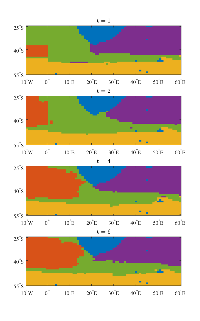
In order to identify homogeneous water masses, we apply static and various evolutionary subspace clustering schemes, using AOLS-based representation learning method with $L=3$ on the temperature and salinity data at the location near the coast of South Africa where the Indian Ocean meets the South Atlantic (specifically, the area located at latitudes 25^∘ S to 55^∘ S and longitudes 10^∘ W to 60^∘ E).

According to prior studies in [78, 79, 80], there are three well-known and strong mater masses in this area: (1) Agulhas currents, (2) the Antarctic intermediate water (AAIW), and (3) the circumpolar deep water mass. Therefore, following the discussion in [78] we set the number of clusters to $n=4$ to further account for other water masses in the area.

The area described above accounts for $N=1921$ evolving data points, each containing the monthly salinity and temperature from April to September for two years acquired starting in the year 2004 and 2005 ($t=1$) until year 2014 and 2015 ($t=6$). Temperature and salinity were normalized by subtracting the mean and dividing by the standard deviation of the entire time frame of interest. This procedure results in $24\times N$ data matrices $\{{\mathbf{X}}_{t}\}_{t=1}^{6}$ which are then used as inputs to the evolutionary subspace clustering algorithms. As stated in Section V, we employ the Hungarian method [62] to match the clustering solution at each time to the previous result.

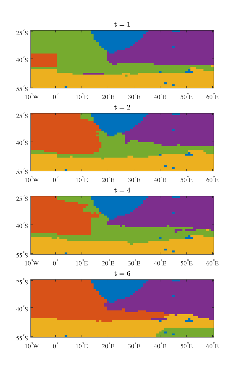
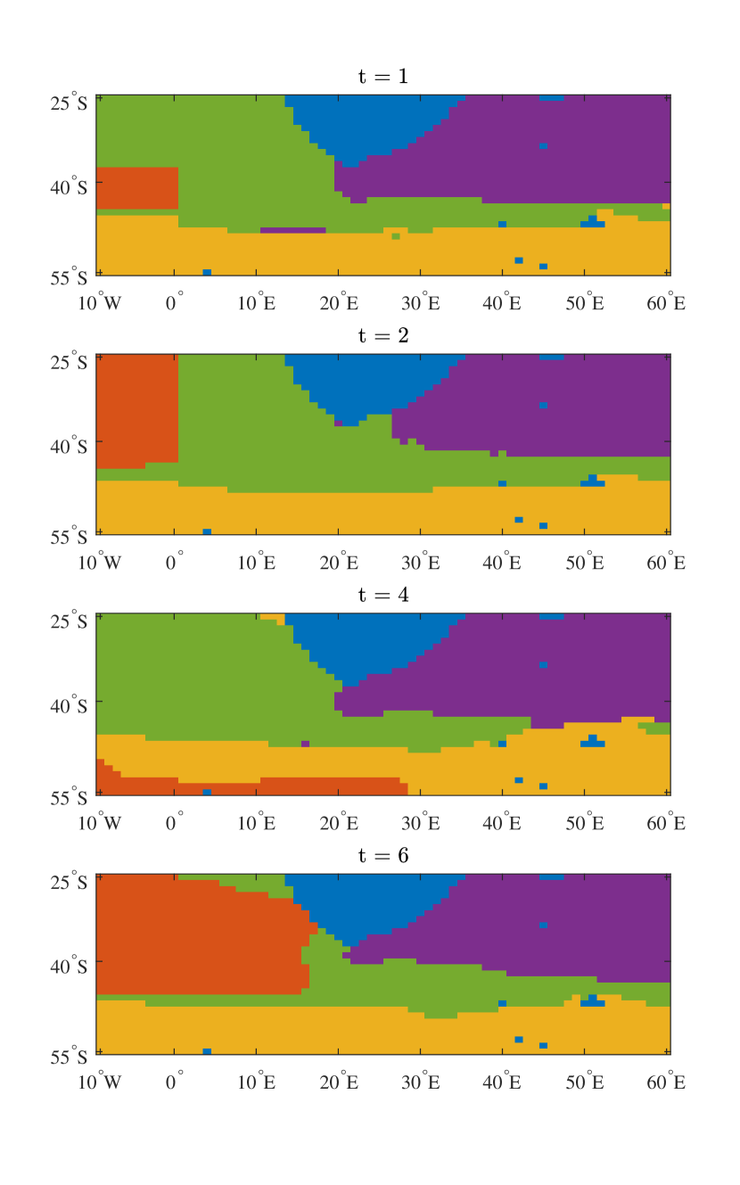
The identified water masses by static, AFFECT, and CESM schemes using AOLS with $L=3$ as the representation learning method are illustrated in Fig. 4 for $t=1,2,4,6$. The area colored with blue corresponds to the coast of south Africa and other islands in the target location. As we can see from the figure, all schemes are able to identify homogeneous water masses. However, the static subspace clustering and AFFECT schemes fail to properly detect the temporal changes in the formation of the green and orange water masses. In particular, the formation of the orange cluster evolves, as captured by the clustering results of the CESM framework. Since the CESM framework accounts for the underlying temporal behavior in the representation learning process and are able to infer appropriate smoothing factors, they are able to accurately keep track of the orange and green clusters across different time steps. Note that similarly to the results on synthetic and real-time motion segmentation datasets, the smoothing parameter of AFFECT was approximately $0.5$. In addition, compared to AFFECT, CESM framework is capable of a faster adaptation to the changes in the formation of the orange water mass from $t=1$ to $t=2$.

The temperature and salinity averages for the water masses clustered by the CESM framework are shown in Table II where the results in top, middle and bottom for each cluster correspond to $t=2,4,6$, respectively. A combination of these values, the geographic location of the clusters, and prior studies in [78, 79] suggest that the purple, orange, and yellow clusters corresponds to Agulhas currents, AAIW, and the circumpolar deep water masses, respectively.

VII Conclusion

In this paper, we studied the problem of evolutionary subspace clustering that is concerned with organizing a collection of data points that lie on a union of low-dimensional temporally evolving subspaces. Unlike existing evolutionary clustering frameworks, the evolving data in evolutionary subspace clustering is assumed to be self-expressive, i.e., each data point can be represented by a linear combination of other data points in the set. By relying on the self-expressiveness property, we proposed a non-convex optimization framework that enables learning parsimonious representations of data points at each time step while taking into account representations from the preceding time step. The proposed framework utilizes a convex evolutionary self-expressive model (CESM) to establish a relation between current and previous representations. Finding parameters of CESM leads to a non-convex optimization problem; we developed schemes that rely on alternating minimization to solve it approximately and to adaptively tune a smoothing parameter that is reflective of the rate of evolution, i.e., indicates to what extent the representations in consecutive time steps are similar to each other. Our extensive studies on both synthetic and real-world datasets illustrate that the proposed CESM framework outperforms state-of-the-art static subspace clustering and evolutionary clustering schemes in majority of scenarios in terms of both accuracy and running time. Furthermore, the smoothing parameter learned by the proposed framework is interpretable and reflective of the “memory” of data representation in consecutive time steps.

As part of the future work, it would be of interest to extend the CESM framework to other subspace clustering algorithms, including the schemes that rely on finding low rank representations of data points. It is also valuable to exploit the theoretical foundation of subspace clustering to analyze the performance of the proposed frameworks, e.g., in the setting of rotating random subspaces that we considered in this paper. Finally, it would be of interest to develop more complex models for the evolutionary subspace clustering problem, e.g., by using neural networks as the parametric function or a matrix of smoothing parameters in place of the proposed convex evolutionary self-expressive model.

References

- [1] A. Y. Yang, J. Wright, Y. Ma, and S. S. Sastry, “Unsupervised segmentation of natural images via lossy data compression,” Computer Vision and Image Understanding, vol. 110, no. 2, pp. 212–225, May 2008.
- [2] R. Vidal, R. Tron, and R. Hartley, “Multiframe motion segmentation with missing data using PowerFactorization and GPCA,” Int. Journal of Computer Vision, vol. 79, no. 1, pp. 85–105, Aug. 2008.
- [3] J. Ho, M.-H. Yang, J. Lim, K.-C. Lee, and D. Kriegman, “Clustering appearances of objects under varying illumination conditions,” in Conf. Computer Vision and Pattern Recognition (CVPR), vol. 1, pp. I–I, IEEE, 2003.
- [4] W. Hong, J. Wright, K. Huang, and Y. Ma, “Multiscale hybrid linear models for lossy image representation,” IEEE Trans. Image Process., vol. 15, no. 12, pp. 3655–3671, Dec. 2006.
- [5] H. Xu, C. Caramanis, and S. Sanghavi, “Robust PCA via outlier pursuit,” in Advances in Neural Information Processing Systems (NIPS), pp. 2496–2504, 2010.
- [6] E. J. Candès, X. Li, Y. Ma, and J. Wright, “Robust principal component analysis?,” Journal of the ACM, vol. 58, no. 3, p. 11, May 2011.
- [7] B. Yang, “Projection approximation subspace tracking,” IEEE Trans. Signal Process., vol. 43, no. 1, pp. 95–107, Jan. 1995.
- [8] M. Rahmani and G. K. Atia, “High dimensional low rank plus sparse matrix decomposition,” IEEE Trans. Signal Process., vol. 65, no. 8, pp. 2004–2019, Apr. 2017.
- [9] M. Rahmani and G. K. Atia, “Randomized robust subspace recovery and outlier detection for high dimensional data matrices,” IEEE Trans. Signal Process., vol. 65, no. 6, pp. 1580–1594, Mar. 2017.
- [10] R. Tron and R. Vidal, “A benchmark for the comparison of 3-D motion segmentation algorithms,” in Conf. Computer Vision and Pattern Recognition (CVPR), pp. 1–8, IEEE, 2007.
- [11] E. Elhamifar and R. Vidal, “Sparse subspace clustering,” in Conf. Computer Vision and Pattern Recognition (CVPR), pp. 2790–2797, IEEE, 2009.
- [12] E. Elhamifar and R. Vidal, “Sparse subspace clustering: Algorithm, theory, and applications,” IEEE Trans. Pattern Anal. Mach. Intell., vol. 35, no. 11, pp. 2765–2781, Nov. 2013.
- [13] R. Vidal, “Subspace clustering,” IEEE Signal Processing Magazine, vol. 28, no. 2, pp. 52–68, Mar. 2011.
- [14] A. Y. Ng, M. I. Jordan, Y. Weiss, et al., “On spectral clustering: Analysis and an algorithm,” in the Advances in Neural Information Processing Systems (NIPS), vol. 14, pp. 849–856, 2001.
- [15] S.-J. Kim, K. Koh, M. Lustig, S. Boyd, and D. Gorinevsky, “An interior-point method for large-scale -regularized least squares,” IEEE Journal of Selected Topics in Signal Processing, vol. 1, no. 4, pp. 606–617, Dec. 2007.
- [16] S. Boyd, N. Parikh, E. Chu, B. Peleato, and J. Eckstein, “Distributed optimization and statistical learning via the alternating direction method of multipliers,” Foundations and Trends® in Machine Learning, vol. 3, no. 1, pp. 1–122, Jan. 2011.
- [17] E. L. Dyer, A. C. Sankaranarayanan, and R. G. Baraniuk, “Greedy feature selection for subspace clustering,” The Journal of Machine Learning Research, vol. 14, no. 1, pp. 2487–2517, Sep. 2013.
- [18] C. You, D. Robinson, and R. Vidal, “Scalable sparse subspace clustering by orthogonal matching pursuit,” in Conf. Computer Vision and Pattern Recognition (CVPR), pp. 3918–3927, IEEE, 2016.
- [19] M. Tschannen and H. Bölcskei, “Noisy subspace clustering via matching pursuits,” arXiv preprint arXiv:1612.03450, Dec. 2016.
- [20] Y. Chen, G. Li, and Y. Gu, “Active orthogonal matching pursuit for sparse subspace clustering,” IEEE Signal Processing Letters, vol. 25, no. 2, pp. 164–168, Feb. 2018.
- [21] D. Park, C. Caramanis, and S. Sanghavi, “Greedy subspace clustering,” in Advances in Neural Information Processing Systems (NIPS), pp. 2753–2761, 2014.
- [22] A. Hashemi and H. Vikalo, “Accelerated sparse subspace clustering,” arXiv preprint arXiv:1711.00126, Oct. 2017.
- [23] M. Rahmani and G. K. Atia, “Innovation pursuit: A new approach to subspace clustering,” IEEE Trans. Signal Process., vol. 65, pp. 6276–6291, Dec. 2017.
- [24] C.-Y. Lu, H. Min, Z.-Q. Zhao, L. Zhu, D.-S. Huang, and S. Yan, “Robust and efficient subspace segmentation via least squares regression,” in European Conf. computer vision (ECCV), pp. 347–360, Springer, 2012.
- [25] G. Liu, Z. Lin, S. Yan, J. Sun, Y. Yu, and Y. Ma, “Robust recovery of subspace structures by low-rank representation,” IEEE Trans. Pattern Anal. Mach. Intell., vol. 35, no. 1, pp. 171–184, Jan. 2013.
- [26] P. Favaro, R. Vidal, and A. Ravichandran, “A closed form solution to robust subspace estimation and clustering,” in the IEEE Conf. Computer Vision and Pattern Recognition (CVPR), pp. 1801–1807, IEEE, 2011.
- [27] R. Vidal and P. Favaro, “Low rank subspace clustering (LRSC),” Pattern Recognition Letters, vol. 43, pp. 47–61, Jul. 2014.
- [28] J. Feng, Z. Lin, H. Xu, and S. Yan, “Robust subspace segmentation with block-diagonal prior,” in Conf. on Computer Vision and Pattern Recognition (CVPR), pp. 3818–3825, 2014.
- [29] H. Gao, F. Nie, X. Li, and H. Huang, “Multi-view subspace clustering,” in Conf. on Computer Vision and Pattern Recognition (CVPR), pp. 4238–4246, 2015.
- [30] F. Nie and H. Huang, “Subspace clustering via new low-rank model with discrete group structure constraint,” in Int. Joint. Conf. Artificial Intell. (IJCAI), pp. 1874–1880, 2016.
- [31] R. Heckel and H. Bölcskei, “Robust subspace clustering via thresholding,” IEEE Trans. Inf. Theory, vol. 61, no. 11, pp. 6320–6342, Nov. 2015.
- [32] M. Soltanolkotabi and E. J. Candes, “A geometric analysis of subspace clustering with outliers,” The Annals of Statistics, pp. 2195–2238, Aug. 2012.
- [33] M. Soltanolkotabi, E. Elhamifar, and E. J. Candes, “Robust subspace clustering,” The Annals of Statistics, vol. 42, no. 2, pp. 669–699, Apr. 2014.
- [34] C.-G. Li, C. You, and R. Vidal, “Structured sparse subspace clustering: A joint affinity learning and subspace clustering framework,” IEEE Trans. Image Process., vol. 26, no. 6, pp. 2988–3001, Jun. 2017.
- [35] E. Elhamifar, “High-rank matrix completion and clustering under self-expressive models,” in Advances in Neural Information Processing Systems (NIPS), pp. 73–81, 2016.
- [36] C.-G. Li and R. Vidal, “A structured sparse plus structured low-rank framework for subspace clustering and completion,” IEEE Trans. Signal Process., vol. 64, no. 24, pp. 6557–6570, Dec. 2016.
- [37] J. Fan and T. W. Chow, “Sparse subspace clustering for data with missing entries and high-rank matrix completion,” Neural Networks, vol. 93, pp. 36–44, Sep. 2017.
- [38] Z. Charles, A. Jalali, and R. Willett, “Subspace clustering with missing and corrupted data,” arXiv preprint arXiv:1707.02461, Jan. 2018.
- [39] M. C. Tsakiris and R. Vidal, “Theoretical analysis of sparse subspace clustering with missing entries,” arXiv preprint arXiv:1801.00393, Feb. 2018.
- [40] J. Shen, P. Li, and H. Xu, “Online low-rank subspace clustering by basis dictionary pursuit,” in Int. Conf. Machine Learning (ICML), pp. 622–631, 2016.
- [41] S. Li, K. Li, and Y. Fu, “Temporal subspace clustering for human motion segmentation,” in Int. Conf. Computer Vision (ICCV), pp. 4453–4461, IEEE, 2015.
- [42] D. Chakrabarti, R. Kumar, and A. Tomkins, “Evolutionary clustering,” in Int. Conf. Knowledge Discovery and Data Mining (SIGKDD), pp. 554–560, ACM, 2006.
- [43] K. S. Xu, M. Kliger, and A. O. Hero III, “Adaptive evolutionary clustering,” Data Mining and Knowledge Discovery, vol. 28, no. 2, pp. 304–336, Mar. 2014.
- [44] F. Folino and C. Pizzuti, “An evolutionary multiobjective approach for community discovery in dynamic networks,” IEEE Transactions on Knowledge and Data Engineering, vol. 26, no. 8, pp. 1838–1852, Aug. 2014.
- [45] N. M. Arzeno and H. Vikalo, “Evolutionary affinity propagation,” in Int. Conf. Acoustics, Speech and Signal Processing (ICASSP), pp. 2681–2685, IEEE, 2017.
- [46] N. Czink, R. Tian, S. Wyne, F. Tufvesson, J.-P. Nuutinen, J. Ylitalo, E. Bonek, and A. F. Molisch, “Tracking time-variant cluster parameters in MIMO channel measurements,” in Int. Conf. Communications and Networking in China (CHINACOM), pp. 1147–1151, IEEE, 2007.
- [47] S. Günnemann, H. Kremer, C. Laufkötter, and T. Seidl, “Tracing evolving subspace clusters in temporal climate data,” Data Mining and Knowledge Discovery, vol. 24, no. 2, pp. 387–410, Mar. 2012.
- [48] A. Ahmed and E. Xing, “Dynamic non-parametric mixture models and the recurrent Chinese restaurant process: With applications to evolutionary clustering,” in Int. Conf. Data Mining (SDM), pp. 219–230, SIAM, 2008.
- [49] T. Xu, Z. Zhang, S. Y. Philip, and B. Long, “Evolutionary clustering by hierarchical Dirichlet process with hidden Markov state,” in Int. Conf. Data Mining (ICDM), pp. 658–667, IEEE, 2008.
- [50] A. Ahmed and E. P. Xing, “Timeline: A dynamic hierarchical Dirichlet process model for recovering birth/death and evolution of topics in text stream,” arXiv preprint arXiv:1203.3463, Mar. 2012.
- [51] Y. Chi, X. Song, D. Zhou, K. Hino, and B. L. Tseng, “Evolutionary spectral clustering by incorporating temporal smoothness,” in Int. Conf. Knowledge Discovery and Data Mining (SIGKDD), pp. 153–162, ACM, 2007.
- [52] Y. Chi, X. Song, D. Zhou, K. Hino, and B. L. Tseng, “On evolutionary spectral clustering,” ACM Transactions on Knowledge Discovery from Data, vol. 3, no. 4, p. 17, Nov. 2009.
- [53] J. Rosswog and K. Ghose, “Detecting and tracking spatio-temporal clusters with adaptive history filtering,” in Int. Conf. Data Mining Workshops (ICDMW), pp. 448–457, IEEE, 2008.
- [54] S. M. Smith and J. M. Brady, “ASSET-2: Real-time motion segmentation and shape tracking,” IEEE Trans. Pattern Anal. Mach. Intell., vol. 17, no. 8, pp. 814–820, Aug. 1995.
- [55] R. T. Collins, Y. Liu, and M. Leordeanu, “Online selection of discriminative tracking features,” IEEE Trans. Pattern Anal. Mach. Intell., vol. 27, no. 10, pp. 1631–1643, Aug. 2005.
- [56] J. Kiefer, “Sequential minimax search for a maximum,” the American Mathematical Society, vol. 4, no. 3, pp. 502–506, Sep. 1953.
- [57] D. L. Donoho, “Compressed sensing,” IEEE Trans. Inf. Theory, vol. 52, no. 4, pp. 1289–1306, Apr. 2006.
- [58] S. S. Chen, D. L. Donoho, and M. A. Saunders, “Atomic decomposition by basis pursuit,” SIAM review, vol. 43, no. 1, pp. 129–159, Feb. 2001.
- [59] R. Tibshirani, “Regression shrinkage and selection via the LASSO,” Journal of the Royal Statistical Society. Series B (Methodological), pp. 267–288, Jan. 1996.
- [60] Y. C. Pati, R. Rezaiifar, and P. S. Krishnaprasad, “Orthogonal matching pursuit: Recursive function approximation with applications to wavelet decomposition,” in Asilomar Conf. Signals, Syst. and Computers, pp. 40–44, IEEE, 1993.
- [61] S. Chen, S. A. Billings, and W. Luo, “Orthogonal least squares methods and their application to non-linear system identification,” Int. Journal of Control, vol. 50, no. 5, pp. 1873–1896, Nov. 1989.
- [62] H. W. Kuhn, “The Hungarian method for the assignment problem,” Naval Research Logistics, vol. 2, no. 1-2, pp. 83–97, Mar. 1955.
- [63] D. Greene, D. Doyle, and P. Cunningham, “Tracking the evolution of communities in dynamic social networks,” in Int. Conf. Advances in Social Networks Analysis and Mining (ASONAM), pp. 176–183, IEEE, 2010.
- [64] P. Bródka, S. Saganowski, and P. Kazienko, “GED: The method for group evolution discovery in social networks,” Social Network Analysis and Mining, vol. 3, no. 1, pp. 1–14, Mar. 2013.
- [65] J. Yang and Y. Zhang, “Alternating direction algorithms for -problems in compressive sensing,” SIAM Journal on Scientific Computing, vol. 33, no. 1, pp. 250–278, Feb. 2011.
- [66] J. Yang and X. Yuan, “Linearized augmented lagrangian and alternating direction methods for nuclear norm minimization,” Mathematics of Computation, vol. 82, no. 281, pp. 301–329, Jan. 2013.
- [67] T. Goldstein, B. O’Donoghue, S. Setzer, and R. Baraniuk, “Fast alternating direction optimization methods,” SIAM Journal on Imaging Sciences, vol. 7, no. 3, pp. 1588–1623, Aug. 2014.
- [68] Z. Lin, R. Liu, and H. Li, “Linearized alternating direction method with parallel splitting and adaptive penalty for separable convex programs in machine learning,” Machine Learning, vol. 99, no. 2, pp. 287–325, May 2015.
- [69] B. Mirzasoleiman, A. Badanidiyuru, A. Karbasi, J. Vondrak, and A. Krause, “Lazier than lazy greedy,” in Conf. Artificial Intell., AAAI, 2015.
- [70] G. L. Nemhauser, L. A. Wolsey, and M. L. Fisher, “An analysis of approximations for maximizing submodular set functions I,” Mathematical Programming, vol. 14, no. 1, pp. 265–294, Dec. 1978.
- [71] A. Das and D. Kempe, “Submodular meets spectral: Greedy algorithms for subset selection, sparse approximation and dictionary selection,” in Int. Conf. Machine Learning, pp. 1057–1064, 2011.
- [72] A. Hashemi, M. Ghasemi, H. Vikalo, and U. Topcu, “A randomized greedy algorithm for near-optimal sensor scheduling in large-scale sensor networks,” in American Control Conference (ACC), 2018.
- [73] A. Hashemi and H. Vikalo, “Accelerated orthogonal least-squares for large-scale sparse reconstruction,” Digital Signal Process., vol. 82, pp. 91–105, Nov. 2018.
- [74] C. Tomasi and T. Kanade, “Shape and motion from image streams under orthography: A factorization method,” Int. Journal of Computer Vision, vol. 9, no. 2, pp. 137–154, Nov. 1992.
- [75] A. Hashemi and H. Vikalo, “Sparse linear regression via generalized orthogonal least-squares,” in Global Conf. Signal and Information Processing (GlobalSIP), pp. 1305–1309, IEEE, Dec. 2016.
- [76] D. Roemmich and J. Gilson, “The 2004–2008 mean and annual cycle of temperature, salinity, and steric height in the global ocean from the Argo program,” Progress in Oceanography, vol. 82, no. 2, pp. 81–100, Aug. 2009.
- [77] H. Li, F. Xu, W. Zhou, D. Wang, J. S. Wright, Z. Liu, and Y. Lin, “Development of a global gridded Argo data set with Barnes successive corrections,” Journal of Geophysical Research: Oceans, vol. 122, no. 2, pp. 866–889, Jan. 2017.
- [78] N. M. Arzeno-González, Outcome prediction and structure discovery in healthcare data. PhD thesis, 2016.
- [79] G. L. Pickard and W. J. Emery, Descriptive physical oceanography: An introduction. Elsevier, 2016.
- [80] N. M. Arzeno-González and H. Vikalo, “Evolutionary clustering via message passing,” Submitted, 2018.