Learning stable and predictive structures in kinetic systems: Benefits of a causal approach

Abstract

Learning kinetic systems from data is one of the core challenges in many fields. Identifying stable models is essential for the generalization capabilities of data-driven inference. We introduce a computationally efficient framework, called CausalKinetiX, that identifies structure from discrete time, noisy observations, generated from heterogeneous experiments. The algorithm assumes the existence of an underlying, invariant kinetic model, a key criterion for reproducible research. Results on both simulated and real-world examples suggest that learning the structure of kinetic systems benefits from a causal perspective. The identified variables and models allow for a concise description of the dynamics across multiple experimental settings and can be used for prediction in unseen experiments. We observe significant improvements compared to well established approaches focusing solely on predictive performance, especially for out-of-sample generalization.

Introduction

Quantitative models of kinetic systems have become a cornerstone of the modern natural sciences and are universally used in scientific fields as diverse as physics, neuroscience, genetics, bioprocessing, robotics or economics Friston et al. (2003); Chen et al. (1999); Ogunnaike and Ray (1994); Murray (2017); Zhang (2005). In systems biology, mechanistic models based on differential equations, although not yet standard, are being increasingly used, for example, as biomarkers to predict patient outcomes Fey et al. (2015), to improve predicting ligand dependent tumors Hass et al. (2017) or for developing mechanism-based cancer therapeutics Arteaga and Engelman (2014). While the advantages of a mechanistic modeling approach are by now well established, deriving such models from hand is a difficult and labour intensive manual effort. With new data acquisition technologies Ren et al. (2003); Regev et al. (2017); Rozman et al. (2018) learning kinetic systems from data has become a core challenge.

Existing data driven approaches infer the parameters of ordinary differential equations by considering the goodness-of-fit of the integrated system as a loss function Bard (1974); Benson (1979). To infer the structure of such models, standard model selection techniques and sparsity enforcing regularizations can be used. When evaluating the loss function or perfoming an optimization step, these methods rely on numerically integrating the kinetic system. There are various versions, and here we concentrate on the highly optimized Matlab implementation data2dynamics Raue et al. (2015). It can be considered as a state-of-the-art implementation for directly performing an integration in each evaluation of the loss function. However, even with highly optimized integration procedures, the computational cost of existing methods is high and depending on the model class, these procedures can be infeasible. Moreover, existing data driven approaches, not only those using numerical integration, infer the structure of ordinary differential equations from a single environment, possibly containing data pooled from several experiments, and focus solely on predictive performance. Such predictive based procedures have difficulties in capturing the underlying causal mechanism and as a result, they may not predict well the outcome of experiments that are different from the ones used for fitting the model.

Here, we propose an approach to model the dynamics of a single target variable rather than the full system. The resulting computational gain allows our method to scale to systems with many variables. By efficiently optimizing a non-invariance score our algorithm consistently identifies causal kinetic models that are invariant across heterogeneous experiments. In situations, where there is not sufficient heterogeneity to guarantee identification of a single causal model, the proposed variable ranking may still be used to generate causal hypotheses and candidates suitable for further investigation. We demonstrate that our novel framework is robust against model misspecification and the existence of hidden variables. The proposed algorithm is implemented and available as an open source R-package. The results on both simulated and real-world examples suggest that learning the structure of kinetic systems benefits from taking into account invariance, rather than focusing solely on predictive performance. This finding aligns well with a recent debate in data science proposing to move away from predictability as the sole principle of inference (Schölkopf et al., 2012; Yu, 2013; Peters et al., 2016; Bareinboim and Pearl, 2016; Meinshausen et al., 2016; Shiffrin, 2016; Yu and Kumbier, 2019).

Results

Predictive models versus causal models.

Established methods mostly focus on predictability when inferring biological structure from data by selecting models. This learning principle, however, does not necessarily yield models that generalize well to unseen experiments, since purely predictive models remain agnostic with respect to changing environments or experimental settings. Causal models Pearl (2009); Imbens and Rubin (2015) explicitly model such changes by the concept of interventions. The principle of autonomy or modularity of a system Haavelmo (1944); Aldrich (1989) states that the mechanisms which are not intervened on, remain invariant (or stable). This is why causal models are expected to work more reliably when predicting under distributional shifts Pearl and Mackenzie (2018); Peters et al. (2017); Oates et al. (2014).

Causality through stability.

In most practical applications the causal structure is unknown, but it may still be possible to infer the direct causes of a target variable $Y$, say, if the system is observed under different, possibly unspecified experimental settings. For non-dynamical data, this can be achieved by searching for models that are stable across all experimental conditions, i.e., the parameter estimates are similar. Covariates that are contained in all stable models, i.e., in their intersection, can be proven to be causal predictors for $Y$ (Peters et al., 2016; Eaton and Murphy, 2007). The intersection of stable models, however, is not necessarily a good predictive model. In this work, we propose a method for dynamical systems that combines stability with predictability, we show that the inferred models generalize to unseen experiments and we formalize its relation to causality (Methods).

CausalKinetiX: combining stability and predictability.

The observed data consist of a target variable $Y$ and covariates $X$ measured at several time points across different experimental setups and is assumed to be corrupted with observational noise, Figure 1 (top). Our proposed method, CausalKinetiX, exploits the assumption that the model governing the dynamics of $Y$ remains invariant over the different experiments. We assume there is a subset $S^{*}$ of covariates, s.t. for all $n$ repetitions, $\frac{d}{dt}Y_{t}$ depends on the covariates in the same way, i.e.,

$$\tfrac{d}{dt}Y^{(i)}_{t}=f\big{(}{X}^{S^{*},(i)}_{t}\big{)},\,\text{ for all }i=1,\ldots,n.$$ (1)

The covariates are allowed to change arbitrarily across different repetitions $i$. Instead of only fitting based on predictive power, CausalKinetiX explicitly measures and takes into account violations of the invariance in [1]. Figure 1 depicts the method’s full workflow.

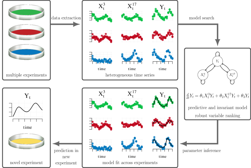
Figure 1: The framework of CausalKinetiX: the data for a target variables $Y$ and predictors $X$ come from different experiments; we rank models according to their ability to fit the target well in all experiments; the top ranked model is then fit to the data; it allows to predict the target in an unseen experiment.

It ranks a collection of candidate models $\mathcal{M}=\{M_{1},\dots,M_{m}\}$ for the target variable (Methods) based both on their predictive performance and whether the invariance in [1] is satisfied. For a single model, e.g., $\frac{d}{dt}Y_{t}^{(i)}=\theta X^{8,(i)}_{t}$, and noisy realizations $\widetilde{Y}_{t_{1}}^{(i)},\ldots,\widetilde{Y}_{t_{L}}^{(i)}$, we propose to compare the two data fits illustrated in Figure 2.

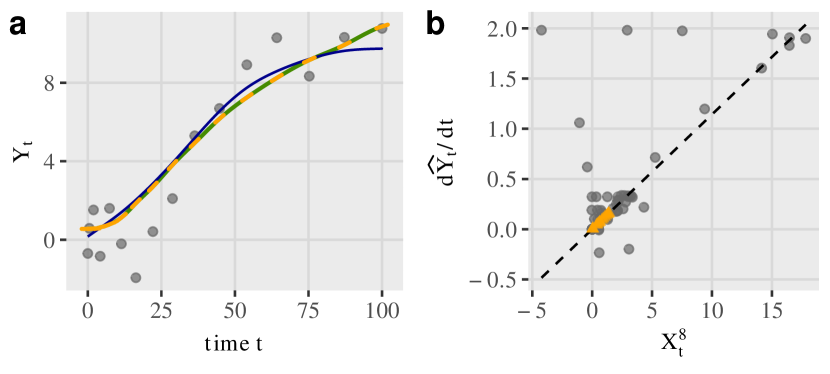
Figure 2: CausalKinetiX assigns a score to each model that trades-off predictability and invariance. Here, we consider the model $dY_{t}/dt=\theta X^{8}_{t}$. a, For each realization, two data fits are considered. An entirely data-driven nonlinear smoother (Data Fit A, blue) is compared against a model based fit (Data Fit B, green) with constraints on the derivatives (orange lines). b, The derivative constraints are obtained from all other experiments: they correspond to fitted values (orange triangles) in a regression of the estimated derivatives on the predictors.

Data Fit A calculates a smoothing spline to the data using all realization from the same experiment, see [10]. This fit only serves as a baseline for comparison: it does not incorporate the form of the underlying kinetic model, but is entirely data-driven. To obtain Data Fit B, we fit the considered model, $\frac{d}{dt}Y_{t}=\theta X^{8}_{t}$, on the data from all other experiments (explicitly leaving out the current experiment) by regressing estimated derivatives on the predictor variables. In this example, the model is linear in its parameters, and it therefore suffices to use linear regression. Data fit B fits a smoothing spline to the same data, subject to the constraint that its derivatives coincide with the fitted values from the regression inferred solely based on the other experiments, see [12]. Data fits A and B are compared by considering the goodness-of-fit for each realization $i=1,\ldots,n$. More specifically, each model $M\in\mathcal{M}$ obtains, similar in spirit to Lim and Yu (2016), the non-invariance score

$$T(M)\coloneqq\frac{1}{n}\sum_{i=1}^{n}\left[{\operatorname{RSS}_{B}^{(i)}-\operatorname{RSS}_{A}^{(i)}}\right]/\left[\operatorname{RSS}_{A}^{(i)}\right],$$

where $\operatorname{RSS}_{*}^{(i)}\coloneqq\frac{1}{L}\sum_{\ell=1}^{L}(\hat{y}^{(i)}_{*}(t_{\ell})-\widetilde{Y}^{(i)}_{t_{\ell}})^{2}$ is the residual sum of squares based on the respective data fits $\hat{y}_{A}^{(i)}$ and $\hat{y}_{B}^{(i)}$. Due to the additional constraints, $\operatorname{RSS}_{B}$ is always larger than $\operatorname{RSS}_{A}$.

The score is large either if the considered model does not fit the data well or if the model’s coefficients differ between the experiments. Models with a small score are predictive and invariant. These are models that can be expected to perform well in novel, previously unseen experiments. Models that receive a small residual sum of squares, e.g., because they overfit, do not necessarily have a small score $T$. We will see in the experimental section that such models may not generalize as well to unseen experiments. This assumes that [1] holds (approximately) when including the unseen experiments, too. Naturally, if the unseen experiments may differ arbitrarily from the training experiments, neither CausalKinetiX nor any other method will be able to generalize between experiments.

The score $T$ can be used to rank models. We prove mathematically that with an increasing number of realizations and a finer time resolution, truly invariant models will indeed receive a higher rank than non-invariant models (Methods).

Stable variable ranking procedure.

In biological applications, modeling kinetic systems is a common approach that is used to generate hypotheses related to causal relationships between specific variables, e.g., to find species involved in the regulation of a target protein. The non-invariance score can be used to construct a stability ranking of individual variables. The ranking we propose is similar to Bayesian model averaging (BMA) Hoeting et al. (1999) and is based on how often each variable appears in a top ranked model. The key advantage of such a ranking is that it leverages information from several fits leading to an informative ranking. It also allows testing whether a specific variable is ranked significantly higher than would be expected from a random ranking (Methods). Moreover, we provide a theoretical guarantee under which the top ranked variables are indeed contained in the true causal model (Methods).

We compare the performance of this ranking on a simulation study based on a biological ODE system from the BioModels Database Li et al. (2010) which describes reactions in heated monosaccharide-casein systems (SI 4). (In fact, the example in Figure 2 comes from this model, with $Y$ and $X^{8}$ being the concentrations of Melanoidin and AMP, respectively.) We compare our method to dynamic Bayesian networks Koller and Friedman (2009) based on conditional independence (DBN-CondInd), gradient matching (GM) and an integrated version thereof, which from now on we refer to as difference matching (DM); the last two methods both use $\ell_{1}$ penalization for regularization (SI 4). Figure 3 a shows median receiver operator curves (ROCs) for recovering the correct causal parents based on $500$ simulations for all four methods. CausalKinetiX has the fastest recovery rate and, in more than 50% of the cases, it is able to recover all causal parents without making any false discoveries, see Figure 3 c. The recovery of the causal parents as a function of noise level is given in Figure 3 b. On the x-axis, we plot the relative size of the noise, where a value of $1$ implies that the size of the noise is on the same level as the target dynamic and the signal is very weak. For all noise levels, CausalKinetiX is better at recovering the correct model than all competing methods. More comparisons can be found in SI 4.

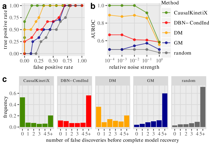
Figure 3: a, Median receiver operator curves (ROCs) for recovering the correct causal parents based on $500$ simulations. CausalKinetiX has the fastest recovery rate. b, Median area under the receiver operator curve (AUROC) for different relative noise levels, CausalKinetiX outperforms all other methods. c, Number of recoveries before all correct variables enter the model. In the majority of cases, CausalKinetiX has no false discovery.

Numerical stability, scalability, and misspecified models.

The method CausalKinetiX builds on standard statistical procedures, such as smoothing, quadratic programming, and regression. As opposed to standard nonlinear least squares, it does not make use of any numerical integration techniques. This avoids computational issues that arise when the dynamics result in stiff systems Shampine (2018). For each model, the runtime is less than cubic in the sample size, which means that the key computational cost is the exhaustive model search. We propose to use a screening step to reduce the number of possible models (SI 3 C), which allows applying the method to systems with hundreds of variables (e.g., metabolic network below). Moreover, it does not require any assumptions on the dynamics of the covariates. In this sense, the method is robust with respect to model misspecifications on the covariates that can originate from hidden variables or misspecified functional relationships. Consistency of the proposed variable ranking (SI 3), for example, only requires the model for the target variable to be correctly specified. Simulation experiments show that this robustness can be observed empirically (SI 4). Finally, there is empirical evidence that incorporating invariance can be interpreted as regularization preventing overfitting, and that the method is robust against correlated measurement error (SI 4).

Generalization in metabolic networks.

We apply the proposed method to a real biological data set of a metabolic network (Methods). Ion counts of one target variable and cell concentrations of 411 metabolites are measured at 11 time points across five different experimental conditions, each of which contains three biological replicates. The experiments include both up- and downshifts of the target variable, i.e., some of the conditions induce an increase of the target trajectory, compared to its starting value, other conditions induce a decrease.

We compare CausalKinetiX with the performance of nonlinear least squares (NONLSQ). To make the methods feasible to such a large dataset, we combine them with a screening based on DM. We thus call the method based on nonlinear least squares DM-NONLSQ; its parameters are estimated using the software Data2Dynamics (d2d) Raue et al. (2015), which uses CVODES of the SUNDIALS suite Hindmarsh et al. (2005) for numerical integration.

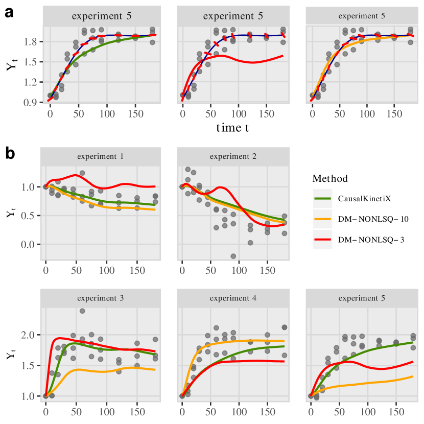
Figure 4: Metabolic network analysis. a, In-sample fit. All five experiments are used for model selection and parameter estimation. The plot shows model-based trajectories (numerically integrated) for experiment 5. DM with 10 terms (right) fits the data better than CausalKinetiX (left) or DM with 3 terms (middle). b, Out-of-sample fit. The plot shows the models’ ability to generalize to new experiments. Each plot shows model-based trajectories that are obtained when that experiment is not used for parameter estimation. CausalKinetiX shows the best generalization performance. The large DM model does not generalize well to unseen data due to overfitting.

Figure 4 (a) shows the models’ ability to describe the dynamics in the observed experiments (in-sample performance). DM-NONLSQ directly optimizes the residual sum of squares (RSS) and therefore fits the data better than CausalKinetiX, which takes into account stability, as well. The RSS for DM-NONLSQ-10 (based on 10 terms) is lower ($0.83$) compared to CausalKinetiX ($0.96$) averaged over all in-sample experiments. The plot contains diagnostics for analyzing kinetic models. The integrated dynamics are shown jointly with a smoother (blue) through the observations (grey). At the observed time points, the predicted derivatives (red lines) are also shown using smoothed $X$ and $Y$ values. Model fits that explain the data reasonably well in the sense that the integrated trajectory is not far from the observations, may predict derivatives (small red lines) on the smoother that do not agree well with the data: they fail to explain the underlying dynamics. For an example, see the in-sample-fit of DM-NONLSQ-10 in Figure 4 (a). We regard plotting a smoothing spline and the predicted derivatives for the fitted values as a highly informative tool when analyzing models for kinetic systems.

Pooling data across heterogeneous experiments, as, for example, done by DM-NONLSQ, is already a natural regularization technique; if there is sufficient heterogeneity in the data, the causal model is the only invariant model. Finitely many experiments, however, only exhibit limited heterogeneity and one can benefit from focusing specifically on invariant models. To compare the out-of-sample performance of the methods, we consider the best ranked model from Figure 4 a, hold out one experiment, fit the parameters on the remaining four experiments and predict the dynamics on the held out experiment. While DM-NONLSQ-10 explains the observations well in-sample, it does not generalize to the held out experiments. Neither does DM-NONLSQ-3 (based only $3$ terms) which avoids overfitting. The average RSS of the held-out experiments are $1.41$, $2.95$, and $3.45$ for CausalKinetiX, DM-NONLSQ-10, and DM-NONLSQ-3, respectively; see Figure 4 b. Another comparison, when the methods are fully agnostic about one of the experimental conditions is provided in SI 4. By trading off invariance and predictability, CausalKinetiX yields models that perform well on unseen experiments that have not been used for parameter estimation.

Discussion

In the natural sciences, differential equation modeling is a widely-used tool for describing kinetic systems. The discovery and verification of such models from data has become a fundamental challenge of science today. Existing methods are often based on standard model selection techniques or various types of sparsity enforcing regularization; they usually focus on predictive performance, and sometimes consider stability with respect to resampling (Meinshausen and Bühlmann, 2010; Basu et al., 2018). In this work, we develop novel methodology for structure search in ordinary differential equation models. Exploiting ideas from causal inference, we propose to rank models not only by their predictive performance, but also by taking into account invariance, i.e., their ability to predict well in different experimental settings. Based on this model ranking, we construct a ranking of individual variables reflecting causal importance. It provides researchers with a list of promising candidate variables that may be investigated further by performing interventional experiments, for example. Our ranking methodology (both for models and variables) comes with theoretical asymptotic guarantees and with a clear statement of the required assumptions. Extensive experimental evaluation on simulated data shows that our method is able to outperform current state-of-the art methods. Practical applicability of the procedure is further illustrated on a not yet published biological data set. Our implementation is readily available as an open-source R-package.

The principle of searching for invariant models opens up a promising direction for learning causal structure from realistic, heterogeneous datasets. The proposed CausalKinetiX framework is flexible in that it can be combined with a wide range of dynamical models and any parameter inference method. This is particularly relevant when the differential equations depend nonlinearly on the parameters. Future extensions may further include the extension to stochastic, partial and delay differential equations and the transfer to other areas of application like robotics, climate sciences, neuroscience and economics.

Methods

In this section, we provide additional details about data format, methodology and the experiments. We further prove that our method is statistically consistent, i.e., it infers correct models when the sample size grows towards infinity.

Data format

The data consist of $n$ repetitions of discrete time observations of the $d$ variables $\mathbf{X}$ (or their noisy version $\widetilde{\mathbf{X}}$) on the time grid $\mathbf{t}=(t_{1},\ldots,t_{L})$. Each of the repetitions is part of an experiment $\{e_{1},\ldots,e_{m}\}$. The experiments should be thought of as different states of the system and may stem from different interventions. One of the variables, $X^{1}$, say, is considered as the target, we write $Y_{t}^{1,(i)}=X_{t}^{1,i}$. We further assume an underlying dynamical model (which then results in various statistical dependencies between the variables and different time points).

Mass-action kinetic models

Many ODE based systems in biology are described by the law of mass-action kinetics. The resulting ODE models are linear combinations of various orders of interactions between the predictor variables $\mathbf{X}$. Assuming that the underlying ODE model of our target $Y=X^{1}$ is described by a version of the mass-action kinetic law, the derivative $\dot{Y}_{t}:=\frac{d}{dt}Y_{t}$ equals

$$\dot{Y}_{t}=g_{\theta}(\mathbf{X}_{t})=\sum_{k=1}^{d}\theta_{0,k}X^{k}_{t}+\sum_{j=1}^{d}\sum_{k=j}^{d}\theta_{j,k}X^{j}_{t}X^{k}_{t},$$ (2)

where $\theta=(\theta_{0,1},\dots,\theta_{0,d},\theta_{1,1},\theta_{1,2},\dots,\theta_{d,d})\in{\mathbb{R}}^{{d(d+1)}/{2}+d}$ is a parameter vector. We denote the subclass of all such linear models of degree $1$ consisting of at most $p$ terms (i.e., $p$ non-zero terms in the parameter vector $\theta$) by $\mathcal{M}^{\operatorname{Exhaustive}}_{p}$ and call these models exhaustive linear models of degree $1$. A more detailed overview of different collections of models is given in SI 2.

Model scoring

For each model $M$ the score $T=T(M)$ is computed using the following steps. They include fitting two models to the data: one in (M3) and the other one in (M4) and (M5).

1. Input: Data as described above and a collection $\mathcal{M}=\{M^{1},M^{2},\ldots,M^{m}\}$ of models over $d$ variables that is assumed to be rich enough to describe the desired kinetics. In the case of mass-action kinetics, e.g., $\mathcal{M}=\mathcal{M}^{\operatorname{Exhaustive}}_{p}$.

2. Screening of predictor terms (optional): For large systems, reduce the search space to less predictor terms. Essentially, any variable reduction technique based on the regression in step (M4) can be used. We propose using $\ell_{1}$-penalized regression (SI 2).

3. Smooth target trajectories: For each repetition $i\in\{1,\ldots,n\}$, smooth the (noisy) data $\widetilde{Y}^{(i)}_{t_{1}},\dots,\widetilde{Y}^{(i)}_{t_{L}}$ using a smoothing spline

   $$\hat{y}^{(i)}_{a}:=\operatorname*{argmin}_{y\in\mathcal{H}_{C}}\,\sum_{\ell=1}^{L}\big{(}\widetilde{Y}^{(i)}_{t_{\ell}}-y(t_{\ell})\big{)}^{2}+\lambda\int\ddot{y}(s)^{2}\,ds,$$ (3)

   where $\lambda$ is a regularization parameter, which in practice is chosen using cross-validation; $\mathcal{H}_{C}$ contains all smooth functions $[0,T]\rightarrow\mathbb{R}$, for which values and first two derivatives are bounded in absolute value by $C$. We denote the resulting functions by $\hat{y}^{(i)}_{a}:[0,T]\rightarrow{\mathbb{R}}$, $i\in\{1,\ldots,n\}$. For each of the $m$ candidate target models $M\in\mathcal{M}$ perform steps (M4)–(M6).

4. Fit candidate target model: For every $i\in\{1,\dots,n\}$, find the function $g^{i}\in\mathcal{G}$ s.t.

   $$\dot{Y}^{(k)}_{t}=g^{i}\big{(}\mathbf{X}^{(k)}_{t}\big{)}$$ (4)

   is satisfied as well as possible for all $t\in\mathbf{t}$ and for all repetitions $k$ belonging to a different experiment than repetition $i$. Below, we describe two procedures for this estimation step resulting in estimates $\hat{g}^{i}$. For each repetition $i\in\{1,\ldots,n\}$, this yields $L$ fitted values $\hat{g}^{i}(\widetilde{\mathbf{X}}^{(i)}_{t_{1}}),\dots,\hat{g}^{i}(\widetilde{\mathbf{X}}^{(i)}_{t_{L}})$. Leaving out the experiment of repetition $i$ ensures that only an invariant model leads to a good fit, as these predicted derivatives are only reasonable if the dynamics generalize across experiments.

5. Smooth target trajectories with derivative constraint: Refit the target trajectories for each repetition $i\in\{1,\ldots,n\}$ by constraining the smoother to these derivatives, i.e., find the functions $\hat{y}^{(i)}_{b}:[0,T]\rightarrow{\mathbb{R}}$ which minimize

   $$\begin{split}\hat{y}^{(i)}_{b}\coloneqq&\operatorname*{argmin}_{y\in\mathcal{H}_{C}}\sum_{\ell=1}^{L}\big{(}\widetilde{Y}^{(i)}_{t_{\ell}}-y(t_{\ell})\big{)}^{2}+\lambda\int\ddot{y}(s)^{2}\,ds,\\ &\text{such that}\quad\dot{y}(t_{\ell})=\hat{g}^{i}(\widetilde{\mathbf{X}}^{(i)}_{t_{\ell}})\text{ for all }{\ell}=1,\ldots,L.\end{split}$$ (5)

6. Compute score: If the candidate model $M$ allows for an invariant fit, the fitted values $\hat{g}^{i}(\widetilde{\mathbf{X}}^{(i)}_{1}),\dots,\hat{g}^{i}(\widetilde{\mathbf{X}}^{(i)}_{L})$ computed in (M4) will be reasonable estimates of the derivatives $\dot{Y}^{(i)}_{t_{1}},\dots,\dot{Y}^{(i)}_{t_{L}}$. This, in particular, means that the constrained fit in (M5) will be good, too. If, conversely, the candidate model $M$ does not allow for an invariant fit, the estimates produced in (M4) will be poor. We thus score the models by comparing the fitted trajectories $\hat{y}^{(i)}_{a}$ and $\hat{y}^{(i)}_{b}$ across repetitions as follows

   $$T(M)\coloneqq\frac{1}{n}\sum_{i=1}^{n}\left[\operatorname{RSS}_{b}^{(i)}-\operatorname{RSS}_{a}^{(i)}\right]/\left[\operatorname{RSS}_{a}^{(i)}\right],$$ (6)

   where $\operatorname{RSS}_{*}^{(i)}\coloneqq\frac{1}{L}\sum_{\ell=1}^{L}\big{(}\hat{y}^{(i)}_{*}(t_{\ell})-\widetilde{Y}^{(i)}_{t_{\ell}}\big{)}^{2}$. If there is a reason to believe that the observational noise has similar variances across experiments the division in the score can be removed to improve numerical stability.

The scores $T(M)$ induce a ranking on the models $M\in\mathcal{M}$, where models with a smaller score have more stable fits than models with larger scores. Below, we show consistency of the model ranking.

Variable ranking

The following method ranks individual variables according to their importance in obtaining invariant models. We score all models in the collection $\mathcal{M}$ based on their stability score $T(M)$ (see [13]) and then rank the variables according to how many of the top ranked models depend on them. This can be summarized in the following steps.

1. Input: same as in (M1).

2. Compute stabilities: For each model $M\in\mathcal{M}$ compute the non-invariance score $T(M)$ as described in [13]. Denote by $M_{(1)},\dots,M_{(K)}$ the $K$ top ranked models, where $K\in{\mathbb{N}}$ is chosen to be the number of expected invariant models in $\mathcal{M}$.

3. Score variables: For each variable $j\in\{1,\dots,d\}$, compute the following score

   $$s_{j}\coloneqq\frac{|\{k\in\{1,\dots,K\}\,|\,M_{(k)}\text{ depends on }j\}|}{K}.$$ (7)

   Here, “$M_{(k)}\text{ depends on }j$” means that the variable $j$ has an effect in the model $M_{(k)}$ (SI 2). If there are $K$ invariant models, the above score represents the fraction of invariant models that depend on variable $j$. It equals $1$ for variable $j$ if and only if every invariant model depends on that variable.

These scores $s^{j}$ are similar to what is referred to as inclusion probabilities in Bayesian model averaging Hoeting et al. (1999). Below, we construct hypothesis tests for the test whether a score is significantly higher than if the models are ranked randomly.

A natural choice for the parameter $K$ should equal the number of invariant models. This may be unknown in practice, but our empirical studies found that the method’s results are robust to the choice of $K$. In particular, we propose to choose a small $K$ to ensure that it is smaller than the number of invariant models (SI 2).

Fitting target models (M4)

In step (M4), for every $i\in\{1,\dots,n\}$, we perform a regression to find a function $g^{i}\in M$ such that [11] is optimized across all repetitions $k$ belonging to different experiments than $i$. This task is difficult for two reasons. First, the derivative values $\dot{Y}^{(k)}_{t}$ are not directly observed and, second, even if we had access to (noisy and unbiased versions of) $\dot{Y}^{(k)}_{t}$, we are dealing with an error-in-variables problem. Nevertheless, for certain model classes it is possible to perform this estimation consistently and since the predictions are only used as constraints, one expects estimates to work as long as they preserve the general dynamics. We propose two procedures: (i) a general method that can be adapted to many model classes and (ii) a method that performs better but assumes the target model to be linear in parameters.

The first procedure estimates the derivatives and then performs a regression based on the model class under consideration. That is, one fits the smoother $y_{a}^{(k)}$ from (M3) and then computes its derivatives. When using the first derivative of a smoothing spline it has been argued that the penalty term in [10] contains the third rather than the second derivative of $y$ Ramsay and Silverman (2005). We then regress the estimated derivatives on the data. As a regression procedure, one can use ordinary least squares if the models are linear or random forests, for example, if the functions are highly nonlinear.

The second method works for models that are linear in the parameters, i.e., for models that consist of functions of the form $g_{\theta}(\mathbf{x})=\sum_{j=1}^{p}\theta_{j}g_{j}(\mathbf{x})$, where the functions $g_{1},\dots,g_{p}$ are known transformations. This yields

$$Y_{t_{\ell}}^{(k)}-Y_{t_{\ell-1}}^{(k)}=\sum_{j=1}^{p}\theta_{j}\int_{t_{\ell-1}}^{t_{\ell}}g_{j}(\widetilde{\mathbf{X}}_{s}^{(k)})ds.$$

This approach does not require estimation of the derivatives of $Y$ but instead uses the integral of the predictors. It is well-known that integration is numerically more stable than differentiation Chen et al. (2017). Often, it suffices to approximate the integrals using the trapezoidal rule, i.e.,

$$\int_{t_{\ell-1}}^{t_{\ell}}g_{j}(\widetilde{\mathbf{X}}_{s}^{(k)})ds\approx\frac{g_{j}(\widetilde{\mathbf{X}}_{t_{\ell}}^{(k)})+g_{j}(\widetilde{\mathbf{X}}_{t_{\ell-1}}^{(k)})}{2}(t_{\ell}-t_{\ell-1}),$$

since the noise in the predictors is often stronger than the error in this approximation. The resulting bias is then negligible.

As mentioned above, most regression procedures have difficulties with errors-in-variables and therefore return biased results. Sometimes it can therefore be helpful to use smoothing or averaging of the predictors to reduce the impact of this problem. Our procedure is flexible in the sense that other fitting procedures, e.g., inspired by Ramsay et al. (2007); Oates et al. (2014); Calderhead et al. (2009), could be applied, too.

Experiment on metabolic network

Defining the auxiliary variable $Z_{t}:=2-Y_{t}$, we expect that the target species $Y_{t}$ and $Z_{t}$ are tightly related: $Y_{t}\rightleftharpoons Z_{t}$, i.e., $Y_{t}$ is formed into $Z_{t}$ and vice versa. We therefore expect models of the form

$$\dot{Y}_{t} =\theta_{1}Z_{t}X_{t}^{j}X_{t}^{k}+\theta_{2}Z_{t}X_{t}^{p}X_{t}^{q}-\theta_{3}Y_{t}X_{t}^{r}X_{t}^{s}$$

$$\dot{Z}_{t} =-\theta_{1}Z_{t}X_{t}^{j}X_{t}^{k}-\theta_{2}Z_{t}X_{t}^{p}X_{t}^{q}+\theta_{3}Y_{t}X_{t}^{r}X_{t}^{s},$$

where $j,k,p,q,r,s\in\{1,\ldots,411\}$ and $\theta_{1},\theta_{2},\theta_{3}\geq 0$. By the conservation of mass both target equations mirror themselves, which makes it sufficient to only learn the model for $Y_{t}$. More precisely, we use the model class consisting of three term models of the form $Z_{t}X_{t}^{j}X_{t}^{k}$, $Y_{t}X_{t}^{j}X_{t}^{k}$, $Z_{t}X_{t}^{j}$, $Y_{t}X_{t}^{j}$, $Z_{t}$, or $Y_{t}$, where the sign of the parameter is constrained to being positive or negative depending on whether the term contains $Z_{t}$ or $Y_{t}$, respectively. We constrain ourselves to three terms, as we found this to be the smallest number of terms that results in sufficiently good in-sample fits. Given sufficient computational resources, one may include more terms, too, of course. The sign constraint can be incorporated into our method by performing a constrained least squares fit instead of OLS in step (M4). This constrained regression can then be solved efficiently by a quadratic program with linear constraints.

As the biological data is high-dimensional, our method first screens down to $100$ terms and then searches over all models consisting of $3$ terms. To get more accurate fits of the dynamics, we pool and smooth over the three biological replicates and only work with the smoothed data.

Significance of variable ranking

We can test whether a given score $s_{j}$, defined in [14], is significant in the sense that the number of top ranked models depending on variable $j$ is higher than one would expect if the ranking of all models in $\mathcal{M}$ was random. More precisely, consider the null hypothesis

$$H_{0}:\quad\begin{array}[]{l}\text{the top ranked models }M_{(1)},\dots,M_{(K)}\\ \text{are drawn uniformly from all models in }\mathcal{M}.\end{array}$$

It is straightforward to show that under $H_{0}$ it holds that $K\cdot s_{j}$ follows a hypergeometric distribution with parameters $\lvert\mathcal{M}\rvert$ (population size), $\lvert\{M\in\mathcal{M}\,|\,M\text{ depends on }j\}\rvert$ (number success in population) and $K$ (number of draws). For each variable we can hence compute a $p$-value to assess whether it is significantly important for stability.

Theoretical consistency guarantees

We prove that both the model ranking and the proposed variable ranking satisfy theoretical consistency guarantees. More precisely, under suitable conditions and in the asymptotic setting where both the number of realizations $n$ and the number of time points $L$ converge to infinity, every invariant model will be ranked higher than all non-invariant models. Given sufficient heterogeneity of the experiments it additionally holds that the variable score $s_{j}$ defined in [14] tends to one if and only if $j\in S^{*}$, see [1]. Details and proofs are provided in SI 3.

Relation to causality

Causal models enable us to model a system’s behavior not only in an observational state, but also under interventions. There are various ways to define causal models (Pearl, 2009; Imbens and Rubin, 2015). The concept of structural causal models is well-suited for the setting of this paper and its formalism can be adapted to the case of dynamical models (SI 1). If the experimental settings correspond to different interventions on variables other than $Y$, choosing $S^{*}$ as the set of causal parents of $Y$ satisfies [1]. If the settings are sufficiently informative, no other set satisfies [1].

Code and data availability

Well-documented code is available as an open source R package on CRAN (https://cran.r-project.org/web/packages/CausalKinetiX). It includes the ODE models used in the simulations, e.g., the Maillard reaction. More details, e.g., about reproducing all figures and a ported python version of the package are available at http://www.causalkinetix.org.

Supplementary Information

The supporting material is divided into the following 4 parts:

• Supplementary information A: Causality

• Supplementary information B: CausalKinetiX for parametric dynamical models

• Supplementary information C: Consistency result and proof

• Supplementary information D: Extended empirical results

Appendix A Causality

This supplementary note contains details on causal models and the relationship between CausalKinetiX and causality. It accompanies the article Learning stable and predictive structures in kinetic systems.

A.1 Structural causal models

We first revise the widely used concept of structural causal models [Pearl, 2009] for i.i.d. data without any time structure. A structural causal model (SCM) over $d$ random variables $X^{1},\ldots,X^{d}$ consists of $d$ assignments

$$X^{j}:=f^{i}(X^{{\mathbf{PA}}_{j}},\varepsilon^{j}),\quad j=1,\ldots,d$$

together with a noise distribution over the random vector $(\varepsilon^{1},\ldots,\varepsilon^{d})$, which we may assume to factorize, implying that the noise variables are independent. Here, ${\mathbf{PA}}_{j}\subseteq\{1,\ldots,d\}$ are called the (causal) parents of $j$. For each SCM we obtain a corresponding graph over the vertices $(1,\ldots,d)$ by drawing edges from ${\mathbf{PA}}_{j}$ to $j$, $j\in\{1,\ldots,d\}$. The corresponding directed graph is assumed to be acyclic. Under these conditions, the SCM can be shown to entail an observational distribution over $X^{1},\ldots,X^{d}$.

An intervention now corresponds to replacing one of these assignments, such that the resulting graph is again acyclic. This ensures that the new SCM again entails a joint distribution over $X^{1},\ldots,X^{d}$, the intervention distribution. If $X^{k}:=f^{k}(X^{{\mathbf{PA}}_{k}},\varepsilon^{k})$ is replaced by $X^{k}:=4$, for example, that distribution is sometimes denoted by $do(X^{k}:=4)$, the $do$-notation indicating that a variable has been intervened on (rather than conditioned on).

The above concept of SCMs can be straightforwardly adapted to dynamical systems. A causal kinetic model over a process $\mathbf{X}:=(\mathbf{X}_{t})_{t}:=(X^{1}_{t},\ldots,X^{d}_{t})_{t}$ is a collection of $d$ assignments

$$\dot{X}_{t}^{1} :=f^{1}(X_{t}^{{\mathbf{PA}}_{1}}),\qquad X^{1}_{0}:=x^{1}_{0}$$

$$\dot{X}_{t}^{2} :=f^{2}(X_{t}^{{\mathbf{PA}}_{2}}),\qquad X^{2}_{0}:=x^{2}_{0}$$

$$\;\;\;\vdots$$

$$\dot{X}_{t}^{d} :=f^{d}(X_{t}^{{\mathbf{PA}}_{d}}),\qquad X^{d}_{0}:=x^{d}_{0},$$

where $\dot{X}_{t}^{j}$ is short-hand notation for $\frac{d}{dt}{X}_{t}^{j}$. As above, ${\mathbf{PA}}_{j}\subseteq\{1,\ldots,d\}$ are called the direct (or causal) parents of $X^{j}$. We explicitly allow for cycles in the corresponding graph (in particular, a node might be its own parent), but require the above system of differential equations to be solvable. Furthermore, we may assume observations from the above system are corrupted by observational noise, e.g., $\widetilde{\mathbf{X}}_{t}=\mathbf{X}_{t}+\boldsymbol{\varepsilon}_{t}$.

As in the i.i.d. case, an intervention replaces one (or more) of the above assignments. The change may include the initial values, the differential equation or both at the same time. Formally, an intervention replaces the $k$th assignment with

$$X^{k}_{0}:=\xi\quad\text{or}\quad\dot{X}^{k}_{t}:=g(X_{t}^{{\mathbf{PA}}},X^{k}_{t}),$$

with ${\mathbf{PA}}$ being the new set of parents of $j$. In either case, the system of differential equations is still required to be solvable. In the presence of observational noise, the noise is assumed to enter after the intervention. Similar frameworks have been suggested [Mooij et al., 2013, Blom and Mooij, 2018, Rubenstein et al., 2018], which usually focus more on the equilibrium state of the system. The above framework allows for a variety of interventions, such as setting a variable $X^{k}$ to a constant $c$, for example, or “pulling” a variable $X^{k}$ to a certain value $c$. One can change the dependence of a variable on its parents or change the parent set of $X^{k}$ completely. In the case of mass-action kinetics, a change in reaction rates can be modeled as an intervention, for example.

A.2 Stability of causal models

In this work, we assume that we are given a target variable $Y_{t}$ and a set $\mathbf{X}_{t}$ of $d$ predictors. Suppose that there is an underlying causal kinetic model (see Section A.1) over the process $(\mathbf{X}_{t},Y_{t})$. If we consider experimental conditions that correspond to different interventions on variables other than $Y$, it follows that $S^{*}:={\mathbf{PA}}_{Y}$ yields a stable model, i.e.,

$$\dot{Y}^{(i)}_{t}=f\big{(}{X}^{S^{*},(i)}_{t}\big{)},\,\text{ for all }i=1,\ldots,n,$$

see [1] in the main article and B below. This principle is known as autonomy or modularity, see Aldrich [1989], Haavelmo [1944], Pearl [2009], Schölkopf et al. [2012], for example.

A.3 Causality through stability

The above mentioned stability property of the parents of $Y$ can be exploited for causal discovery. Suppose that there is an underlying causal kinetic model, whose structure is unknown. Suppose further, that we are given data from different experimental settings and that the parents of $Y$ satisfy the above stability. We can then search for all sets $S\subseteq\{1,\ldots,d\}$, such that $\dot{Y}^{(i)}_{t}=f({X}^{S,(i)}_{t})$, for all $i=1,\ldots,n$. There can be more than one invariant (or stable) set, but by assumption the set of parents is one of these sets. It has been proposed to output the intersection of all invariant sets, which is guaranteed to be a subset of the causal parents [Meinshausen et al., 2016, Peters et al., 2016]. The intersection itself, however, does not necessarily lead to a model with good predictive performance. In CausalKinetiX, we propose to use a trade-off between stability and predictability. This yields models that generalize well to unseen experimental conditions. If there are sufficiently many and informative experimental conditions, the causal parents of $Y$ are the unique set satisfying the invariance condition. (This is, trivially, the case if all variables other than $Y$ are intervened on, for example.) Under such conditions, the consistency results we develop in C then state that CausalKinetiX in the limit of infinite sample size indeed recovers the set of causal parents of $Y$, see Theorem 1 below.

Appendix B CausalKinetiX for parametric dynamical models

This supplementary note contains details on the different types of model classes that can be used in the CausalKinetiX framework. Additionally, we give details on how to choose the tuning parameter $K$ in the variable ranking and propose to explicit screening procedures. It accompanies the article Learning stable and predictive structures in kinetic systems.

B.1 Connection between models and variables

Given a differential equation $\dot{Y}_{t}=g(\mathbf{X}_{t})$ it will be convenient to speak about the arguments $\mathbf{X}_{t}$ of the function $g$ that have an influence on the outcome $\dot{Y}_{t}$. For any set $S\subseteq\{1,\dots,d\}$, we therefore define

$$\mathcal{F}(S)\coloneqq\left\{g:{\mathbb{R}}^{d}\rightarrow{\mathbb{R}}\,\big{|}\,\exists f:{\mathbb{R}}^{\lvert S\rvert}\rightarrow{\mathbb{R}}:\forall\mathbf{x}\in{\mathbb{R}}^{d}\;g(\mathbf{x})=f(\mathbf{x}^{S})\right\}.$$

A set of functions $M\subseteq\mathcal{F}(S)$ (also referred to as model), then contains only functions that do not depend on variables outside $S$. In the class of mass-action kinetics, for example, we could have

$$M_{1} =\{g\,|\,g(x)=\theta_{1}x_{1}+\theta_{7}x_{7},\text{ where }\theta_{1},\theta_{7}\in\mathbb{R}\},$$

$$M_{2} =\{g\,|\,g(x)=\theta_{2}x_{2}+\theta_{3}x_{3},\text{ where }\theta_{2},\theta_{3}\in\mathbb{R}\},$$

which implies $M_{1}\subseteq\mathcal{F}(\{1,7\})$ and $M_{2}\subseteq\mathcal{F}(\{2,3\})$, see Section B.2 for more details. In practice, the underlying structure is unknown and many methods therefore include a model selection step. Here, we assume that we are given a family of target models $\mathcal{M}=\{M^{1},\dots,M^{m}\}$, where individual models can depend on various different subsets of variables $S\subseteq\{1,\dots,d\}$. We say a model $M\text{ depends on }j$ if there is no $S\subseteq\{1,\ldots,d\}$ with $j\notin S$ and $M\subseteq\mathcal{F}(S)$. Furthermore, we refer to $M$ as a target model and to $\mathcal{M}$ as a collection of target models. Based on these definitions, we can make precise what it means for the target trajectories $Y$ to be described by invariant dynamics.

Assumption 1 (invariance).

There exists a set $S^{*}$ and a function $f^{*}:\mathbb{R}^{|S^{*}|}\rightarrow\mathbb{R}$ satisfying for all $i\in\{1,\ldots,n\}$ and all $t\in\mathbf{t}$ that

$$\dot{Y}^{(i)}_{t}=f^{*}\big{(}\mathbf{X}^{S^{*},(i)}_{t}\big{)}.$$ (8)

Further, $S^{*}$ is minimal for $f^{*}$ in the following sense: there is no $S\subsetneq S^{*}$ such that $f^{*}\in\mathcal{F}(S)$.

For causal kinetic models, the pair $(f^{Y},{\mathbf{PA}}_{Y})$ satisfies Assumption 1 whenever the environments consist of interventional data, which do not contain interventions on the target $Y$ itself. Even if Assumption 1 is satisfied the pair $(f^{*},S^{*})$ is not necessarily unique, i.e., there may be one or several pairs satisfying [8]. In general, both the set $S^{*}$ as well as the invariant function $f^{*}$ are of interest in practice as both are strongly related to the causal mechanisms of the underlying system.

B.2 Parametric models for mass-action kinetics

Many ODE based systems in biology are described by the law of mass-action kinetics. The resulting ODE models are linear combinations of various orders of interactions between the predictor variables $\mathbf{X}$. Assuming that the underlying ODE model of our target $Y$ is described by a version of the mass-action kinetic law, the derivative $\dot{Y}_{t}$ equals

$$\dot{Y}_{t}=g_{\theta}(\mathbf{X}_{t})=\sum_{k=1}^{d}\theta_{0,k}X^{k}_{t}+\sum_{j=1}^{d}\sum_{k=j}^{d}\theta_{j,k}X^{j}_{t}X^{k}_{t},$$ (9)

where $\theta=(\theta_{0,1},\dots,\theta_{0,d},\theta_{1,1},\theta_{1,2},\dots,\theta_{d,d})\in{\mathbb{R}}^{{d(d+1)}/{2}+d}$ is a parameter vector. Correspondingly, the function on the right-hand side of [8] in Assumption 1 has such a parametric form, too. The assumption that the model only depends on the variables in $S^{*}$ can be expressed by a sparsity on the parameter $\theta$, i.e., $\theta_{j,k}=0$ for all $j,k$ with $j\notin S^{*}$ or $k\notin S^{*}$. A target model $M$ can be constructed by a sparsity pattern. Formally, such a sparsity pattern is described by a vector $v\in\{0,1\}^{{d(d+1)}/{2}+d}$ which specifies the zero entries in $\theta$. For every such $v$, we define

$$M^{v}\coloneqq\Big{\{}g_{\theta}:{\mathbb{R}}^{d}\rightarrow{\mathbb{R}}\,\Big{|}\,\forall\mathbf{x}\in{\mathbb{R}}^{d}:g_{\theta}(\mathbf{x})=\sum_{k,j}\theta_{k,j}x^{k}x^{j}\text{ and }v*\theta=\theta\Big{\}},$$

where $*$ denotes the element-wise product. In principle, one could now search over all sparsity patterns of $\theta$, i.e., define $\mathcal{M}=\{M^{v},v\in\{0,1\}^{{d(d+1)}/{2}+d}\}$, but this becomes computationally infeasible already for small values of $d$. In this work, we suggest two different collections of target models. Other choices, in particular those motivated by prior knowledge, are possible, too, and can easily be included in our framework.

Exhaustive models.

Using only the constraint on the number of terms $p$ leads to the following collection of models

$$\mathcal{M}^{\operatorname{Exhaustive}}_{p}=\left\{M^{v}\,\big{|}\,v\text{ has at most }p\text{ non-zeros}\right\}.$$

Every model in $\mathcal{M}^{\operatorname{Exhaustive}}_{p}$ consists of a linear combination of a fixed number of at most $p$ terms of the form $X^{1},\dots,X^{d},X^{1}X^{1},X^{1}X^{2},\ldots,X^{d-1}X^{d}$ or $X^{d}X^{d}$.

Main effect models.

Alternatively, one can also add the restriction that the models including interaction terms for variables, include the corresponding main effects, too.

$$\mathcal{M}^{\operatorname{MainEffect}}_{p}=\big{\{}M^{v}\,\big{|}\, v\text{ has at most }p\text{ non-zeros and }$$

$$v_{0,j}\neq 0\text{ implies }v_{k,j}\neq 0\,\forall k<j\text{ and }v_{j,k}\neq 0\,\forall k\geq j\big{\}}.$$

While the number of main effect models is much smaller it generally requires to fit larger models, which can lead to overfitting. For example, if the true invariant model only depends on the two terms $X^{1}$ and $X^{4}X^{5}$ there exists a exhaustive model with two parameters that is invariant, while the smallest main effect model has nine parameters.

B.3 Screening procedures and choosing parameter $K$ in variable selection

Screening of terms (M2)

For large scale applications, e.g., when $d$ is larger than $30$, the computational complexity of the method can be significantly reduced by including a prior screening step. The collections of models from mass-action kinetics scale as

$$\lvert\mathcal{M}^{\operatorname{Exhaustive}}_{p}\rvert=\sum_{k=1}^{p}\binom{\tbinom{d}{2}}{k}=\mathcal{O}(d^{2p}).$$

Even though computation of the stability score for a single model is fast, this shows that an exhaustive search is infeasible for settings with large $d$. We propose to reduce the model size by a screening step that screens terms that are useful for prediction in the model estimation in (M4) then continue our procedure with the reduced model class. This procedure allows the method to be applied in high-dimensional settings.

Usually, the screening step will focus on predictability, and any screening or variable selection method based on the model fit (see [11]) can be used. We provide two explicit options based on $\ell^{1}$-penalized least squares, also known as Lasso Tibshirani [1994]. The first method performs the regularization on the level of the derivatives (gradient matching GM) and the second on the integrated problem (difference matching DM), see SI 4, Section D.1. These two options can be used as screening steps, even in combination with other methods, such as nonlinear least squares (NONLSQ), or as parameter estimation methods in themselves. Even though we are not aware of any work that proposes this precise implementation, the idea of using $\ell^{1}$-penalized procedures for model inference has been used extensively Boninsegna et al. [2018], Brunton et al. [2016], Mikkelsen and Hansen [2017], Rudy et al. [2017], Schaeffer [2017], Szederkényi et al. [2011], Tran and Ward [2017], Wu et al. [2014].

Choosing parameter $K$ in variable ranking (V2)

Ideally, as mentioned in (V2), $K$ should equal the number of invariant models, see also the consistency results in SI 3. In our empirical studies, we found that the method’s results are robust to the choice of $K$. In general, we propose to choose a small $K$ to ensure that it is smaller than the number of invariant models. Depending on the collection $\mathcal{M}$ of target models it is sometimes possible to give a heuristic number of invariant models. For example in the case of mass-action kinetics, we have the following reasoning for the exhaustive models $\mathcal{M}^{\operatorname{Exhaustive}}_{p+1}$. If the smallest invariant model only has $p$ terms (i.e., it corresponds to a $v^{*}\in V_{p+1}$ with $\sum_{j}v^{*}_{j}=p$), it follows that any super-model (i.e., any $v\in V_{p+1}$ with $\sum_{j}\lvert v_{j}-v^{*}_{j}\rvert=1$) is also an invariant model. The number of super-models, however, is given by $2d+\binom{d}{2}-p$. Hence, if we use the model collection $\mathcal{M}^{\operatorname{Exhaustive}}_{p+1}$, where $p$ is assumed to be the expected number of terms contained in the smallest invariant model, a reasonable choice is to set $K=2d+\binom{d}{2}-p$.

Appendix C Consistency result and proof

This supplementary note contains the precise formulation of the consistency result mentioned in the article Learning stable and predictive structures in kinetic systems as well as a detailed proof. For completeness and to ensure better understanding, we first recall all details required for a precise formulation of the result (Section C.1 and Section C.2) and then present the detailed proof (Section C.3).

C.1 Detailed procedure

In this section, we recall the step-wise procedures for model scoring and variable ranking. Note, that the version of the model ranking presented in Section C.1.1 is slightly different from the one in the main article. More specifically, step (M4) does not leave out experiments but rather pools across all experiments. This allows for a simpler theoretical analysis but neglects the additional stability. However, we believe that the theory also holds for the more complicated leave-one-out procedure and actually expect it to have better finite sample properties.

C.1.1 Model scoring

For each model $M$ the score $T=T(M)$ is computed as follows.

1. Input: Data as described above and a collection $\mathcal{M}=\{M^{1},M^{2},\ldots,M^{m}\}$ of models over $d$ variables that is assumed to be rich enough to describe the desired kinetics. In the case of mass-action kinetics, examples include $\mathcal{M}=\mathcal{M}^{\operatorname{MainEffect}}_{p}$ or $\mathcal{M}=\mathcal{M}^{\operatorname{Exhaustive}}_{p}$.

2. Screening of predictor terms (optional): For large systems, reduce the search space to less predictor terms. This replaces the collection of models by a smaller collection, which we again denote by $\mathcal{M}$.

3. Smooth target trajectories: For each repetition $i\in\{1,\ldots,n\}$, smooth the (noisy) data $\widetilde{Y}^{(i)}_{t_{1}},\dots,\widetilde{Y}^{(i)}_{t_{L}}$ using a smoothing spline

   $$\hat{y}^{(i)}_{a}:=\operatorname*{argmin}_{y\in\mathcal{H}_{C}}\,\sum_{\ell=1}^{L}\big{(}\widetilde{Y}^{(i)}_{t_{\ell}}-y(t_{\ell})\big{)}^{2}+\lambda\int\ddot{y}(s)^{2}\,ds,$$ (10)

   where $\lambda$ is a regularization parameter, which in practice is chosen using cross-validation; $\mathcal{H}_{C}$ contains all smooth functions $[0,T]\rightarrow\mathbb{R}$, for which values and first two derivatives are bounded in absolute value by $C$. We denote the resulting functions by $\hat{y}^{(i)}_{a}:[0,T]\rightarrow{\mathbb{R}}$, $i\in\{1,\ldots,n\}$. For each of the $m$ candidate target models $M\in\mathcal{M}$ perform the steps (M4)–(M6).

4. Fit candidate target model: Fit the target model $M$, i.e., find the best fitting function $g\in M$ such that

   $$\dot{Y}^{(i)}_{t}=g\big{(}\mathbf{X}^{(i)}_{t}\big{)},$$ (11)

   holds for all $i\in\{1,\dots,n\}$ and $t\in\mathbf{t}$. Below, we describe two procedures for this estimation step resulting in an estimate $\hat{g}$. For each repetition $i\in\{1,\ldots,n\}$, this yields $L$ fitted values $\hat{g}(\widetilde{\mathbf{X}}^{(i)}_{t_{1}}),\dots,\hat{g}(\widetilde{\mathbf{X}}^{(i)}_{t_{L}})$.

5. Smooth target trajectories with derivative constraint: Refit the target trajectories for each repetition $i\in\{1,\ldots,n\}$ by constraining the smoother to these derivatives, i.e., find the functions $\hat{y}^{(i)}_{b}:[0,T]\rightarrow{\mathbb{R}}$ which minimize

   $$\begin{split}\hat{y}^{(i)}_{b}\coloneqq&\operatorname*{argmin}_{y\in\mathcal{H}_{C}}\sum_{\ell=1}^{L}\big{(}\widetilde{Y}^{(i)}_{t_{\ell}}-y(t_{\ell})\big{)}^{2}+\lambda\int\ddot{y}(s)^{2}\,ds,\\ &\text{such that}\quad\dot{y}(t_{\ell})=\hat{g}(\widetilde{\mathbf{X}}^{(i)}_{t_{\ell}})\text{ for all }{\ell}=1,\ldots,L.\end{split}$$ (12)

6. Compute score: If the candidate model $M$ allows for an invariant fit, the fitted values $\hat{g}(\widetilde{\mathbf{X}}^{(i)}_{1}),\dots,\hat{g}(\widetilde{\mathbf{X}}^{(i)}_{L})$ computed in (M4) will be reasonable estimates of the derivatives $\dot{Y}^{(i)}_{t_{1}},\dots,\dot{Y}^{(i)}_{t_{L}}$. This, in particular, means that the constrained fit in (M5) will be good, too. If, conversely, the candidate model $M$ does not allow for an invariant fit, the estimates produced in (M4) will be poor. We thus score the models by comparing the fitted trajectories $\hat{y}^{(i)}_{a}$ and $\hat{y}^{(i)}_{b}$ across repetitions as follows

   $$T(M)\coloneqq\frac{1}{n}\sum_{i=1}^{n}\left[\lvert\operatorname{RSS}_{b}^{(i)}-\operatorname{RSS}_{a}^{(i)}\rvert\right]/\left[\operatorname{RSS}_{a}^{(i)}\right],$$ (13)

   where $\operatorname{RSS}_{*}^{(i)}\coloneqq\frac{1}{L}\sum_{\ell=1}^{L}\big{(}\hat{y}^{(i)}_{*}(t_{\ell})-\widetilde{Y}^{(i)}_{t_{\ell}}\big{)}^{2}$.

The scores $T(M)$ induce a ranking on the models in $\mathcal{M}$, where models with a smaller score have more stable fits than models with larger scores. Below, we show consistency of the model ranking.

C.1.2 Variable ranking

The following idea ranks individual variables according to their importance in stabilizing models. We score all models in the collection $\mathcal{M}$ based on their stability as described above and then rank the variables according to how many of the top ranked models depend on them. This can be summarized in the following steps.

1. Input: same as in (M1).

2. Compute stabilities: For each model $M\in\mathcal{M}$ compute the stability score $T(M)$ as described in [13]. Denote by $M_{(1)},\dots,M_{(K)}$ the $K$ top ranked models, where $K\in{\mathbb{N}}$ is chosen to be the number of expected invariant models in $\mathcal{M}$. See below for how to choose $K$ in practice.

3. Score variables: For each variable $j\in\{1,\dots,d\}$ compute the following score

   $$s_{j}\coloneqq\frac{|\{k\in\{1,\dots,K\}\,|\,M_{(k)}\text{ depends on }j\}|}{K}.$$ (14)

   Here, “$M_{(k)}\text{ depends on }j$” means that there is no $S\subseteq\{1,\ldots,d\}$ with $j\notin S$ and $M_{(k)}\subseteq\mathcal{F}(S)$. If there are exactly $K$ invariant models, the above score then represents the fraction of invariant models that depend on variable $j$. In particular, it equals $1$ for a variable $j$ if and only if every invariant model depends on that variable.

C.2 Consistency of ranking procedure

First, we recall the key concept of invariance, which will be an important condition in order for our consistency result to hold.

Assumption 2 (invariance).

There exists a set $S^{*}$ and a function $f^{*}:\mathbb{R}^{|S^{*}|}\rightarrow\mathbb{R}$ satisfying for all $i\in\{1,\ldots,n\}$ and all $t\in\mathbf{t}$ that

$$\dot{Y}^{(i)}_{t}=f^{*}\big{(}\mathbf{X}^{S^{*},(i)}_{t}\big{)}.$$

Further, $S^{*}$ is minimal for $f^{*}$ in the following sense: there is no $S\subsetneq S^{*}$ such that $f^{*}\in\mathcal{F}(S)$.

Next, we provide conditions under which the proposed procedure is consistent. To this end, we fix the number of environments (or experiments) to $m$ and assume that there exist $R$ repetitions for each experiment observed on $L$ time points. In total this means we observe $n=m\cdot R$ trajectories, each on a grid of $L$ time points. As asymptotics, consider a growing number of repetitions $R_{n}$ and simultaneously a growing number of time points $L_{n}$. Here, increasing repetitions $R$ and time points $L$ corresponds to collecting more data and obtaining a finer time resolution, respectively. Both of these effects are achieved by novel data collection procedures. To make this more precise, assume that for each $n\in{\mathbb{N}}$, we are given a time grid

$$\mathbf{t}_{n}=(t_{n,1},\ldots,t_{n,L_{n}})$$

on which the data are observed and such that $L_{n}\rightarrow\infty$ for $n\rightarrow\infty$. For simplicity we will only analyze the case of a uniform grid, i.e., we assume that $\Delta t\coloneqq t_{n,k+1}-t_{n,k}=\frac{1}{L_{n}}$ for all $k\in\{1,\dots,L_{n}\}$. We denote the $m$ environments by $e_{1},\dots,e_{m}\subseteq\{1,\dots,n\}$ and assume for all $k\in\{1,\dots,m\}$ that $\lvert e_{k}\rvert=R_{n}$ which grows as $n$ increases.

To achieve consistency of our ranking procedures (both for models and variables) we require the following three conditions (C1)–(C3) below. These three conditions should be understood as high-level conditions or guidelines. There may be, of course, other sufficient assumptions that yield the desired result and that might cover other settings and models.

1. Consistency of target smoothing: The smoothing procedure in (M3), see Section C.1.1, satisfies the following consistency: For all $k\in\{1,\dots,m\}$ it holds that

   $$\lim_{n\rightarrow\infty}{\mathbb{E}}\left(\sup_{t\in[0,T]}\left(\hat{y}^{(e_{k})}_{a}(t)-Y^{(e_{k})}_{t}\right)^{2}\right)=0,$$

   where, by slight abuse of notation, the superscript $(e_{k})$ denotes a fixed repetition from the environment $e_{k}$.

2. Consistency of model estimation: For every invariant model $M\in\mathcal{M}$, let $\hat{g}_{n}$ be the estimate from (M4). Then, for all $k\in\{1,\dots,m\}$ it holds that

   $$L_{n}\max_{\ell\in\{1,\dots,L_{n}\}}\lvert\hat{g}_{n}(\widetilde{\mathbf{X}}^{(e_{k})}_{t_{n,\ell}})-\dot{Y}^{(e_{k})}_{t_{n,\ell}}\rvert\overset{{\mathbb{P}}}{\longrightarrow}0$$

   as $n\rightarrow\infty$, i.e., the estimation procedure $\hat{g}_{n}$ in (M4) is consistent. Furthermore, for all non-invariant models $M\in\mathcal{M}$ there exists a smooth function $g\in M$ such that $g$ and its first derivative are bounded and it holds for all $t\in[0,T]$ and for all $k\in\{1,\dots,m\}$ that

   $$L_{n}\max_{\ell\in\{1,\dots,L_{n}\}}\lvert\hat{g}_{n}(\widetilde{\mathbf{X}}^{(e_{k})}_{t_{\ell}})-g(\mathbf{X}^{(e_{k})}_{t_{\ell}})\rvert\overset{{\mathbb{P}}}{\longrightarrow}0$$

   as $n\rightarrow\infty$, i.e., the estimation convergences to a fixed function.

3. Uniqueness of invariant model: There exists a unique function $g^{*}\in\cup_{M\in\mathcal{M}}M$ and a unique set $S^{*}\subseteq\{1,\dots,d\}$ such that for all $n\in\{m,m+1,\dots\}$ the pair $f^{*}(\mathbf{x})\coloneqq g^{*}(\mathbf{x}^{S^{*}})$ and $S^{*}$ satisfy Assumption 2. This condition is fulfilled if the experiments are sufficiently heterogeneous, e.g., because there are sufficiently many and strong interventions.

Note that (C2) relates to the problem of error-in-variables. Relying on the conditions (C1)–(C3), we are now able to prove consistency results for both the model ranking from Section C.1.1 and the variable ranking from Section C.1.2. Recalling the definition of $T_{n}(M)$ given in [13] (small values of $T_{n}(M)$ indicate invariance), we define

$$\operatorname{RankAccuracy}_{n}\coloneqq 1-\frac{\big{|}\{M\in\mathcal{M}\,|\,T_{n}(M)<\max_{\{\tilde{M}\in\mathcal{M}\mid\tilde{M}\text{ invariant}\}}T_{n}(\tilde{M})\text{ and }M\text{ not invariant}\}\big{|}}{\big{|}\{M\in\mathcal{M}\,|\,M\text{ not invariant}\}\big{|}}$$ (15)

as performance measure of our model ranking. RankAccuracy is thus equal to $1$ minus “proportion of non-invariant models that are ranked better than the worst invariant model”. In particular, it equals $1$ if and only if all invariant models are ranked better than all other models. If the collection $\mathcal{M}$ contains no invariant models, we define the RankAccuracy to be $1$. Given the above conditions the following consistency holds.

Theorem 1 (rank consistency).

Let Assumption 2 and conditions (C1) and (C2) be satisfied. Additionally, assume that for all $k\in\{1,\dots,m\}$ it holds for all $i\in e_{k}$ and $\ell\in\{1,\dots,L_{n}\}$ that the noise variables $\varepsilon_{t_{\ell}}^{(i)}$ are i.i.d., symmetric, sub-Gaussian and satisfy ${\mathbb{E}}(\varepsilon_{t_{\ell}}^{(i)})=0$ and ${\mathbf{var}}(\varepsilon_{t_{\ell}}^{(i)})=\sigma^{2}_{k}$. Let $Y_{t}$ and its first and second derivative be bounded and assume that for all non-invariant sets $M\in\mathcal{M}$ the sets $\{t\mapsto g(X_{t})\,|\,g\in M\}$ are closed with respect to the supremum norm. Then, it holds that

$$\lim_{n\rightarrow\infty}{\mathbb{E}}\left(\operatorname{RankAccuracy}_{n}\right)=1.$$

If, in addition, condition (C3) holds, we have the following guarantee for the variable scores $s_{j}^{n}=s_{j}$, defined in [14]:

• for all $j\in S^{*}$ it holds that $\lim_{n\rightarrow\infty}{\mathbb{E}}(s^{n}_{j})=1$ and

• for all $j\not\in S^{*}$ it holds that $\lim_{n\rightarrow\infty}{\mathbb{E}}(s^{n}_{j})\leq\frac{K-1}{K}$,

where $K:=\lvert\{M\in\mathcal{M}\,|\,M\text{ is invariant}\}\rvert$.

The result is proved in the following section, which also contains the choice of $C$ for (M3). Note that if screening is used, condition (C3) can only be satisfied if the screening procedure did not remove all invariant models.

C.3 Proof of Theorem 1

To simplify notation, we will whenever it is clear from the context drop the $n$ in the grid time points $t_{n,\ell}$ and simply write $t_{\ell}$.

C.3.1 Intermediate results

In order to prove Theorem 1 we require the following two auxiliary results.

Lemma 2.

Let $y_{1},y_{2}:[0,T]\rightarrow{\mathbb{R}}$ be two smooth functions satisfying that there exists $c_{1}>0$ such that

$$\exists t^{*}\in[0,T]\text{ with }\lvert\dot{y}_{1}(t^{*})-\dot{y}_{2}(t^{*})\rvert\geq c_{1}.$$ (16)

Moreover, assume $c_{2}\coloneqq\sup_{t\in[0,T]}(\lvert\ddot{y}_{1}(t)\rvert+\lvert\ddot{y}_{2}(t)\rvert)<\infty$. Then, there exists an interval $[l_{1},l_{2}]\subseteq[t^{*}-\frac{c_{1}}{4c_{2}},t^{*}+\frac{c_{1}}{4c_{2}}]$ satisfying that $l_{2}-l_{1}=\frac{c_{1}}{8c_{2}}$ and

$$\inf_{t\in[l_{1},l_{2}]}\lvert y_{1}(t)-y_{2}(t)\rvert\geq\frac{c_{1}^{2}}{16c_{2}}.$$

Proof.

To simplify presentation, we will assume that $t^{*}$ from [16] is not on the boundary of the interval $[0,T]$ and that all the intervals considered in this proof are contained in $(0,T)$. We first show that the bound on the second derivative of the functions implies that the difference in first derivatives is lower bounded on a closed interval. Using a basic derivative inequality it holds for $i\in\{1,2\}$ and $t\in[t^{*},t^{*}+\frac{c_{1}}{4c_{2}}]$ that

$$\dot{y}_{i}(t)\leq\dot{y}_{i}(t^{*})+\frac{c_{1}}{4c_{2}}\cdot\sup_{s\in[0,T]}\lvert\ddot{y}_{i}(s)\rvert\leq\dot{y}_{i}(t^{*})+\frac{c_{1}}{4}.$$

Similarly, for $i\in\{1,2\}$ and $t\in[t^{*}-\frac{c_{1}}{4c_{2}},t^{*}]$ it holds that

$$\dot{y}_{i}(t)\geq\dot{y}_{i}(t^{*})-\frac{c_{1}}{4c_{2}}\cdot\sup_{s\in[0,T]}\lvert\ddot{y}_{i}(s)\rvert\geq\dot{y}_{i}(t^{*})-\frac{c_{1}}{4}.$$

Combining these inequalities with [16] yields

$$\inf_{t\in[t^{*}-\frac{c_{1}}{4c_{2}},t^{*}+\frac{c_{1}}{4c_{2}}]}(\dot{y}_{1}(t)-\dot{y}_{2}(t))\cdot\operatorname{sign}(\dot{y}_{1}(t^{*})-\dot{y}_{2}(t^{*}))\geq\frac{c_{1}}{2}.$$ (17)

Next, we show that this lower bound on the difference of the first derivatives implies the statement of the lemma. To this end, consider the two intervals $I_{1}=[t^{*}-\frac{c_{1}}{4c_{2}},t^{*}-\frac{c_{1}}{8c_{2}}]$ and $I_{2}=[t^{*}+\frac{c_{1}}{8c_{2}},t^{*}+\frac{c_{1}}{4c_{2}}]$. We show that at least one of the following two inequalities holds

1. $\inf_{t\in I_{1}}\lvert y_{1}(t)-y_{2}(t)\rvert\geq\frac{c_{1}^{2}}{16c_{2}}$,

2. $\inf_{t\in I_{2}}\lvert y_{1}(t)-y_{2}(t)\rvert\geq\frac{c_{1}^{2}}{16c_{2}}$.

Assume that (a) does not hold. Then, there exists $t\in I_{1}$ such that

$$\lvert y_{1}(t)-y_{2}(t)\rvert<\frac{c_{1}^{2}}{16c_{2}}.$$ (18)

Let $s\in I_{2}$, then since the sign of the difference in first derivatives remains constant on the interval $[t^{*}-\frac{c_{1}}{4c_{2}},t^{*}+\frac{c_{1}}{4c_{2}}]$ (see [17]) it holds by integration that

$$\int_{t}^{s}\lvert\dot{y}_{1}(r)-\dot{y}_{2}(r)\rvert dr =[(y_{1}(s)-y_{2}(s))-(y_{1}(t)-y_{2}(t))]\cdot\operatorname{sign}(\dot{y}_{1}(t^{*})-\dot{y}_{2}(t^{*}))$$

$$=\lvert y_{1}(s)-y_{2}(s)\rvert-\lvert y_{1}(t)-y_{2}(t)\rvert.$$ (19)

By [17], it additionally holds that

$$\int_{t}^{s}\lvert\dot{y}_{1}(r)-\dot{y}_{2}(r)\rvert dr\geq(s-t)\frac{c_{1}}{2}\geq\frac{c_{1}}{4c_{2}}\frac{c_{1}}{2}=\frac{c_{1}^{2}}{8c_{2}}.$$ (20)

Finally, combining [18], [19] and [20] we get that

$$\lvert y_{1}(s)-y_{2}(s)\rvert\geq\frac{c_{1}^{2}}{16c_{2}},$$

which implies that (b) holds since $s\in I_{2}$ was arbitrary. An analogous argument can be used if we assume that (b) does not hold. Hence, since at least one of (a) and (b) holds, we have proved Lemma 2.

Lemma 3.

For any a smooth function $f:\mathbb{R}\rightarrow\mathbb{R}$, with $\max(\sup_{t}|f(t)|,\sup_{t}|\dot{f}(t)|,\sup_{t}|\ddot{f}(t)|)\leq C$, any $a>1$, and any $r\in\mathbb{R}$, there exists a smooth function $g$ satisfying $\dot{g}(0)=r$, $g(t)=f(t)$ for all $\lvert t\rvert\geq 1/a$, and

$$\max\left(\sup_{t}|g(t)|,\sup_{t}|\dot{g}(t)|,\sup_{t}|\ddot{g}(t)|\right)\leq C+16a\lvert r-\dot{f}(0)\rvert.$$

Proof.

Assume that we are given a smooth function $b_{a}$ that is supported on $[-1/a,1/a]$, and that has derivative $\dot{b}_{a}(0)=1$. We can then define

$$g(t):=f(t)+\left(r-\dot{f}(0)\right)\cdot b_{a}(t),$$

which is equal to $f$ outside the interval $[-1/a,1/a]$ and which satisfies $\dot{g}(0)=r$.

Let us first create such a function $b_{a}$. To do so, define

$$b(t):=\left\{\begin{array}[]{cl}\sin(t)\exp{\left(1-\tfrac{1}{1-t^{2}}\right)}&\text{if }\lvert t\rvert<1\\ 0&\text{otherwise.}\end{array}\right.$$

This function is smooth and satisfies $\sup_{t}\lvert b(t)\rvert\leq 1$, $\sup_{t}\lvert\dot{b}(t)\rvert\leq 1$, $\sup_{t}\lvert\ddot{b}(t)\rvert\leq 16$, and $\dot{b}(0)=1$. We now define the function

$$b_{a}(t):=\frac{1}{a}b(at),$$

whose support contained in $[-1/a,1/a]$. Because of $\dot{b}_{a}(t)=\dot{b}(at)$, we have $\dot{b}_{a}(0)=1$. Finally, we find

$$\sup_{t}|\dot{g}(t)| \leq C+|c-\dot{f}(0)|\sup_{t}|\dot{b}_{a}(t)|\leq C+|c-\dot{f}(0)|$$

$$\sup_{t}\lvert\ddot{g}(t)\rvert \leq C+|c-\dot{f}(0)|16a,$$

where the last line follows from $\ddot{b}_{a}(t)=a\ddot{b}(at)$. This completes the proof of Lemma 3.

Lemma 4.

Let $((\varepsilon_{n,k})_{k\in\{1,\dots,n\}})_{n\in{\mathbb{N}}}$ be a triangular array of i.i.d. sub-Gaussian (with parameter $\nu$) random variables. Moreover, assume $((X_{n,k})_{k\in\{1,\dots,n\}})_{n\in{\mathbb{N}}}$ is a triangular array of random variables which satisfies that

$$\max_{k\in\{1,\dots,n\}}X_{n,k}\overset{{\mathbb{P}}}{\longrightarrow}0\text{ as }n\rightarrow\infty\quad\text{and}\quad\exists K>0:\,\sup_{n\in{\mathbb{N}}}\max_{k\in\{1,\dots,n\}}\lvert X_{n,k}\rvert\leq K.$$

Then, it holds that

$$\lim_{n\rightarrow\infty}\frac{1}{n}\sum_{k=1}^{n}{\mathbb{E}}\left(\lvert X_{n,k}\varepsilon_{n,k}\rvert\right)=0.$$

Proof.

Fix $\delta,\theta>0$, then by the convergence in probability it holds that there exists $N\in{\mathbb{N}}$ such that for all $n\in\{N,N+1,\dots\}$ it holds that

$${\mathbb{P}}\left(\max_{k\in\{1,\dots,n\}}\lvert X_{n,k}\rvert>n\right)\leq{\mathbb{P}}\left(\max_{k\in\{1,\dots,n\}}\lvert X_{n,k}\rvert>1\right)\leq\frac{\delta}{2}.$$ (21)

Furthermore, using independence, sub-Gaussianity and Bernoulli’s inequality we get for all $c>0$ and $n\in{\mathbb{N}}$ that

$${\mathbb{P}}\left(\max_{k\in\{1,\dots,n\}}\lvert\varepsilon_{n,k}\rvert>c\right) =1-{\mathbb{P}}\left(\max_{k\in\{1,\dots,n\}}\lvert\varepsilon_{n,k}\rvert\leq c\right)$$

$$=1-{\mathbb{P}}\left(\lvert\varepsilon_{n,1}\rvert\leq c\right)^{n}$$

$$=1-\left(1-{\mathbb{P}}\left(\lvert\varepsilon_{n,1}\rvert>c\right)\right)^{n}$$

$$\leq 1-\left(1-Ce^{-\nu c^{2}}\right)^{n}$$

$$\leq nCe^{-\nu c^{2}}.$$ (22)

Combining [21] and [22] this proves that for all $n\in\{N,N+1,\dots\}$ it holds that

$${\mathbb{P}}\left(\max_{k\in\{1,\dots,n\}}\lvert X_{n,k}\varepsilon_{n,k}\rvert>\theta\right) ={\mathbb{P}}\left(\max_{k\in\{1,\dots,n\}}\lvert X_{n,k}\varepsilon_{n,k}\rvert>\theta,\max_{k\in\{1,\dots,n\}}\lvert X_{n,k}\rvert\leq n\right)$$

$$\qquad+{\mathbb{P}}\left(\max_{k\in\{1,\dots,n\}}\lvert X_{n,k}\varepsilon_{n,k}\rvert>\theta,\max_{k\in\{1,\dots,n\}}\lvert X_{n,k}\rvert>n\right)$$

$$\leq{\mathbb{P}}\left(\max_{k\in\{1,\dots,n\}}\lvert\varepsilon_{n,k}\rvert>\frac{\theta}{n}\right)+{\mathbb{P}}\left(\max_{k\in\{1,\dots,n\}}\lvert X_{n,k}\rvert>n\right)$$

$$\leq nCe^{-\nu(\frac{\theta}{n})^{2}}+\frac{\delta}{2}.$$

Since the term $nCe^{-\nu(\frac{\theta}{n})^{2}}$ converges to zeros as $n$ goes to infinity, there exists $N^{*}\in\{N,N+1,\dots\}$ such that for all $n\in\{N^{*},N^{*}+1,\dots\}$ it holds that

$$nCe^{-\nu(\frac{\theta}{n})^{2}}\leq\frac{\delta}{2}.$$

Finally, we combine these results to show that for all $n\in\{N^{*},N^{*}+1,\dots\}$ it holds that

$${\mathbb{P}}\left(\max_{k\in\{1,\dots,n\}}\lvert X_{n,k}\varepsilon_{n,k}\rvert>\theta\right)\leq\delta,$$

which implies that $\max_{k\in\{1,\dots,n\}}\lvert X_{n,k}\varepsilon_{n,k}\rvert$ converges to zero in probability as $n\rightarrow\infty$. In particular, $\frac{1}{n}\sum_{k=1}^{n}\lvert X_{k,n}\varepsilon_{k,n}\rvert$ also converges to zero in probability as it is ${\mathbb{P}}$-a.s. dominated by $\max_{k\in\{1,\dots,n\}}\lvert X_{n,k}\varepsilon_{n,k}\rvert$. Furthermore, due to boundedness assumption on $X_{n,k}$ it also holds that

$$\sup_{n\in{\mathbb{N}}}{\mathbb{E}}\left(\Big{\lvert}\frac{1}{n}\sum_{k=1}^{n}X_{k,n}\varepsilon_{k,n}\Big{\rvert}^{2}\right)<\infty,$$

which by de la Vallée-Poussin’s theorem [Meyer, 1966, p.19 Theorem T22] implies uniform integrability. Since uniform integrability and convergence in probability is equivalent to convergence in $L^{1}$, this completes the proof of Lemma 4.

The following two lemmas are the key steps used in the proof of the Theorem 1. They prove some essential properties related to the constraint optimization, i.e., the estimation of $\hat{y}_{b}$.

Lemma 5.

Consider the setting of Theorem 1, that is, let Assumption 2 and conditions (C1) and (C2) be satisfied. Additionally, assume that for all $k\in\{1,\dots,m\}$ it holds for all $i\in e_{k}$ and $\ell\in\{1,\dots,L_{n}\}$ that the noise variables $\varepsilon_{t_{\ell}}^{(i)}$ are i.i.d., symmetric, sub-Gaussian and satisfy ${\mathbb{E}}(\varepsilon_{t_{\ell}}^{(i)})=0$ and ${\mathbf{var}}(\varepsilon_{t_{\ell}}^{(i)})=\sigma^{2}_{k}$. Let $Y_{t}$ and its first and second derivative be bounded by $c<\infty$ and define $C:=c+16$ for the set $\mathcal{H}_{C}$, see (M3). Then, for an invariant model $M\in\mathcal{M}$ and for all $k\in\{1,\ldots,m\}$ it holds that

$$\lim_{n\rightarrow\infty}{\mathbb{E}}\left(\sup_{t\in[0,T]}\left(\hat{y}^{(e_{k})}_{b}(t)-Y^{(e_{k})}_{t}\right)^{2}\right)=0,$$

i.e., the outcome of step (M5) converges towards the true target trajectory. Furthermore, for $M\in\mathcal{M}$ non-invariant there exists $k^{*}\in\{1,\dots,m\}$ and $c_{\min}>0$ such that

$$\liminf_{n\rightarrow\infty}{\mathbb{P}}\left(\frac{1}{L_{n}}\sum_{\ell=1}^{L_{n}}\left(\hat{y}^{(e_{k^{*}})}_{b}(t_{\ell})-Y^{(e_{k^{*}})}_{t_{\ell}}\right)^{2}\geq c_{\min}\right)=1.$$ (23)

Proof.

First, recall the definition of $\mathcal{H}_{C}$ (see (M3)) and define the smoother function $\hat{y}^{(i)}_{c}\in\mathcal{H}_{C}$ corresponding to the constrained optimization based on the true derivatives, i.e.,

$$\begin{split}\hat{y}^{(i)}_{c}\coloneqq&\operatorname*{argmin}_{y\in\mathcal{H}_{C}}\sum_{\ell=1}^{L}\big{(}\widetilde{Y}^{(i)}_{t_{\ell}}-y(t_{\ell})\big{)}^{2}+\lambda\int\ddot{y}(s)^{2}\,ds,\\ &\text{such that}\quad\dot{y}(t_{\ell})=\dot{Y}^{(i)}_{t_{\ell}}\text{ for all }{\ell}=1,\ldots,L_{n}.\end{split}$$

Fix $k\in\{1,\dots,m\}$. To simplify notation we will drop the superscript $(e_{k})$ in the following. Fix $\delta\in(0,1)$ and define the sets

$$A_{\delta}\coloneqq\left\{L_{n}\max_{\ell\in\{1,\dots,L_{n}\}}\lvert\hat{g}_{n}(\widetilde{\mathbf{X}}_{t_{\ell}})-\dot{Y}_{t_{\ell}}\rvert\leq\delta\right\}\quad\text{and}\quad B_{\delta}\coloneqq\left\{\Big{\lvert}\frac{1}{L_{n}}\sum_{\ell=1}^{L_{n}}\varepsilon_{t_{\ell}}\Big{\rvert}\leq\delta\right\}.$$

Then, by condition (C2) it holds that

$$\lim_{n\rightarrow\infty}{\mathbb{P}}\left(A_{\delta}\right)=1,$$ (24)

and, by the law of large numbers,

$$\lim_{n\rightarrow\infty}{\mathbb{P}}\left(B_{\delta}\right)=1.$$ (25)

Note that on the set $A_{\delta}$, our method is well-defined: for $a=L_{n}$, Lemma 3 shows us that the function $\hat{y}_{b}$ exists since the corresponding optimization problem has at least one solution. Then, on the event $A_{\delta}\cap B_{\delta}$ it holds that

$$\max_{\ell\in\{1,\dots,L_{n}\}}\lvert\hat{y}_{b}(t_{\ell})-\hat{y}_{c}(t_{\ell})\rvert \leq\sum_{k=1}^{L_{n}}\int_{t_{k-1}}^{t_{k}}\lvert\dot{\hat{y}}_{b}(s)-\dot{\hat{y}}_{c}(s)\rvert ds+\lvert\hat{y}_{b}(t_{1})-\hat{y}_{c}(t_{1})\rvert$$

$$\leq L_{n}\max_{\ell\in\{2,\dots,L_{n}\}}\left(\int_{t_{\ell-1}}^{t_{\ell}}\tfrac{2C}{L_{n}}+\lvert\dot{\hat{y}}_{b}(t_{\ell-1})-\dot{\hat{y}}_{c}(t_{\ell-1})\rvert ds\right)+\lvert\hat{y}_{b}(t_{1})-\hat{y}_{c}(t_{1})\rvert$$

$$\leq\tfrac{2C}{L_{n}}+\delta+\lvert\hat{y}_{b}(t_{1})-\hat{y}_{c}(t_{1})\rvert,$$ (26)

where the second last inequality follows from the bound on the second derivative. Moreover, define the function $y_{b*}\coloneqq\hat{y}_{b}-\hat{y}_{b}(t_{1})+Y_{t_{1}}$ then similar arguments show that

$$\max_{\ell\in\{1,\dots,L_{n}\}}\lvert y_{b*}(t_{\ell})-Y_{t_{\ell}}\rvert=\max_{\ell\in\{1,\dots,L_{n}\}}\lvert(\hat{y}_{b}(t_{\ell})-\hat{y}_{b}(t_{1}))-(Y_{t_{\ell}}-Y_{t_{1}})\rvert\leq\tfrac{2C}{L_{n}}+\delta.$$ (27)

Using that $\hat{y}_{c}$ has the true derivatives as constraint the same argument implies for $y_{c*}\coloneqq\hat{y}_{c}-\hat{y}_{c}(t_{1})+Y_{t_{1}}$ that

$$\max_{\ell\in\{1,\dots,L_{n}\}}\lvert y_{c*}(t_{\ell})-Y_{t_{\ell}}\rvert\leq\tfrac{2C}{L_{n}}.$$ (28)

Next, define the loss function

$$\operatorname{loss}_{n}(y)\coloneqq\sum_{\ell=1}^{L_{n}}\left(\widetilde{Y}_{t_{\ell}}-y(t_{\ell})\right)^{2}+\lambda_{n}\int_{0}^{T}\ddot{y}(s)^{2}ds.$$

Then using [27] and [28] it holds that

$$\operatorname{loss}_{n}(\hat{y}_{b}) =\sum_{\ell=1}^{L_{n}}\left(\widetilde{Y}_{t_{\ell}}-\hat{y}_{b}(t_{\ell})\right)^{2}+\lambda_{n}\int_{0}^{T}\ddot{\hat{y}}_{b}(s)^{2}ds$$

$$=\operatorname{loss}_{n}(y_{b*})+\sum_{\ell=1}^{L_{n}}\left(Y_{t_{1}}-\hat{y}_{b}(t_{1})\right)^{2}+2\left(Y_{t_{1}}-\hat{y}_{b}(t_{1})\right)\sum_{\ell=1}^{L_{n}}\left(\widetilde{Y}_{t_{\ell}}-y_{b*}(t_{\ell})\right)$$

$$\geq\operatorname{loss}_{n}(y_{b*})+L_{n}\left(Y_{t_{1}}-\hat{y}_{b}(t_{1})\right)^{2}+2\lvert Y_{t_{1}}-\hat{y}_{b}(t_{1})\rvert L_{n}\left(\tfrac{2C}{L_{n}^{2}}+\tfrac{\delta}{L_{n}}\right)+2\left(Y_{t_{1}}-\hat{y}_{b}(t_{1})\right)\sum_{\ell=1}^{L_{n}}\varepsilon_{t_{\ell}}$$

Now, $y_{b*}$ has the same derivatives as $\hat{y}_{b}$ and since $\hat{y}_{b}$ minimizes $\operatorname{loss}_{n}$ under fixed derivative constraints it holds that $\operatorname{loss}_{n}(\hat{y}_{b})\leq\operatorname{loss}_{n}(y_{b*})$. This implies

$$L_{n}\left(Y_{t_{1}}-\hat{y}_{b}(t_{1})\right)^{2}\leq 2\lvert Y_{t_{1}}-\hat{y}_{b}(t_{1})\rvert L_{n}\left(\tfrac{2C}{L_{n}}+\delta\right)+2\left(Y_{t_{1}}-\hat{y}_{b}(t_{1})\right)\sum_{\ell=1}^{L_{n}}\varepsilon_{t_{\ell}},$$ (29)

which is equivalent to

$$\lvert Y_{t_{1}}-\hat{y}_{b}(t_{1})\rvert\leq 2\cdot\left(\tfrac{2C}{L_{n}}+\delta\right)+2\bigg{\lvert}\frac{1}{L_{n}}\sum_{\ell=1}^{L_{n}}\varepsilon_{t_{\ell}}\bigg{\rvert}.$$ (30)

Since, we are on the set $B_{\delta}$ this in particular as $n\rightarrow\infty$ implies that

$$\limsup_{n\rightarrow\infty}\lvert Y_{t_{1}}-\hat{y}_{b}(t_{1})\rvert\leq 4\delta.$$ (31)

With the same arguments as in [29] and [30] for the function $\hat{y}_{c}$ we get that

$$\limsup_{n\rightarrow\infty}\lvert Y_{t_{1}}-\hat{y}_{c}(t_{1})\rvert\leq 2\delta.$$ (32)

Combining [31] and [32] with the triangle inequality it holds that

$$\limsup_{n\rightarrow\infty}\lvert\hat{y}_{b}(t_{1})-\hat{y}_{c}(t_{1})\rvert\leq 6\delta.$$ (33)

Hence, we can combine this with [26] to get that

$$\limsup_{n\rightarrow\infty}\max_{\ell\in\{1,\dots,L_{n}\}}\lvert\hat{y}_{b}(t_{\ell})-\hat{y}_{c}(t_{\ell})\rvert\leq 7\delta,$$

which together with the global bound on the first derivative also implies that

$$\limsup_{n\rightarrow\infty}\sup_{t\in[0,T]}\lvert\hat{y}_{b}(t)-\hat{y}_{c}(t)\rvert\leq\limsup_{n\rightarrow\infty}\left(\max_{\ell\in\{1,\dots,L_{n}\}}\lvert\hat{y}_{b}(t_{\ell})-\hat{y}_{c}(t_{\ell})\rvert+\tfrac{C}{L_{n}}\right)\leq 7\delta.$$

Finally, we use this, the global bound and the dominated convergence theorem to show that

$$\lim_{n\rightarrow\infty}{\mathbb{E}}\left(\sup_{t\in[0,T]}\left(\hat{y}^{(e_{k})}_{b}(t)-Y^{(e_{k})}_{t}\right)^{2}\right)$$

$$\quad=\lim_{n\rightarrow\infty}\left({\mathbb{E}}\left(\sup_{t\in[0,T]}\left(\hat{y}^{(e_{k})}_{b}(t)-Y^{(e_{k})}_{t}\right)^{2}\mathds{1}_{A_{\delta}\cap B_{\delta}}\right)+{\mathbb{E}}\left(\sup_{t\in[0,T]}\left(\hat{y}^{(e_{k})}_{b}(t)-Y^{(e_{k})}_{t}\right)^{2}\mathds{1}_{A_{\delta}^{c}\cup B_{\delta}^{c}}\right)\right)$$

$$\quad\leq 7\delta+\lim_{n\rightarrow\infty}{\mathbb{P}}\left(A_{\delta}^{c}\cup B_{\delta}^{c}\right)=7\delta.$$

Since $\delta>0$ was arbitrary this proves the first part of the lemma.

Next, we show the second part. To that end, let $M\in\mathcal{M}$ be non-invariant. Since we assumed that the set $\{t\mapsto g(X_{t})\,|\,g\in M\}$ is closed with respect to the sup norm there exist $c>0$, $k^{*}\in\{1,\dots,m\}$ and $(t_{n}^{*})_{n\in{\mathbb{N}}}\subseteq[0,T]$ such that for all $n\in{\mathbb{N}}$ it holds that

$$\lvert\dot{Y}_{t_{n}^{*}}^{(e_{k^{*}})}-\hat{g}_{n}(\mathbf{X}_{t_{n}^{*}}^{(e_{k^{*}})})\rvert\geq c.$$ (34)

Next, define $\ell^{*}_{n}\coloneqq\operatorname*{argmin}_{\ell\in\{1,\dots,L_{n}\}}\lvert t_{n}^{*}-t_{\ell}\rvert$ then by the derivative constraint it in particular holds that $\dot{\hat{y}}_{b}^{(e_{k^{*}})}(t_{\ell_{n}^{*}})=\hat{g}_{n}(\widetilde{\mathbf{X}}_{t_{\ell_{n}^{*}}}^{(e_{k^{*}})})$. Moreover, using the global bound from the function class $\mathcal{H}_{C}$ it holds that

$$\lvert\hat{g}_{n}(\mathbf{X}_{t_{n}^{*}}^{(e_{k^{*}})})-\dot{\hat{y}}_{b}^{(e_{k^{*}})}(t_{n}^{*})\rvert$$

$$\quad\leq\lvert\hat{g}_{n}(\mathbf{X}_{t_{n}^{*}}^{(e_{k^{*}})})-\hat{g}_{n}(\widetilde{\mathbf{X}}_{t_{\ell_{n}^{*}}}^{(e_{k^{*}})})\rvert+\lvert\dot{\hat{y}}_{b}^{(e_{k^{*}})}(t_{n}^{*})-\dot{\hat{y}}_{b}^{(e_{k^{*}})}(t_{\ell_{n}^{*}})\rvert$$

$$\quad\leq\lvert\hat{g}_{n}(\mathbf{X}_{t_{n}^{*}}^{(e_{k^{*}})})-g(\mathbf{X}_{t_{n}^{*}}^{(e_{k^{*}})})\rvert+\lvert\hat{g}_{n}(\widetilde{\mathbf{X}}_{t_{\ell_{n}^{*}}}^{(e_{k^{*}})})-g(\mathbf{X}_{t_{\ell_{n}^{*}}}^{(e_{k^{*}})})\rvert+\lvert g(\mathbf{X}_{t_{n}^{*}}^{(e_{k^{*}})})-g(\mathbf{X}_{t_{\ell_{n}^{*}}}^{(e_{k^{*}})})\rvert+\frac{C}{L_{n}}$$

$$\quad\leq\lvert\hat{g}_{n}(\mathbf{X}_{t_{n}^{*}}^{(e_{k^{*}})})-g(\mathbf{X}_{t_{n}^{*}}^{(e_{k^{*}})})\rvert+\lvert\hat{g}_{n}(\widetilde{\mathbf{X}}_{t_{\ell_{n}^{*}}}^{(e_{k^{*}})})-g(\mathbf{X}_{t_{\ell_{n}^{*}}}^{(e_{k^{*}})})\rvert+\frac{2C}{L_{n}}.$$ (35)

Combining the bounds in [34] and [35] implies that

$$\lvert\dot{Y}_{t^{*}_{n}}^{(e_{k^{*}})}-\dot{\hat{y}}_{b}^{(e_{k^{*}})}(t^{*}_{n})\rvert \geq\lvert\dot{Y}_{t_{n}^{*}}^{(e_{k^{*}})}-\hat{g}_{n}(\mathbf{\mathbf{X}}_{t_{n}^{*}}^{(e_{k^{*}})})\rvert-\lvert\hat{g}_{n}(\mathbf{X}_{t_{n}^{*}}^{(e_{k^{*}})})-\dot{\hat{y}}_{b}^{(e_{k^{*}})}(t_{n}^{*})\rvert$$

$$\geq c-\lvert\hat{g}_{n}(\mathbf{X}_{t_{n}^{*}}^{(e_{k^{*}})})-g(\mathbf{X}_{t_{n}^{*}}^{(e_{k^{*}})})\rvert-\lvert\hat{g}_{n}(\widetilde{\mathbf{X}}_{t_{\ell_{n}^{*}}}^{(e_{k^{*}})})-g(\mathbf{X}_{t_{\ell_{n}^{*}}}^{(e_{k^{*}})})\rvert-\frac{2C}{L_{n}}.$$

Next, assume $n\in{\mathbb{N}}$ is large enough such that $c-\frac{2C}{L_{n}}>0$ and define for $\delta\in(0,c-\frac{2C}{L_{n}})$ the event $C_{\delta}\coloneqq\{\lvert\hat{g}_{n}(\mathbf{X}_{t^{*}_{n}}^{(e_{k^{*}})})-g(\mathbf{X}_{t^{*}_{n}}^{(e_{k^{*}})})\rvert+\lvert\hat{g}_{n}(\widetilde{\mathbf{X}}_{t_{\ell_{n}^{*}}}^{(e_{k^{*}})})-g(\mathbf{X}_{t_{\ell_{n}^{*}}}^{(e_{k^{*}})})\rvert\leq\delta\}$ (which depends on $n$). Then on $C_{\delta}$ it holds by Lemma 2 that there exist intervals $[l_{1,n},l_{2,n}]\subseteq[0,T]$ with length strictly greater than a fixed constant (independent of $n$) and a constant $\mu>0$ (also independent of $n$) satisfying that

$$\inf_{t\in[l_{1,n},l_{2,n}]}\lvert Y_{t}^{(e_{k^{*}})}-\hat{y}_{b}^{(e_{k^{*}})}(t)\rvert\geq\mu.$$

Since we assumed an equally spaced grid it is clear that at least $\lfloor\frac{l_{n,2}-l_{1,n}}{T}n\rfloor$ grid points are contained in the interval $[l_{1,n},l_{2,n}]$. Hence, defining $c_{\min}\coloneqq\mu^{2}$ we get

$$\liminf_{n\rightarrow\infty}{\mathbb{P}}\left(\frac{1}{L_{n}}\sum_{\ell=1}^{L_{n}}\left(Y^{(e_{k^{*}})}_{t_{\ell}}-\hat{y}^{(e_{k^{*}})}_{b}(t_{\ell})\right)^{2}\geq c_{\min}\right)$$

$$\quad\geq\liminf_{n\rightarrow\infty}{\mathbb{P}}\left(\left\lfloor\tfrac{l_{2,n}-l_{1,n}}{T}n\right\rfloor\inf_{t\in[l_{1,n},l_{2,n}]}\lvert Y_{t}^{(e_{k^{*}})}-\hat{y}_{b}^{(e_{k^{*}})}(t)\rvert^{2}\geq c_{\min}\right)$$

$$\quad\geq\liminf_{n\rightarrow\infty}{\mathbb{P}}\left(\left\{\left\lfloor\tfrac{l_{2,n}-l_{1,n}}{T}n\right\rfloor\inf_{t\in[l_{1,n},l_{2,n}]}\lvert Y_{t}^{(e_{k^{*}})}-\hat{y}_{b}^{(e_{k^{*}})}(t)\rvert^{2}\geq c_{\min}\right\}\cap C_{\delta}\right)$$

$$\quad\geq\liminf_{n\rightarrow\infty}{\mathbb{P}}\left(\left\{\left\lfloor\tfrac{l_{2,n}-l_{1,n}}{T}n\right\rfloor\mu^{2}\geq c_{\min}\right\}\cap C_{\delta}\right)$$

$$\quad=\liminf_{n\rightarrow\infty}{\mathbb{P}}\left(C_{\delta}\right)=1,$$

where in the last step we used the second part of condition (C2). This completes the proof of Lemma 5.

Simply stated the following lemma proves that under condition (C2) it holds that for non-invariant $M\in\mathcal{M}$ the estimates $\hat{y}_{b}$ corresponding to the constraint optimization converge to a fixed function $y_{\lim}$. The function $y_{\lim}(\cdot)$ can be explicitly constructed as the integral of the derivative function $g(X_{\cdot})$ shifted by a fixed constant that is chosen to minimize the area between $y_{\lim}(\cdot)$ and the true function $Y_{\cdot}$.

Lemma 6.

Let condition (C2) be satisfied. Additionally, assume that for all $k\in\{1,\dots,m\}$ it holds for all $i\in e_{k}$ and $\ell\in\{1,\dots,L_{n}\}$ that the noise variables $\varepsilon_{t_{\ell}}^{(i)}$ are i.i.d., symmetric, sub-Gaussian and satisfy ${\mathbb{E}}(\varepsilon_{t_{\ell}}^{(i)})=0$ and ${\mathbf{var}}(\varepsilon_{t_{\ell}}^{(i)})=\sigma^{2}_{k}$. Let $Y_{t}$ and its first and second derivative be bounded by $c<\infty$ and define $C:=c+16$ for the set $\mathcal{H}_{C}$, see (M3). Then, for any non-invariant $M\in\mathcal{M}$ with $g\in M$ the limit function from condition (C2) it holds that for all $k\in\{1,\dots,m\}$ the functions $y_{\lim}^{(e_{k})}:[0,T]\rightarrow{\mathbb{R}}$ defined for all $t\in[0,T]$ by

$$y_{\lim}^{(e_{k})}(t)\coloneqq\int_{0}^{t}g(X_{s}^{(e_{k})})ds+\frac{1}{T}\int_{0}^{T}\left(Y_{s}^{(e_{k})}-\int_{0}^{s}g(X_{r}^{(e_{k})})dr\right)ds,$$

satisfy that

$$\sup_{t\in[0,T]}\lvert\hat{y}_{b}^{(e_{k})}(t)-y_{\lim}^{(e_{k})}(t)\rvert\overset{{\mathbb{P}}}{\longrightarrow}0,$$

as $n\rightarrow\infty$.

Proof.

The proof is very similar in spirit to the proof of the second part of Lemma 5. Let $M\in\mathcal{M}$ be non-invariant, fix $k\in\{1,\dots,m\}$ and let $g\in M$ be the function from the second part of condition (C2). To simplify notation we will drop the superscript $(e_{k})$ in the remainder of this proof. Next, let $\delta\in(0,1)$ and define the sets

$$A_{\delta}\coloneqq\left\{L_{n}\max_{\ell\in\{1,\dots,L_{n}\}}\lvert\hat{g}_{n}(\widetilde{\mathbf{X}}_{t_{\ell}})-g(\mathbf{X}_{t_{\ell}})\rvert\leq\delta\right\}\quad\text{and}\quad B_{\delta}\coloneqq\left\{\Big{\lvert}\frac{1}{L_{n}}\sum_{\ell=1}^{L_{n}}\varepsilon_{t_{\ell}}\Big{\rvert}\leq\delta\right\}.$$

Then, by condition (C2) it holds that

$$\lim_{n\rightarrow\infty}{\mathbb{P}}\left(A_{\delta}\right)=1,$$ (36)

and, by the law of large numbers,

$$\lim_{n\rightarrow\infty}{\mathbb{P}}\left(B_{\delta}\right)=1.$$ (37)

Note that on the set $A_{\delta}$, our method is well-defined: for $a=L_{n}$, Lemma 3 shows us that the function $\hat{y}_{b}$ exists since the corresponding optimization problem has at least one solution. Then, on the event $A_{\delta}\cap B_{\delta}$ it holds that

$$\max_{\ell\in\{1,\dots,L_{n}\}}\lvert\hat{y}_{b}(t_{\ell})-y_{\lim}(t_{\ell})\rvert \leq\sum_{k=1}^{L_{n}}\int_{t_{k-1}}^{t_{k}}\lvert\dot{\hat{y}}_{b}(s)-\dot{y}_{\lim}(s)\rvert ds+\lvert\hat{y}_{b}(t_{1})-y_{\lim}(t_{1})\rvert$$

$$\leq L_{n}\max_{\ell\in\{2,\dots,L_{n}\}}\left(\int_{t_{\ell-1}}^{t_{\ell}}\tfrac{2C}{L_{n}}+\lvert\dot{\hat{y}}_{b}(t_{\ell-1})-\dot{y}_{\lim}(t_{\ell-1})\rvert ds\right)+\lvert\hat{y}_{b}(t_{1})-y_{\lim}(t_{1})\rvert$$

$$\leq\tfrac{2C}{L_{n}}+\delta+\lvert\hat{y}_{b}(t_{1})-y_{\lim}(t_{1})\rvert,$$ (38)

where we used that $\dot{y}_{\lim}(t)=g(X_{t})$. Moreover, define the function $y_{b*}\coloneqq\hat{y}_{b}-\hat{y}_{b}(t_{1})+y_{\lim}(t_{1})$ then similar arguments show that

$$\max_{\ell\in\{1,\dots,L_{n}\}}\lvert y_{b*}(t_{\ell})-y_{\lim}(t_{\ell})\rvert=\max_{\ell\in\{1,\dots,L_{n}\}}\lvert(\hat{y}_{b}(t_{\ell})-\hat{y}_{b}(t_{1}))-(y_{\lim}(t_{\ell})-y_{\lim}(t_{1}))\rvert\leq\tfrac{2C}{L_{n}}+\delta.$$ (39)

Next, define the loss function

$$\operatorname{loss}_{n}(y)\coloneqq\sum_{\ell=1}^{L_{n}}\left(\widetilde{Y}_{t_{\ell}}-y(t_{\ell})\right)^{2}+\lambda_{n}\int_{0}^{T}\ddot{y}(s)^{2}ds.$$

Moreover, it holds that

$$\operatorname{loss}_{n}(\hat{y}_{b}) =\sum_{\ell=1}^{L_{n}}\left(\widetilde{Y}_{t_{\ell}}-\hat{y}_{b}(t_{\ell})\right)^{2}+\lambda_{n}\int_{0}^{T}\ddot{\hat{y}}_{b}(s)^{2}ds$$

$$=\operatorname{loss}_{n}(y_{b*})+\sum_{\ell=1}^{L_{n}}\left(y_{\lim}(t_{1})-\hat{y}_{b}(t_{1})\right)^{2}+2\left(y_{\lim}(t_{1})-\hat{y}_{b}(t_{1})\right)\sum_{\ell=1}^{L_{n}}\left(\widetilde{Y}_{t_{\ell}}-y_{b*}(t_{\ell})\right)$$

$$=\operatorname{loss}_{n}(y_{b*})+L_{n}\left(y_{\lim}(t_{1})-\hat{y}_{b}(t_{1})\right)^{2}+2\left(y_{\lim}(t_{1})-\hat{y}_{b}(t_{1})\right)\left[\sum_{\ell=1}^{L_{n}}\varepsilon_{t_{\ell}}+\sum_{\ell=1}^{L_{n}}\left(Y_{t_{\ell}}-y_{b*}(t_{\ell})\right)\right]$$

Now, $y_{b*}$ has the same derivatives as $\hat{y}_{b}$ and since $\hat{y}_{b}$ minimizes $\operatorname{loss}_{n}$ under fixed derivative constraints it holds that $\operatorname{loss}_{n}(\hat{y}_{b})\leq\operatorname{loss}_{n}(y_{b*})$. This implies

$$L_{n}\left(y_{\lim}(t_{1})-\hat{y}_{b}(t_{1})\right)^{2}\leq 2\left(y_{\lim}(t_{1})-\hat{y}_{b}(t_{1})\right)\left[\sum_{\ell=1}^{L_{n}}\varepsilon_{t_{\ell}}+\sum_{\ell=1}^{L_{n}}\left(Y_{t_{\ell}}-y_{b*}(t_{\ell})\right)\right],$$ (40)

which further implies

$$\lvert y_{\lim}(t_{1})-\hat{y}_{b}(t_{1})\rvert\leq 2\cdot\bigg{\lvert}\frac{1}{L_{n}}\sum_{\ell=1}^{L_{n}}\varepsilon_{t_{\ell}}+\frac{1}{L_{n}}\sum_{\ell=1}^{L_{n}}\left(Y_{t_{\ell}}-y_{b*}(t_{\ell})\right)\bigg{\rvert}.$$ (41)

Firstly, since we are on the set $B_{\delta}$ we get that

$$\bigg{\lvert}\frac{1}{L_{n}}\sum_{\ell=1}^{L_{n}}\varepsilon_{t_{\ell}}\bigg{\rvert}\leq\delta.$$ (42)

Secondly, using [39] and the definition of the Riemann integral we get that

$$\limsup_{n\rightarrow\infty}\bigg{\lvert}\frac{1}{L_{n}}\sum_{\ell=1}^{L_{n}}\left(Y_{t_{\ell}}-y_{b*}(t_{\ell})\right)\bigg{\rvert}$$

$$\quad\leq\limsup_{n\rightarrow\infty}\bigg{\lvert}\frac{1}{L_{n}}\sum_{\ell=1}^{L_{n}}\left(Y_{t_{\ell}}-y_{\lim}(t_{\ell})\right)\bigg{\rvert}+\limsup_{n\rightarrow\infty}\bigg{\lvert}\frac{1}{L_{n}}\sum_{\ell=1}^{L_{n}}\left(y_{b*}(t_{\ell})-y_{\lim}(t_{\ell})\right)\bigg{\rvert}$$

$$\quad\leq\bigg{\lvert}\int_{0}^{T}\left(Y_{s}-y_{\lim}(s)\right)ds\bigg{\rvert}+\delta$$

$$\quad=\delta,$$ (43)

where in the last step we used the definition of the function $y_{\lim}$. Hence, combining [41] with [42] and [43] we get that

$$\limsup_{n\rightarrow\infty}\lvert y_{\lim}(t_{1})-\hat{y}_{b}(t_{1})\rvert\leq 4\delta.$$ (44)

Furthermore, we can combine this with [38] to get that

$$\limsup_{n\rightarrow\infty}\max_{\ell\in\{1,\dots,L_{n}\}}\lvert\hat{y}_{b}(t_{\ell})-y_{\lim}(t_{\ell})\rvert\leq 5\delta,$$

which together with the global bound on the first derivative also implies that

$$\limsup_{n\rightarrow\infty}\sup_{t\in[0,T]}\lvert\hat{y}_{b}(t)-y_{\lim}(t)\rvert\leq\limsup_{n\rightarrow\infty}\left(\max_{\ell\in\{1,\dots,L_{n}\}}\lvert\hat{y}_{b}(t_{\ell})-y_{\lim}(t_{\ell})\rvert+\tfrac{C}{L_{n}}\right)\leq 5\delta.$$

Since $\delta\in(0,1)$ was arbitrary this proves that $\sup_{t\in[0,T]}\lvert\hat{y}_{b}(t)-y_{\lim}(t)\rvert$ converges in probability to zero, which completes the proof of Lemma 6.

C.3.2 Proof of theorem

In this section we prove Theorem 1.

Proof.

Assume that $Y_{t}$ and its first and second derivative be bounded by $c<\infty$ and define $C\coloneqq c+16$ for the set $\mathcal{H}_{C}$, see (M3). The proof of Theorem 1 consists of two parts. First we assume that the following two claims are true and show that they suffice in proving the result. Afterwards, we prove both claims.

Claim 1: For all invariant $M\in\mathcal{M}$ it holds that

$$\lim_{n\rightarrow\infty}{\mathbb{E}}\left(T_{n}(M)\right)=0$$

Claim 2: There exists a $c>0$ such that for all non-invariant $M\in\mathcal{M}$ it holds that

$$\liminf_{n\rightarrow\infty}{\mathbb{E}}\left(T_{n}(M)\right)\geq c.$$

Combining both claims and using Markov’s inequality we get that

$$\lim_{n\rightarrow\infty}{\mathbb{E}}\left(\big{|}\{M\in\mathcal{M}\,|\,T_{n}(M)<\max_{\{\tilde{M}\in\mathcal{M}\mid\tilde{M}\text{ invariant}\}}T_{n}(\tilde{M})\text{ and }M\text{ not invariant}\}\big{|}\right)$$

$$\qquad=\lim_{n\rightarrow\infty}\sum_{\begin{subarray}{c}M\in\mathcal{M}:\\ M\text{ not invariant}\end{subarray}}{\mathbb{E}}\left(\mathds{1}_{\{T_{n}(M)<\max_{\{\tilde{M}\in\mathcal{M}\mid\tilde{M}\text{ invariant}\}}T_{n}(\tilde{M})\}}\right)$$

$$\qquad=\sum_{\begin{subarray}{c}M\in\mathcal{M}:\\ M\text{ not invariant}\end{subarray}}\lim_{n\rightarrow\infty}{\mathbb{P}}\left(T_{n}(M)<\max_{\{\tilde{M}\in\mathcal{M}\mid\tilde{M}\text{ invariant}\}}T_{n}(\tilde{M})\right)$$

$$\qquad=\sum_{\begin{subarray}{c}M\in\mathcal{M}:\\ M\text{ not invariant}\end{subarray}}\lim_{n\rightarrow\infty}{\mathbb{P}}\left({\mathbb{E}}\left(T_{n}(M)\right)<\max_{\{\tilde{M}\in\mathcal{M}\mid\tilde{M}\text{ invariant}\}}T_{n}(\tilde{M})-T_{n}(M)+{\mathbb{E}}\left(T_{n}(M)\right)\right)$$

$$\qquad\leq\sum_{\begin{subarray}{c}M\in\mathcal{M}:\\ M\text{ not invariant}\end{subarray}}\lim_{n\rightarrow\infty}{\mathbb{P}}\left({\mathbb{E}}\left(T_{n}(M)\right)<\Big{\lvert}\max_{\{\tilde{M}\in\mathcal{M}\mid\tilde{M}\text{ invariant}\}}T_{n}(\tilde{M})-T_{n}(M)+{\mathbb{E}}\left(T_{n}(M)\right)\Big{\rvert}\right)$$

$$\quad\overset{\text{Markov}}{\leq}\sum_{\begin{subarray}{c}M\in\mathcal{M}:\\ M\text{ not invariant}\end{subarray}}\lim_{n\rightarrow\infty}\frac{{\mathbb{E}}\left(\big{\lvert}\max_{\{\tilde{M}\in\mathcal{M}\mid\tilde{M}\text{ invariant}\}}T_{n}(\tilde{M})-T_{n}(M)+{\mathbb{E}}\left(T_{n}(M)\right)\big{\rvert}\right)}{{\mathbb{E}}\left(T_{n}(M)\right)}$$

$$\qquad\leq\sum_{\begin{subarray}{c}M\in\mathcal{M}:\\ M\text{ not invariant}\end{subarray}}\lim_{n\rightarrow\infty}\frac{{\mathbb{E}}\left(\big{\lvert}\max_{\{\tilde{M}\in\mathcal{M}\mid\tilde{M}\text{ invariant}\}}T_{n}(\tilde{M})\big{\rvert}\right)+{\mathbb{E}}\left(\lvert T_{n}(M)-{\mathbb{E}}\left(T_{n}(M)\right)\rvert\right)}{{\mathbb{E}}\left(T_{n}(M)\right)}$$

$$\quad\overset{\text{claim 2}}{\leq}\sum_{\begin{subarray}{c}M\in\mathcal{M}:\\ M\text{ not invariant}\end{subarray}}\lim_{n\rightarrow\infty}\frac{{\mathbb{E}}\left(\big{\lvert}\max_{\{\tilde{M}\in\mathcal{M}\mid\tilde{M}\text{ invariant}\}}T_{n}(\tilde{M})\big{\rvert}\right)+{\mathbb{E}}\left(\lvert T_{n}(M)-{\mathbb{E}}\left(T_{n}(M)\right)\rvert\right)}{c}$$

$$\quad\overset{\text{claim 1}}{=}0,$$

which proves that $\lim_{n\rightarrow\infty}{\mathbb{E}}\left(\operatorname{RankAccuracy}_{n}\right)=1$. This result also proves the second part of Theorem 1. In the limit of infinitely many data points, any invariant model depends on all variables in $S^{*}$ (otherwise the set $S^{*}$ would not be unique, see (C3)). Each variable $j\in S^{*}$ therefore receives a score of one. On the other hand, any variable $j\notin S^{*}$ receives a score less or equal to $(K-1)/K$ since there exists at least one invariant model, namely the pair $S^{*},g^{*}(\mathbf{x}^{S^{*}})$ that does not depend on variable $j$.

It therefore remains to prove claim 1 and claim 2.

Proof of claim 1: Let $M\in\mathcal{M}$ be invariant and fix $k\in\{1,\dots,m\}$. In the remainder of this proof, the residual sum of square terms $\operatorname{RSS}_{a}^{(e_{k})}$ and $\operatorname{RSS}_{b}^{(e_{k})}$ depend on $n$, which will not be reflected in our notation. First, observe that the triangle inequality implies that

$${\mathbb{E}}\left(\lvert\operatorname{RSS}_{b}^{(e_{k})}-\operatorname{RSS}_{a}^{(e_{k})}\rvert\right)$$

$$\quad\leq\frac{1}{L_{n}}\sum_{\ell=1}^{L_{n}}{\mathbb{E}}\left(\lvert(\hat{y}_{b}^{(e_{k})}(t_{\ell})-\widetilde{Y}^{(e_{k})}_{t_{\ell}})^{2}-(\hat{y}_{a}^{(e_{k})}(t_{\ell})-\widetilde{Y}^{(e_{k})}_{t_{\ell}})^{2}\rvert\right)$$

$$\quad=\frac{1}{L_{n}}\sum_{\ell=1}^{L_{n}}{\mathbb{E}}\left(\lvert(\hat{y}_{b}^{(e_{k})}(t_{\ell})-\hat{y}_{a}^{(e_{k})}(t_{\ell}))(\hat{y}_{b}^{(e_{k})}(t_{\ell})+\hat{y}_{a}^{(e_{k})}(t_{\ell})-2\widetilde{Y}^{(e_{k})}_{t_{\ell}})\rvert\right)$$

$$\quad=\frac{1}{L_{n}}\sum_{\ell=1}^{L_{n}}{\mathbb{E}}\left(\lvert[(\hat{y}_{b}^{(e_{k})}(t_{\ell})-Y_{t_{\ell}}^{(e_{k})})-(\hat{y}_{a}^{(e_{k})}(t_{\ell})-Y_{t_{\ell}}^{(e_{k})})][(\hat{y}_{b}^{(e_{k})}(t_{\ell})-Y_{t_{\ell}}^{(e_{k})})+(\hat{y}_{a}^{(e_{k})}(t_{\ell})-Y_{t_{\ell}}^{(e_{k})})-2\varepsilon^{(e_{k})}_{t_{\ell}})]\rvert\right)$$

$$\quad\leq\frac{1}{L_{n}}\sum_{\ell=1}^{L_{n}}\left[A(t_{\ell},k)+B(t_{\ell},k)+C(t_{\ell},k)+D(t_{\ell},k)+E(t_{\ell},k)\right],$$ (45)

where we used the following definitions

$$A(t_{\ell},k) \coloneqq{\mathbb{E}}\left((\hat{y}_{b}^{(e_{k})}(t_{\ell})-Y_{t_{\ell}}^{(e_{k})})^{2}\right)$$

$$B(t_{\ell},k) \coloneqq{\mathbb{E}}\left((\hat{y}_{a}^{(e_{k})}(t_{\ell})-Y_{t_{\ell}}^{(e_{k})})^{2}\right)$$

$$C(t_{\ell},k) \coloneqq 2{\mathbb{E}}\left(\lvert(\hat{y}_{b}^{(e_{k})}(t_{\ell})-Y_{t_{\ell}}^{(e_{k})})(\hat{y}_{a}^{(e_{k})}(t_{\ell})-Y_{t_{\ell}}^{(e_{k})})\rvert\right)$$

$$D(t_{\ell},k) \coloneqq 2{\mathbb{E}}\left(\lvert(\hat{y}_{b}^{(e_{k})}(t_{\ell})-Y_{t_{\ell}}^{(e_{k})})\varepsilon_{t_{\ell}}^{(e_{k})}\rvert\right)$$

$$E(t_{\ell},k) \coloneqq 2{\mathbb{E}}\left(\lvert(\hat{y}_{a}^{(e_{k})}(t_{\ell})-Y_{t_{\ell}}^{(e_{k})})\varepsilon_{t_{\ell}}^{(e_{k})}\rvert\right).$$

First, it holds that

$$\lim_{n\rightarrow\infty}\frac{1}{L_{n}}\sum_{\ell=1}^{L_{n}}A(t_{\ell},k)=0\quad\text{and}\quad\lim_{n\rightarrow\infty}\frac{1}{L_{n}}\sum_{\ell=1}^{L_{n}}B(t_{\ell},k)=0,$$ (46)

where the first statement holds by the first part of Lemma 5 and the second by condition (C1). Together with the fact that the functions $\hat{y}_{a}^{(e_{k})}\in\mathcal{H}_{C}$, $\hat{y}_{b}^{(e_{k})}\in\mathcal{H}_{C}$ and $Y_{\cdot}^{(e_{k})}\in\mathcal{H}_{C}$ it holds ${\mathbb{P}}$-a.s. that

$$\sup_{n\in{\mathbb{N}}}\sup_{t\in[0,T]}\lvert\hat{y}_{a}^{(e_{k})}(t)-Y_{t}^{(e_{k})}\rvert\leq 2C\quad\text{and}\quad\sup_{n\in{\mathbb{N}}}\sup_{t\in[0,T]}\lvert\hat{y}_{b}^{(e_{k})}(t)-Y_{t}^{(e_{k})}\rvert\leq 2C.$$ (47)

Using the second statement together with condition (C1) we get that

$$\lim_{n\rightarrow\infty}\frac{1}{L_{n}}\sum_{\ell=1}^{L_{n}}C(t_{\ell},k) =\lim_{n\rightarrow\infty}\frac{1}{L_{n}}\sum_{\ell=1}^{L_{n}}2{\mathbb{E}}\left(\lvert(\hat{y}_{b}^{(e_{k})}(t_{\ell})-Y_{t_{\ell}}^{(e_{k})})(\hat{y}_{a}^{(e_{k})}(t_{\ell})-Y_{t_{\ell}}^{(e_{k})})\rvert\right)$$

$$\leq 4C\cdot\lim_{n\rightarrow\infty}\frac{1}{L_{n}}\sum_{\ell=1}^{L_{n}}{\mathbb{E}}\left(\lvert\hat{y}_{a}^{(e_{k})}(t_{\ell})-Y_{t_{\ell}}^{(e_{k})}\rvert\right)$$

$$=0.$$

Using both bounds in [47], condition (C1) and Lemma 5 we can apply Lemma 4 to get that

$$\lim_{n\rightarrow\infty}\frac{1}{L_{n}}\sum_{\ell=1}^{L_{n}}D(t_{\ell},k)=0\quad\text{and}\quad\lim_{n\rightarrow\infty}\frac{1}{L_{n}}\sum_{\ell=1}^{L_{n}}E(t_{\ell},k)=0.$$ (48)

Hence, by taking the limit of [45], we have shown that

$$\lim_{n\rightarrow\infty}{\mathbb{E}}\left(\lvert\operatorname{RSS}_{b}^{(e_{k})}-\operatorname{RSS}_{a}^{(e_{k})}\rvert\right)=0.$$ (49)

Moreover, we can make the following decomposition.

$${\mathbb{E}}\left(\operatorname{RSS}_{a}^{(e_{k})}\right) =\frac{1}{L_{n}}\sum_{\ell=1}^{L_{n}}{\mathbb{E}}\left(\left(\hat{y}_{a}^{(e_{k})}(t_{\ell})-\widetilde{Y}_{t_{\ell}}^{(e_{k})}\right)^{2}\right)$$

$$=\frac{1}{L_{n}}\sum_{\ell=1}^{L_{n}}{\mathbb{E}}\left(\left(\hat{y}_{a}^{(e_{k})}(t_{\ell})-Y_{t_{\ell}}^{(e_{k})}+Y_{t_{\ell}}^{(e_{k})}-\widetilde{Y}_{t_{\ell}}^{(e_{k})}\right)^{2}\right)$$

$$=\frac{1}{L_{n}}\sum_{\ell=1}^{L_{n}}B(t_{\ell},k)+\frac{1}{L_{n}}\sum_{\ell=1}^{L_{n}}{\mathbb{E}}\left((\varepsilon^{(e_{k})}_{t_{\ell}})^{2}\right)+\frac{2}{L_{n}}\sum_{\ell=1}^{L_{n}}{\mathbb{E}}\left((\hat{y}_{a}^{(e_{k})}(t_{\ell})-Y_{t_{\ell}}^{(e_{k})})\varepsilon^{(e_{k})}_{t_{\ell}}\right).$$ (50)

Using [46] and [48] and taking the limit of [50] it holds that

$$\lim_{n\rightarrow\infty}{\mathbb{E}}\left(\operatorname{RSS}_{a}^{(e_{k})}\right)=\sigma^{2}_{k}.$$ (51)

Combining [49] and [51] with Slutsky’s theorem this shows that $\frac{\lvert\operatorname{RSS}_{b}^{(e_{k})}-\operatorname{RSS}_{a}^{(e_{k})}\rvert}{\operatorname{RSS}_{a}^{(e_{k})}}\overset{{\mathbb{P}}}{\longrightarrow}0$ as $n\rightarrow\infty$. By [47] and [51] it also holds that

$$\sup_{n\in{\mathbb{N}}}{\mathbb{E}}\left(\left(\frac{\lvert\operatorname{RSS}_{b}^{(e_{k})}-\operatorname{RSS}_{a}^{(e_{k})}\rvert}{\operatorname{RSS}_{a}^{(e_{k})}}\right)^{2}\right)<\infty,$$

which together with de la Vallée-Poussin’s theorem [Meyer, 1966, p.19 Theorem T22] implies uniform integrability and thus $L^{1}$ convergence, i.e.,

$$\lim_{n\rightarrow\infty}{\mathbb{E}}\left(\frac{\lvert\operatorname{RSS}_{b}^{(e_{k})}-\operatorname{RSS}_{a}^{(e_{k})}\rvert}{\operatorname{RSS}_{a}^{(e_{k})}}\right)=0.$$

Finally, since the number of environments $m$ is fixed and it holds for all $i\in e_{k}$ that

$$\frac{\lvert\operatorname{RSS}_{b}^{(i)}-\operatorname{RSS}_{a}^{(i)}\rvert}{\operatorname{RSS}_{a}^{(i)}}\overset{d}{=}\frac{\lvert\operatorname{RSS}_{b}^{(e_{k})}-\operatorname{RSS}_{a}^{(e_{k})}\rvert}{\operatorname{RSS}_{a}^{(e_{k})}},$$ (52)

it holds that

$$\lim_{n\rightarrow\infty}{\mathbb{E}}\left(T(M)_{n}\right) =\lim_{n\rightarrow\infty}\frac{1}{n}\sum_{i=1}^{n}{\mathbb{E}}\left(\frac{\lvert\operatorname{RSS}_{b}^{(i)}-\operatorname{RSS}_{a}^{(i)}\rvert}{\operatorname{RSS}_{a}^{(i)}}\right)$$

$$=\lim_{n\rightarrow\infty}\frac{1}{m}\sum_{k=1}^{m}{\mathbb{E}}\left(\frac{\lvert\operatorname{RSS}_{b}^{(e_{k})}-\operatorname{RSS}_{a}^{(e_{k})}\rvert}{\operatorname{RSS}_{a}^{(e_{k})}}\right)=0.$$

This completes the proof of claim 1.

Proof of claim 2: Let $M\in\mathcal{M}$ be non-invariant. Let $k^{*}\in\{1,\dots,m\}$ be the index and $c_{\min}$ the constant for which [23] in Lemma 5 is satisfied. For every $\delta>0$ define the following sets

$$A_{\delta} \coloneqq\left\{\Big{\lvert}\frac{1}{L_{n}}\sum_{\ell=1}^{L_{n}}(\hat{y}_{a}^{(e_{k^{*}})}(t_{\ell})-Y_{t_{\ell}}^{(e_{k^{*}})})^{2}\Big{\rvert}+\Big{\lvert}\frac{2}{L_{n}}\sum_{\ell=1}^{L_{n}}(\hat{y}_{a}^{(e_{k^{*}})}(t_{\ell})-Y_{t_{\ell}}^{(e_{k^{*}})})\varepsilon_{t_{\ell}}^{(e_{k^{*}})}\Big{\rvert}\leq\delta\right\}$$

$$B_{\delta} \coloneqq\left\{\Big{\lvert}\frac{1}{L_{n}}\sum_{\ell=1}^{L_{n}}\left(\varepsilon_{t_{\ell}}^{(e_{k^{*}})}\right)^{2}-\sigma_{k^{*}}\Big{\rvert}\leq\delta\right\}$$

$$C_{\delta} \coloneqq\left\{\Big{\lvert}\frac{1}{L_{n}}\sum_{\ell=1}^{L_{n}}(\hat{y}_{b}^{(e_{k^{*}})}(t_{\ell})-Y_{t_{\ell}}^{(e_{k^{*}})})\varepsilon_{t_{\ell}}^{(e_{k^{*}})}\Big{\rvert}\leq\delta\right\}$$

$$D_{\delta} \coloneqq\left\{\frac{1}{L_{n}}\sum_{\ell=1}^{L_{n}}(\hat{y}_{b}^{(e_{k^{*}})}(t_{\ell})-Y_{t_{\ell}}^{(e_{k^{*}})})^{2}\geq c_{\min}-\delta\right\}.$$

Using that both summands in the definition of $A_{\delta}$ converge in $L^{1}$ (this follows in exactly the same way, we obtained [46] and [48]) it holds that the sum convergences in probability. This in particular implies that there exists $N_{A}\in{\mathbb{N}}$ such that for all $n\in\{N_{A},N_{A}+1,\dots\}$ it holds that

$${\mathbb{P}}\left(A_{\delta}\right)\geq 1-\delta.$$ (53)

Next, by the law of large numbers it holds that $\frac{1}{L_{n}}\sum_{\ell=1}^{L_{n}}\left(\varepsilon_{t_{\ell}}^{(e_{k^{*}})}\right)^{2}$ converges to $\sigma_{k^{*}}^{2}$ in probability. This implies that there exists $N_{B}\in{\mathbb{N}}$ such that for all $n\in\{N_{B},N_{B}+1,\dots\}$ it holds that

$${\mathbb{P}}\left(B_{\delta}\right)\geq 1-\delta.$$ (54)

Finally, observe that since $\varepsilon_{t_{\ell}}^{(e_{k^{*}})}$ has mean zero it holds that

$${\mathbb{E}}\left((\hat{y}_{b}^{(e_{k^{*}})}(t_{\ell})-Y_{t_{\ell}}^{(e_{k^{*}})})\varepsilon^{(e_{k^{*}})}_{t_{\ell}}\right)={\mathbb{E}}\left((\hat{y}_{b}^{(e_{k^{*}})}(t_{\ell})-y_{\lim}^{(e_{k^{*}})}(t_{\ell}))\varepsilon^{(e_{k^{*}})}_{t_{\ell}}\right),$$

where $y_{\lim}^{(e_{k^{*}})}$ is the limit function given in Lemma 6. The statement of Lemma 6 together with the boundedness of the functions allows us to apply Lemma 4 to get that

$$\lim_{n\rightarrow\infty}\frac{2}{L_{n}}\sum_{\ell=1}^{L_{n}}{\mathbb{E}}\left|\left(\hat{y}_{b}^{(e_{k^{*}})}(t_{\ell})-Y_{t_{\ell}}^{(e_{k^{*}})}\right)\varepsilon^{(e_{k^{*}})}_{t_{\ell}}\right|=0.$$

Hence, this term also converges in probability and thus there exists $N_{C}\in{\mathbb{N}}$ such that for all $n\in\{N_{C},N_{C}+1,\dots\}$ it holds that

$${\mathbb{P}}\left(C_{\delta}\right)\geq 1-\delta.$$ (55)

Finally, applying Lemma 5 there exists $N_{D}\in{\mathbb{N}}$ such that for all $n\in\{N_{D},N_{D}+1,\dots\}$ it holds that

$${\mathbb{P}}\left(D_{\delta}\right)\geq 1-\delta.$$ (56)

Combining [53], [54], [55] and [56] we get for all $n\in\{N^{\max},N^{\max}+1,\dots\}$ with $N^{\max}\coloneqq\max\{N_{A},N_{B},N_{C},N_{D}\}$ that

$${\mathbb{E}}\left(\frac{\lvert\operatorname{RSS}_{b}^{(e_{k^{*}})}-\operatorname{RSS}_{a}^{(e_{k^{*}})}\rvert}{\operatorname{RSS}_{a}^{(e_{k^{*}})}}\right) \geq{\mathbb{E}}\left(\frac{\operatorname{RSS}_{b}^{(e_{k^{*}})}}{\operatorname{RSS}_{a}^{(e_{k^{*}})}}\right)-1$$

$$\geq{\mathbb{E}}\left(\frac{\operatorname{RSS}_{b}^{(e_{k^{*}})}}{\operatorname{RSS}_{a}^{(e_{k^{*}})}}\mathds{1}_{A_{\delta}}\mathds{1}_{B_{\delta}}\mathds{1}_{C_{\delta}}\mathds{1}_{D_{\delta}}\right)-1$$

$$\geq{\mathbb{E}}\left(\frac{c_{\min}-\delta-\delta+\sigma^{2}_{k^{*}}-\delta}{2\delta+\sigma^{2}_{k^{*}}+\delta}\mathds{1}_{A_{\delta}}\mathds{1}_{B_{\delta}}\mathds{1}_{C_{\delta}}\mathds{1}_{D_{\delta}}\right)-1$$

$$=\frac{c_{\min}-3\delta+\sigma^{2}_{k^{*}}}{3\delta+\sigma^{2}_{k^{*}}}{\mathbb{P}}\left(A_{\delta}\cap B_{\delta}\cap C_{\delta}\cap D_{\delta}\right)-1$$

$$\geq\frac{c_{\min}-3\delta+\sigma^{2}_{k^{*}}}{3\delta+\sigma^{2}_{k^{*}}}(1-4\delta)-1,$$

where for the third inequality we used the expansion

$$\operatorname{RSS}_{*}^{(e_{k^{*}})}=\frac{1}{L_{n}}\sum_{\ell=1}^{L_{n}}(\hat{y}_{*}^{(e_{k^{*}})}-Y^{(e_{k^{*}})}_{t_{\ell}})^{2}-\frac{2}{L_{n}}\sum_{\ell=1}^{L_{n}}(\hat{y}_{*}^{(e_{k^{*}})}-Y^{(e_{k^{*}})}_{t_{\ell}})\varepsilon_{t_{\ell}}^{(e_{k^{*}})}+\frac{1}{L_{n}}\sum_{\ell=1}^{L_{n}}(\varepsilon_{t_{\ell}}^{(e_{k^{*}})})^{2}$$

together with the normal and reverse triangle inequality and the definitions of the sets $A_{\delta}$, $B_{\delta}$, $C_{\delta}$ and $D_{\delta}$. Since $\delta$ was arbitrary we can let $\delta$ tend to zero which implies that

$$\liminf_{n\rightarrow\infty}{\mathbb{E}}\left(\frac{\lvert\operatorname{RSS}_{b}^{(e_{k^{*}})}-\operatorname{RSS}_{a}^{(e_{k^{*}})}\rvert}{\operatorname{RSS}_{a}^{(e_{k^{*}})}}\right)\geq\frac{c_{\min}}{\sigma^{2}_{k^{*}}}.$$

Finally, using this together with [52] we get that

$$\liminf_{n\rightarrow\infty}{\mathbb{E}}\left(T_{n}(M)\right) =\liminf_{n\rightarrow\infty}\frac{1}{n}\sum_{i=1}^{n}{\mathbb{E}}\left(\frac{\lvert\operatorname{RSS}_{b}^{(i)}-\operatorname{RSS}_{a}^{(i)}\rvert}{\operatorname{RSS}_{a}^{(i)}}\right)$$

$$\geq\liminf_{n\rightarrow\infty}\frac{1}{m}\sum_{k=1}^{m}{\mathbb{E}}\left(\frac{\lvert\operatorname{RSS}_{b}^{(e_{k^{*}})}-\operatorname{RSS}_{a}^{(e_{k^{*}})}\rvert}{\operatorname{RSS}_{a}^{(e_{k^{*}})}}\right)$$

$$\geq\frac{c_{\min}}{\sigma^{2}_{k^{*}}}>0,$$

which completes the proof of claim 2 and also completes the proof of Theorem 1.

Appendix D Extended empirical results

This supplementary note contains detailed further empirical results intended to complement the article Learning stable and predictive structures in kinetic systems. In particular, it includes experiments on identification of causal predictors, large sample experiments supporting the theoretical results on consistency, scalability experiments with a large number of variables and experiments on robustness against model misspecifications. Additionally, it includes some auxiliary results for the metabolic pathway analysis.

D.1 Competing methods

A large number of methods have been proposed to perform model selection for ODEs. Essentially, these can be group into two major categories: (i) methods that model the underlying ODE and (ii) approximate methods that assume a simplified underlying structure, e.g., a dependence graph.

CausalKinetiX belongs to group (i). In essence, these types of methods combine parameter inference with classical model selection techniques such as information criteria, e.g., AIC or BIC, or $\ell^{1}$-penalized approaches. Apart from CausalKinetiX, they optimize predictive performance of the resulting model and do not make use of any heterogeneity in the data. In this paper, we compare with two basic $\ell^{1}$-penalized approaches (see below) that we regard as representative for this group of methods. The first method performs the regularization on the level of the derivatives (gradient matching GM) and the second on the integrated problem (difference matching DM). Both are common in literature [e.g. Wu et al., 2014, Brunton et al., 2016] and can also be used as screening procedures in our method. Furthermore, we also compare with a more involved method called adaptive integral matching (AIM) introduced by Mikkelsen and Hansen [2017]. Rather than only fitting the target equation it fits an entire system of ODEs on all variables, hence utilizing information shared across different variables.

Category (ii) neglects the underlying ODE structure and assumes it can be approximated by a dependency model between the variables. Essentially, any type of graphical model procedure can be applied. While these methods are often a lot faster than methods that take into account the underlying ODE structure, they often lead to rather poor results, due to the model misspecification. We consider several different Bayesian network based methods: BN-PC, BN-GES, DBN-CondInd and DBN-Greedy. Here, BN and DBN stand for Bayesian network and dynamic Bayesian network Koller and Friedman [2009], respectively. BN-PC learns the graph structure using the well-known PC-algorithm Spirtes et al. [2000] based on conditional independence and BN-GES uses the greedy equivalent search algorithm Chickering [2002]. Both dynamic Bayesian network methods are implemented in the R-package bnlearn [Scutari and Denis, 2014], where DBN-CondInd uses a conditional independence based algorithm and DBN-Greedy a greedy score based algorithm. Each of these methods is applied to the measurements directly by pooling across different experimental settings. To get a more complete picture of the performance of these algorithms we additionally consider modified versions where we apply them to $(Y_{t}-Y_{t-1},X_{t-1})$ instead of $(Y_{t},X_{t})$ in order to make the linear assumption more likely to be satisfied. We denote these versions by adding “(diffY)” to the end of the name. Moreover, both DBN methods are restricted to feed-forward edges and in particular do not involve instantaneous edges. Additionally, we included an in-degree constraint for both DBN-Greedy and BN-GES by constraining the number of parents for each node to be at most $4$ (this is also a constraint used in CausalKinetiX).

Penalized gradient matching (GM)

This method can be used whenever the considered model is linear in its parameters, e.g., models of mass-action type as in [9]. It fits a smoother to each trajectory of the target variable $Y$ and computes the corresponding derivatives. Then, one fits an $\ell^{1}$-penalized sparse linear model Tibshirani et al. [2015], Donoho [2006], Candès [2006] on these estimated derivatives

$$\widehat{\dot{Y}}^{(i)}_{t_{\ell}}=\sum_{j=1}^{d}\sum_{k=j}^{d}\theta_{k,l}X^{k,(i)}_{t_{\ell}}X^{j,(i)}_{t_{\ell}}+\varepsilon^{(i)}_{t_{\ell}},$$

where $\varepsilon^{(i)}_{t_{\ell}}$ are assumed independent and identically distributed Gaussian noise variables and the regression coefficient $\theta$ is assumed to be sparse, i.e., the loss function has the form

$$l(\theta,X,Y)=\sum_{\ell=1}^{L}\lVert\dot{Y}^{(i)}_{t_{\ell}}-\widehat{\dot{Y}}^{(i)}_{t_{\ell}}\rVert^{2}_{2}+\lambda\lVert\theta\rVert_{1}.$$

This results in a ranking of terms $X^{k,(i)}X^{j,(i)}$ by when they enter the model (i.e. non-zero $\theta$ coefficient) for the first time.

Penalized difference matching (DM)

The GM method can be adapted by integrating the linear model to avoid estimating the often numerically unstable derivatives. In this case, one fits a $\ell^{1}$-penalized sparse linear model on the difference of the form

$$\widehat{Y}_{t_{\ell}}^{(i)}-\widehat{Y}_{t_{\ell-1}}^{(i)} =\sum_{{j=1,k=j}}^{d}\theta_{k,l}\int_{t_{\ell-1}}^{t_{\ell}}X_{s}^{k,(i)}X_{s}^{j,(i)}ds+\varepsilon^{(i)}_{t_{\ell}}$$

$$\approx\sum_{{j=1,k=j}}^{d} \theta_{k,l}\tfrac{X_{t_{\ell}}^{k,(i)}X_{t_{\ell}}^{j,(i)}+X_{t_{\ell-1}}^{k,(i)}X_{t_{\ell-1}}^{j,(i)}}{2}(t_{\ell}-t_{\ell-1})+\varepsilon^{(i)}_{t_{\ell}}$$

where, similarly, $\varepsilon^{(i)}_{t_{\ell}}$ are assumed independent and identically distributed Gaussian noise and the regression coefficient $\theta$ is assumed to be sparse. Again, one obtains a ranking of the term $X^{k,(i)}X^{j,(i)}$ depending on when they first enter the model. In our numerical simulation study in Section D.2.4, DM performs better than GM. Intuitively, this is the case whenever the dynamics are hard to detect due to noise as the estimated derivatives will then have strongly time-dependent biases. Similar observations have been made before Chen et al. [2017].

D.2 Simulation experiments

We perform experiments on three different ODE models. The first is a biological model of the Maillard reaction [Maillard, 1912], the second and third models are artificially constructed ODE models. The relatively small sizes of these systems ($d\leq 12$) allow for fast data simulation which enables us to compare the performance under various settings and conditions.

D.2.1 Finding causal predictors in the Maillard reaction

The first simulation study is based on a biological ODE system from the BioModels Database due to Li et al. [2010]. More specifically, we use the model BIOMD0000000052 due to Brands and van Boekel [2002] which describes reactions in heated monosaccharide-casein systems. This system is relatively small (11 variables), it consists entirely of mass-action type equations, and it remains stable under various random interventions (that we can use to simulate different experimental conditions). The simulation setup is described in Data Set 1, additional details can be found in Section D.4.

The ODE structure is given in Section D.4.1. For the simulations, we randomly select one of the $d=11$ variables to be the target and generate data from $5$ experimental settings and sample $3$ repetitions for each experiment. The experimental conditions are as follows. • Experimental condition $1$ (observational data):
Trajectories are simulated using the parameters given in BIOMD0000000052, see Section D.4.1. • Experimental conditions $2$ to $5$ (interventional data):
Trajectories are simulated based on the following two types of interventions – initial value intervention: Initial values are sampled for $[\text{Glu}]$ and $[\text{Fru}]$ uniform between $0$ and $5\cdot 160$ and for $[\text{lys R}]$ uniform between $0$ and $5\cdot 15$, the remainder of the quantities are kept at zero initially as they are all products of the reactions. – blocking reactions: Random reactions that do not belong to the target equations are set to zero by fixing the corresponding reaction constant $k_{i}\equiv 0$. The expected number of reactions set to zero is $3$. Based on these experimental conditions each of the true model trajectories are computed using numerical integration. Finally, the observations are given as noisy versions of the values of these trajectories on a quadratic time grid with $L$ time points between $0$ and $100$. For most experiments we use $L=11$ time points. The noise at each observation is independently normal distributed with mean $0$ and standard deviation proportional to the total variation norm of the trajectory plus a small positive constant (in case the trajectory is constant), i.e., $\sigma=c\cdot\lVert y\rVert_{\operatorname{TV}}+10^{-7}$, where $y(t)$ are the true trajectories. For all experiments apart from the one shown in Figure 3 b in the main article, we take $c\sim\operatorname{Unif}(0.01,0.1)$. Sample trajectories are given in Figure 5.

As a first assessment of our method, we analyze its ability to recover causal structure. To do so, we sample $B=500$ realizations of the system described in Data Set 1 and apply our method as well as the competing methods to rank the variables according to which variable is most likely to be a parent variable of the target. To remove any effect resulting from ordering of the variables we relabel them in each repetition by randomly permuting the labels. Each ranking is then assessed by computing the area under the operator receiver curve (AUROC) based on the known ground truth (i.e., parents of the target ${\mathbf{PA}}_{Y}$). The results are given in Figure 6. Here, we applied CausalKinetiX using the exhaustive model class (see B Section B.2) and considered all possible models consisting of individual variables and interactions ($66$ potential predictor terms). We restricted the search to models with at most $4$ such terms after reducing the number of terms by a prior screening step to $33$. The results show that our method can improve on all competing methods. In particular, we are able to get a median AUROC of $1$ implying that in more than half of all repetitions our method ranks the correct models first. Moreover, by comparing with DM one can see that utilizing the heterogeneity (via the stability score) does indeed improve on plain prediction based methods. The results in Figure 3 in the main article are based on the same experiment (for the simulation shown in Figure 3 b we screened to $20$ terms to decrease the computational burden).

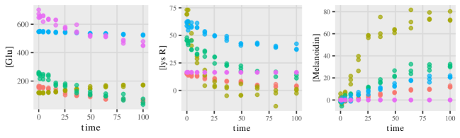
Figure 5: Sample observations (the method’s input) for the variables Glu, lys R and Melanoidin from Data Set 1. Points represent noisy observations with different colors for the $5$ different experimental conditions, e.g., red corresponds to experimental condition 1.

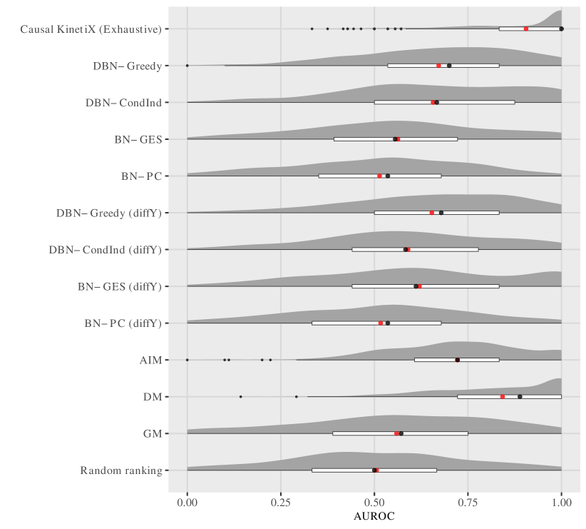
Figure 6: Results for simulation in Section D.2.1. In each of the $500$ simulations, the methods rank predictors for a randomly chosen target. If the AUROC equals one, the correct variables are ranked highest. Red points correspond to mean AUROC, black points to median AUROC.

D.2.2 Overfitting of the variable ranking

We now demonstrate that incorporating stability as a learning principle also helps in terms of overfitting. We again use data that were simulated according to Data Set 1. We compare CausalKinetiX with a modified version that does not hold out experiments in step (M4) of the procedure. This version therefore focuses on prediction and mostly neglects stability. We now compare the performance of the two procedures while increasing the number of terms in the model classes we search over. As can be seen from Figure 7 the decrease in AUROC is stronger for the method that focuses less on stability. We regard this as evidence that stability as an inference principle indeed helps against overfitting in these types of models (see also Section D.3.1).

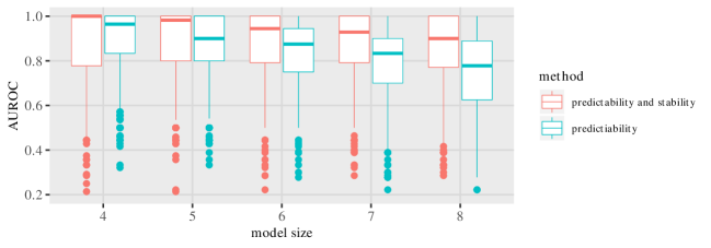
Figure 7: Results illustrating how CausalKinetiX behaves when model class is increased. Enforcing stability results in better regularization even on large model classes.

D.2.3 Effect of time-dependent measurement noise

The data simulated according to Data Set 1 is corrupted with time-independent measurement noise. However, we do not regard the assumption of i.i.d. measurement noise as crucial for our procedure: The noise becomes most relevant during the smoothing step of CausalKinetiX. As long as the distribution of the noise does not negatively impact the smoothing, the output of CausalKinetiX will be unaffected. Furthermore, even if there are biases induced in the smoother due to time-dependent noise, they do not necessarily harm CausalKinetiX as long as the dynamics are still captured to a satisfactory degree. This is why we expect CausalKinetiX to be robust with respect to time-dependent measurement noise. We verify this empirically by performing the same experiment as in Section D.2.1 but replacing the independent Gaussian noise with auto-regressive noise of the form

$$\varepsilon_{t}=a\cdot\varepsilon_{t-1}+W_{t},$$

where $a\in(-1,1)$ and $W_{t}$ is standard normal noise. (We furthermore screen down to $15$ terms to decrease the computation burden of the experiment.) The results for different values of $a$ are given in Figure 8 and illustrate that there is indeed no negative effect of time-dependent noise in this case.

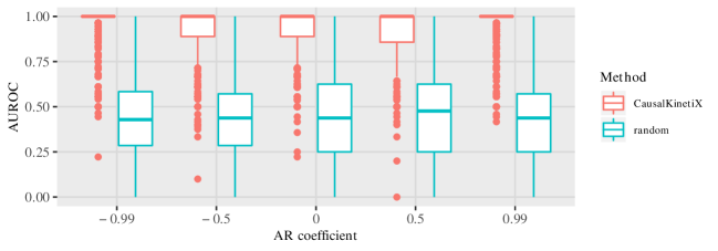
Figure 8: Results illustrating the affect of time-dependence in the measurement noise on the variable ranking performance of CausalKinetiX. Added time-dependence has no negative effect on the performance, which is expected since CausalKinetiX is based on dynamics rather than the trajectories directly.

D.2.4 Comparison of screening procedures

Using data generated as in Data Set 1, we compare the two screening methods based on GM and DM. To this end, we sample $B=1000$ data sets and apply both DM and GM to rank all $11\cdot 10\cdot 0.5+22=77$ individual terms of the form $X^{k}X^{j}$ and $X^{j}$ ($d=11$) based on their first entrance into the model. For each data set, we then compute the worst rank of any true term and plot them in Figure 9. For comparison, we also include the results from a random ranking, i.e., a random permutation of the terms. Both methods perform better than the random baseline, and DM outperforms GM in this setting. This might be because the integral approximation used in DM is more robust than the estimation of the derivatives required for GM.

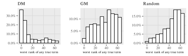
Figure 9: Comparison between different screening methods based on $B=1000$ simulations from Data Set 1 in Section D.2.1. All $77$ terms of the form $X^{k}X^{j}$ and $X^{j}$ are ranked according to the screening procedure. The x-axis shows the rank of the worst ranked term from the true model. High concentration on the left implies good screening performance. Here, DM outperforms GM.

D.2.5 Consistency analysis

We now illustrate our theoretical consistency result presented in the Methods section and Section B. Again, we simulate from Data Set 1, where we consider different values of $L$ and $n$ to analyze the asymptotic behavior. Instead of increasing the value of $n$ we decrease the noise variance as this has a similar effect but is computationally faster. Since computing the RankAccuracy requires knowledge of the invariant sets, we use a setting with many experimental conditions (here, $10$ experimental conditions) and assume that in this limit only super-sets of the true model are invariant. The results shown in Figure 10 demonstrate the convergence of the RankAccuracy towards one as the number of time steps $L$ goes to infinity and the noise variance goes to zero.

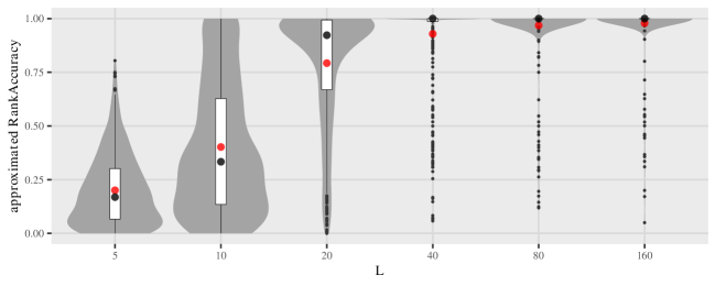
Figure 10: Results for simulation in Section D.2.5. For different numbers of time points $L$ and noise variance proportional $\frac{10}{L^{2}}$ we sampled $500$ simulations from Data Set 1. For each simulation we compute the $\operatorname{RankAccuracy}$. Red points correspond to mean $\operatorname{RankAccuracy}$, large black points to median $\operatorname{RankAccuracy}$.

D.2.6 Increasing experimental conditions

In this section, we illustrate how an increase in experimental conditions affects the variable ranking performance of CausalKinetiX. Again, we simulate from Data Set 1, where we consider different numbers of experimental conditions. To ensure the comparison is fair, we choose the number of repetitions per experimental condition to ensure that the number of total observations is fixed at 16. Furthermore, in order to remove any effect resulting from ordering of the variables we relabel them in each repetition by randomly permuting the labels. Each ranking is then assessed by computing the area under the operator receiver curve (AUROC) based on the known ground truth (i.e., parents of the target ${\mathbf{PA}}_{Y}$). The results are given in Figure 11. Here, we applied CausalKinetiX using the exhaustive model class (see B Section B.2) and considered all possible models consisting of individual variables and interactions ($66$ potential predictor terms). We restricted the search to models with at most $4$ such terms after reducing the number of terms by a prior screening step to $11$. The results show that CausalKinetiX benefits from an increased number of experimental conditions.

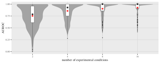
Figure 11: Results for simulation in Section D.2.6. For different numbers of experimental conditions we sampled $500$ simulations from Data Set 1. For each simulation we compute the AUROC. Red points correspond to mean AUROC, large black points to median AUROC.

D.2.7 Scalability

Next, we analyze how our method scales with the number of variables $d$, the number of environments $m$, the number of repetitions in each environment $R$, and the number of observed time points for each trajectory $L$. Figure 12 illustrates the run-time of our method when one of these parameters is varied while the others are kept fixed. The data are generated according to Data Set 2. The key steps driving the computational cost of our procedure are the smoothing in steps (M3) and (M5), as well as the estimation step (M4). In our case, the cost of the estimation procedure, fitting a linear model with ordinary least squares, is negligible. Since the number of smoothing operations, we have to perform grows linearly with respect to $m$ and $R$, we expect a linear increase in run-time. Accordingly, the slopes in Figure 12 (bottom left and top right) are close to one.

We compute the smoothing spline in (M3) using a convex quadratic program, which can be solved in polynomial time – even if the number of constraints grows linearly, see (M5). The data points in Figure 12 (bottom right) do not lie on a straight line, which may be due to some computational overhead for small values of $L$ or due to the quadratic program itself. The worst case complexity of convex quadratic programming is cubic in sample size, but many instances can be solved more efficiently. Correspondingly, the slope in Figure 12 (bottom right) is not larger than three. When only values $L\geq 64$ are taken into account, the slope is estimated as $2.9$, which is close to the worst case guarantee of $3$. Finally, varying the number of variables impacts the size of $\mathcal{M}$, that is, the number of models. In Figure 12, we consider the case of main-effects models of up to three variables, which results in $\mathcal{O}(d^{3})$ models. If we again assume that run-time of the estimation step can be neglected, we expect a slope of $3$ in the log-log plot. In our empirical experiments the slope is estimated as $2.8$ (Figure 12 top left).

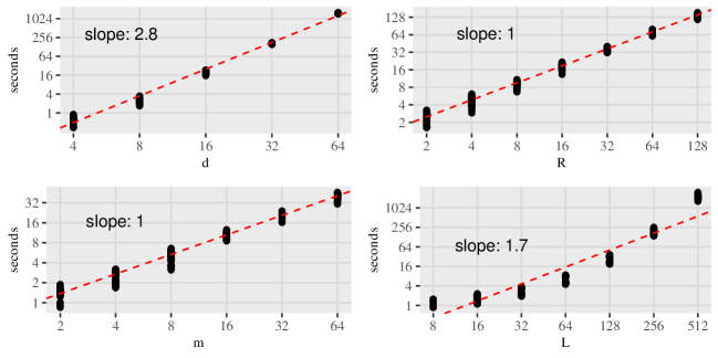
Figure 12: Run-time analysis for the parameters number of variables $d$, number of repetitions $R$, number of environments $m$ and number of time points $L$. In each plot one parameter is varied while the remaining are kept constant and the run-time is computed $100$ times for a full application of our method. The dotted red line is a linear fit to the log-log-transformed plots where the slope estimates the polynomial runtime order.

D.2.8 Allowing for complex predictor models

Our procedure requires that only the dynamics of the target variable are given by an ODE model. We do not model the dynamics of the predictors, which as a consequence may follow any arbitrarily complex model. As an illustration we sample trajectories such that the predictors are completely random and only the target variable satisfies an invariant model. The details of the data generation are shown in Data Set 2.

Consider functions of the form $$f_{c_{1},c_{2},c_{3},c_{4}}(t)=\frac{c_{1}}{1+e^{c_{2}(t-3)}}+\frac{c_{3}}{1+e^{c_{4}(t-3)}},$$ i.e., these functions are linear combinations of sigmoids which have smooth trajectories that imitate dynamics observed in some real data experiment. For each of the $5$ experimental conditions we sample $d=12$ trajectories $X_{t}^{j}=f_{c_{1},c_{2},c_{3},c_{4}}(t)$ for $t\in[0,6]$, where $c_{1},c_{2},c_{3},c_{4}$ are i.i.d. standard normal. Based on these trajectories and the ODE given by $$\dot{Y}_{t}=\theta_{1}X^{1}+\theta_{2}X^{2},\quad Y_{0}=0,$$ where $\theta_{1}=0.0001$ and $\theta_{2}=0.0002$, we compute the trajectories of the target variable $Y$ by numerical integration. Finally, the observations are given as noisy versions of the values of these trajectories on an equally spaced time grid with $L=15$ time points between $0$ and $10$. The noise at each observation is independently normal distributed with mean $0$ and variance proportional to the total variation norm of the trajectory plus a small positive constant (in case the trajectory is constant), i.e., $\sigma=c\cdot\lVert y\rVert_{\operatorname{TV}}+10^{-7}$, where $y(t)$ are the true trajectories and $c\sim\operatorname{Unif}(0.05,0.15)$. Sample trajectories are given in Figure 13.

The results are shown in Figure 14. Here, we applied CausalKinetiX for both the exhaustive and main effects model class. For the exhaustive model class we again consider individual variables and interactions as possible terms ($78$ terms) and reduce to half these ($39$ terms) using screening and then apply our method for all models with at most $3$ terms. For the main effect models we perform no screening and consider all models consisting of at most $3$ variables. Even though none of the predictors follows an ODE model our procedure is capable of recovering the true causal parents and again improves on plain prediction (DM and GM).

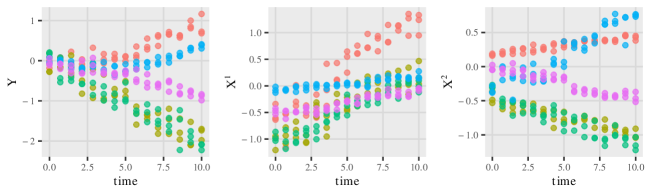
Figure 13: Sample observations for the target variable $Y$ and its two parents $X^{1}$ and $X^{2}$ Data Set 2. Points represent noisy observations with different colors used for the $5$ different experiments, e.g., red corresponds to experimental condition 1.

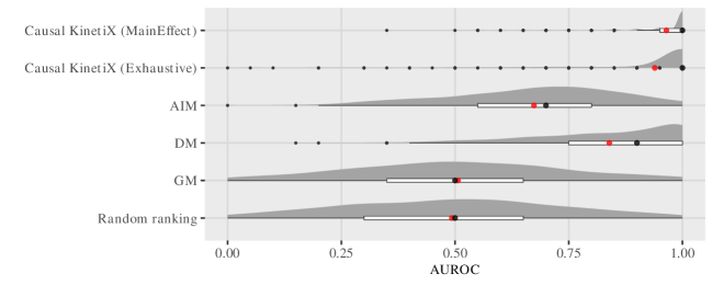
Figure 14: Results for simulation in Section D.2.8. Red points correspond to mean AUROC, large black points to median AUROC.

D.2.9 Robustness in the presence of hidden variables

In many practical applications hidden (unobserved) variables are omnipresent. Since we only model the target equation, hidden variables do not affect our methodology if they appear anywhere outside the target variable $Y$. In this section, we show that even if they enter the target equation our procedure is generally expected to behave well. The data in this section are generated according to Data Set 3, which is based on an artificially constructed ODE system, for which some of the variables are assumed to be hidden. Example trajectories are shown in Figure 15.

The exact ODE structure is given in Section D.4.2. We generate data from $16$ experimental conditions and sample $3$ repetitions for each experiment. The experimental conditions are the following. • Experimental condition $1$ (observational data):
Trajectories are simulated using the parameters given in Section D.4.2. • Experimental conditions $2$ to $16$ (interventional data):
Trajectories are simulated based on the following two types of interventions – initial value intervention: Initial values are sampled for $X^{1}$, $X^{2}$ and $X^{5}$ uniform between $0$ and $10$, the remainder of the quantities are kept at zero initially as they are all products of the reactions. – blocking reactions: Random reactions other than $k_{4}$, $k_{5}$ and $k_{7}$ are set to zero by fixing the corresponding reaction constant $k_{i}\equiv 0$. The expected number of reactions set to zero is $2$. Additionally, the rate $k_{7}$ is randomly perturbed either by sampling it uniform on $[0,0.2]$ or uniform on $[-0.1,0.3]$. Based on these experimental conditions each true trajectory is computed using numerical integration. Finally, the observations are noisy versions of the values of these trajectories on an exponential time grid with $L=20$ time points between $0$ and $100$. The noise at each observation is independently normal distributed with mean $0$ and variance proportional to the total variation norm of the trajectory plus a small positive constant (in case the trajectory is constant), i.e., $\sigma=c\cdot\lVert y\rVert_{\operatorname{TV}}+10^{-7}$, where $y(t)$ are the true trajectories and $c\sim\operatorname{Unif}(0.01,0.1)$. Example trajectories for the variables $X^{2}$ and $H^{2}$ depending on the values of $k_{7}$ are illustrated in Figure 15.

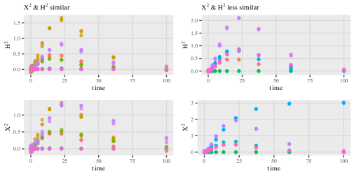
Figure 15: Sample observations of the two predictors $X^{2}$ and $H^{2}$ from Data Set 3 (only first $8$ experiments) for two different choices of perturbations of $k_{7}$. From left to right: For $k_{7}$ uniform on $[0,0.2]$ the dynamics are similar but not identical, for $k_{7}$ uniform on $[-0.1,0.3]$ the dynamics become very different. Points represent noisy observations of the underlying ODE trajectories.

We conduct three experiments, whose results are shown in Figure 16 and Figure 17. In the first setting (left plots), all variables are observed. The system of equations is built such that $X^{2}$ and $H^{2}$ obey very similar but not identical trajectories (here $k_{7}$ is perturbed less). Most methods are able to correctly identify $X^{3}$ and $H^{2}$ as the direct causes of $Y$ – those variables are usually ranked highest, see Figures 16 and 17 (left). In the second setting (middle plots), $H^{2}$ is unobserved. Because of the similarity between $H^{2}$ and $X^{2}$, the methods now infer $X^{2}$ as a direct cause. Finally, the third setting (right plots) differ from the second setting in the sense that $H^{2}$ and $X^{2}$ are significantly different (here $k_{7}$ is perturbed more). The latter variable still helps for prediction but does not yield an invariant model. CausalKinetiX still reliably infers $X^{3}$ as a direct cause, which is usually ranked higher than any of the other variables, see Figures 16 and 17 (right). The results show that CausalKinetiX is relatively robust against the existence of unobserved variables.

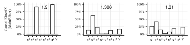
Figure 16: Results for the experiment described in Section D.2.9 (hidden variables). Plot shows how often each variable gets a $p$-value smaller than $0.01$. The number on each histogram is the average number of significant variables at a $1\%$ level.

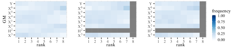
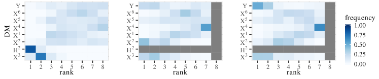
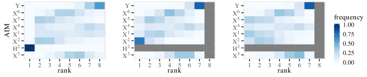
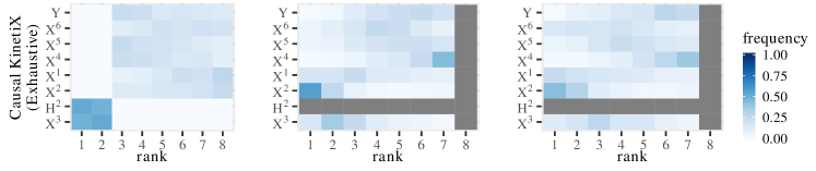
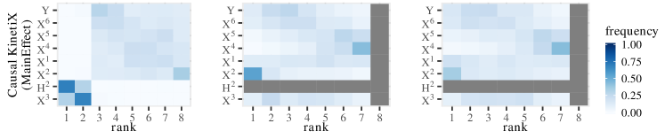
Figure 17: Results for the experiment described in Section D.2.9 (hidden variables). Left: all variables are observed. From top to bottom: Random, GM, DM, AIM, CausalKinetiX (Exhaustive), CausalKinetiX (Main Effect)

D.3 Supplementary results to metabolic networks analysis

The resulting integrated model fits when the entire model search procedure is performed by holding out one experiment is given in Figure 18. Despite the lack of heterogeneity in two of these held-out experiments, the CausalKinetiX variable ranking is very robust. To show this we look at the variable rankings of the fully-out-of-sample experiments from Figure 18. The results are presented in the table below. The true causal variables, as well as the true causal model, are unknown. For illustration purposes, we indicate which of the highly ranked variables appear in the model from above which has obtained the best score when based on all five experiments. (This model was able to explain all the variation in the different experiments, as illustrated by the plots in the main paper.) As a comparison, when screening down to only three terms one obtains the following different model

$$\dot{Y}_{t}=\theta_{1}Z_{t}X_{t}^{128}X_{t}^{128}+\theta_{2}Z_{t}X_{t}^{242}X_{t}^{298}-\theta_{3}Y_{t}X_{t}^{33}X_{t}^{138},$$

which are the terms included in DM-NONLSQ-3.

held-out-experiment rank 1 2 3 4 5 $\mathbf{1}$ $\mathbf{{\color[rgb]{0,0.390625,0}X^{33}}}$ $\mathbf{{\color[rgb]{0,0.390625,0}X^{33}}}$ $\mathbf{{\color[rgb]{0,0.390625,0}X^{33}}}$ $\mathbf{{\color[rgb]{0,0.390625,0}X^{33}}}$ $\mathbf{{\color[rgb]{0,0.390625,0}X^{33}}}$ $\mathbf{2}$ $\mathbf{{\color[rgb]{0,0.390625,0}X^{56}}}$ $X^{38}$ $X^{73}$ $X^{59}$ $\mathbf{{\color[rgb]{0,0.390625,0}X^{56}}}$ $\mathbf{3}$ $\mathbf{{\color[rgb]{0,0.390625,0}X^{122}}}$ $X^{61}$ $\mathbf{{\color[rgb]{0,0.390625,0}X^{122}}}$ $\mathbf{{\color[rgb]{0,0.390625,0}X^{128}}}$ $\mathbf{{\color[rgb]{0,0.390625,0}X^{122}}}$ $\mathbf{4}$ $\mathbf{{\color[rgb]{0,0.390625,0}X^{128}}}$ $\mathbf{{\color[rgb]{0,0.390625,0}X^{128}}}$ $\mathbf{{\color[rgb]{0,0.390625,0}X^{138}}}$ $\mathbf{{\color[rgb]{0,0.390625,0}X^{168}}}$ $\mathbf{{\color[rgb]{0,0.390625,0}X^{128}}}$ $\mathbf{5}$ $\mathbf{{\color[rgb]{0,0.390625,0}X^{138}}}$ $\mathbf{{\color[rgb]{0,0.390625,0}X^{138}}}$ $\mathbf{{\color[rgb]{0,0.390625,0}X^{168}}}$ $X^{246}$ $\mathbf{{\color[rgb]{0,0.390625,0}X^{138}}}$ $\mathbf{6}$ $\mathbf{{\color[rgb]{0,0.390625,0}X^{168}}}$ $\mathbf{{\color[rgb]{0,0.390625,0}X^{168}}}$ $X^{215}$ $X^{61}$ $\mathbf{{\color[rgb]{0,0.390625,0}X^{168}}}$ $\displaystyle\dot{Y}_{t}$ $\displaystyle=\theta_{1}Z_{t}\mathbf{{\color[rgb]{0,0.390625,0}X_{t}^{56}X_{t}^{122}}}$ $\displaystyle\quad+\theta_{2}Z_{t}\mathbf{{\color[rgb]{0,0.390625,0}X_{t}^{128}X_{t}^{168}}}$ $\displaystyle\quad-\theta_{3}Y_{t}\mathbf{{\color[rgb]{0,0.390625,0}X_{t}^{33}X_{t}^{138}}}$ (57)

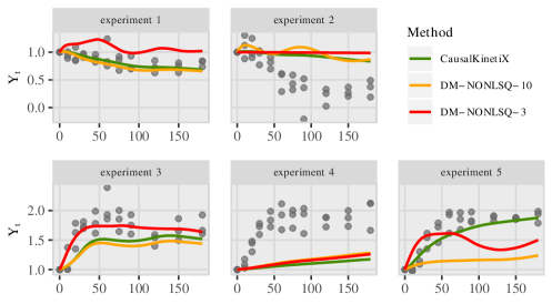
Figure 18: Metabolic network analysis. Fully out-of-sample fit. The plot shows the models’ ability to generalize to new experiments. Each plot shows model-based trajectories that are obtained when that experiment is neither used for model identification nor parameter estimation. This is a very hard problem. CausalKinetiX shows the best generalization performance.

D.3.1 Overfitting of trajectories in metabolic network

To underscore the findings in Section D.2.2, we further illustrate the regularizing effect of stability component of CausalKinetiX, we perform an additional experiment on the metabolic data. Starting from the model [57] we proceed by adding 5 terms (from the top $1000$ screened terms) in a greedy fashion based on two scores: (i) the standard CausalKinetiX score and (ii) the modified CausalKinetiX score which does not hold out experiments in step (M4) of the procedure. The results in Figure 19 highlight that stability is indeed helpful for regularizing the fitted trajectories.

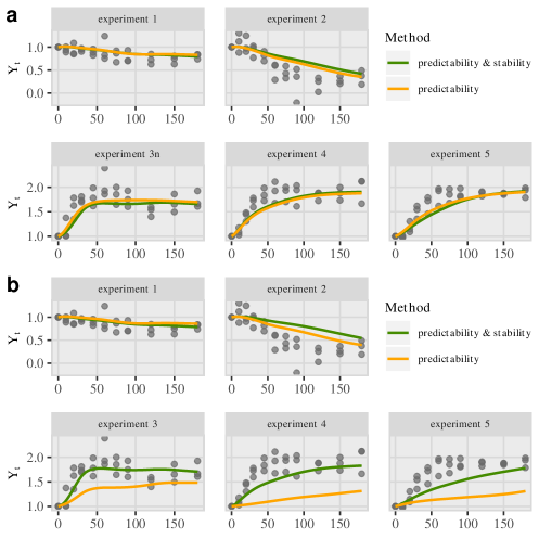
Figure 19: Stability as regularization to overfitting in metabolic network analysis. Comparison between two models consisting of 8 terms where each is constructed in a greedy fashion using a score measuring mainly predictability and our proposed score which includes stability. In a, the in-sample trajectories are shown and the model based solely on predictability performs better. In b, the out-of-experiment performance (same type of sample-splitting as in the main article Figure 4 b) of the same models are compared, illustrating the regularizing effect of including stability into the score.

D.4 Additional details on simulation settings

D.4.1 Biomodel 52

Glu $\displaystyle\overset{k_{1}}{\longrightarrow}\text{Fru}$ Fru $\displaystyle\overset{k_{2}}{\longrightarrow}\text{Glu}$ Glu $\displaystyle\overset{k_{3}}{\longrightarrow}\text{Formic acid}+\text{C5}$ Fru $\displaystyle\overset{k_{4}}{\longrightarrow}\text{Formic acid}+\text{C5}$ Fru $\displaystyle\overset{k_{5}}{\longrightarrow}2\cdot\text{Triose}$ Triose $\displaystyle\overset{k_{6}}{\longrightarrow}\text{Cn}+\text{Acetic acid}$ $\displaystyle\text{lys R}+\text{Glu}$ $\displaystyle\overset{k_{7}}{\longrightarrow}\text{Amadori}$ Amadori $\displaystyle\overset{k_{8}}{\longrightarrow}\text{Acetic acid}+\text{lys R}$ Amadori $\displaystyle\overset{k_{9}}{\longrightarrow}\text{AMP}$ $\displaystyle\text{lys R}+\text{Fru}$ $\displaystyle\overset{k_{10}}{\longrightarrow}\text{AMP}$ AMP $\displaystyle\overset{k_{11}}{\longrightarrow}\text{Melanoidin}$

$\displaystyle\tfrac{\text{d}}{\text{dt}}[\text{Glu}]$ $\displaystyle=-(k_{1}+k_{3})[\text{Glu}]+k_{2}[\text{Fru}]+k_{7}[\text{Glu}][\text{lys R}]$ $\displaystyle\tfrac{\text{d}}{\text{dt}}[\text{Fru}]$ $\displaystyle=k_{1}[\text{Glu}]-(k_{2}+k_{4}+k_{5})[\text{Fru}]-k_{10}[\text{Fru}][\text{lys R}]$ $\displaystyle\tfrac{\text{d}}{\text{dt}}[\text{Formic acid}]$ $\displaystyle=k_{3}[\text{Glu}]+k_{4}[\text{Fru}]$ $\displaystyle\tfrac{\text{d}}{\text{dt}}[\text{Triose}]$ $\displaystyle=2k_{5}[\text{Fru}]-k_{6}[\text{Triose}]$ $\displaystyle\tfrac{\text{d}}{\text{dt}}[\text{Acetic acid}]$ $\displaystyle=k_{6}[\text{Triose}]+k_{8}[\text{Amadori}]$ $\displaystyle\tfrac{\text{d}}{\text{dt}}[\text{Cn}]$ $\displaystyle=k_{6}[\text{Triose}]$ $\displaystyle\tfrac{\text{d}}{\text{dt}}[\text{Amadori}]$ $\displaystyle=-(k_{8}+k_{9})[\text{Amadori}]+k_{7}[\text{Glu}][\text{lys R}]$ $\displaystyle\tfrac{\text{d}}{\text{dt}}[\text{AMP}]$ $\displaystyle=k_{9}[\text{Amadori}]-k_{11}[\text{AMP}]+k_{10}[\text{Fru}][\text{lys R}]$ $\displaystyle\tfrac{\text{d}}{\text{dt}}[\text{C5}]$ $\displaystyle=k_{3}[\text{Glu}]+k_{4}[\text{Fru}]$ $\displaystyle\tfrac{\text{d}}{\text{dt}}[\text{lys R}]$ $\displaystyle=k_{8}[\text{Amadori}]-k_{7}[\text{Glu}][\text{lys R}]-k_{10}[\text{Fru}][\text{lys R}]$ $\displaystyle\tfrac{\text{d}}{\text{dt}}[\text{Melanoidin}]$ $\displaystyle=k_{11}[\text{AMP}]$

$\displaystyle k_{1}$ $\displaystyle=0.01$ $\displaystyle k_{2}$ $\displaystyle=0.00509$ $\displaystyle k_{3}$ $\displaystyle=0.00047$ $\displaystyle k_{4}$ $\displaystyle=0.0011$ $\displaystyle k_{5}$ $\displaystyle=0.00712$ $\displaystyle k_{6}$ $\displaystyle=0.00439$ $\displaystyle k_{7}$ $\displaystyle=0.00018$ $\displaystyle k_{8}$ $\displaystyle=0.11134$ $\displaystyle k_{9}$ $\displaystyle=0.14359$ $\displaystyle k_{10}$ $\displaystyle=0.00015$ $\displaystyle k_{11}$ $\displaystyle=0.12514$ $\displaystyle[\text{Glu}]\mid_{t=0}$ $\displaystyle=160$ $\displaystyle[\text{Fru}]\mid_{t=0}$ $\displaystyle=0$ $\displaystyle[\text{Formic acid}]\mid_{t=0}$ $\displaystyle=0$ $\displaystyle[\text{Triose}]\mid_{t=0}$ $\displaystyle=0$ $\displaystyle[\text{Acetic acid}]\mid_{t=0}$ $\displaystyle=0$ $\displaystyle[\text{Cn}]\mid_{t=0}$ $\displaystyle=0$ $\displaystyle[\text{Amadori}]\mid_{t=0}$ $\displaystyle=0$ $\displaystyle[\text{AMP}]\mid_{t=0}$ $\displaystyle=0$ $\displaystyle[\text{C5}]\mid_{t=0}$ $\displaystyle=0$ $\displaystyle[\text{lys R}]\mid_{t=0}$ $\displaystyle=15$ $\displaystyle[\text{Melanoidin}]\mid_{t=0}$ $\displaystyle=0$

D.4.2 Artificial hidden variable model

$\displaystyle X^{1}$ $\displaystyle\overset{k_{1}}{\longrightarrow}H^{1}$ $\displaystyle H^{1}$ $\displaystyle\overset{k_{2}}{\longrightarrow}X^{2}+H^{2}$ $\displaystyle H^{1}$ $\displaystyle\overset{k_{3}}{\longrightarrow}X^{1}$ $\displaystyle H^{2}$ $\displaystyle\overset{k_{4}}{\longrightarrow}Y$ $\displaystyle X^{3}$ $\displaystyle\overset{k_{5}}{\longrightarrow}Y+X^{4}$ $\displaystyle X^{1}+X^{4}$ $\displaystyle\overset{k_{6}}{\longrightarrow}X^{3}$ $\displaystyle X^{2}$ $\displaystyle\overset{k_{7}}{\longrightarrow}X^{6}$ $\displaystyle X^{5}$ $\displaystyle\overset{k_{8}}{\longrightarrow}X^{3}$ $\displaystyle X^{4}$ $\displaystyle\overset{k_{9}}{\longrightarrow}X^{5}$

$\displaystyle\tfrac{\text{d}}{\text{dt}}[X^{1}]$ $\displaystyle=-k_{1}[X^{1}]+k_{3}[H^{1}]-k_{6}[X^{1}][X^{4}]$ $\displaystyle\tfrac{\text{d}}{\text{dt}}[X^{2}]$ $\displaystyle=k_{2}[H^{1}]-k_{7}[X^{2}]$ $\displaystyle\tfrac{\text{d}}{\text{dt}}[X^{3}]$ $\displaystyle=-k_{5}[X^{3}]+k_{6}[X^{1}][X^{4}]+k_{8}[X^{5}]$ $\displaystyle\tfrac{\text{d}}{\text{dt}}[X^{4}]$ $\displaystyle=k_{5}[X^{3}]-k_{6}[X^{1}][X^{4}]-k_{9}[X^{4}]$ $\displaystyle\tfrac{\text{d}}{\text{dt}}[X^{5}]$ $\displaystyle=k_{9}[X^{4}]-k_{8}[X^{5}]$ $\displaystyle\tfrac{\text{d}}{\text{dt}}[X^{6}]$ $\displaystyle=k_{7}[X^{2}]$ $\displaystyle\tfrac{\text{d}}{\text{dt}}[H^{1}]$ $\displaystyle=k_{1}[X^{1}]-(k_{2}+k_{3})[H^{1}]$ $\displaystyle\tfrac{\text{d}}{\text{dt}}[H^{2}]$ $\displaystyle=k_{2}[H^{1}]-k_{4}[H^{2}]$ $\displaystyle\tfrac{\text{d}}{\text{dt}}[Y]$ $\displaystyle=k_{4}[H^{2}]+k_{5}[X^{3}]$

$\displaystyle k_{1}$ $\displaystyle=0.08$ $\displaystyle k_{2}$ $\displaystyle=0.08$ $\displaystyle k_{3}$ $\displaystyle=0.01$ $\displaystyle k_{4}$ $\displaystyle=0.1$ $\displaystyle k_{5}$ $\displaystyle=0.003$ $\displaystyle k_{6}$ $\displaystyle=0.06$ $\displaystyle k_{7}$ $\displaystyle=0.1$ $\displaystyle k_{8}$ $\displaystyle=0.02$ $\displaystyle k_{9}$ $\displaystyle=0.05$ $\displaystyle[X^{1}]\mid_{t=0}$ $\displaystyle=5$ $\displaystyle[X^{2}]\mid_{t=0}$ $\displaystyle=0$ $\displaystyle[X^{3}]\mid_{t=0}$ $\displaystyle=0$ $\displaystyle[X^{4}]\mid_{t=0}$ $\displaystyle=5$ $\displaystyle[X^{5}]\mid_{t=0}$ $\displaystyle=0$ $\displaystyle[X^{6}]\mid_{t=0}$ $\displaystyle=0$ $\displaystyle[H^{1}]\mid_{t=0}$ $\displaystyle=0$ $\displaystyle[H^{2}]\mid_{t=0}$ $\displaystyle=0$ $\displaystyle[Y]\mid_{t=0}$ $\displaystyle=0$

Figure 20: Graph representation of hidden variable ODE model. If the rate $k_{4}$ is equal to the rate $k_{7}$ the variables $X^{2}$ and $H^{2}$ will have identical dynamics.

References

• Aldrich [1989] J. Aldrich. Autonomy. Oxford Economic Papers, 41:15–34, 1989.
• Arteaga and Engelman [2014] C. L. Arteaga and J. A. Engelman. Erbb receptors: from oncogene discovery to basic science to mechanism-based cancer therapeutics. Cancer cell, 25(3):282–303, 2014.
• Bard [1974] Y. Bard. Nonlinear Parameter Estimation. Academic Press, New York, NY, 1974.
• Bareinboim and Pearl [2016] E. Bareinboim and J. Pearl. Causal inference and the data-fusion problem. Proceedings of the National Academy of Sciences, 113(27):7345–7352, 2016.
• Basu et al. [2018] S. Basu, K. Kumbier, J. B. Brown, and B. Yu. Iterative random forests to discover predictive and stable high-order interactions. Proceedings of the National Academy of Sciences, 115(8):1943–1948, 2018.
• Benson [1979] M. Benson. Parameter fitting in dynamic models. Ecological Modelling, 6:97–115, 1979.
• Blom and Mooij [2018] T. Blom and J. M. Mooij. Generalized structural causal models. arXiv preprint arXiv:1805.06539, 2018.
• Boninsegna et al. [2018] L. Boninsegna, F. Nüske, and C. Clementi. Sparse learning of stochastic dynamical equations. The Journal of Chemical Physics, 148(24):241723, 2018.
• Brands and van Boekel [2002] C. M. J. Brands and M. A. J. S. van Boekel. Kinetic modeling of reactions in heated monosaccharide-casein systems. Journal of agricultural and food chemistry, 50(23):6725–6739, 2002.
• Brunton et al. [2016] S. L. Brunton, J. L. Proctor, and J. N. Kutz. Discovering governing equations from data by sparse identification of nonlinear dynamical systems. Proceedings of the National Academy of Sciences, 113(15):3932–3937, 2016.
• Calderhead et al. [2009] B. Calderhead, M. Girolami, and N. D. Lawrence. Accelerating Bayesian inference over nonlinear differential equations with Gaussian processes. In Advances in neural information processing systems (NIPS), pages 217–224, 2009.
• Candès [2006] E. Candès. Compressive sampling. In Proceedings of the international congress of mathematicians, volume 3, pages 1433–1452. Madrid, Spain, 2006.
• Chen et al. [2017] S. Chen, A. Shojaie, and D. M. Witten. Network reconstruction from high-dimensional ordinary differential equations. Journal of the American Statistical Association, pages 1–11, 2017.
• Chen et al. [1999] T. Chen, H. He, and G. Church. Modeling gene expression with differential equations. In Biocomputing’99, pages 29–40. World Scientific, 1999.
• Chickering [2002] D. M. Chickering. Optimal structure identification with greedy search. Journal of Machine Learning Research, 3:507–554, 2002.
• Donoho [2006] D. Donoho. Compressed sensing. IEEE Transactions on information theory, 52(4):1289–1306, 2006.
• Eaton and Murphy [2007] D. Eaton and K. P. Murphy. Exact Bayesian structure learning from uncertain interventions. In Proceedings of the 11th International Conference on Artificial Intelligence and Statistics (AISTATS), pages 107–114, 2007.
• Fey et al. [2015] D. Fey, M. Halasz, D. Dreidax, S. P. Kennedy, J. F. Hastings, N. Rauch, A. G. Munoz, R. Pilkington, M. Fischer, F. Westermann, W. Koch, and B. N. Kholodenko. Signaling pathway models as biomarkers: Patient-specific simulations of jnk activity predict the survival of neuroblastoma patients. Sci. Signal., 8(408):ra130–ra130, 2015.
• Friston et al. [2003] K. Friston, L. Harrison, and W. Penny. Dynamic causal modelling. Neuroimage, 19(4):1273–1302, 2003.
• Haavelmo [1944] T. Haavelmo. The probability approach in econometrics. Econometrica, 12:S1–S115 (supplement), 1944.
• Hass et al. [2017] H. Hass, K. Masson, S. Wohlgemuth, V. Paragas, J. E. Allen, M. Sevecka, E. Pace, J. Timmer, J. Stelling, G. MacBeath, B. Schoeberl, and A. Raue. Predicting ligand-dependent tumors from multi-dimensional signaling features. NPJ Systems Biology and Applications, 3(1):27, 2017.
• Hindmarsh et al. [2005] A. C. Hindmarsh, P. N. Brown, K. E. Grant, S. L. Lee, R. Serban, D. E. Shumaker, and C. S. Woodward. SUNDIALS: Suite of nonlinear and differential/algebraic equation solvers. ACM Transactions on Mathematical Software, 31(3):363–396, 2005.
• Hoeting et al. [1999] J. Hoeting, D. Madigan, A. Raftery, and C. Volinsky. Bayesian model averaging: a tutorial. Statistical science, pages 382–401, 1999.
• Imbens and Rubin [2015] G. W. Imbens and D. B. Rubin. Causal Inference for Statistics, Social, and Biomedical Sciences: An Introduction. Cambridge University Press, New York, NY, 2015.
• Koller and Friedman [2009] D. Koller and N. Friedman. Probabilistic Graphical Models: Principles and Techniques. MIT Press, 2009.
• Li et al. [2010] C. Li, M. Donizelli, N. Rodriguez, H. Dharuri, L. Endler, V. Chelliah, L. Li, E. He, A. Henry, M. I. Stefan, J. L. Snoep, M. Hucka, N. Le Novère, and C. Laibe. Biomodels database: An enhanced, curated and annotated resource for published quantitative kinetic models. BMC systems biology, 4(1):92, 2010.
• Lim and Yu [2016] C. Lim and B. Yu. Estimation stability with cross-validation (ESCV). Journal of Computational and Graphical Statistics, 25(2):464–492, 2016.
• Maillard [1912] L. C. Maillard. Action des acides amines sur les sucres; formation des melanoidines par voie methodique. Comptes rendus de l’Académie des Sciences, 154:66–68, 1912.
• Meinshausen and Bühlmann [2010] N. Meinshausen and P. Bühlmann. Stability selection. Journal of the Royal Statistical Society: Series B, 72(4):417–473, 2010.
• Meinshausen et al. [2016] N. Meinshausen, A. Hauser, J. Mooij, J. Peters, P. Versteeg, and P. Bühlmann. Methods for causal inference from gene perturbation experiments and validation. Proceedings of the National Academy of Sciences, 113(27):7361–7368, 2016.
• Meyer [1966] P. Meyer. Probability and potentials. Blaisdell Publishing Company, 1966.
• Mikkelsen and Hansen [2017] F. V. Mikkelsen and N. R. Hansen. Learning large scale ordinary differential equation systems. arXiv preprint arXiv:1710.09308, 2017.
• Mooij et al. [2013] J. M. Mooij, D. Janzing, and B. Schölkopf. From ordinary differential equations to structural causal models: the deterministic case. In Proceedings of the 29th Conference Annual Conference on Uncertainty in Artificial Intelligence (UAI), pages 440–448, Corvallis, Oregon, USA, 2013. AUAI Press.
• Murray [2017] R. Murray. A mathematical introduction to robotic manipulation. CRC press, 2017.
• Oates et al. [2014] C. J. Oates, F. Dondelinger, N. Bayani, J. Korkola, J. W. Gray, and S. Mukherjee. Causal network inference using biochemical kinetics. Bioinformatics, 30(17):i468–i474, 2014.
• Ogunnaike and Ray [1994] B. Ogunnaike and W. Ray. Process dynamics, modeling, and control, volume 1. Oxford University Press New York, 1994.
• Pearl [2009] J. Pearl. Causality: Models, Reasoning, and Inference. Cambridge University Press, New York, USA, 2nd edition, 2009.
• Pearl and Mackenzie [2018] J. Pearl and D. Mackenzie. The Book of Why. Basic Books, New York, USA, 2018.
• Peters et al. [2016] J. Peters, P. Bühlmann, and N. Meinshausen. Causal inference using invariant prediction: identification and confidence intervals. Journal of the Royal Statistical Society, Series B (with discussion), 78(5):947–1012, 2016.
• Peters et al. [2017] J. Peters, D. Janzing, and B. Schölkopf. Elements of Causal Inference: Foundations and Learning Algorithms. MIT Press, Cambridge, MA, USA, 2017.
• Ramsay and Silverman [2005] J. O. Ramsay and B. W. Silverman. Functional Data Analysis. Springer, New York, NY, 2005.
• Ramsay et al. [2007] J. O. Ramsay, G. Hooker, D. Campbell, and J. Cao. Parameter estimation for differential equations: a generalized smoothing approach. Journal of the Royal Statistical Society: Series B (Statistical Methodology), 69(5):741–796, 2007.
• Raue et al. [2015] A. Raue, B. Steiert, M. Schelker, C. Kreutz, T. Maiwald, H. Hass, J. Vanlier, C. Tönsing, L. Adlung, R. Engesser, W. Mader, T. Heinemann, J. Hasenauer, M. Schilling, T. Höfer, E. Klipp, F. Theis, U. Klingmüller, B. Schöberl, and J. Timmer. Data2dynamics: a modeling environment tailored to parameter estimation in dynamical systems. Bioinformatics, 31(21):3558–3560, 2015.
• Regev et al. [2017] A. Regev, S. Teichmann, E. Lander, I. Amit, C. Benoist, E. Birney, B. Bodenmiller, P. Campbell, P. Carninci, M. Clatworthy, H. Clevers, B. Deplancke, I. Dunham, J. Eberwine, R. Eils, W. Enard, A. Farmer, L. Fugger, B. Göttgens, N. Hacohen, M. Haniffa, M. Hemberg, S. Kim, P. Klenerman, A. Kriegstein, E. Lein, S. Linnarsson, E. Lundberg, J. Lundberg, P. Majumder, J. Marioni, M. Merad, M. Mhlanga, M. Nawijn, M. Netea, G. Nolan, D. Pe’er, A. Phillipakis, C. Ponting, S. Quake, W. Reik, O. Rozenblatt-Rosen, J. Sanes, R. Satija, T. Schumacher, A. Shalek, E. Shapiro, P. Sharma, J. Shin, O. Stegle, M. Stratton, M. Stubbington, F. Theis, M. Uhlen, A. van Oudenaarden, A. Wagner, F. Watt, J. Weissman, B. Wold, R. Xavier, N. Yosef, and Human Cell Atlas Meeting participants. Science forum: the human cell atlas. Elife, 6:e27041, 2017.
• Ren et al. [2003] S-X. Ren, G. Fu, X-G. Jiang, R. Zeng, Y-G. Miao, H. Xu, Y-X. Zhang, H. Xiong, G. Lu, L-F. Lu, H-Q. Jiang, J. Jia, Y-F. Tu, J-X. Jiang, W-Y. Gu, Y-Q. Zhang, Z. Cai, H-H. Sheng, H-F. Yin, Y. Zhang, G-F. Zhu, M. Wan, H-L. Huang, Z. Qian, S-Y. Wang, W. Ma, Z-J. Yao, Y. Shen, B-Q. Qiang, Q-C. Xia, X-K. Guo, A. Danchin, S. Girons, R. Somerville, Y-M. Wen, M-H. Shi, Z. Chen, J-G. Xu, and G-P. Zhao. Unique physiological and pathogenic features of leptospira interrogans revealed by whole-genome sequencing. Nature, 422(6934):888, 2003.
• Rozman et al. [2018] J. Rozman, B. Rathkolb, M. Oestereicher, C. Schütt, A. Ravindranath, S. Leuchtenberger, S. Sharma, M. Kistler, M. Willershäuser, R. Brommage, T. Meehan, J. Mason, H. Haselimashhadi, IMPC Consortium, T. Hough, A-M. Mallon, S. Wells, L. Santos, C. Lelliott, J. White, T. Sorg, M-F. Champy, L. Bower, C. Reynolds, A. Flenniken, S. Murray, L. Nutter, K. Svenson, D. West, G. Tocchini-Valentini, A. Beaudet, F. Bosch, R. Braun, M. Dobbie, X. Gao, Y. Herault, A. Moshiri, B. Moore, K. Lloyd, C. McKerlie, H. Masuya, N. Tanaka, P. Flicek, H. Parkinson, R. Sedlacek, J. Seong, C-K. Wang, M. Moore, S. Brown, M. Tschöp, W. Wurst, M. Klingenspor, E. Wolf, J. Beckers, F. Machicao, A. Peter, H. Staiger, H-U. Häring, H. Grallert, M. Campillos, H. Maier, H. Fuchs, V. Gailus-Durner, T. Werner, and M. Hrabe de Angelis. Identification of genetic elements in metabolism by high-throughput mouse phenotyping. Nature communications, 9(1):288, 2018.
• Rubenstein et al. [2018] P. Rubenstein, S. Bongers, J. M. Mooij, and B. Schölkopf. From deterministic ODEs to dynamic structural causal models. In Proceedings of the 34th Conference Annual Conference on Uncertainty in Artificial Intelligence (UAI), Corvallis, Oregon, USA, 2018. AUAI Press.
• Rudy et al. [2017] S. H. Rudy, S. L. Brunton, J. L. Proctor, and J. N. Kutz. Data-driven discovery of partial differential equations. Science Advances, 3(4):e1602614, 2017.
• Schaeffer [2017] H. Schaeffer. Learning partial differential equations via data discovery and sparse optimization. Proceedings of the Royal Society A, 473(2197):20160446, 2017.
• Schölkopf et al. [2012] B. Schölkopf, D. Janzing, J. Peters, E. Sgouritsa, K. Zhang, and J. M. Mooij. On causal and anticausal learning. In Proceedings of the 29th International Conference on Machine Learning (ICML), 2012.
• Scutari and Denis [2014] M. Scutari and J.-B. Denis. Bayesian Networks with Examples in R. Chapman and Hall, Boca Raton, 2014. ISBN 978-1-4822-2558-7, 978-1-4822-2560-0.
• Shampine [2018] L. F. Shampine. Numerical solution of ordinary differential equations. Routledge, 2018.
• Shiffrin [2016] R. M. Shiffrin. Drawing causal inference from big data. Proceedings of the National Academy of Sciences, 113(27):7308–7309, 2016.
• Spirtes et al. [2000] P. Spirtes, C. Glymour, and R. Scheines. Causation, Prediction, and Search. MIT Press, 2nd edition, 2000.
• Szederkényi et al. [2011] G. Szederkényi, J. R. Banga, and A. A. Alonso. Inference of complex biological networks: distinguishability issues and optimization-based solutions. BMC systems biology, 5(1):177, 2011.
• Tibshirani [1994] R. Tibshirani. Regression shrinkage and selection via the lasso. Journal of the Royal Statistical Society, Series B, 58:267–288, 1994.
• Tibshirani et al. [2015] R. Tibshirani, M. Wainwright, and T. Hastie. Statistical learning with sparsity: the lasso and generalizations. Chapman and Hall, 2015.
• Tran and Ward [2017] G. Tran and R. Ward. Exact recovery of chaotic systems from highly corrupted data. Multiscale Modeling & Simulation, 15(3):1108–1129, 2017.
• Wu et al. [2014] H. Wu, T. Lu, H. Xue, and H. Liang. Sparse additive ordinary differential equations for dynamic gene regulatory network modeling. Journal of the American Statistical Association, 109(506):700–716, 2014.
• Yu [2013] B. Yu. Stability. Bernoulli, 19(4):1484–1500, 2013.
• Yu and Kumbier [2019] B. Yu and K. Kumbier. Three principles of data science: predictability, computability, and stability (pcs). arXiv preprint arXiv:1901.08152, 2019.
• Zhang [2005] W-B. Zhang. Differential equations, bifurcations, and chaos in economics, volume 68. World Scientific Publishing Company, 2005.