The persistent homology of a sampled map
Abstract
This paper aims to introduce a filtration analysis of sampled maps based on persistent homology, providing a new method for reconstructing the underlying maps. The key idea is to extend the definition of homology induced maps of correspondences using the framework of quiver representations. Our definition of homology induced maps is given by most persistent direct summands of representations, and the direct summands uniquely determine a persistent homology. We provide stability theorems of this process and show that the output persistent homology of the sampled map is the same as that of the underlying map if the sample is dense enough. Compared to existing methods using eigenspace functors, our filtration analysis has an advantage that no prior information on the eigenvalues of the underlying map is required. Some numerical examples are given to illustrate the effectiveness of our method.
1 Introduction
Consider the following problem.
Problem 1.1.
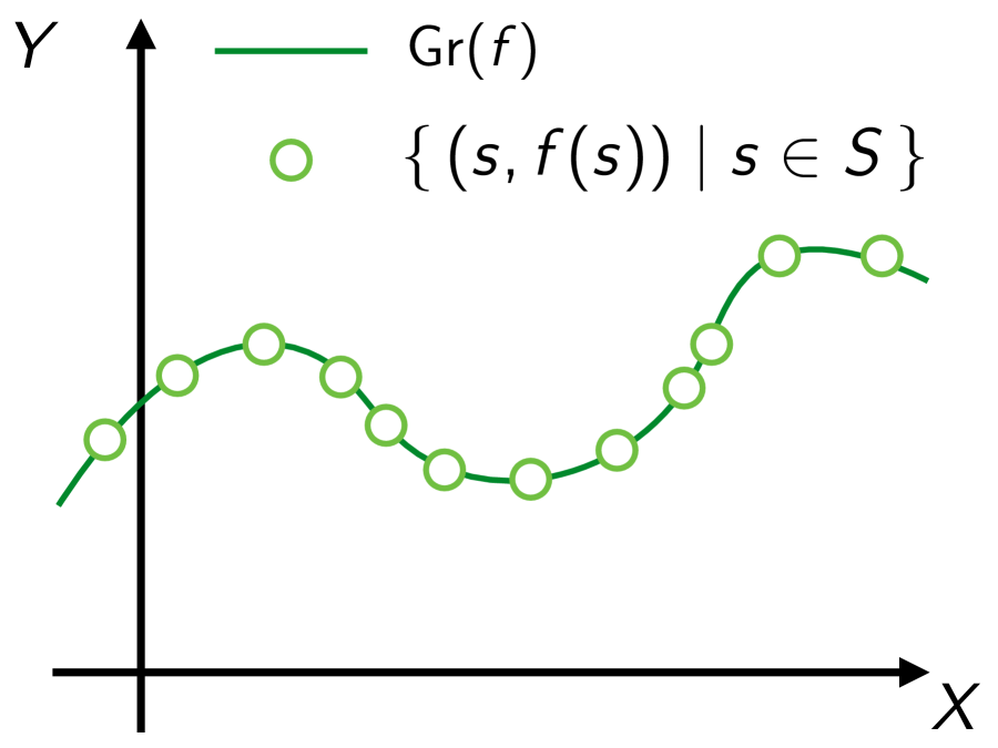
Let and be topological spaces, and be a continuous map. If we know only , , and sampling data , which is a restriction of on a finite subset , then can we retrieve any information about the homology induced map ?
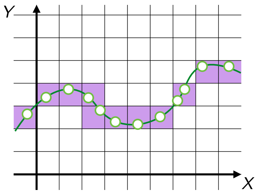
The map is called a sampled map of . This paper is motivated by [Harker et al. 2016], which suggests the following analysis for sampled maps. A grid of is a finite collection of subsets of with disjoint interiors such that . First, we divide the topological spaces and into grids and , and let be the union of regions which have elements of the sample . That is,
| (1) |
the purple regions in Figure 2. The set is an approximation of the graph from the sampled map by this subspace, which is called a correspondence.
Definition 1.2.
A correspondence from to is a subspace of .
Definition 1.3.
For a correspondence , let and be canonical projections, and and be their homology induced maps. If and satisfy two properties
-
•
(homologically complete)
-
•
(homologically consistent),
then the induced map of is defined by , and is well-defined.
The graph of is a correspondence. Since is continuous, is homeomorphic. As a consequence, and for satisfy homologically completeness and homologically consistency, hence is well-defined. We remark that this induced map coincides with . The following theorem guarantees that restores when the grid is fine and the sample is dense enough.
Theorem 1.4 ([Harker et al. 2016, Theorem 3.10]).
If a correspondence satisfies and is homologically consistent, then is well-defined and .
In Section 3, we give a new definition of induced maps of correspondences within the framework of quiver representations. We will see that the indecomposable decompositions of quiver representations give us an assignment among the bases of , , and , which defines the induced map from to .
The paper [Edelsbrunner et al. 2015] gives a way to analyze the eigenspaces of the homology induced map of a self-map (discrete dynamical system). In this analysis, the authors construct a filtration of simplicial maps from the sampled map and build its persistent homology by applying the homology functor and eigenspace functors. This construction of the filtration and the new definition of homology induced maps provide a further technique that enables another persistence analysis of sampled maps, shown in Section 4. Specifically, the assignment among the bases can compress the three persistent homologies generated by the finite sets , , and , yielding a persistent homology which describes the persistence of the topological mapping from the domain to the image of the induced map . Moreover, we can provide such a persistence analysis also in the above gridded setting, as mentioned in Subsection 4.2.
The main theorem of this paper is a stability theorem for these processes, Theorems 5.4 and 5.6 in Section 5, which state that these mappings from the input (sampled maps) to output (persistent homology or persistence diagrams) are non-expanding maps.
2 Preliminaries
In this section, we introduce quiver representations and matrix notation for morphisms between type representations. For more details, the reader can refer to [Assem et al. 2006] and [Asashiba et al. 2019], respectively.
2.1 Quivers and their representations
Throughout this paper, scalars of vector spaces and coefficient rings of homology groups are a fixed field . A quiver (or simply ) is a directed graph with a set of vertices , a set of arrows , and morphisms identifying the source and the target vertex of an arrow. An arrow is denoted by . A representation of a quiver , denoted (or simply or ), is a collection of a (finite dimensional) vector space for each vertex and a linear map for each arrow .
A morphism from to is defined by
| (2) |
with commutativity
| (3) |
The composition of morphisms and is .
These definitions determine an additive category of representations . Specifically, has a zero representation, isomorphisms of representations, and direct sums of representations. One can see the concrete construction of these in [Assem et al. 2006].
A representation is indecomposable if implies or . From the Krull-Remak-Schmidt theorem, every representation can be uniquely decomposed into a direct sum of indecomposables , unique up to isomorphism and permutations.
A quiver is of finite type if the number of distinct isomorphism classes of indecomposables is finite, and is of infinite type otherwise.
type quivers (or simply type quivers) are a class of quivers with the following shape:
| (4) |
where denotes a forward arrow or backward arrow , and is a sequence of symbols and which determine the orientation of the arrows. From Gabriel’s theorem [Gabriel 1972], every type representation
| (5) |
can be uniquely decomposed into a direct sum of indecomposable interval representations
| (6) | ||||
| (7) |
In topological data analysis, a central role is played by persistent homology. The homology of a filtration of simplicial complexes
| (8) |
can be regarded as a representation of an type quiver in the framework of quiver representations. Each interval representation corresponds to a generator of a homology group which is born at and dies at , and is called its lifetime. The persistence diagram is a multiset determined by the unique decomposition of the persistent homology
| (9) |
or an image made by plotting this on a plane. This description allows us to overview the generators of all homology groups, and hence this approach is frequently used for the application of persistent homology.
The framework of quiver representations has extended persistent homology to general representations of quivers. We call representations of quivers persistence modules. Zigzag persistence modules [Carlsson and de Silva 2010] are a typical example of the extension, which enable persistence analysis of time series data.
Consider deformations of topological spaces , a sequence of topological spaces. The zigzag persistence of the sequence is the representation of an type quiver
| (10) |
composed by the unions of neighboring spaces and their canonical inclusions. The decomposition of the zigzag persistence module as a representation yields a persistence diagram again, where each interval captures the persistence of a homology generator in the deformations of spaces.
2.2 Matrix notation for morphisms in
The paper [Asashiba et al. 2019] established a new matrix notation for morphisms in in the following way. This notation will give a clear perspective when arguing the well-definedness of persistence analysis in Section 4.
Definition 2.1 ([Asashiba et al. 2019, Definition 3]).
The arrow category of the category is a category whose objects are all morphisms in , where morphisms are defined as follows. For two objects and in this category, an morphism from to is a pair of morphisms and satisfying . The composition of morphisms and is defined by .
We remark that every morphism between representations of is isomorphic to a morphism between direct sums of interval representations
| (11) |
in , where
| (12) |
are indecomposable decompositions. By the following lemma, the morphism can be written down in a matrix form.
Definition 2.2 ([Asashiba et al. 2019, Definition 4]).
The relation is defined on the set of interval representations of , , by setting if and only if is nonzero. We write if and .
Lemma 2.3 ([Asashiba et al. 2019, Lemma 1]).
Let and be interval representations of .
-
1.
The dimension of as a -vector space is either 0 or 1.
-
2.
A -vector space basis can be chosen for each such that if , and , then
(13)
We use the notation over . A candidate for the basis is
| (14) |
in the case that . In the case that , we define for convenience. We fix this basis throughout this paper.
The morphism can be written in block matrix form
| (15) |
where each is composition of the canonical inclusion with the canonical projection :
| (16) |
In a similar way, each block can also be written in matrix form with the entries in :
| (17) |
For each relation , according to Lemma 2.3 and factoring out from each , we can get for some . In a similar way, factoring out from each , we get
| (18) |
where each is a matrix with the entries in .
Definition 2.4.
Let be a morphism in . The block matrix form of is
| (19) |
The paper [Asashiba et al. 2019] shows that isomorphisms in the arrow category correspond to row and column operations in block matrix form. These operations are performed by matrix multiplication with the same restriction, that is, the block of must be always zero. The column and row operations are almost the same as that of -matrices, however because of the restriction, addition from a block to certain blocks is not permissible.
Let us discuss column operations. We define a morphism such that the following diagram commutes:
| (20) |
where is an isomorphism. Namely, and are isomorphic in the arrow category. The morphism is also a morphism between direct sums of interval representations, hence in the same way, can also be written in block matrix form . The multiplication denotes column operations on , and its block at column and row is
| (21) | ||||
| (22) |
The difference from the usual column operations on -matrices is the part of not only the morphism but also the summation . The existence of the morphism just means that the block with must always be zero even when added from the other part. The summation might be a bit more complicated. It means that not all of the column operations are permissible, but only the following cases.
-
•
Elementary column operations (switching, multiplication, and addition) within the same interval is always permissible.
-
•
Column addition to from another interval with relation is permissible.
Similar properties of permissibility hold for row operations.
-
•
Elementary row operations (switching, multiplication, and addition) within the same interval is always permissible.
-
•
Row addition to from another interval with relation is permissible.
The following is an example of permissibility in the case of .
Example 2.5.
The following matrix is the block matrix form of , where we use the symbols to denote the rows and columns corresponding to the direct summands . Each block is abbreviated to if and otherwise. The prohibited additions for columns and rows, written as red arrows, correspond to the positions of the zero blocks . Since column addition from lower to upper blocks and row addition from left to right blocks are always prohibited, we write down only the prohibited column additions from upper to lower, and prohibited row addition from right to left. A notable fact is that either or is 0 for arbitrary . In other words, if and only if . We will refer to this fact in the proof of Lemma 4.3.
| (23) |
3 The induced maps via quiver representations
In this section, we redefine the induced map of a correspondence by using quiver representations. Let be the homology functor with coefficient . As a representation of an type quiver, the diagram induced by a correspondence can be decomposed into a direct sum of interval representations:
| (24) |
This indecomposable decomposition can be written as the diagram
| (25) |
The choice of bases gives us a relationship between bases of and , which can be regarded as a map from to . For example, an interval representation assigns an element of the standard basis of to 0 in . Therefore, non-trivial assignment happens only on the interval representations . By regarding the other interval representations as maps from to , we can define a map factoring the interval
| (26) |
where the arrows are the canonical projections of the vector spaces, and the morphism is the canonical injection of the vector space. Composing the path of morphisms, we can define the induced map of through as
| (27) |
This definition does not need the two assumptions mentioned in Definition 1.3. Although our definition depends on the choice of isomorphism of indecomposable decomposition, when the two assumptions are satisfied, our definition coincides with the original definition by the following theorem.
Theorem 3.1.
Define . If is homologically complete and homologically consistent, then .
Proof.
The claim to prove is
| (28) |
Since the morphism is surjective, this is equivalent to
| (29) |
In addition, because of the homological consistency , hence what we should prove is
| (30) |
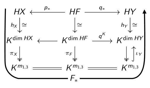
By chasing the diagram of Figure 3, this equation results in
| (31) |
The standard basis of corresponds to the standard bases of the four intervals , , , and . Here we remark that the homological consistency is equivalent to , namely does not exist as a direct summand. Moreover, the basis corresponding to and is mapped to by both and . By definition it is clear that holds for each element of the standard basis of corresponding to the standard bases of . ∎
4 Persistence analysis for sampled maps
The ability to decompose and focus exclusively on the interval representation provides persistence analysis for sampled maps. Let us consider the following problem, which is similar to Problem 1.1 but requires additional assumptions of embeddings.
Problem 4.1.
Let be a continuous map for . If , , and are unknown, and we know only a sampled map which is a restriction of on a finite subset , then can we retrieve any information about the homology induced map ?
Note that the sampling is a point cloud capturing topological features of when is dense enough. Originally the paper [Edelsbrunner et al. 2015] sets this problem with the more additional assumption that and constructs a persistent homology of eigenspaces of the sampled map, in order to analyze the eigenspaces of the discrete dynamical system .
In this section, we explain how to construct another persistent homology of a sampled map, which captures the generator of and connected by . We can utilize two types of filtrations in Subsections 4.1 and 4.2. The former filtration is generated using simplicial complexes, and we will prove a stability theorem (Theorem 5.4) of this construction in Section 5. The latter filtration is generated using grids as in Section 3, and also derives stability (Theorem 5.6). The stability theorem for the latter, however, requires more assumptions than for the former. Hence we explain in this order.
4.1 Construction using simplicial complexes
First, we generate a filtration of abstract simplicial complexes of ,
| (32) |
each simplex of which has elements of as its vertices, so that the filtration can capture the topology of the underlying space . For example, Čech complexes or Vietoris–Rips complexes [Edelsbrunner and Harer 2010] are available.
Definition 4.2.
Let be a finite set. The Čech complex for with a radius is an abstract simplicial complex defined as
| (33) |
where is the closed ball of center and radius . Let be the Euclidean metric on . The Vietoris–Rips complex for with a radius is an abstract simplicial complex defined as
| (34) |
Similarly, we also generate a filtration of abstract simplicial complexes
| (35) |
for .
Using these filtrations, we attempt to build a filtration of maps from to analyze the persistence of the original map , in analogy with the classical technique of persistent homology. Although we expect the sampled map to derive a simplicial map on each -th filter, in general, they can derive only a simplicial partial map111A correspondence from to is partial map if is a singleton or empty set for all , where . . Namely, for a simplex , it is not assumed that . Hence, the conventional technique computing topological persistence for simplicial maps [Dey et al. 2014] is not available in this setup.
We remark that the graph of the sampled map is a point cloud in . Let us define the -th abstract simplicial complex of as
| (36) |
One can show that forms a filtration. The sequence of the partial maps can be regarded as a sequence of pairs of canonical projections . This sequence of pairs constitutes a filtration induced by the inclusion maps of the filtration
| (37) |
Applying the homology functor to the sequence, we obtain a sequence of representations of the type quiver:
| (38) |
Remark 1.
The earlier research [Edelsbrunner et al. 2015] used domains of partial maps to construct a similar filtration. For a partial map 222To be accurate, the earlier research considers only the case that to analyze self-maps., the domain is defined as
| (39) |
Using the inclusion and the simplicial map induced by the map on , in a similar way the domains induce the representation
| (40) |
By the definitions of and , it is straightforward to see that the induced representation (40) is isomorphic to our representation (38). For the sake of consistency from the viewpoint of graphs and correspondences, we adopt the simplicial complexes .
Here, decomposing each filter as a representation to the intervals , the representation (38) is isomorphic to
| (41) |
Projecting to again, we obtain a sequence of subrepresentations
| (42) |
which is three copies of an type representation as we will see later.
We should be careful in the construction of . We write canonical projections and injections defined by direct sum as
| (43) | |||
| (44) |
respectively, and the morphisms in as
| (45) |
Then, the morphism in
| (46) |
is defined by
| (47) |
which is the submatrix at in block matrix form of .
At a glance, this construction seems natural, but “” is not a morphism in the representation category. Namely,
| (48) |
does not always commute. Consequently, the choice of isomorphism of indecomposable decomposition on each filter may make a difference in the output persistence diagram. In order to make sense of this analysis, the output persistence diagram should be uniquely determined and independent of the choice of isomorphism. The following theorem guarantees uniqueness and independence.
The restriction to the block has the following functoriality.
Lemma 4.3.
Let
| (49) |
and
| (50) |
be block matrix forms, then
| (51) |
Proof.
Let the corresponding scalar matrix symbols of and be and , respectively. The block matrix of at is
| (52) | ||||
| (53) |
but only can be the candidate for the interval as we saw in Example 2.5. Therefore
| (54) | ||||
| (55) | ||||
| (56) |
∎
Lemma 4.4.
Let be the block matrix form of an isomorphism, then is an isomorphism.
Proof.
Let be the inverse of . By Lemma 4.3,
| (57) |
and the left-hand side is the block of the identity map, which is the identity map on . Similarly, is identity map on , hence is isomorphic. ∎
Theorem 4.5.
The isomorphism class of
| (58) |
is uniquely determined and independent of the choice of the bases of
| (59) |
Proof.
Since regarding as omits no information, the sequence can be seen as a sequence of vector spaces
| (63) |
which is an type representation. We call this representation persistent homology of the sampled map . Decomposing into intervals, we can draw a persistence diagram, which shows us the robustness of the generators of homology in both filtrations, which are assigned by . Simultaneously we have constructed the filtration of complexes approximating the unknown spaces and .
In comparison with the earlier research
This persistence diagram does not provide any information about eigenvectors, unlike [Edelsbrunner et al. 2015]; however, it can be widely applied. First, since our method does not use the eigenspace functor, we need not require both sides’ spaces to be the same. Therefore, even in the case of sampled dynamical systems like the previous research, we can weaken the assumption to and take another filtration on . (If is not dense enough for sampling , then we can take instead.) Moreover, since the previous method needs to set an eigenvalue before analysis, they have to predict some behavior of in advance, but our method does not need any prior information. The numerical experiments in Section 7 will emphasize this difference.
4.2 Constriction using a grid
Subsequently, we provide another construction of a filtration constructed by dividing the spaces. Suppose the spaces and are embedded into Euclidean space , and both are divided by -dimensional -cubes
| (64) |
To distinguish the two divisions, we write this set as for the side Euclidean space and for side. Let be a sampled map of a continuous map , and and be the canonical projections of to the side and side Euclidean spaces, respectively. First, we generate a correspondence
| (65) |
where (see Figure 2).
In this setup, we use the metric for both spaces and . To construct a filtration along with the grids, let us define the filtration of a correspondence
| (66) |
and morphisms and . Here we restrict for sufficiently large . Then we have a similar diagram as before,
| (67) |
allowing us to obtain the filtrations and , capturing the persistent topological features of and . Again, the homology functor derives the sequence of morphisms in , therefore we can execute the same analysis as before, transforming it into block matrix form, restricting to the blocks , identifying it with a representation of the type quiver, and producing a persistence diagram.
5 Stability
In order for a tool in topological data analysis to be considered practical, the output persistence diagrams should behave continuously toward input data. Such a property is known as a stability theorem [Cohen-Steiner et al. 2007, Chazal et al. 2009] and has been proved for persistence modules on .
Let be the category of finite dimensional vector spaces, be the poset category of real numbers333For , a morphism uniquely exists if and only if .. An object of the functor category is also called a persistence module in some papers. To distinguish it from our definition, we call this an -persistence module.
Specifically, for an -persistence module , we assign a vector space for and a linear map for , where
| (68) |
for all . We call the linear maps transition maps. A morphism of -persistence modules is a natural transformation, that is a collection of morphisms commuting
| (69) |
for all .
We remark that every persistence module can be similarly regarded as a functor from a finite poset category to .
The fundamental objects of -persistence modules are interval modules for intervals , given by for and otherwise, and with the morphism corresponding to is an identity map. As is the case with persistent homology, every -persistence module can be decomposed into a direct sum of interval modules [Crawley-Boevey 2015].
We can define a distance between -persistence modules, called the interleaving distance.
Definition 5.1.
For , define the functor , called the shift functor, as follows. For an -persistence module , and . For a morphism in , .
Definition 5.2.
For an -persistence module and , the -transition morphism is defined as .
Definition 5.3.
-persistence modules and are said to be -interleaved if there exist morphisms and such that
| (70) |
The interleaving distance is defined by
| (71) |
An often used distance between persistence diagrams is the bottleneck distance, which is defined by bijections between them. It is well-known that the interleaving distance of -persistence modules is equal to the bottleneck distance of their persistence diagrams [Lesnick 2015, Bauer and Lesnick 2014]. Hence, by showing that a distance between input data is greater than the interleaving distance of their -persistence module, we can prove the stability of the persistence diagrams toward input data.
In analogy with [Edelsbrunner et al. 2015], stability theorems for some filtrations also hold on our analysis as follows. The discrete setting discussed in Section 4 is enough for implementation, but we extend it to a continuous analysis to prove its stability.
Now we use the following filtrations for and . Let be a distance on defined by
| (72) |
where is the Euclidean metric on . For a subset of , we define a function to be infimum distance to a point in . In the same way, we define the function for a subset of . We use the notation to denote the sublevel sets.
Let be the functor category from the type quiver as a poset category to the category of topological spaces. The sublevel sets , , and constitute the filtration in with morphisms induced by the inclusions such that the diagram
| (73) |
commutes for every .
In the same way as in the discrete analysis, applying the homology functor to the filtration produces , which is a family of objects in the representation category with the induced morphisms from Diagram (73).
Remark 2.
We have constructed the different representations from the previous representations using complexes in Subsection 4.1, but these are isomorphic if we adopt Čech complexes. It is known by the Nerve Lemma [Borsuk 1948] that, if is a finite subset in a metric space, then the sublevel set is homotopy equivalent to the Čech complex of with radius . Therefore, letting , , and be Čech complexes with radius of the finite subsets , , and , respectively, the induced family is isomorphic to the family .
Since decomposing every representation into intervals is isomorphic in the functor category , the family is isomorphic to , and the induced morphisms can be written in block matrix form again.
By Lemmas 4.3 and 4.5, the family and the induced morphisms are uniquely determined up to isomorphism. This gives us three copies of the -persistence module . Thus, we obtain an -persistence module . We denote this -persistence module of the sampled map as and call it the -persistence module of the sampled map.
Remark 3.
The construction of an -persistence module using graphs does not require the assumption that is a finite set. Therefore, if we assume that , , and are finite for an arbitrary , then the same analysis can be executed on the filtration , deriving an -persistence module in the same way. We call this the -persistence module of the map . The output persistence diagram portrays the robustness of the generators of the homology induced map .
After these setups, we can show the following stability theorem.
Theorem 5.4.
Let be a Hausdorff distance induced by . For two sampled maps and , let , be the -persistence modules of the sampled maps. Then,
| (74) |
Proof.
Let , and be an arbitrary real number.
By the definition of Hausdorff distance, and . Moreover, implies that and , hence , , , and as well. These inclusions induce the commutative diagrams:
| (75) |
and
| (76) |
By those functoriality, it is straightforward that these inclusions induce -interleaving morphisms between and , and we have . ∎
Accordingly, the obtained persistence modules and persistence diagrams can only have as much noise as or its evaluation by .
Since the proof does not use the assumption that is a finite set, a similar inequality holds for -persistence modules of maps.
Corollary 5.5.
Let and be subsets in . If -persistence modules and of maps and are defined, then
| (77) |
By Corollary 5.5, the error (bottleneck distance) between the persistence diagram of a sampled map and that of the original map is bounded by the error of the sampled map. If the sampled map is dense enough, we can infer the persistent generators of from the persistence module of the sampled map.
Finally, let us provide the stability of the persistence analysis using grids. We regard the persistent homology constructed using a grid as an -persistence module by the embedding induced by
| (78) |
Theorem 5.6.
Let be a Hausdorff distance induced by . For two sampled maps and , we write the filtrations of correspondences as and , and let and be their output -persistence modules. If , then .
Proof.
The assumption derives the inequality . Therefore there exist the inclusions
| (79) |
and
| (80) |
It is clear that these inclusions induce the -interleaving morphisms between and . ∎
6 Application of functoriality to 2-D persistence modules
The functoriality lemma, Lemma 4.3, can be generalized for the restriction to every “diagonal” block. Precisely, since the candidate of intervals satisfying relations is only ,
| (81) |
holds for all . This result can be checked easily, not only on the orientation but also on every orientation of any length, as follows.
Suppose , which can happen when or when . In the case that , we may assume without loss of generality. When -th orientation is , consider . Then, the commutative diagram of the morphism from to is
| (82) |
It is obvious that , and the commutativity derives . Since the commutativity of the diagram on derives for the other vertices , . Consequently, , hence . We can show when -th orientation is in a similar discussion, using the commutative diagram
| (83) |
Similar arguments also hold in the case that , concluding or .
That is why we can extend the statement on the orientation to general as follows.
Proposition 6.1.
Let
| (84) |
and
| (85) |
be block matrix forms of objects in the arrow category , then
| (86) |
for all .
This property can be utilized for 2-D persistence modules, which are representations with the shape
| (87) |
where every row has the same orientation . The 2-D persistence modules sometimes appear and cause problems in the context of persistence analysis for time series data. See [Carlsson and Zomorodian 2009] for details and higher dimensional persistence.
In our context, the 2-D persistence module naturally appears when we consider iterations of a sampled map or compositions of sampled maps. Suppose we have a time series of some point clouds in the same Euclidean space, with their transition as maps . We generate a filtration of abstract simplicial complexes for each . As we saw in Section 4, the maps between points induce a filtration of partial maps , which induces a commutative diagram
| (88) |
by taking the -th simplicial complex of defined as Eq. 36. As a consequence, the homology functor induces the 2-D persistence module from the above diagram. In this case, we can observe the 2-D persistence module from the viewpoint that the horizontal (vertical) direction on the diagram describes persistence in time (space, respectively).
Let us go back to Diagram (87). In the same way as in the specific case , Diagram (87) can be regarded as a sequence of morphisms in the category . By decomposing representations of in each row, we can deal with the morphisms as matrices in block matrix form. Restricting each matrix to the diagonal block derives a sequence of matrices whose domains and codomains are direct sums of . As this sequence is copies of nonzero representations of and copies of zero representations, we can take one of the nonzero representations. Finally, we obtain the persistence diagram by decomposing. Proposition 6.1 ensures the uniqueness of the output persistence diagram.
In the case of 2-D persistence modules derived from Diagram (88), when we take the block as , each generator of the output persistence module survives under all transitions, and its lifetime in the persistence diagram shows how robust it is in the Euclidean space. Although this process ignores much information stored in the other blocks, it is an approach to 2-D persistence analysis that can capture the rough topological structures.
7 Numerical experiments
The author has implemented the persistence analysis in Subsection 4.1. Here we fix the field for the coefficient of matrices and the homology functor as .
Remark 4.
To implement the persistence analysis on computers, we must use finite fields as the coefficient. Here, every map is written as a matrix. If we choose the field as the coefficient, then every entry with the prime factor in the matrix is regarded as . For example, a homology generator mapped as , such as the example discussed later and in Figure 4, is ignored. Therefore, it is better to choose a larger prime number as the coefficient to retrieve more generators.
The implementation uses Vietoris–Rips complexes for simplicity, while Čech complexes are theoretically more satisfying (see [Edelsbrunner and Harer 2010, Section III.2] for details). Except for the construction of the persistence module from the sequence of the pairs of the maps , it basically follows the algorithm in [Edelsbrunner et al. 2015] (recall Remark 1).
First, we generate the boundary matrix induced by the filtration of the Vietoris–Rips complexes for each point cloud and , and then the boundary matrix of the filtration . We can use the original persistence algorithm [Edelsbrunner and Harer 2010] to compute the reduced boundary matrices and the bases of the persistent homology of the filtration.
Second, since we can obtain the homology bases for each filtration, we generate the maps and as matrices between the homology basis for each filter. In the same way, we compute the induced maps of the inclusions as matrices. To obtain the basis of for each matrix and , we execute the following elementary row and column operations.
-
1.
Transform to Smith normal form:
(89) where and are regular matrices corresponding to elementary operations, and is the rank of .
-
2.
Since and share the same basis for the columns, the elementary column operations are simultaneously performed on
(90) where is the submatrix on the basis of columns corresponding to the above , and is the submatrix corresponding to the columns in .
-
3.
Transform to Smith normal form with elementary row operations and elementary column operations
(91) where is divided into submatrices of appropriate sizes on the right-hand side. We remark that these column operations have no side effect on the side matrix since every column corresponding to the basis is zero.
-
4.
Zero out by using column operations without any side effect:
(92) -
5.
Transform to Smith normal form with elementary row operations and elementary column operations :
(93) Here the column operations have side effect on transforming it to a matrix , but is regular, hence we can transform it to again using only row operations.
-
6.
Finally, we obtain the matrix transformations
(94) which are decomposed into intervals. The rows and columns corresponding to two are pairs of identity maps, which are . Therefore the basis in the columns of is what we want.
Applying the change of basis of during the above column operations and restricting to the basis corresponding to , we finally obtain the persistent homology of the sampled map. At last, we decompose the persistent homology into intervals using the decomposition algorithm in [Edelsbrunner et al. 2015, Subsection 3.4] and plot a persistence diagram.
By tracking the inverse of the matrix transformations executed above, we can write down the cycles corresponding to the generators in the persistence diagram. As we remarked in Section 3, the cycles depend on the choice of the bases of . Nevertheless, in the following numerical experiments, we succeed in reconstructing underlying maps.
7.1 Twice mapping on a circle
As an example for input data, let us consider the twice map on the unit circle defined by . Note that, in this case, the spaces in Problem 4.1 are given as embedded in , and we regard as . The sampled points of the unit circle are 100 points for , with added Gaussian noise with .
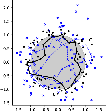
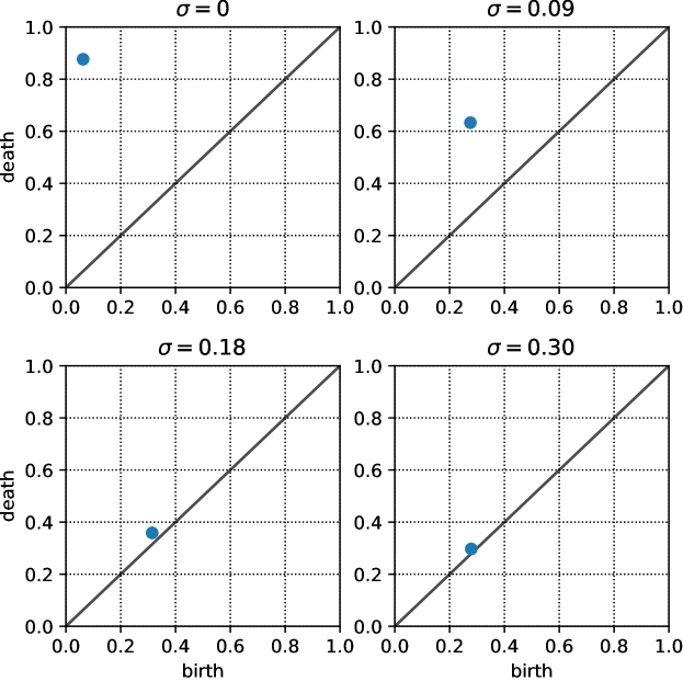
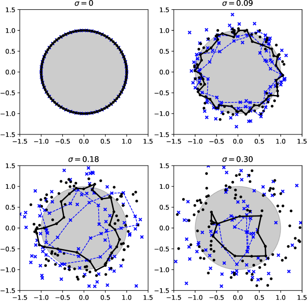
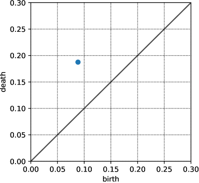
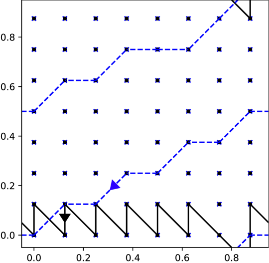
A computational result is presented in Figure 4, which portrays the sampled map at and its unique generator of the persistence diagram. The generator is the corresponding cycle in at the birth radius and is indeed approximating the unit circle, and we can see that its image is turning around the origin twice. Results for other noises are shown in Figure 6.
Figure 6 presents the persistence diagrams under changing from to . As expected, the lifetime of the unique generator decreases as the noise increases.
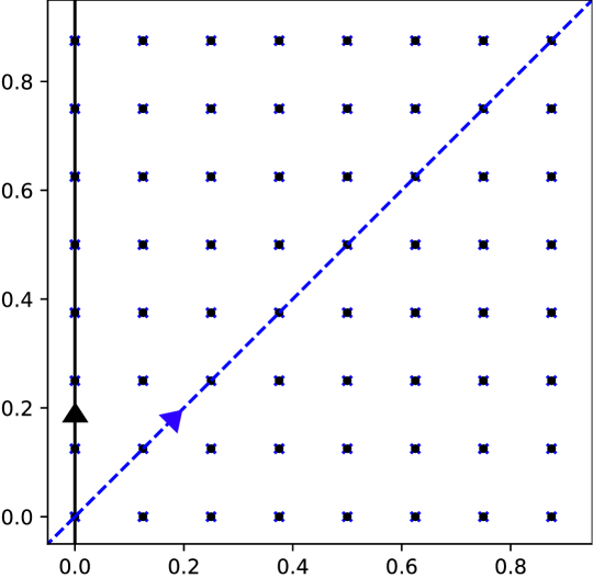
7.2 Inverse mapping on a circle
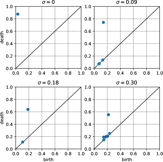
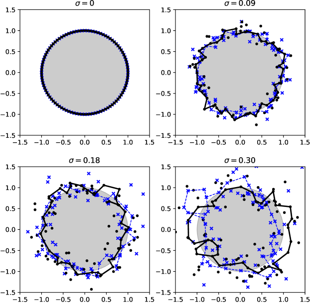
To emphasize the difference from the existing method using eigenspace functors, let us consider the inverse map on the unit circle defined by . The sampled points and the range of the parameter of Gaussian noises are the same as before. The computational results are presented in Figures 8 and 8.
The analysis using eigenspace functors can detect such a generator using the eigenspace functor with eigenvalue . In other words, prior knowledge about the eigenvalue is essential. On the other hand, our method can use the same construction both for the inverse mapping and twice mapping.
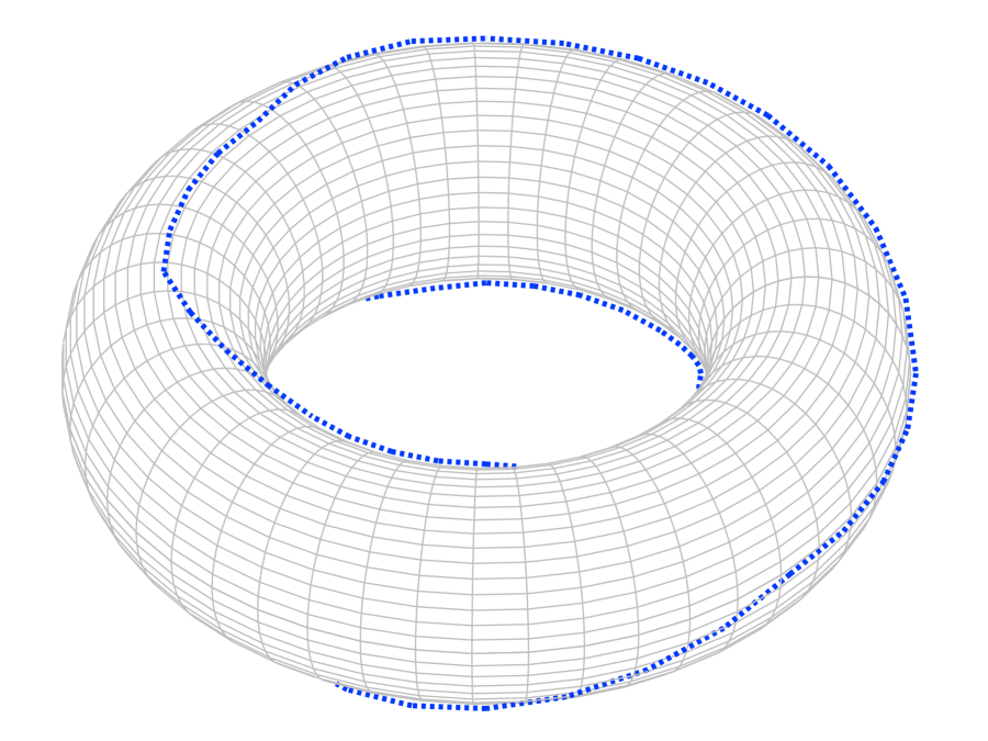
7.3 Mapping on a torus
Moreover, our method can be applied to maps on the torus . We adopt the metric on induced by the Euclidean metric on .
Let us consider the self-map on defined as
| (95) |
We put 64 sampling points and generate a sampled map of on . Such a sampled map of is a challenging example for the analysis using eigenspace without any prior knowledge because the eigenvalues of are and .
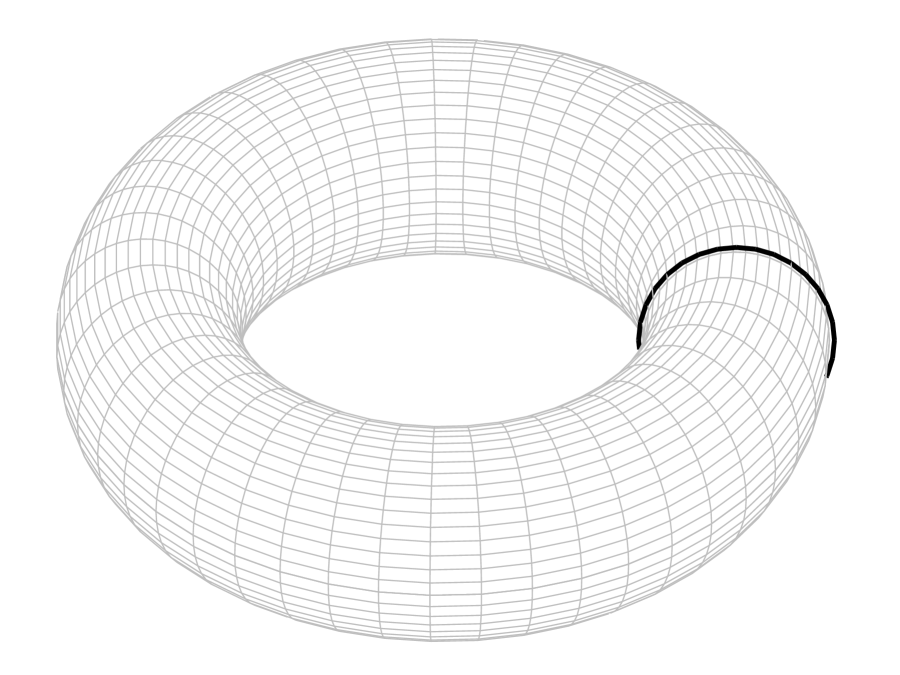
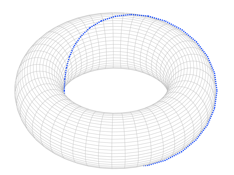
The computational results are presented in Figures 9, 12, 12, 12, 15, 15 and 15. We remark that the unique point in Figure 9 has multiplicity . Let and be a standard homology basis on the torus. The generators corresponding to the unique birth-death point are given by and (= with the coefficient ) in our numerical experiment, where and are cycles in at the birth radius illustrated in Figures 12, 12 and 12 and Figures 15, 15 and 15, respectively. These cycles correspond to the mappings
| (96) |
respectively. The mappings (96) are nothing but the map , concluding the success in reconstructing .
8 Concluding remarks
In this paper, we defined the persistence diagram of a sampled map and proved that the persistence diagram is uniquely determined and independent of the choice of bases in interval decompositions. However, the reconstruction of the homology induced map depended on the choice of the bases of interval decomposition. Our aim is reconstructions of underlying maps, so we must solve the problem on which bases are the best for reconstruction. This problem will be our future work and would be related to the problem on which cycle is optimal for representing the generator of persistent homology [Obayashi 2018].
Acknowledgements
I would like to thank Yasuaki Hiraoka for introducing me to this study, and for many fruitful discussions and stimulating questions. I would like to thank Emerson G. Escolar for important questions about the well-definedness of the persistence analysis. I would like to thank Zin Arai for his constructive suggestions and comments on the paper. I would like to acknowledge the support by Japan Society for the Promotion of Science KAKENHI Grant Number 16J03138, and Japan Science and Technology Agency CREST Mathematics 15656429.
References
- [Asashiba et al. 2019] Asashiba, H., Escolar, E.G., Hiraoka, Y., Takeuchi, H.: Matrix method for persistence modules on commutative ladders of finite type. Jpn. J. Ind. Appl. Math. – (2019)
- [Assem et al. 2006] Assem, I., Simson, D., Skowroński, A.: Elements of the Representation Theory of Associative Algebras 1: Techniques of Representation Theory. Cambridge University Press, Cambridge (2006)
- [Bauer and Lesnick 2014] Bauer, U., Lesnick, M.: Induced Matchings of Barcodes and the Algebraic Stability of Persistence. In Proceedings of the Thirtieth Annual Symposium on Computational Geometry (SoCG ’14), ACM, New York, NY, USA, – (2014)
- [Borsuk 1948] Borsuk, K.: On the imbedding of systems of compacta in simplicial complexes. Fund. Math. 35, – (1948)
- [Carlsson and de Silva 2010] Carlsson, G., de Silva, V.: Zigzag Persistence. Found. Comput. Math. 10, – (2010)
- [Carlsson and Zomorodian 2009] Carlsson, G., Zomorodian, A.: The Theory of Multidimensional Persistence. Discrete Comput. Geom. 42, – (2009)
- [Chazal et al. 2009] Chazal, F., Cohen-Steiner, D., Glisse, M., Guibas, L.J., Oudot, S.Y.: Proximity of Persistence Modules and their Diagrams. In Proceedings of the Twenty-fifth Annual Symposium on Computational Geometry (SoCG ’09), ACM, New York, NY, USA, – (2009)
- [Cohen-Steiner et al. 2007] Cohen-Steiner, D., Edelsbrunner, H., Harer, J.: Stability of Persistence Diagrams. Discrete Comput. Geom. 37, – (2007)
- [Crawley-Boevey 2015] Crawley-Boevey, W.: Decomposition of pointwise finite-dimensional persistence modules. J. Algebra Appl. 14, (2015)
- [Dey et al. 2014] Dey, T.K., Fan, F., Wang, Y.: Computing Topological Persistence for Simplicial Maps. In Proceedings of the Thirtieth Annual Symposium on Computational Geometry (SoCG ’14), ACM, New York, NY, USA, – (2014)
- [Edelsbrunner and Harer 2010] Edelsbrunner, H., Harer, J.: Computational Topology: An Introduction. Amer. Math. Soc., Providence, Rhode Island (2010)
- [Edelsbrunner et al. 2015] Edelsbrunner, H., Jabłoński, G., Mrozek, M.: The Persistent Homology of a Self-Map. Found. Comput. Math. 15, – (2015)
- [Gabriel 1972] Gabriel, P.: Unzerlegbare Darstellungen I. Manuscripta Math. 6, – (1972)
- [Harker et al. 2016] Harker, S., Kokubu, H., Mischaikow, K., Pilarczyk, P.: Inducing a map on homology from a correspondence. Proc. Amer. Math. Soc. 144, – (2016)
- [Lesnick 2015] Lesnick, M.: The Theory of the Interleaving Distance on Multidimensional Persistence Modules. Found. Comput. Math., 15, – (2015)
- [Obayashi 2018] Obayashi, I.: Volume-Optimal Cycle: Tightest Representative Cycle of a Generator in Persistent Homology. SIAM J. Appl. Algebra Geometry, 2(4), – (2018)