Study of Joint Automatic Gain Control and MMSE Receiver Design Techniques for Quantized Multiuser Multiple-Antenna Systems

Abstract

This paper presents the development of a joint optimization of an automatic gain control (AGC) algorithm and a linear minimum mean square error (MMSE) receiver for multi-user multiple input multiple output (MU-MIMO) systems with coarsely quantized signals. The optimization of the AGC is based on the minimization of the mean square error (MSE) and the proposed receive filter takes into account the presence of the AGC and the effects due to quantization. Moreover, we provide a lower bound on the capacity of the MU-MIMO system by deriving an expression for the achievable rate. The performance of the proposed Low-Resolution Aware MMSE (LRA-MMSE) receiver and AGC algorithm is evaluated by simulations, and compared with the conventional MMSE receive filter and Zero-Forcing (ZF) receiver using quantization resolution of 2, 3, 4 and 5 bits.

I INTRODUCTION

In 5G celular systems, high data rates, reliable links, low cost and power consumption are key requirements. Multiple-input multiple-output (MIMO) systems in wireless communications provide significant improvements in wireless link reliability and achievable rates. However, as the number of antennas scales up, the energy consumption and circuit complexity increases accordingly [1, 2, 3, 4, 5]. For example, the energy consumption of an analog to digital converter (ADC) grows exponentially as a function of the quantization resolution. To reduce circuit complexity and save energy, novel transmission approaches employ low resolution ADCs, which generate significant nonlinear distortion and, thus, require new signal processing techniques to provide reliable data transmission. Several studies present detection methods that deal with signals quantized with few bits of resolution [1, 6, 2, 4].

Automatic gain control (AGC) is the process of adjusting the analog signal level to the dynamic range of the analog to digital converter (ADC) in order to minimize the signal distortion due to the quantization [7]. The use of an AGC is important in applications where the received power varies over time, as is the case in mobile scenarios. Proper AGC design becomes especially important for low resolution ADCs. Although there are many articles on quantization in MIMO systems in the literature, few address the design of AGCs. In [1], the authors presented a modified MMSE receiver that takes into account the quantization effects in a MIMO system but they do not take into account the presence of an AGC. The effects of an AGC on a quantized MIMO system with a standard Zero-Forcing filter at the receiver were examined in [6]. However, the authors have not optimized the AGC algorithm nor used a detector that considers the quantization effects.

This work presents a framework for jointly designing the AGC and a linear receive filter according to the MMSE criterion for a large-scale MU-MIMO system operating with coarsely quantized signals. The procedure consists of computing the modified MMSE receiver presented in [1] and, after that, computing the derivative of the cost function that takes into account the presence of the AGC in order to obtain the optimal AGC coefficients. Then, a Low-Resolution Aware MMSE (LRA-MMSE) receiver that considers both quantization effects and the AGC is derived. A lower bound on the capacity of this system is investigated and an expression to compute the achievable rates is developed.

Notation: Vectors and matrices are denoted by lower and upper case italic bold letters. The operators $(\cdot)^{T}$, $(\cdot)^{H}$ and $\mathop{\rm tr}(\cdot)$ stand for transpose, Hermitian transpose and trace of a matrix, respectively. $\mathbf{1}$ denotes a column vector of ones and $\mathbf{I}$ denotes an identity matrix. The operator $E[\cdot]$ stands for expectation with respect to the random variables and the operator $\odot$ corresponds to the Hadamard product. Finally, $\mathop{\rm diag}(\mathbf{A})$ denotes a diagonal matrix containing only the diagonal elements of $\mathbf{A}$ and $\mathop{\rm nondiag}(\mathbf{A})=\mathbf{A}-\mathop{\rm diag}(\mathbf{A})$.

II System Description

A large-scale uplink MU-MIMO system [12, 14] consisting of a base station (BS) with $N_{R}$ receive antennas, and $K$ users equipped with $N_{T}$ transmit antennas each is considered. At each time instant $i$, each user transmits $N_{T}$ symbols which are organized into a $N_{T}\times 1$ vector $\mathbf{x}_{k}[i]=[x_{1}[i],x_{2}[i],...,x_{N_{T}}[i]]^{T}$. Each entry of the vector $\mathbf{x}_{k}[i]$ is a symbol taken from the modulation alphabet $\mathbb{A}$. The symbol vector is then transmitted through flat fading channels and corrupted by additive white Gaussian noise (AWGN). The received signal collected by the receive antennas at the BS is given by the following equation:

$$\mathbf{y}[i]=\sum_{k=1}^{K}\mathbf{H}_{k}\mathbf{x}_{k}[i]+\mathbf{n}[i]=\mathbf{H}\mathbf{x}[i]+\mathbf{n}[i],$$ (1)

where $\mathbf{y}[i]\in\mathbb{C}^{N_{R}\times 1}$, and $\mathbf{H}_{k}\in\mathbb{C}^{N_{R}\times N_{T}}$ is a matrix that contains the complex channel gains from the $N_{T}$ transmit antennas of user $k$ to the $N_{R}$ receive antennas of the BS. The $N_{R}\times 1$ vector $\mathbf{n}[i]$ is a zero-mean complex circular symmetric Gaussian noise vector with covariance matrix $E[\mathbf{n}[i]\mathbf{n}^{H}[i]]=\sigma_{n}^{2}\mathbf{I}$. $\mathbf{H}$ is a $N_{R}\times KN_{T}$ matrix that contains the coefficients of the flat fading channels between the transmit antennas of the $K$ users and the receive antennas of the BS. The symbol vector $\mathbf{x}[i]=[\mathbf{x}_{1}[i],...,\mathbf{x}_{k}[i],...,\mathbf{x}_{K}[i]]^{T}$ contains all symbols that are transmitted by the users at time instant $i$. The channel state information (CSI) is assumed to be unknown to the users at the transmit side. Therefore, we assume the same symbol energy per user and transmit antenna, i.e. $E[\mathbf{x}\mathbf{x}^{H}]=\sigma_{x}^{2}\mathbf{I}$.

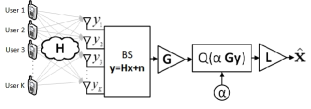
Figure 1: An uplink quantized MU-MIMO system

As depicted in Fig.1, before to be quantized, $\mathbf{y}$ is jointly pre-multiplied by the clipping level factor $\alpha$ and the AGC matrix $\mathbf{G}$ to minimizes the granular and the overload distortions. After that, the product $\alpha\mathbf{G}\mathbf{y}$ is quantized and the estimation of the transmitted symbol vector $\mathbf{x}$ is performed by the LRA-MMSE receiver, represented by $\mathbf{L}$. The estimated symbol vector is represented by $\hat{\mathbf{x}}$. The real, $y_{i,R}$, and imaginary, $y_{i,I}$, parts of the complex received signal at each antenna are quantized separately by uniform $b$-bit resolution ADCs. Therefore, the resulting quantized signals read as

$$r_{i,l}=Q(y_{i,l})=y_{i,l}+q_{i,l},\hskip 4.0ptl\in\{R,I\},\hskip 4.0pt1\leq i\leq N_{R},$$ (2)

where $Q(\cdot)$ denotes the quantization operation and $q_{i,l}$ is the resulting quantization error.

The distortion factor indicates the relative amount of quantization noise generated by the quantizer, and is given by $\rho_{q}^{(i,l)}=\sigma_{q_{i,l}}^{2}/\sigma_{y_{i,l}}^{2}$, where $\sigma_{q_{i,l}}^{2}$ is the variance of the quantizer error and, $\sigma_{y_{i,l}}^{2}$ is the variance of the input $y_{i,l}$. This factor depends on the number of quantization bits $b$, the quantizer type, and the probability density function of $y_{i,l}$ [1]. In this work the scalar uniform quantizer processes the real and imaginary parts of the input signal $y_{i,l}$ in a range $\pm\frac{\sqrt{b}}{2}$. With a high number of antennas the input signals of the quantizer are approximately Gaussian distributed and they undergo nearly the same distortion factor $\rho_{q}$. It was shown in [8] for the uniform quantizer case, that optimal quantization step $\Delta$ for a Gaussian source decreases as $\sqrt{b}2^{-b}$ and that $\rho_{q}$ is asymptotically well approximated by $\frac{\Delta^{2}}{12}$.

III Proposed Joint AGC and Linear MMSE Receiver Design

The procedure for joint optimization of the AGC algorithm and the LRA-MMSE receiver carries out alternating computations between the AGC and the LRA-MMSE receiver. The first step consists of computing an LRA-MMSE receive filter that considers the quantization effects. Other approaches to computing linear MMSE or related filters [18, 19, 20, 21] can also be considered. After that, we compute the derivative of the cost function to obtain the optimal AGC coefficients. Then, an updated LRA-MMSE receiver is computed.

III-A Linear LRA-MMSE Receive Filter Design

In this first step we do not consider the presence of the AGC in the system. Thus, the received signal after the quantizer is expressed, with the Bussgang decomposition [9], as a linear model $\mathbf{r}=\mathbf{y}+\mathbf{q}$. To develop the linear receive filter $\mathbf{W}$ that minimizes the MSE we use the Wiener-Hopf equations:

$$\mathbf{W}=\mathbf{R}_{xr}\mathbf{R}_{rr}^{-1},$$ (3)

where the auto-correlation matrix $\mathbf{R}_{rr}$ is given by

$$\mathbf{R}_{rr}=E[\mathbf{r}\mathbf{r}^{H}]=\mathbf{R}_{yy}+\mathbf{R}_{yq}+\mathbf{R}_{yq}^{H}+\mathbf{R}_{qq},$$ (4)

and the cross-correlation matrix $\mathbf{R}_{xr}$ can be expressed as

$$\mathbf{R}_{xr}=E[\mathbf{x}\mathbf{r}^{H}]=\mathbf{R}_{xy}+\mathbf{R}_{xq}$$ (5)

We get the auto-correlation matrix $\mathbf{R}_{yy}$ and the cross-correlation matrix $\mathbf{R}_{xy}$ directly from the MIMO model as

$$\mathbf{R}_{yy}=E[\mathbf{y}\mathbf{y}^{H}]=\mathbf{H}\mathbf{R}_{xx}\mathbf{H}^{H}+\mathbf{R}_{nn}$$ (6)

and,

$$\mathbf{R}_{xy}=E[\mathbf{x}\mathbf{y}^{H}]=\mathbf{R}_{xx}\mathbf{H}^{H}$$ (7)

To compute (4) and (5) we need to obtain the covariance matrices $\mathbf{R}_{yq}$, $\mathbf{R}_{qq}$ and $\mathbf{R}_{xq}$ as a function of the channel parameters and the distortion factor $\rho_{q}$. The procedure of how to obtain these matrices was developed in [1] and we will use some of these results in this work. The cross-correlation between the received signal vector and the quantization error is approximated by

$$\mathbf{R}_{yq} \approx -\rho_{q}\mathbf{R}_{yy}$$ (8)

The covariance matrix of the quantization error is deduced from

$$\mathbf{R}_{qq} \approx \rho_{q}\mathop{\rm diag}(\mathbf{R}_{yy})+\rho_{q}^{2}\mathop{\rm nondiag}(\mathbf{R}_{yy})$$ (9)

$$= \rho_{q}\mathbf{R}_{yy}-(1-\rho_{q})\rho_{q}\mathop{\rm nondiag}(\mathbf{R}_{yy}),$$

and the cross-correlation matrix between the desired signal vector and the quantization error can be obtained by

$$\mathbf{R}_{xq}=-\rho_{q}\mathbf{R}_{xy}$$ (10)

Substituting (10) in (5) we get

$$\mathbf{R}_{xr}=(1-\rho_{q})\mathbf{R}_{xy}$$ (11)

and substituting (6), (8) and (9) in (4) we get

$$\mathbf{R}_{rr}\approx(1-\rho_{q})(\mathbf{R}_{yy}-\rho_{q}\mathop{\rm nondiag}(\mathbf{R}_{yy}))$$ (12)

Finally, by substituting (11) and (12) in (3) we get the expression of the LRA-MMSE receive filter for a quantized MU-MIMO system. As shown in [1], we can write this solution as

$$\mathbf{W}=\mathbf{R}_{xy}(\mathbf{R}_{yy}-\rho_{q}\mathop{\rm nondiag}(\mathbf{R}_{yy}))^{-1}$$ (13)

With the presence of the AGC the expression of the received vector changes and can be computed by $\mathbf{z}=\mathbf{G}\mathbf{y}+\mathbf{q}$. With the same procedure as before, the MMSE filter with AGC can be computed through the Wiener-Hopf equations as $\mathbf{L}=\mathbf{R}_{xz}\mathbf{R}_{zz}^{-1}$. The auto-correlation matrix $\mathbf{R}_{zz}$ and the cross-correlation matrix $\mathbf{R}_{xz}$ can be computed similarly by

$$\mathbf{R}_{zz} = E[\mathbf{z}\mathbf{z}^{H}]=\mathbf{G}\mathbf{R}_{yy}\mathbf{G}+\mathbf{G}\mathbf{R}_{yq}+\mathbf{R}_{yq}^{H}\mathbf{G}+\mathbf{R}_{qq}$$

$$\mathbf{R}_{xz} = E[\mathbf{x}\mathbf{z}^{H}]=\mathbf{R}_{xy}\mathbf{G}+\mathbf{R}_{xq}$$

We note that nonlinear receiver structures can also be considered following the approaches reported in [22, 23, 24, 25, 26].

III-B AGC Design

In [6], the authors proposed a standard AGC algorithm by using a diagonal matrix $\mathbf{G}$ with real coefficients. This matrix is used to compensate the gain differences of the propagation channel and involves a search over a transmitted symbol alphabet. This approach is very computationally demanding in an environment with a high number of antennas. Writing $\mathbf{G}$ as $\mathop{\rm diag}(\mathbf{g})$, where $\mathbf{g}$ is a column vector with the diagonal elements of $\mathbf{G}$, the proposed AGC algorithm is based on the minimization of the cost function:

$$\varepsilon = E[||\mathbf{x}-\hat{\mathbf{x}}||^{2}]$$ (14)

$$= E[||\mathbf{x}-\mathbf{W}(\alpha\mathop{\rm diag}(\mathbf{g})\mathbf{y}+\mathbf{q})||^{2}]$$

and since $\mathbf{G}$ is a diagonal matrix with real coefficients we have $\mathop{\rm diag}(\mathbf{g})^{H}=\mathop{\rm diag}(\mathbf{g})$. Then,

$$\varepsilon= \mathop{\rm tr}(\mathbf{R}_{xx}-\alpha\mathbf{R}_{xy}\mathop{\rm diag}(\mathbf{g})\mathbf{W}^{H}-\mathbf{R}_{xq}\mathbf{W}^{H}$$

$$-\alpha\mathbf{W}\mathop{\rm diag}(\mathbf{g})\mathbf{R}_{xy}^{H}+\alpha^{2}\mathbf{W}\mathop{\rm diag}(\mathbf{g})\mathbf{R}_{yy}\mathop{\rm diag}(\mathbf{g})\mathbf{W}^{H}$$

$$+\alpha\mathbf{W}\mathop{\rm diag}(\mathbf{g})\mathbf{R}_{yq}\mathbf{W}^{H}-\mathbf{W}\mathbf{R}_{xq}^{H}$$

$$+\alpha\mathbf{W}\mathbf{R}_{yq}^{H}\mathop{\rm diag}(\mathbf{g})\mathbf{W}^{H}+\mathbf{W}\mathbf{R}_{qq}\mathbf{W}^{H})$$

To obtain the optimum $\mathbf{G}$ matrix we compute the derivative of the MSE cost function with respect to $\mathop{\rm diag}(\mathbf{g})$, equate the derivative terms to zero and solve for $\mathbf{g}$:

$$\frac{\partial\varepsilon}{\partial\mathbf{g}}= -\alpha\underbrace{\frac{\partial}{\partial\mathbf{g}}\mathop{\rm tr}(\mathbf{R}_{xy}\mathop{\rm diag}(\mathbf{g})\mathbf{W}^{H}}_{I})-\alpha\underbrace{\frac{\partial}{\partial\mathbf{g}}\mathop{\rm tr}(\mathbf{W}\mathop{\rm diag}(\mathbf{g})\mathbf{R}_{xy}^{H}}_{II})$$

$$+\alpha^{2}\underbrace{\frac{\partial}{\partial\mathbf{g}}\mathop{\rm tr}(\mathbf{W}\mathop{\rm diag}(\mathbf{g})\mathbf{R}_{yy}\mathop{\rm diag}(\mathbf{g})\mathbf{W}^{H}}_{III})$$

$$+\alpha\underbrace{\frac{\partial}{\partial\mathbf{g}}\mathop{\rm tr}(\mathbf{W}\mathop{\rm diag}(\mathbf{g})\mathbf{R}_{yq}\mathbf{W}^{H}}_{IV})$$

$$+\alpha\underbrace{\frac{\partial}{\partial\mathbf{g}}\mathop{\rm tr}(\mathbf{W}\mathbf{R}_{yq}^{H}\mathop{\rm diag}(\mathbf{g})\mathbf{W}^{H})}_{V}$$ (15)

We have to take the derivative of each term of Eq. (15). Consider the conversion between matrix notation and index notation and the tricky case of a $\mathop{\rm diag}(\cdot)$ operator

$$[\mathbf{A}\mathbf{B}]_{ik}=\sum_{j}A_{ij}B_{jk}$$ (16)

$$f=\mathop{\rm tr}[\mathbf{A}\mathop{\rm diag}(\mathbf{g})\mathbf{B}]=\sum_{i}\sum_{j}A_{ij}g_{j}B_{ji}$$ (17)

Taking the derivative with respect to the coefficients $g_{j}$ of the diagonal operator we have

$$\frac{\partial f}{\partial g_{j}}=\sum_{i}A_{ij}B_{ji}=[(\mathbf{A}^{T}\odot\mathbf{B})\mathbf{1}]_{j}$$ (18)

Therefore, we can write

$$\frac{\partial\mathop{\rm tr}[\mathbf{A}\mathop{\rm diag}(\mathbf{g})\mathbf{B}]}{\partial\mathbf{g}}=(\mathbf{A}^{T}\odot\mathbf{B})\mathbf{1}$$ (19)

With these considerations we can take the derivative of terms $I$ , $II$, $III$, $IV$ and $V$ from Eq. (15). The derivatives of the terms $I$ and $II$ can be computed by

$$I=\frac{\partial\mathop{\rm tr}[\mathbf{R}_{xy}\mathop{\rm diag}(\mathbf{g})\mathbf{W}^{H}]}{\partial\mathbf{g}}=[(\mathbf{R}_{xy}^{T}\odot\mathbf{W}^{H})\mathbf{1}]$$ (20)

$$II=\frac{\partial\mathop{\rm tr}[\mathbf{W}\mathop{\rm diag}(\mathbf{g})\mathbf{R}_{xy}^{H}]}{\partial\mathbf{g}}=[(\mathbf{R}_{xy}^{H}\odot\mathbf{W}^{T})\mathbf{1}]$$ (21)

To compute the derivative of term $III$ we apply the chain rule

$$III=\underbrace{\frac{\partial\mathop{\rm tr}[\mathbf{W}\mathop{\rm diag}(\mathbf{g})\mathbf{A}]}{\partial\mathbf{g}}}_{III.1}+\underbrace{\frac{\partial tr[\mathbf{B}\mathop{\rm diag}(\mathbf{g})\mathbf{W}^{H}]}{\partial\mathbf{g}}}_{III.2}$$ (22)

where $\mathbf{A}=\mathbf{R}_{yy}\mathop{\rm diag}(\mathbf{g})\mathbf{W}^{H}$ and $\mathbf{B}=\mathbf{W}\mathop{\rm diag}(\mathbf{g})\mathbf{R}_{yy}$. The term $III.1$ can be computed by

$$III.1=[(\mathbf{W}^{T}\odot(\mathbf{R}_{yy}\mathop{\rm diag}(\mathbf{g})\mathbf{W}^{H}))\mathbf{1}]$$ (23)

and the term $III.2$ as

$$III.2=[((\mathbf{R}_{yy}^{T}\mathop{\rm diag}(\mathbf{g})\mathbf{W}^{T})\odot\mathbf{W}^{H})\mathbf{1}]$$ (24)

Substituting (23) and (24) in (25) we have

$$III= [(\mathbf{W}^{T}\odot(\mathbf{R}_{yy}\mathop{\rm diag}(\mathbf{g})\mathbf{W}^{H}))\mathbf{1}]$$ (25)

$$+ [((\mathbf{R}_{yy}^{T}\mathop{\rm diag}(\mathbf{g})\mathbf{W}^{T})\odot\mathbf{W}^{H})\mathbf{1}]$$

The derivative of the term $IV$ is given by

$$IV=\frac{\partial tr[\mathbf{W}\mathop{\rm diag}(\mathbf{g})\mathbf{C}]}{\partial\mathbf{g}}=[(\mathbf{W}^{T}\odot(\mathbf{R}_{yq}\mathbf{W}^{H}))\mathbf{1}]\textbf{}$$ (26)

where $\mathbf{C}=\mathbf{R}_{yq}\mathbf{W}^{H}$. Finally, the derivative of the term $V$ can be computed by

$$V=\frac{\partial\mathop{\rm tr}[\mathbf{D}\mathop{\rm diag}(\mathbf{g})\mathbf{W}^{H}]}{\partial\mathbf{g}}=[((\mathbf{R}_{yq}^{*}\mathbf{W}^{T})\odot\mathbf{W}^{H})\mathbf{1}]$$ (27)

where $\mathbf{D}=\mathbf{W}\mathbf{R}_{yq}^{H}$. Substituting (20), (21), (25), (26) and (27) in (15) and equating the derivatives to zero we have

$$[\mathbf{W}^{T}\odot(\mathbf{R}_{yy}\mathop{\rm diag}(\mathbf{g})\mathbf{W}^{H})+(\mathbf{R}_{yy}^{T}\mathop{\rm diag}(\mathbf{g})\mathbf{W}^{T})\odot\mathbf{W}^{H}]\mathbf{1}=$$

$$\frac{1}{\alpha}([(\mathbf{R}_{xy}^{T}\odot\mathbf{W}^{H})\mathbf{1}]+[(\mathbf{R}_{xy}^{H}\odot\mathbf{W}^{T})\mathbf{1}]+$$

$$-[(\mathbf{W}^{T}\odot(\mathbf{R}_{yq}\mathbf{W}^{H}))\mathbf{1}]-[((\mathbf{R}_{yq}^{*}\mathbf{W}^{T})\odot\mathbf{W}^{H})\mathbf{1}])$$ (28)

To achieve the desired $\mathbf{g}$ we have to do some manipulations with the first term of (28). To do this we will write the first and second terms of $\mathbf{g}$ with the index notation and after that we will return to the matrix notation. We can write the first term as

$$[(\mathbf{W}^{T}\odot(\mathbf{R}_{yy}\mathop{\rm diag}(\mathbf{g})\mathbf{W}^{H})\mathbf{1}]=\sum_{j=1}^{KN_{T}}\sum_{l=1}^{N_{R}}W_{ji}R_{yy,il}g_{l}W_{lj}^{H}$$ (29)

and the second term as

$$[(\mathbf{W}^{H}\odot(\mathbf{R}_{yy}^{T}\mathop{\rm diag}(\mathbf{g})\mathbf{W}^{T})\mathbf{1}]=\sum_{j=1}^{KN_{T}}\sum_{l=1}^{N_{R}}W_{ij}^{H}R_{yy,li}g_{l}W_{jl}$$ (30)

With some manipulations we can isolate the vector $\mathbf{g}$

$$[\mathbf{W}^{T}\odot(\mathbf{R}_{yy}\mathop{\rm diag}(\mathbf{g})\mathbf{W}^{H})+\mathbf{W}^{H}\odot(\mathbf{R}_{yy}^{T}\mathop{\rm diag}(\mathbf{g})\mathbf{W}^{T})]\mathbf{1}$$

$$=\sum_{j=1}^{KN_{T}}\sum_{l=1}^{N_{R}}W_{ji}R_{yy,il}g_{l}W_{lj}^{H}+\sum_{j=1}^{KN_{T}}\sum_{l=1}^{N_{R}}W_{ij}^{H}R_{yy,li}g_{l}W_{jl}$$

$$=\sum_{l=1}^{N_{R}}([(\mathbf{W}^{T}\mathbf{W}^{*})\odot\mathbf{R}_{yy}+(\mathbf{W}^{H}\mathbf{W})\odot\mathbf{R}_{yy}^{T}]_{il})g_{l}$$

$$=[(\mathbf{W}^{T}\mathbf{W}^{*})\odot\mathbf{R}_{yy}+(\mathbf{W}^{H}\mathbf{W})\odot\mathbf{R}_{yy}^{T}]\mathbf{g}$$ (31)

Substituting (31) in (28) and solving with respect to $\mathbf{g}$ we have

$$\mathbf{g}= [(\mathbf{W}^{T}\mathbf{W}^{*})\odot\mathbf{R}_{yy}+(\mathbf{W}^{H}\mathbf{W})\odot\mathbf{R}_{yy}^{T}]^{-1}$$

$$\cdot\frac{2}{\alpha}(Re([(\mathbf{R}_{xy}^{T}\odot\mathbf{W}^{H})\mathbf{1}])-Re([(\mathbf{W}^{T}\odot\mathbf{R}_{yq}\mathbf{W}^{H})\mathbf{1}]))$$ (32)

IV Clip-level adjustment

In the following we outline the computation of the clipping factor $\alpha$ based on the signal power. This factor conforms the received signal power between the quantizer range to minimize the overload distortion. The received signal power can be computed by

$$P = \mathop{\rm tr}(E[(\mathbf{y}+\mathbf{q})(\mathbf{y}+\mathbf{q})^{H}])$$ (33)

$$= \mathop{\rm tr}(\mathbf{R}_{yy}+\mathbf{R}_{yq}+\mathbf{R}_{yq}^{H}+\mathbf{R}_{qq})$$

and received symbol energy by

$$E_{rx}=\sqrt{\frac{\mathop{\rm tr}(\mathbf{R}_{yy}+\mathbf{R}_{yq}+\mathbf{R}_{yq}^{H}+\mathbf{R}_{qq})}{N_{R}}}$$ (34)

Thus, the clipping factor $\alpha$ can be obtained from

$$\alpha=\beta\cdot\sqrt{\frac{tr(\mathbf{R}_{yy}+\mathbf{R}_{yq}+\mathbf{R}_{yq}^{H}+\mathbf{R}_{qq})}{N_{R}}},$$ (35)

where $\beta$ is a calibration factor. In our simulations the value of $\beta$ was set to $\sqrt{b}$ which corresponds to the quantizer output range, to ensure an optimized performance.

V Capacity lower bound

In [1] a lower bound on the mutual information between the input sequence $\mathbf{x}$ and the quantized output sequence $\mathbf{r}$ of a quantized MIMO system was developed, based on the MSE approach. We will use a similar procedure to consider a capacity lower bound of our quantized MU-MIMO system with the optimal AGC and to derive an expression for computing the achievable rates for the proposed AGC and LRA-MMSE receiver. We remark that similar analyses can be considered for the downlink with the use of precoding techniques [15, 16, 17]. As described in [11] the mutual information of this channel can be expressed as

$$I(\mathbf{x},\mathbf{r})=h(\mathbf{x})-h(\mathbf{x}|\mathbf{r})$$ (36)

Given $\mathbf{R}_{xx}$ under a power contraint $tr(\mathbf{R}_{xx})\leq P_{\mathop{\rm Tr}}$, we choose $\mathbf{x}$ to be Gaussian, which is not necessarily the capacity achieving distribution for our quantized system. Then, we can obtain a lower bound for $I(\mathbf{x},\mathbf{r})$ (in bit/transmission) as

$$I(\mathbf{x},\mathbf{r}) = \log_{2}\det(\mathbf{R}_{xx})-h(\mathbf{x}|\mathbf{r})$$ (37)

$$= \log_{2}\det(\mathbf{R}_{xx})-h(\mathbf{x}-\hat{\mathbf{x}}|\mathbf{r})$$

$$\geq \log_{2}\det(\mathbf{R}_{xx})-h(\underbrace{\mathbf{x}-\hat{\mathbf{x}}}_{\epsilon})$$

$$\geq \log_{2}\frac{\det(\mathbf{R}_{xx})}{\det(\mathbf{R}_{\epsilon\epsilon})}$$ (38)

The second term in (37) is upper bounded by the entropy of a Gaussian random variable whose covariance is equal to the error covariance matrix $\mathbf{R}_{\epsilon\epsilon}$ of the LRA-MMSE estimate of $\mathbf{x}$. Thus, we have to compute the expressions of $\mathbf{R}_{xx}$ and $\mathbf{R}_{\epsilon\epsilon}$ for our system. Considering unknown CSI at the transmitter, the autocorrelation matrix $\mathbf{R}_{xx}$ is given by

$$\mathbf{R}_{xx}=\sigma_{x}^{2}\mathbf{I}_{KN_{T}},$$ (39)

and the error covariance matrix can be computed by

$$\mathbf{\mathbf{R}_{\epsilon\epsilon}}= E[(\mathbf{x}-\hat{\mathbf{x}})(\mathbf{x}-\hat{\mathbf{x}})^{H}]$$

$$= \mathbf{R}_{xx}-\mathbf{R}_{xy}\mathbf{G}\mathbf{W}^{H}-\mathbf{R}_{xq}\mathbf{W}^{H}-\mathbf{W}\mathbf{G}\mathbf{R}_{xy}^{H}+$$

$$+\mathbf{W}\mathbf{G}\mathbf{R}_{yy}\mathbf{G}\mathbf{W}^{H}+\mathbf{W}\mathbf{G}\mathbf{R}_{yq}\mathbf{W}^{H}-\mathbf{W}\mathbf{R}_{xq}^{H}+$$

$$+\mathbf{W}\mathbf{R}_{yq}^{H}\mathbf{G}\mathbf{W}^{H}+\mathbf{W}\mathbf{R}_{qq}\mathbf{W}^{H}$$ (40)

Substituting (39) and (40) in (38) we obtain an expression to compute the achievable rates for the MU-MIMO system with coarsely quantized signals.

VI Results

To evaluate the results obtained in previous sections we consider a MU-MIMO system with $K=16$ users who are each equipped with $N_{T}=2$ transmit antennas and one BS with $N_{R}=64$ receive antennas. At each time instant the users transmit data packets with 100 symbols using BPSK modulation. The channels are obtained with independent and identically distributed complex Gaussian random variables with zero mean and unit variance. For each simulation 10000 packets are transmitted, by each transmit antenna, over a flat-fading channel. The received signal is quantized with 2, 3, 4 and 5 bits.

Figure 2: Joint AGC and LRA-MMSE receiver performance comparison

Fig. 2 shows the BER performance of the proposed joint AGC and LRA-MMSE receiver design. As expected, the standard MMSE detector achieved, even in a quantized environment, a better performance than the ZF detector. This occurs because the MMSE filter incorporates the variance of the receive antenna noise which improves the accuracy of the MMSE detector at low SNR values. Moreover, we can see that among all receivers the LRA-MMSE with the proposed AGC obtained the best performance. The design of this receiver aggregates the gains by incorporating the AGC and the effects due to the coarse quantization. The curves also show that, with the presented approximations, the joint AGC and LRA-MMSE receiver design achieves a performance very close to the performance of the Full Resolution standard MMSE receiver (FR standard MMSE).

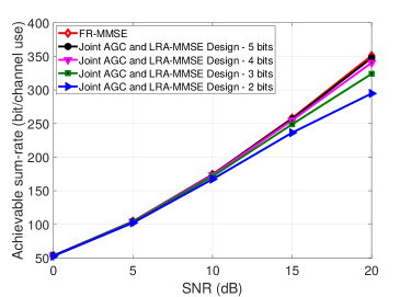
Figure 3: Achievable sum-rate of the quantized MU-MIMO system with 32 users with 2 transmit antennas each and one BS with 64 receive antennas.

In Fig. 3 we illustrate the achievable sum rates of the MU-MIMO system with the joint AGC and LRA-MMSE receiver design for different numbers of quantization bits. This result shows that, as the number of quantization bits increases, the sum-rate also increases approaching those values obtained by the FR standard MMSE receiver in an unquantized environment.

VII Conclusions

In this work we have discussed the joint design of an AGC and a LRA-MMSE receive filter for coarsely quantized MU-MIMO systems. Simulations results have shown that the joint AGC and the LRA-MMSE receiver obtained a performance close to the full resolution MMSE receiver in a quantized MU-MIMO system with 4 and 5 bits of resolution. Furthermore, we have derived an expression for computing the achievable rates for the system. The results have shown that with 4 and 5 quantization bits we achieve a rate very close to the capacity of an unquantized large-scale MU-MIMO system.

References

- [1] A. Mezghani, M. S. Khoufi, and J. A. Nossek, "A Modified MMSE Receiver for Quantized MIMO Systems," in Proc. ITG/IEEE WSA, Vienna, Austria, February 2007.
- [2] A. Mezghani, M. Rouatbi and J. A. Nossek, "An iterative receiver for quantized MIMO systems," in 2012 16th IEEE Mediterranean Electrotechnical Conference, Yasmine Hammamet, 2012, pp. 1049-1052.
- [3] L. T. N. Landau and R. C. de Lamare, "Branch-and-Bound Precoding for Multiuser MIMO Systems With 1-Bit Quantization," in IEEE Wireless Communications Letters, vol. 6, no. 6, pp. 770-773, Dec. 2017.
- [4] Z. Shao, R. C. de Lamare and L. T. N. Landau, "Iterative Detection and Decoding for Large-Scale Multiple-Antenna Systems With 1-Bit ADCs," in IEEE Wireless Communications Letters, vol. 7, no. 3, pp. 476-479, June 2018.
- [5] L. T. N. Landau, M. Doerpinghaus, R. C. de Lamare and G. P. Fettweis, "Achievable Rate With 1-Bit Quantization and Oversampling Using Continuous Phase Modulation-Based Sequences," in IEEE Transactions on Wireless Communications, vol. 17, no. 10, pp. 7080-7095, Oct. 2018.
- [6] B. M. Murray and I. B. Collings, "AGC and Quantization Effects in a Zero-Forcing MIMO Wireless System," in 2006 IEEE 63rd Vehicular Technology Conference, Melbourne, Vic., 2006, pp. 1802-1806.
- [7] M. Kim, G. Jo and J. Kim, "Optimal detection considering AGC effects in multiple antenna systems," 2008 IEEE International Symposium on Consumer Electronics," Vilamoura, 2008, pp. 1-4.
- [8] D. Hui and D. L. Neuhoff, "Asymptotic analysis of optimal fixed-rate uniform scalar quantization," in IEEE Transactions on Information Theory," vol. 47, no. 3, pp. 957-977, Mar 2001.
- [9] J. J. Bussgang, "Crosscorrelation functions of amplitude-distorted Gaussian signals," Technical Report No. 216, Research Laboratory of Electronics, Massachusetts Institute of Technology, Cambridge, MA, Mar. 1952
- [10] J. Max, "Quantizing for minimum distortion," in IRE Transactions on Information Theory," vol. 6, no. 1, pp. 7-12, March 1960.
- [11] T. M. Cover and J. A. Thomas, Elements of information Theory, John Wiley and Son, New York, 1991.
- [12] R. C. de Lamare, "Massive MIMO systems: Signal processing challenges and future trends," in URSI Radio Science Bulletin, vol. 2013, no. 347, pp. 8-20, Dec. 2013.
- [13] Y. Dong and L. Qiu, "Spectral Efficiency of Massive MIMO Systems With Low-Resolution ADCs and MMSE Receiver," in IEEE Communications Letters, vol. 21, no. 8, pp. 1771-1774, Aug. 2017.
- [14] W. Zhang et al., "Large-Scale Antenna Systems With UL/DL Hardware Mismatch: Achievable Rates Analysis and Calibration," in IEEE Transactions on Communications, vol. 63, no. 4, pp. 1216-1229, April 2015.
- [15] K. Zu, R. C. de Lamare and M. Haardt, "Generalized Design of Low-Complexity Block Diagonalization Type Precoding Algorithms for Multiuser MIMO Systems," in IEEE Transactions on Communications, vol. 61, no. 10, pp. 4232-4242, October 2013.
- [16] W. Zhang et al., "Widely Linear Precoding for Large-Scale MIMO with IQI: Algorithms and Performance Analysis," in IEEE Transactions on Wireless Communications, vol. 16, no. 5, pp. 3298-3312, May 2017.
- [17] K. Zu, R. C. de Lamare and M. Haardt, "Multi-Branch Tomlinson-Harashima Precoding Design for MU-MIMO Systems: Theory and Algorithms," in IEEE Transactions on Communications, vol. 62, no. 3, pp. 939-951, March 2014.
- [18] R. C. de Lamare and R. Sampaio-Neto, "Adaptive Reduced-Rank Processing Based on Joint and Iterative Interpolation, Decimation, and Filtering," in IEEE Transactions on Signal Processing, vol. 57, no. 7, pp. 2503-2514, July 2009.
- [19] R. C. de Lamare and R. Sampaio-Neto, "Reduced-Rank Adaptive Filtering Based on Joint Iterative Optimization of Adaptive Filters," in IEEE Signal Processing Letters, vol. 14, no. 12, pp. 980-983, Dec. 2007.
- [20] R. C. de Lamare and R. Sampaio-Neto, "Adaptive Reduced-Rank Processing Based on Joint and Iterative Interpolation, Decimation, and Filtering," in IEEE Transactions on Signal Processing, vol. 57, no. 7, pp. 2503-2514, July 2009.
- [21] Y. Cai, R. C. de Lamare, B. Champagne, B. Qin and M. Zhao, "Adaptive Reduced-Rank Receive Processing Based on Minimum Symbol-Error-Rate Criterion for Large-Scale Multiple-Antenna Systems," in IEEE Transactions on Communications, vol. 63, no. 11, pp. 4185-4201, Nov. 2015.
- [22] R. C. De Lamare and R. Sampaio-Neto, "Minimum Mean-Squared Error Iterative Successive Parallel Arbitrated Decision Feedback Detectors for DS-CDMA Systems," in IEEE Transactions on Communications, vol. 56, no. 5, pp. 778-789, May 2008.
- [23] P. Li, R. C. de Lamare and R. Fa, "Multiple Feedback Successive Interference Cancellation Detection for Multiuser MIMO Systems," in IEEE Transactions on Wireless Communications, vol. 10, no. 8, pp. 2434-2439, August 2011.
- [24] R. C. de Lamare, "Adaptive and Iterative Multi-Branch MMSE Decision Feedback Detection Algorithms for Multi-Antenna Systems," in IEEE Transactions on Wireless Communications, vol. 12, no. 10, pp. 5294-5308, October 2013.
- [25] R. C. de Lamare, "Adaptive and Iterative Multi-Branch MMSE Decision Feedback Detection Algorithms for Multi-Antenna Systems," in IEEE Transactions on Wireless Communications, vol. 12, no. 10, pp. 5294-5308, October 2013.
- [26] A. G. D. Uchoa, C. T. Healy and R. C. de Lamare, "Iterative Detection and Decoding Algorithms for MIMO Systems in Block-Fading Channels Using LDPC Codes," in IEEE Transactions on Vehicular Technology, vol. 65, no. 4, pp. 2735-2741, April 2016.