Learning Abstract Options

Abstract

Building systems that autonomously create temporal abstractions from data is a key challenge in scaling learning and planning in reinforcement learning. One popular approach for addressing this challenge is the options framework [41]. However, only recently in [1] was a policy gradient theorem derived for online learning of general purpose options in an end to end fashion. In this work, we extend previous work on this topic that only focuses on learning a two-level hierarchy including options and primitive actions to enable learning simultaneously at multiple resolutions in time. We achieve this by considering an arbitrarily deep hierarchy of options where high level temporally extended options are composed of lower level options with finer resolutions in time. We extend results from [1] and derive policy gradient theorems for a deep hierarchy of options. Our proposed hierarchical option-critic architecture is capable of learning internal policies, termination conditions, and hierarchical compositions over options without the need for any intrinsic rewards or subgoals. Our empirical results in both discrete and continuous environments demonstrate the efficiency of our framework.

1 Introduction

In reinforcement learning (RL), options [41, 27] provide a general framework for defining temporally abstract courses of action for learning and planning. Extensive research has focused on discovering these temporal abstractions autonomously [21, 40, 22, 39, 38] while approaches that can be used in continuous state and/or action spaces have only recently became feasible [13, 26, 20, 19, 14, 43, 4]. Most existing work has focused on finding subgoals (i.e. useful states for the agent) and then learning policies to achieve them. However, these approaches do not scale well because of their combinatorial nature. Recent work on option-critic learning blurs the line between option discovery and option learning by providing policy gradient theorems for optimizing a two-level hierarchy of options and primitive actions [1]. These approaches have achieved success when applied to Q-learning on Atari games, but also in continuous action spaces [11] and with asynchronous parallelization [9]. In this paper, we extend option-critic to a novel hierarchical option-critic framework, presenting generalized policy gradient theorems that can be applied to an arbitrarily deep hierarchy of options.

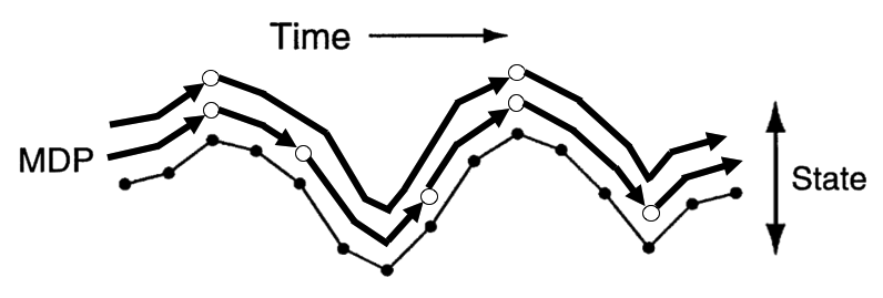
Figure 1: State trajectories over a three-level hierarchy of options. Open circles represent SMDP decision points while filled circles are primitive steps within an option. The low level options are temporally extended over primitive actions, and high level options are even further extended.

Work on learning with temporal abstraction is motivated by two key potential benefits over learning with primitive actions: long term credit assignment and exploration. Learning only at the primitive action level or even with low levels of abstraction slows down learning, because agents must learn longer sequences of actions to achieve the desired behavior. This frustrates the process of learning in environments with sparse rewards. In contrast, agents that learn a high level decomposition of sub-tasks are able to explore the environment more effectively by exploring in the abstract action space rather than the primitive action space. While the recently proposed deliberation cost [9] can be used as a margin that effectively controls how temporally extended options are, the standard two-level version of the option-critic framework is still ill-equipped to learn complex tasks that require sub-task decomposition at multiple quite different temporal resolutions of abstraction. In Figure 1 we depict how we overcome this obstacle to learn a deep hierarchy of options. The standard two-level option hierarchy constructs a Semi-Markov Decision Process (SMDP), where new options are chosen when temporally extended sequences of primitive actions are terminated. In our framework, we consider not just options and primitive actions, but also an arbitrarily deep hierarchy of lower level and higher level options. Higher level options represent a further temporally extended SMDP than the low level options below as they only have an opportunity to terminate when all lower level options terminate.

We will start by reviewing related research and by describing the seminal work we build upon in this paper that first derived policy gradient theorems for learning with primitive actions [42] and options [1]. We will then describe the core ideas of our approach, presenting hierarchical intra-option policy and termination gradient theorems. We leverage this new type of policy gradient learning to construct a hierarchical option-critic architecture, which generalizes the option-critic architecture to an arbitrarily deep hierarchy of options. Finally, we demonstrate the empirical benefit of this architecture over standard option-critic when applied to RL benchmarks. To the best of our knowledge, this is the first general purpose end-to-end approach for learning a deep hierarchy of options beyond two-levels in RL settings, scaling to very large domains at comparable efficiency.

2 Related Work

Our work is related to recent literature on learning to compose skills in RL. As an example, Sahni et al. [35] leverages a logic for combining pre-learned skills by learning an embedding to represent the combination of a skill and state. Unfortunately, their system relies on a pre-specified sub-task decomposition into skills. In [37], the authors propose to ground all goals in a natural language description space. Created descriptions can then be high level and express a sequence of goals. While these are interesting directions for further exploration, we will focus on a more general setting without provided natural language goal descriptions or sub-task decomposition information.

Our work is also related to methods that learn to decompose the problem over long time horizons. A prominent paradigm for this is Feudal Reinforcement Learning [5], which learns using manager and worker models. Theoretically, this can be extended to a deep hierarchy of managers and their managers as done in the original work for a hand designed decomposition of the state space. Much more recently, Vezhnevets et al. [44] showed the ability to successfully train a Feudal model end to end with deep neural networks for the Atari games. However, this has only been achieved for a two-level hierarchy (i.e. one manager and one worker). We can think of Feudal approaches as learning to decompose the problem with respect to the state space, while the options framework learns a temporal decomposition of the problem. Recent work [15] also breaks down the problem over a temporal hierarchy, but like [44] is based on learning a latent goal representation that modulates the policy behavior as opposed to options. Conceptually, options stress choosing among skill abstractions and Feudal approaches stress the achievement of certain kinds of states. Humans tend to use both of these kinds of reasoning when appropriate and we conjecture that a hybrid approach will likely win out in the end. Unfortunately, in the space available we feel that we cannot come to definitive conclusions about the precise nature of the differences and potential synergies of these approaches.

The concept of learning a hierarchy of options is not new. It is an obviously desirable extension of options envisioned in the original papers. However, actually learning a deep hierarchy of options end to end has received surprisingly little attention to date. Compositional planning where options select other options was first considered in [38]. The authors provided a generalization of value iteration to option models for multiple subgoals, leveraging explicit subgoals for options. Recently, Fox et al. [7] successfully trained a hierarchy of options end to end for imitation learning. Their approach leverages an EM based algorithm for recursive discovery of additional levels of the option hierarchy. Unfortunately, their approach is only applicable to imitation learning and not general purpose RL. We are the first to propose theorems along with a practical algorithm and architecture to train arbitrarily deep hierarchies of options end to end using policy gradients, maximizing the expected return.

3 Problem Setting and Notation

A Markov Decision Process (MDP) is defined with a set of states $\mathcal{S}$, a set of actions $\mathcal{A}$, a transition function $\mathcal{P}:\mathcal{S}\times\mathcal{A}\rightarrow(\mathcal{S}\rightarrow[0,1])$ and a reward function $r:\mathcal{S}\times\mathcal{A}\rightarrow\mathbb{R}$. We follow [1] and develop our ideas assuming discrete state and action sets, while our results extend to continuous spaces using usual measure-theoretic assumptions as demonstrated in our experiments. A policy is defined as a probability distribution over actions conditioned on states, $\pi:\mathcal{S}\rightarrow\mathcal{A}\rightarrow[0,1]$. The value function of a policy $\pi$ is the expected return $V_{\pi}(s)=\mathbb{E}_{\pi}[\sum_{t=0}^{\infty}\gamma^{t}r_{t+1}|s_{0}=s]$ with an action-value function of $Q_{\pi}(s,a)=\mathbb{E}_{\pi}[\sum_{t=0}^{\infty}\gamma^{t}r_{t+1}|s_{0}=s,a_{0}=a]$ where $\gamma\in[0,1)$ is the discount factor.

Policy gradient methods [42, 12] consider the problem of improving a policy by performing stochastic gradient descent to optimize a performance objective over a family of parametrized stochastic policies, $\pi_{\theta}$. The policy gradient theorem [42] provides the gradient of the discounted reward objective with respect to $\theta$ in a straightforward expression. The objective is defined with respect to a designated starting state $s_{0}:\rho(\theta,s_{0})=\mathbb{E}_{\pi_{\theta}}[\sum_{t=0}^{\infty}\gamma^{t}r_{t+1}|s_{0}]$. The policy gradient theorem shows that: $\frac{\partial\rho(\theta,s_{0})}{\partial\theta}=\sum_{s}\mu_{\pi_{\theta}}(s|s_{0})\sum_{a}\frac{\partial\pi_{\theta}(a|s)}{\partial\theta}Q_{\pi_{\theta}}(s,a)$, where $\mu_{\pi_{\theta}}(s|s_{0})=\sum_{t=0}^{\infty}\gamma^{t}P(s_{t}=s|s_{0})$ is the discounted weighting of the states along the trajectories starting from initial state $s_{0}$.

The options framework [41, 27] provides formalism for the idea of temporally extended actions. A Markovian option $o\in\Omega$ is a triple $(I_{o},\pi_{o},\beta_{o})$ where $I_{o}\subseteq S$ represents an initiation set, $\pi_{o}$ represents an intra-option policy, and $\beta_{o}:\mathcal{S}\rightarrow[0,1]$ represents a termination function. Like most option discovery algorithms, we assume that all options are available everywhere. MDPs with options become SMDPs [28] with an associated optimal value function over options $V^{*}_{\Omega}(s)$ and option-value function $Q^{*}_{\Omega}(s,o)$ [41, 27].

The option-critic architecture [1] utilizes a call-and-return option execution model. An agent picks option $o$ according to its policy over options $\pi_{\Omega}(o|s)$, then follows the intra-option policy $\pi(a|s,o)$ until termination (as determined by $\beta(s,o)$), which triggers a repetition of this procedure. Let $\pi_{\theta}(a|s,o)$ denote the intra-option policy of option $o$ parametrized by $\theta$ and $\beta_{\phi}(s,o)$ the termination function of $o$ parameterized by $\phi$. Like policy gradient methods, the option-critic architecture optimizes directly for the discounted return expected over trajectories starting at a designated state $s_{0}$ and option $o_{0}$: $\rho(\Omega,\theta,\phi,s_{0},o_{0})=\mathbb{E}_{\Omega,\pi_{\theta},\beta_{\phi}}[\sum_{t=0}^{\infty}\gamma^{t}r_{t+1}|s_{0},o_{0}]$. The option-value function is then:

$$Q_{\Omega}(s,o)=\sum_{a}\pi_{\theta}(a|s,o)Q_{U}(s,o,a),$$ (1)

where $Q_{U}:\mathcal{S}\times\Omega\times\mathcal{A}\rightarrow\mathbb{R}$ is the value of selecting an action given the context of a state-option pair:

$$Q_{U}(s,o,a)=r(s,a)+\gamma\sum_{s^{\prime}}P(s^{\prime}|s,a)U(s^{\prime},o).$$ (2)

The $(s,o)$ pairs define an augmented state space [16]. The option-critic architecture instead leverages the function $U:\Omega\times\mathcal{S}\rightarrow\mathbb{R}$ which is called the option-value function upon arrival [41]. The value of selecting option $o$ upon entering state $s^{\prime}$ is:

$$U(s^{\prime},o)=(1-\beta_{\phi}(s^{\prime},o))Q_{\Omega}(s^{\prime},o)+\beta_{\phi}(s^{\prime},o)V_{\Omega}(s^{\prime}).$$ (3)

For notation clarity, we omit $\theta$ and $\phi$ which $Q_{U}$ and $U$ both depend on. The intra-option policy gradient theorem results from taking the derivative of the expected discounted return with respect to the intra-option policy parameters $\theta$ and defines the update rule for the intra-option policy:

$$\frac{\partial Q_{\Omega}(s_{0},o_{0})}{\partial\theta}=\sum_{s,o}\mu_{\Omega}(s,o|s_{0},o_{0})\sum_{a}\frac{\partial\pi_{\theta}(a|s,o)}{\partial\theta}Q_{U}(s,o,a).$$ (4)

where $\mu_{\Omega}$ is the discounted weighting of $(s,o)$ along trajectories originating from $(s_{0},o_{0}):\mu_{\Omega}(s,o|s_{0},o_{0})=\sum_{t=0}^{\infty}\gamma^{t}P(s_{t}=s,o_{t}=o|s_{0},o_{0})$. The termination gradient theorem results from taking the derivative of the expected discounted return with respect to the termination policy parameters $\phi$ and defines the update rule for the termination policy for the initial condition $(s_{1},o_{0})$:

$$\frac{\partial Q_{\Omega}(s,o)}{\partial\phi}=\sum_{a}\pi_{\theta}(a|s,o)\sum_{s^{\prime}}\gamma P(s^{\prime}|s,a)\frac{\partial U(s^{\prime},o)}{\partial\phi},$$ (5)

$$\frac{\partial U(s_{1},o_{0})}{\partial\phi}=-\sum_{s^{\prime},o}\mu_{\Omega}(s^{\prime},o|s_{1},o_{o})\frac{\partial\beta_{\phi}(s^{\prime},o)}{\partial\phi}A_{\Omega}(s^{\prime},o),$$ (6)

where $\mu_{\Omega}$ is now the discounted weighting of $(s,o)$ from $(s_{1},o_{0}):\mu_{\Omega}(s,o|s_{1},o_{0})=\sum_{t=0}^{\infty}\gamma^{t}P(s_{t+1}=s,o_{t}=o|s_{1},o_{0})$. $A_{\Omega}$ is the advantage function over options: $A_{\Omega}(s^{\prime},o)=Q_{\Omega}(s^{\prime},o)-V_{\Omega}(s^{\prime})$.

4 Learning Options with Arbitrary Levels of Abstraction

Notation: As it makes our equations much clearer and more condensed we adopt the notation $x^{i:i+j}=x^{i},...,x^{i+j}$. This implies that $x^{i:i+j}$ denotes a list of variables in the range of $i$ through $i+j$.

The hierarchical options framework that we introduce in this work considers an agent that learns using an $N$ level hierarchy of policies, termination functions, and value functions. Our goal is to extend the ideas of the option-critic architecture in such a way that our framework simplifies to policy gradient based learning when $N=1$ and option-critic learning when $N=2$. At each hierarchical level above the lowest primitive action level policy, we consider an available set of options $\Omega^{1:N-1}$ that is a subset of the total set of available options $\Omega$. This way we keep our view of the possible available options at each level very broad. On one extreme, each hierarchical level may get its own unique set of options and on the other extreme each hierarchical level may share the same set of options. We present a diagram of our proposed architecture in Figure 2.

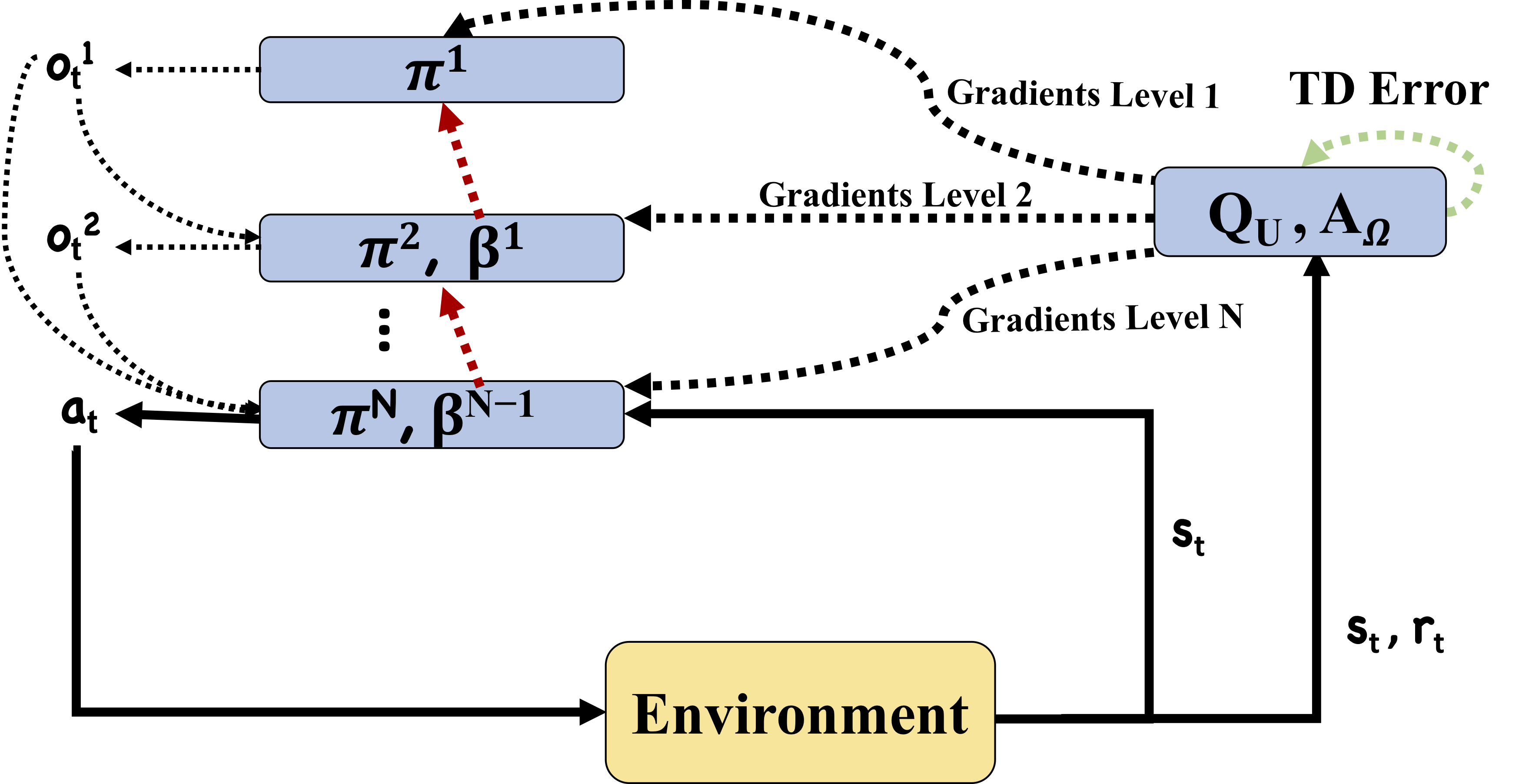
Figure 2: A diagram describing our proposed hierarchical option-critic architecture. Dotted lines represent processes within the agent while solid lines represent processes within the environment. Option selection is top down through the hierarchy and option termination is bottom up (represented with red dotted lines).

We denote $\pi_{\theta^{1}}^{1}(o^{1}|s)$ as the policy over the most abstract options in the hierarchy $o^{1}\in\Omega_{1}$ given the state $s$. For example, $\pi^{1}=\pi_{\Omega}$ from our discussion of the option-critic architecture. Once $o^{1}$ is chosen with policy $\pi^{1}$, then we go to policy $\pi_{\theta^{2}}^{2}(o^{2}|s,o^{1})$, which is the next highest level policy, to select $o^{2}\in\Omega_{2}$ conditioning it on both the current state $s$ and the selected highest level option $o^{1}$. This process continues on in the same fashion stepping down to policies at lower levels of abstraction conditioned on the augmented state space considering all selected higher level options until we reach policy $\pi_{\theta^{N}}^{N}(a|s,o^{1:N-1})$. $\pi^{N}$ is the lowest level policy and it finally selects over the primitive action space conditioned on all of the selected options.

Each level of the option hierarchy has a complimentary termination function $\beta_{\phi^{1}}^{1}(s,o^{1}),...,\beta_{\phi^{N-1}}^{N-1}(s,o^{1:N-1})$ that governs the termination pattern of the selected option at that level. We adopt a bottom up termination strategy where high level options only have an opportunity to terminate when all of the lower level options have terminated first. For example, $o_{t}^{N-2}$ cannot terminate until $o_{t}^{N-1}$ terminates at which point we can assess $\beta_{\phi^{N-2}}^{N-2}(s,o^{1:N-2})$ to see whether $o_{t}^{N-2}$ terminates. If it did terminate, this would allow $o_{t}^{N-3}$ the opportunity to asses if it should terminate and so on. This condition ensures that higher level options will be more temporally extended than their lower level option building blocks, which is a key motivation of this work.

The final key component of our system is the value function over the augmented state space at each level of abstraction. To enable comprehensive reasoning about the policies at each level of the option hierarchy, we need to maintain value functions that consider the state and every possible combination of active options and actions $V_{\Omega}(s),Q_{\Omega}(s,o^{1}),...,Q_{\Omega}(s,o^{1:N-1},a)$. These value functions collectively serve as the critic in our analogy to the actor-critic and option-critic training paradigms.

4.1 Generalizing the Option Value Function to N Hierarchical Levels

Like policy gradient methods and option-critic, the hierarchical options framework optimizes directly for the discounted return expected over all trajectories starting at a state $s_{0}$ with active options $o_{0}^{1:N-1}$:

$$\begin{split}\rho(\Omega^{1:N-1},\theta^{1:N},\phi^{1:N-1},s_{0},o_{0}^{1:N-1})=\mathbb{E}_{\Omega^{1:N-1},\pi^{1:N}_{\theta},\beta^{1:N-1}_{\phi}}[\sum_{t=0}^{\infty}\gamma^{t}r_{t+1}|s_{0},o_{0}^{1:N-1}]\end{split}$$ (7)

This return depends on the policies and termination functions at each level of abstraction. We now consider the option value function for understanding reasoning about an option $o^{\ell}$ at level $1\leq\ell\leq N$ based on the augmented state space $(s,o^{1:\ell-1})$:

$$Q_{\Omega}(s,o^{1:\ell-1})=\sum_{o^{\ell}}\pi^{\ell}_{\theta^{\ell}}(o^{\ell}|s,o^{1:\ell-1})Q_{\Omega}(s,o^{1:\ell})$$ (8)

Note that in order to simplify our notation we write $o^{\ell}$ as referring to both abstract and primitive actions. As a result, $o^{N}$ is equivalent to $a$, leveraging the primitive action space $\mathcal{A}$. Extending the meaning of $Q_{U}$ from [1], we define the corresponding value of executing an option in the presence of the currently active higher level options by integrating out the lower level options:

$$\begin{split}Q_{U}(s,o^{1:\ell})\!=\!\sum_{o^{N}}\!\!...\!\!\sum_{o^{\ell+1}}\!\prod_{j=\ell+1}^{N}\!\!\!\!\pi^{j}(o^{j}|s,o^{1:j-\!1})[r(s,\!o^{N})\!+\!\gamma\!\sum_{s^{\prime}}\!P(s^{\prime}|s,o^{N})U(s^{\prime},o^{1:\ell})].\end{split}$$ (9)

The hierarchical option value function upon arrival $U$ with augmented state $(s,o^{1:\ell})$ is defined as:

$$\begin{split}U(s^{\prime},o^{1:\ell})=\underbrace{(1-\beta_{\phi^{N-1}}^{N-1}(s^{\prime},o^{1:N-1}))Q_{\Omega}(s^{\prime},o^{1:N-1})}_{\text{none terminate ($N\geq 1$)}}+\underbrace{V_{\Omega}(s^{\prime})\prod_{j=N-1}^{1}\beta_{\phi^{j}}^{j}(s^{\prime},o^{1:j})}_{\text{all options terminate ($N\geq 2$)}}+\\ \underbrace{Q_{\Omega}(s^{\prime},o^{1:\ell})\sum_{q=N-1}^{\ell+1}(1-\beta_{\phi^{q-1}}^{q-1}(s^{\prime},o^{1:q-1}))\prod_{z=N-1}^{q}\beta_{\phi^{z}}^{z}(s^{\prime},o^{1:z})}_{\text{only lower level options terminate ($N\geq 3$)}}+\\ \underbrace{\sum_{i=1}^{\ell-1}(1-\beta_{\phi^{i}}^{i}(s^{\prime},o^{1:i}))Q_{\Omega}(s^{\prime},o^{1:i})\prod_{k=i+1}^{N-1}\beta_{\phi^{k}}^{k}(s^{\prime},o^{1:k})}_{\text{some relevant higher level options terminate ($N\geq 3$)}}].\end{split}$$ (10)

We explain the derivation of this equation in the Appendix A.1. Finally, before we can extend the policy gradient theorem, we must establish the Markov chain along which we can measure performance for options with $N$ levels of abstraction. This is derived in the Appendix A.2.

4.2 Generalizing the Intra-option Policy Gradient Theorem

We can think of actor-critic architectures, generalizing to the option-critic architecture as well, as pairing a critic with each actor network so that the critic has additional information about the value of the actor’s actions that can be used to improve the actor’s learning. However, this is derived by taking gradients with respect to the parameters of the policy while optimizing for the expected discounted return. The discounted return is approximated by a critic (i.e. value function) with the same augmented state-space as the policy being optimized for. As examples, an actor-critic policy $\pi(a|s)$ is optimized by taking the derivative of its parameters with respect to $V_{\pi}(s)$ [42] and an option-critic policy $\pi(a|s,o)$ is optimized by taking the derivative of its parameters with respect to $Q_{\Omega}(s,o)$ [1]. The intra-option policy gradient theorem [1] is an important contribution, outlining how to optimize for a policy that is also associated with a termination function. As the policy over options in that work never terminates, it does not need a special training methodology and the option-critic architecture allows the practitioner to pick their own method of learning the policy over options while using Q Learning as an example in their experiments. We do the same for our highest level policy $\pi^{1}$ that also never terminates. For all other policies $\pi^{2:N}$ we perform a generalization of actor-critic learning by providing a critic at each level and guiding gradients using the appropriate critic.

We now seek to generalize the intra-option policy gradients theorem, deriving the update rule for a policy at an arbitrary level of abstraction $\pi^{\ell}$ by taking the gradient with respect to $\theta^{\ell}$ using the value function with the same augmented state space $Q_{\Omega}(s,o^{1:\ell-1})$. Substituting from equation (8) we find:

$$\frac{\partial Q_{\Omega}(s,o^{1:\ell-1})}{\partial\theta^{\ell}}=\frac{\partial}{\partial\theta^{\ell}}\sum_{o^{\ell}}\pi^{\ell}_{\theta^{\ell}}(o^{\ell}|s,o^{1:\ell-1})Q_{U}(s,o^{1:\ell}).$$ (11)

Theorem 1 (Hierarchical Intra-option Policy Gradient Theorem). Given an $N$ level hierarchical set of Markov options with stochastic intra-option policies differentiable in their parameters $\theta^{\ell}$ governing each policy $\pi^{\ell}$, the gradient of the expected discounted return with respect to $\theta^{\ell}$ and initial conditions $(s_{0},o_{0}^{1:N-1})$ is:

$$\sum_{s,o^{1:\ell-1}}\mu_{\Omega}(s,o^{1:\ell-1}|s_{0},o_{0}^{1:\ell-1})\sum_{o^{\ell}}\frac{\partial\pi^{\ell}_{\theta^{\ell}}(o^{\ell}|s,o^{1:\ell-1})}{\partial\theta^{\ell}}Q_{U}(s,o^{1:\ell}),$$

where $\mu_{\Omega}$ is a discounted weighting of augmented state tuples along trajectories starting from $(s_{0},o_{0}^{1:N-1}):\mu_{\Omega}(s,o^{1:\ell-1}|s_{0},o_{0}^{1:\ell-1})=\sum_{t=0}^{\infty}\gamma^{t}P(s_{t}=s,o_{t}^{1:\ell-1}=o^{1:\ell-1}|s_{0},o_{0}^{1:\ell-1})$. A proof is in Appendix A.3.

4.3 Generalizing the Termination Gradient Theorem

We now turn our attention to computing gradients for the termination functions $\beta^{\ell}$ at each level, assumed to be stochastic and differentiable with respect to the associated parameters $\phi^{\ell}$.

$$\frac{\partial Q_{\Omega}(s,o^{1:\ell})}{\partial\phi^{\ell}}=\sum_{o^{N}}\!\!...\!\!\sum_{o^{\ell+1}}\!\prod_{j=\ell+1}^{N}\pi^{j}(o^{j}|s,o^{1:j-\!1})\!\gamma\!\sum_{s^{\prime}}\!P(s^{\prime}|s,o^{N})\frac{\partial U(s^{\prime},o^{1:\ell})}{\partial\phi^{\ell}}$$ (12)

Hence, the key quantity is the gradient of $U$. This is a natural consequence of call-and-return execution, where termination function quality can only be evaluated upon entering the next state.

Theorem 2 (Hierarchical Termination Gradient Theorem). Given an $N$ level hierarchical set of Markov options with stochastic termination functions differentiable in their parameters $\phi^{\ell}$ governing each function $\beta^{\ell}$, the gradient of the expected discounted return with respect to $\phi^{\ell}$ and initial conditions $(s_{1},o_{0}^{1:N-1})$ is:

$$-\sum_{s,o^{1:\ell}}\mu_{\Omega}(s,o^{1:N-1}|s_{1},o_{0}^{1:N-1})\prod_{i=\ell+1}^{N-1}\beta_{\phi^{i}}^{i}(s,o^{1:i})\frac{\partial\beta_{\phi^{\ell}}^{\ell}(s,o^{1:\ell})}{\partial\phi^{\ell}}A_{\Omega}(s,o^{1:\ell})$$

where $\mu_{\Omega}$ is a discounted weighting of augmented state tuples along trajectories starting from $(s_{1},o_{0}^{1:N-1}):\mu_{\Omega}(s,o^{1:\ell-1}|s_{1},o_{0}^{1:N-1})=\sum_{t=0}^{\infty}\gamma^{t}P(s_{t}=s,o_{t}^{1:\ell}=o^{1:\ell}|s_{1},o_{0}^{1:N-1})$. $A_{\Omega}$ is the generalized advantage function over a hierarchical set of options $A_{\Omega}(s^{\prime},o^{1:\ell})=Q_{\Omega}(s^{\prime},o^{1:\ell})-V_{\Omega}(s)[\prod_{j=\ell-1}^{1}\beta_{\phi^{j}}^{j}(s^{\prime},o^{1:j})]-\sum_{i=1}^{\ell-1}(1-\beta_{\phi^{i}}^{i}(s^{\prime},o^{1:i}))Q_{\Omega}(s^{\prime},o^{1:i})[\prod_{k=i+1}^{\ell-1}\beta_{\phi^{k}}^{k}(s^{\prime},o^{1:k})]$. $A_{\Omega}$ compares the advantage of not terminating the current option with a probability weighted expectation based on the likelihood that higher level options also terminate. In [1] this expression was simple as there was not a hierarchy of higher level termination functions to consider. A proof is in Appendix A.4.

It is interesting to see the emergence of an advantage function as a natural consequence of the derivation. As in [1] where this kind of relationship also appears, the advantage function gives the theorem an intuitive interpretation. When the option choice is sub-optimal at level $\ell$ with respect to the expected value of terminating option $\ell$, the advantage function is negative and increases the odds of terminating that option. A new concept, not paralleled in the option-critic derivation, is the inclusion of a $\prod_{i=\ell+1}^{N-1}\beta_{\phi^{i}}^{i}(s,o^{1:i})$ multiplicative factor. This can be interpreted as discounting gradients by the likelihood of this termination function being assessed as $\beta^{\ell}$ is only used if all lower level options terminate. This is a natural consequence of multi-level call-and-return execution.

5 Experiments

We would now like to empirically validate the efficacy of our proposed hierarchical option-critic (HOC) model. We achieve this by exploring benchmarks in the tabular and non-linear function approximation settings. In each case we implement an agent that is restricted to primitive actions (i.e. $N=1$), an agent that leverages the option-critic (OC) architecture (i.e. $N=2$), and an agent with the HOC architecture at level of abstraction $N=3$. We will demonstrate that complex RL problems may be more easily learned using beyond two levels of abstraction and that the HOC architecture can successfully facilitate this level of learning using data from scratch.

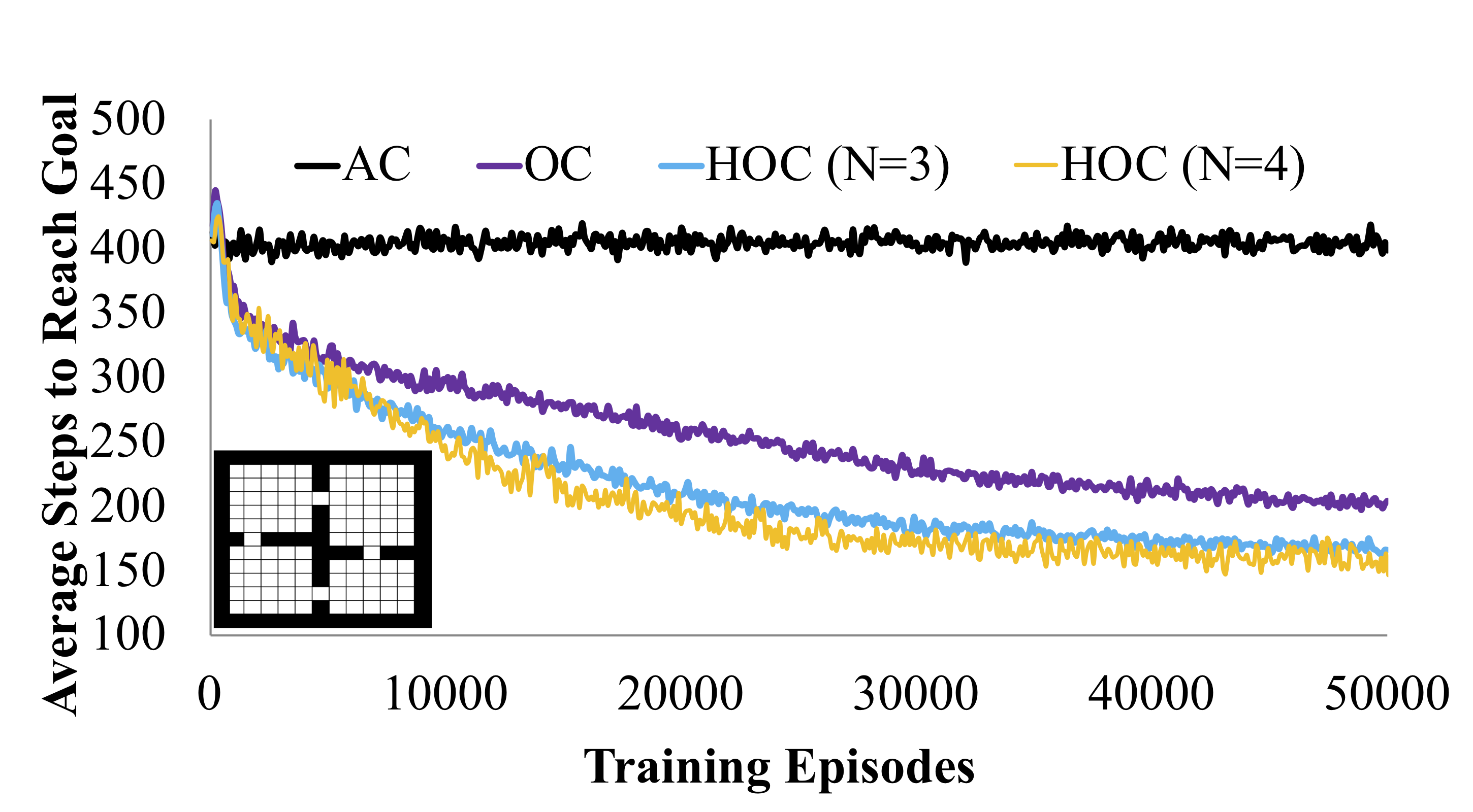
Figure 3: Learning performance as a function of the abstraction level for a nonstationary four rooms domain where the goal location changes every episode.

For our tabular architectures, we followed protocol from [1] and chose to parametrize the intra-option policies with softmax distributions and the terminations with sigmoid functions. The policy over options was learned using intra-option Q-learning. We also implemented primitive actor-critic (AC) using a softmax policy. For the non-linear function approximation setting, we trained our agents using A3C [25]. Our primitive action agents conduct A3C training using a convolutional network when there is image input followed by an LSTM to contextualize the state. This way we ensure that benefits seen from options are orthogonal to those seen from these common neural network building blocks. We follow [9] to extend A3C to the Asynchronous Advantage Option-Critic (A2OC) and Asynchronous Advantage Hierarchical Option-Critic architectures (A2HOC). We include detailed algorithm descriptions for all of our experiments in Appendix B. We also conducted hyperparameter optimization that is summarized along with detail on experimental protocol in Appendix B. In all of our experiments, we made sure that the two-level OC architecture had access to more total options than the three level alternative and that the three level architecture did not include any additional hyperparameters. This ensures that empirical gains are the result of increasingly abstract options.

5.1 Tabular Learning Challenge Problems

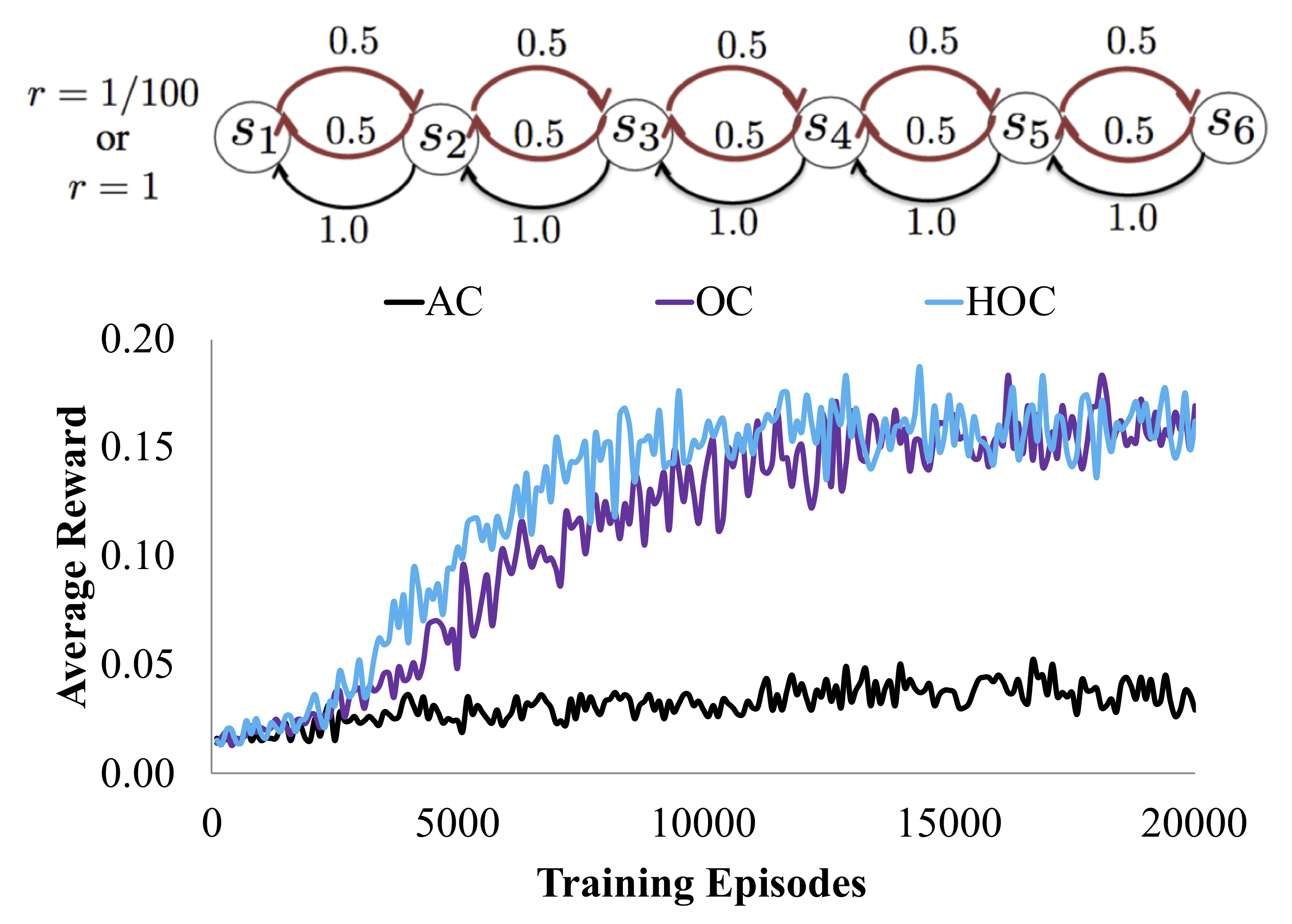
Figure 4: The diagram, from [14], details the stochastic decision process challenge problem. The chart compares learning performance across abstract reasoning levels.

Exploring four rooms: We first consider a navigation task in the four-rooms domain [41]. Our goal is to evaluate the ability of a set of options learned fully autonomously to learn an efficient exploration policy within the environment. The initial state and the goal state are drawn uniformly from all open non-wall cells every episode. This setting is highly non-stationary, since the goal changes every episode. Primitive movements can fail with probability $\frac{1}{3}$, in which case the agent transitions randomly to one of the empty adjacent cells. The reward is +1 at the goal and 0 otherwise. In Figure 3 we report the average number of steps taken in the last 100 episodes every 100 episodes, reporting the average of 50 runs with different random seeds for each algorithm. We can clearly see that reasoning with higher levels of abstraction is critical to achieving a good exploration policy and that reasoning with three levels of abstraction results in better sample efficient learning than reasoning with two levels of abstraction. For this experiment we explore four levels of abstraction as well, but unfortunately there seem to be diminishing returns at least for this tabular setting.

Discrete stochastic decision process: Next, we consider a hierarchical RL challenge problem as explored in [14] with a stochastic decision process where the reward depends on the history of visited states in addition to the current state. There are 6 possible states and the agent always starts at $s_{2}$. The agent moves left deterministically when it chooses left action; but the action right only succeeds half of the time, resulting in a left move otherwise. The terminal state is $s_{1}$ and the agent receives a reward of 1 when it first visits $s_{6}$ and then $s_{1}$. The reward for going to $s_{1}$ without visiting $s_{6}$ is 0.01. In Figure 4 we report the average reward over the last 100 episodes every 100 episodes, considering 10 runs with different random seeds for each algorithm. Reasoning with higher levels of abstraction is again critical to performing well at this task with reasonable sample efficiency. Both OC learning and HOC learning converge to a high quality solution surpassing performance obtained in [14]. However, it seems that learning converges faster with three levels of abstractions than it does with just two.

5.2 Deep Function Approximation Problems

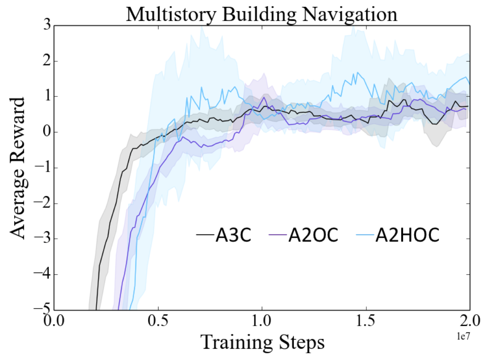
Figure 5: Building navigation learning performance across abstract reasoning levels.

Multistory building navigation: For an intuitive look at higher level reasoning, we consider the four rooms problem in a partially observed setting with an 11x17 grid at each level of a seven level building. The agent has a receptive field size of 3 in both directions, so observations for the agent are 9-dimension feature vectors with 0 in empty spots, 1 where there is a wall, 0.25 if there are stairs, or 0.5 if there is a goal location. The stairwells in the north east corner of the floor lead upstairs to the south west corner of the next floor up. Stairs in the south west corner of the floor lead down to the north east corner of the floor below. Agents start in a random location in the basement (which has no south west stairwell) and must navigate to the roof (which has no north east stairwell) to find the goal in a random location. The reward is +10 for finding the goal and -0.1 for hitting a wall. This task could seemingly benefit from abstraction such as a composition of sub-policies to get to the stairs at each intermediate level. We report the rolling mean and standard deviation of the reward. In Figure 5 we see a qualitative difference between the policies learned with three levels of abstraction which has high variance, but fairly often finds the goal location and those learned with less abstraction. A2OC and A3C are hovering around zero reward, which is equivalent to just learning a policy that does not run into walls.

Architecture	Clipped Reward
A3C	8.43 $\pm$ 2.29
A2OC	10.56 $\pm$0.49
A2HOC	13.12 $\pm$1.46

Table 1: Average clipped reward per episode over 5 runs on 21 Atari games.

Learning many Atari games with one model: We finally consider application of the HOC to the Atari games [2]. Evaluation protocols for the Atari games are famously inconsistent [18], so to ensure for fair comparisons we implement apples to apples versions of our baseline architectures deployed with the same code-base and environment settings. We put our models to the test and consider a very challenging setting [36] where a single agent attempts to learn many Atari games at the same time. Our agents attempt to learn 21 Atari games simultaneously, matching the largest previous multi-task setting on Atari [36]. Our tasks are hand picked to fall into three categories of related games each with 7 games represented. The first category is games that include maze style navigation (e.g. MsPacman), the second category is mostly fully observable shooter games (e.g. SpaceInvaders), and the final category is partially observable shooter games (e.g. BattleZone). We train each agent by always sampling the game with the least training frames after each episode, ensuring the games are sampled very evenly throughout training. We also clip rewards to allow for equal learning rates across tasks [24]. We train each game for 10 million frames (210 million total) and report statistics on the clipped reward achieved by each agent when evaluating the policy without learning for another 3 million frames on each game across 5 separate training runs. As our main metric, we report the summary of how each multi-task agent maximizes its reward in Table 1. While all agents struggle in this difficult setting, HOC is better able to exploit commonalities across games using fewer parameters and policies.

Analysis of Learned Options: An advantage of the multi-task setting is it allows for a degree of quantitative interpretability regarding when and how options are used. We report characteristics of the agents with median performance during the evaluation period. A2OC with 16 options uses 5 options the bulk of the time with the rest of the time largely split among another 6 options (Figure 6). The average number of time steps between switching options has a pretty narrow range across games falling between 3.4 (Solaris) and 5.5 (MsPacman). In contrast, A2HOC with three options at each branch of the hierarchy learns to switch options at a rich range of temporal resolutions depending on the game. The high level options vary between an average of 3.2 (BeamRider) and 9.7 (Tutankham) steps before switching. Meanwhile, the low level options vary between an average of 1.5 (Alien) and 7.8 (Tutankham) steps before switching. In Appendix B.4 we provide additional details about the average duration before switching options for each game. In Figure 7 we can see that the most used options for HOC are distributed pretty evenly across a number of games, while OC tends to specialize its options on a smaller number of games. In fact, the average share of usage dominated by a single game for the top 7 most used options is 40.9% for OC and only 14.7% for HOC. Additionally, we can see that a hierarchy of options imposes structure in the space of options. For example, when $o^{1}=1$ or $o^{1}=2$ the low level options tend to focus on different situations within the same games.

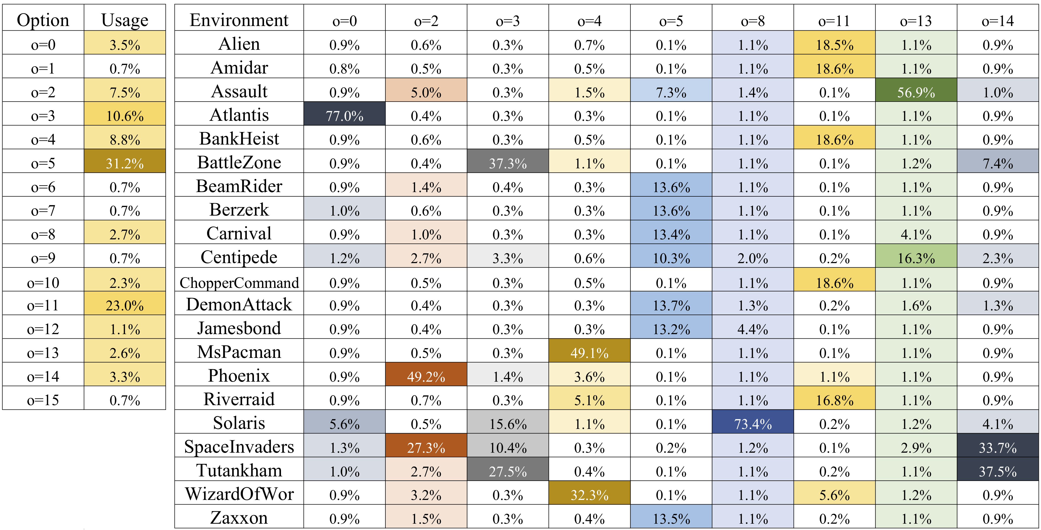
Figure 6: Option usage (left) and specialization across Atari games for the top 9 most used options (right) of a 16 option Option-Critic architecture trained in the many task learning setting.

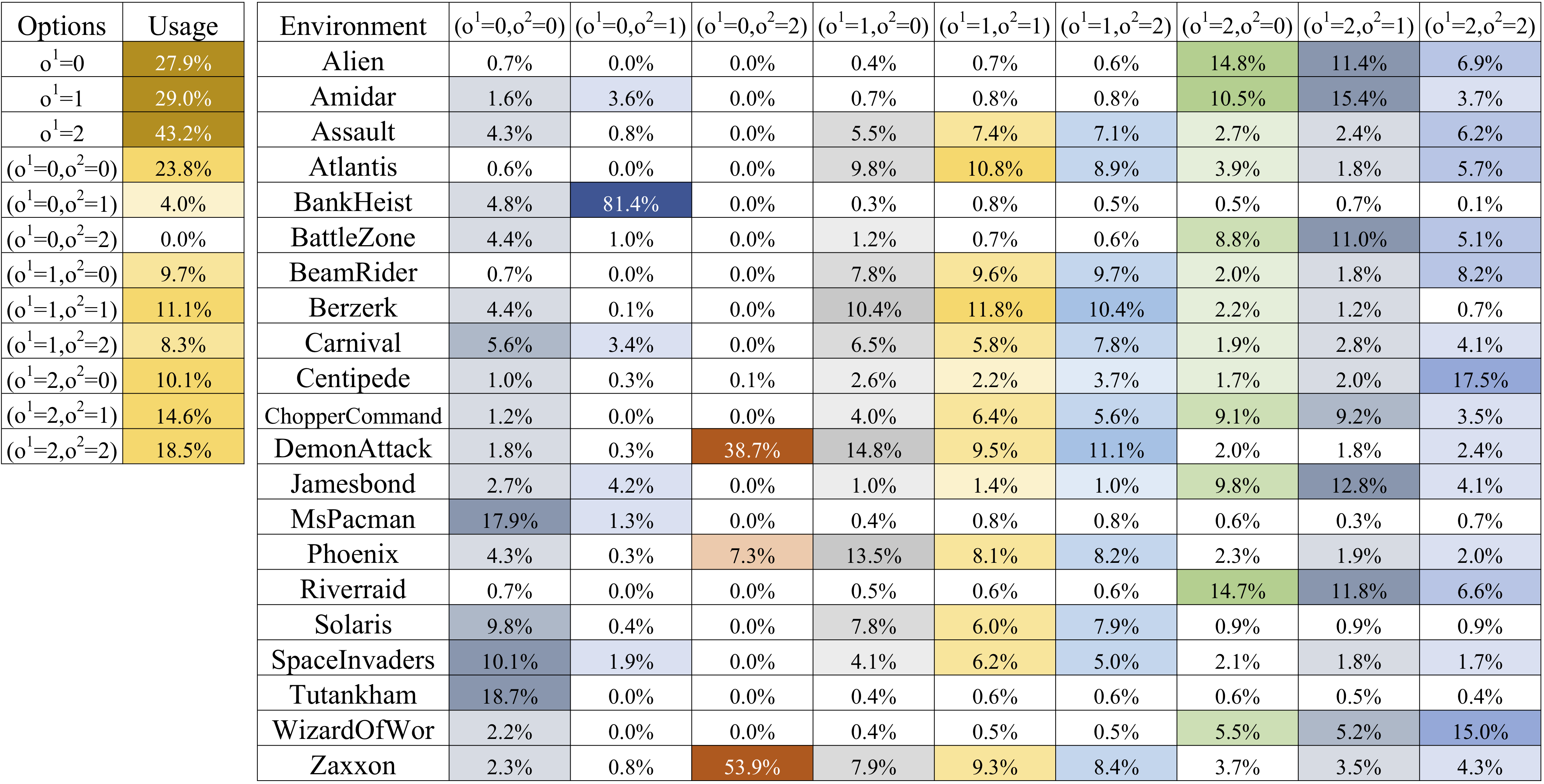
Figure 7: Option usage (left) and specialization across Atari games (right) of a Hierarchical Option-Critic architecture with $N=3$ and 3 options at each layer trained in the many task learning setting.

6 Conclusion

In this work we propose the first policy gradient theorems to optimize an arbitrarily deep hierarchy of options to maximize the expected discounted return. Moreover, we have proposed a particular hierarchical option-critic architecture that is the first general purpose reinforcement learning architecture to successfully learn options from data with more than two abstraction levels. We have conducted extensive empirical evaluation in the tabular and deep non-linear function approximation settings. In all cases we found that, for significantly complex problems, reasoning with more than two levels of abstraction can be beneficial for learning. While the performance of the hierarchical option-critic architecture is impressive, we envision our proposed policy gradient theorems eventually transcending it in overall impact. Although the architectures we explore in this paper have a fixed structure and fixed depth of abstraction for simplicity, the underlying theorems can also guide learning for much more dynamic architectures that we hope to explore in future work.

Appendix A Derivation of Generalized Policy Gradient and Termination Gradient Theorems

A.1 The Derivation of U

To help explain the meaning and derivation of equation (10), we separate the expression into four primary terms. The first term is applicable for $N\geq 1$ and represents the expected return from cases where no options terminate. The second term is applicable for $N\geq 2$ and represents the expected return from cases where every option terminates. The third and fourth terms are applicable for $N\geq 3$ and represent the expected return from cases where some options terminate.

We will first discuss how to estimate the return when there are no terminated options. In this case we simply use our estimate of the value of the current state following the current options if there are any. As we are computing the expectation, we also multiply this term by its likelihood of happening which is equal to the probability that the lowest level option policy does not terminate. When $N=1$ we can consider the termination probability of the current policy as zero and the current option context to be empty. As such, we estimate the value function upon arrival as $V_{\Omega}(s)$ as we do for actor-critic policy gradients.

Next we turn our attention to estimating the return when all options are terminated. This can be approximated using our estimate of the return given the state $V_{\Omega}(s)$. The likelihood of this happening is equal to the conditional likelihood of options terminating at every level of abstraction we are modeling. When $N=2$, equation (10) simplifies to equation (3). This expression is precisely the option value function upon arrival of the option-critic framework derived in [1].

The final quantity we will estimate bridges the gap to cases where only some options terminate. This situation has not been explored by other work on option learning as it only arises for situations with at least $N=3$ hierarchical levels of planning. The case where some (but not all) options terminate arises when a series of low level options terminate while a high level option does not terminate. For a given level of abstraction, we can analyze the likelihood that at each level the lower level options terminate while the current does not. In such a case, we multiply this likelihood by the value one level more abstract than the current option hierarchy level. For convenience in our derivation, we split our notation for this quantity into two separate terms accounting explicitly for the case when only lower level options terminate.

A.2 Generalized Markov Chain and Augmented Process

We must establish the Markov chain along which we can measure performance for options with $N$ levels of abstraction. The natural approach is to consider the chain defined in the augmented state space because state and active option based tuples now play the role of regular states in a usual Markov chain. If options $o_{t}^{1:N-1}$ have been initiated or are executing at time $t$ in state $s_{t}$, then the probability of transitioning to $(s_{t+1},o_{t+1}^{1:\ell-1})$ in one step is:

$$\begin{split}P(s_{t+1},o_{t+1}^{1:\ell-1}|s_{t},o_{t}^{1:N-1})=\sum_{o_{t}^{N}}\pi_{\theta^{N}}^{N}(o_{t}^{N}|s_{t},o_{t}^{1:N-1})P(s_{t+1}|s_{t},o_{t}^{N})[\\ \underbrace{(1-\beta_{\phi^{N-1}}^{N-1}(s_{t+1},o_{t}^{1:N-1}))\textbf{1}_{o_{t+1}^{1:\ell-1}=o_{t}^{1:\ell-1}}}_{\text{none terminate}}+\\ \underbrace{\sum_{q=N-1}^{\ell}(1-\beta_{\phi^{q-1}}^{q-1}(s_{t+1},o_{t}^{1:q-1}))\prod_{z=N-1}^{q}\beta_{\phi^{z}}^{z}(s_{t+1},o_{t}^{1:z})\textbf{1}_{o_{t+1}^{1:\ell-1}=o_{t}^{1:\ell-1}}}_{\text{only lower level options terminate}}+\\ \underbrace{\prod_{j=N-1}^{1}\beta_{\phi^{j}}^{j}(s_{t+1},o_{t}^{1:j})\prod_{v=\ell-1}^{1}\pi_{\theta^{v}}^{v}(o_{t+1}^{v}|s_{t+1},o_{t}^{1:v-1})}_{\text{all options terminate}}+\\ \underbrace{\sum_{i=1}^{\ell-2}(1-\beta_{\phi^{i}}^{i}(s_{t+1},o_{t}^{1:i}))\prod_{k=i+1}^{N-1}\beta_{\phi^{k}}^{k}(s_{t+1},o_{t}^{1:k})\prod_{p=i+1}^{\ell-1}\pi_{\theta^{p}}^{p}(o_{t+1}^{p}|s_{t+1},o_{t}^{1:p-1})}_{\text{some relevant higher level options terminate}}].\end{split}$$ (13)

where primitive actions are $o^{N}$. Like the Markov chain derived for the option critic architecture [1], the process given by equation (13) is homogeneous. Additionally, when options are available at every state, the process is ergodic with the existance of a unique stationary distribution over the augmented state space tuples.

We continue by presenting an extension of results about augmented processes used for derivation of learning algorithms in [1] to an option hierarchy with $N$ levels of abstraction. If options $o^{1:N-1}_{t}$ have been initiated or are executing at time $t$, then the discounted probability of transitioning to $(s_{t+1},o^{1:\ell-1}_{t+1})$ where $\ell\leq N$ is:

$$\begin{split}P_{\gamma}^{(1)}(s_{t+1},o_{t+1}^{1:\ell-1}|s_{t},o_{t}^{1:N-1})=\sum_{o_{t}^{N}}\pi_{\theta^{N}}^{N}(o_{t}^{N}|s_{t},o_{t}^{1:N-1})\gamma P(s_{t+1}|s_{t},o_{t}^{N})[\\ \underbrace{(1-\beta_{\phi^{N-1}}^{N-1}(s_{t+1},o_{t}^{1:N-1}))\textbf{1}_{o_{t+1}^{1:\ell-1}=o_{t}^{1:\ell-1}}}_{\text{none terminate}}+\\ \underbrace{\sum_{q=N-1}^{\ell}(1-\beta_{\phi^{q-1}}^{q-1}(s_{t+1},o_{t}^{1:q-1}))\prod_{z=N-1}^{q}\beta_{\phi^{z}}^{z}(s_{t+1},o_{t}^{1:z})\textbf{1}_{o_{t+1}^{1:\ell-1}=o_{t}^{1:\ell-1}}}_{\text{only lower level options terminate}}+\\ \underbrace{\prod_{j=N-1}^{1}\beta_{\phi^{j}}^{j}(s_{t+1},o_{t}^{1:j})\prod_{v=\ell-1}^{1}\pi_{\theta^{v}}^{v}(o_{t+1}^{v}|s_{t+1},o_{t}^{1:v-1})}_{\text{all options terminate}}+\\ \underbrace{\sum_{i=1}^{\ell-2}(1-\beta_{\phi^{i}}^{i}(s_{t+1},o_{t}^{1:i}))\prod_{k=i+1}^{N-1}\beta_{\phi^{k}}^{k}(s_{t+1},o_{t}^{1:k})\prod_{p=i+1}^{\ell-1}\pi_{\theta^{p}}^{p}(o_{t+1}^{p}|s_{t+1},o_{t}^{1:p-1})}_{\text{some relevant higher level options terminate}}].\\ \end{split}$$ (14)

As such, when we condition the process from $(s_{t},o^{1:N-1}_{t-1})$, the discounted probability of transitioning to $(s_{t+1},o^{1:\ell-1}_{t})$ is:

$$\begin{split}P_{\gamma}^{(1)}(s_{t+1},o_{t}^{1:\ell-1}|s_{t},o_{t-1}^{1:N-1})=\sum_{o_{t}^{N}}\pi_{\theta^{N}}^{N}(o_{t}^{N}|s_{t},o_{t}^{1:N-1})\gamma P(s_{t+1}|s_{t},o_{t}^{N})[\\ \underbrace{(1-\beta_{\phi^{N-1}}^{N-1}(s_{t+1},o_{t-1}^{1:N-1}))\textbf{1}_{o_{t}^{1:\ell-1}=o_{t-1}^{1:\ell-1}}}_{\text{none terminate}}+\\ \underbrace{\sum_{q=N-1}^{\ell}(1-\beta_{\phi^{q-1}}^{q-1}(s_{t+1},o_{t-1}^{1:q-1}))\prod_{z=N-1}^{q}\beta_{\phi^{z}}^{z}(s_{t+1},o_{1:t-1}^{z})\textbf{1}_{o_{t}^{1:\ell-1}=o_{t-1}^{1:\ell-1}}}_{\text{only lower level options terminate}}+\\ \underbrace{\prod_{j=N-1}^{1}\beta_{\phi^{j}}^{j}(s_{t+1},o_{t-1}^{1:j})\prod_{v=\ell-1}^{1}\pi_{\theta^{v}}^{v}(o_{t}^{v}|s_{t+1},o_{t-1}^{1:v-1})}_{\text{all options terminate}}+\\ \underbrace{\sum_{i=1}^{\ell-2}(1-\beta_{\phi^{i}}^{i}(s_{t+1},o_{t-1}^{1:i}))\prod_{k=i+1}^{N-1}\beta_{\phi^{k}}^{k}(s_{t+1},o_{t-1}^{1:k})\prod_{p=i+1}^{\ell-1}\pi_{\theta^{p}}^{p}(o_{t}^{p}|s_{t+1},o_{t-1}^{1:p-1})}_{\text{some relevant higher level options terminate}}].\\ \end{split}$$ (15)

This definition will be very useful later for our derivation of the hierarchical intra-option policy gradient. However, for the derivation of the hierarchical termination gradient theorem we should reformulate the discounted probability of transitioning to $(s_{t+1},o^{1:\ell}_{t})$ from the view of the termination policy at abstraction level $\ell$ explicitly separating out terms that depend on $\phi^{\ell}$:

$$\begin{split}P_{\gamma}^{(1)}(s_{t+1},o_{t}^{1:\ell}|s_{t},o_{t-1}^{1:N-1})=\sum_{o_{t}^{N}}\pi_{\theta^{N}}^{N}(o_{t}^{N}|s_{t},o_{t}^{1:N-1})\gamma P(s_{t+1}|s_{t},o_{t}^{N})[\\ \underbrace{(1-\beta_{\phi^{N-1}}^{N-1}(s_{t+1},o_{t-1}^{1:N-1}))\textbf{1}_{o_{t}^{1:\ell}=o_{t-1}^{1:\ell}}}_{\text{none terminate}}+\underbrace{\sum_{q=N-1}^{\ell+2}(1-\beta_{\phi^{q-1}}^{q-1}(s_{t+1},o_{t-1}^{1:q-1}))\prod_{z=N-1}^{q}\beta_{\phi^{z}}^{z}(s_{t+1},o_{t-1}^{1:z})\textbf{1}_{o_{t}^{1:\ell}=o_{t-1}^{1:\ell}}}_{\text{only lower level options terminate}}+\\ \underbrace{(1-\beta_{\phi^{\ell}}^{\ell}(s_{t+1},o_{t-1}^{1:\ell}))\prod_{z=N-1}^{\ell+1}\beta_{\phi^{z}}^{z}(s_{t+1},o_{t-1}^{1:z})\textbf{1}_{o_{t}^{1:\ell}=o_{t-1}^{1:\ell}}}_{\text{$\ell+1$ terminates and $\ell$ does not}}+\underbrace{\prod_{j=N-1}^{1}\beta_{\phi^{j}}^{j}(s_{t+1},o_{t-1}^{1:j})\prod_{v=\ell}^{1}\pi_{\theta^{v}}^{v}(o_{t}^{v}|s_{t+1},o_{t-1}^{1:v-1})}_{\text{all options terminate}}+\\ \underbrace{\sum_{i=1}^{\ell-1}(1-\beta_{\phi^{i}}^{i}(s_{t+1},o_{t-1}^{1:i}))\prod_{k=i+1}^{N-1}\beta_{\phi^{k}}^{k}(s_{t+1},o_{t-1}^{1:k})\prod_{p=i+1}^{\ell}\pi_{\theta^{p}}^{p}(o_{t}^{p}|s_{t+1},o_{t-1}^{1:p-1})}_{\text{some relevant higher level options terminate}}].\\ \end{split}$$ (16)

The $k$-step discounted probabilities can more generally be expressed recursively:

$$\begin{split}P_{\gamma}^{(k)}(s_{t+k},o_{t+k}^{1:\ell-1}|s_{t},o_{t}^{1:N-1})=\\ \sum_{s_{t+1}}\sum_{o_{t+1}^{1}}...\sum_{o_{t+1}^{N-1}}[P_{\gamma}^{(1)}(s_{t+1},o_{t+1}^{1:N-1}|s_{t},o_{t}^{1:N-1})P_{\gamma}^{(k-1)}(s_{t+k-1},o_{t+k}^{1:\ell-1}|s_{t+1},o_{t+1}^{1:N-1})].\end{split}$$ (17)

Or rather conditioning on $t-1$ as in equation (15):

$$\begin{split}P_{\gamma}^{(k)}(s_{t+k},o_{t+k-1}^{1:\ell-1}|s_{t},o_{t-1}^{1:N-1})=\\ \sum_{s_{t+1}}\sum_{o_{t}^{1}}...\sum_{o_{t}^{1:N-1}}[P_{\gamma}^{(1)}(s_{t+1},o_{t}^{1:N-1}|s_{t},o_{t-1}^{1:N-1})P_{\gamma}^{(k-1)}(s_{t+k-1},o_{t+k-1}^{1:\ell-1}|s_{t+1},o_{t}^{1:N-1})].\end{split}$$ (18)

A.3 Proof of the Hierarchical Intra-Option Policy Gradient Theorem

Taking the gradient of the value function with an augmented state space:

$$\begin{split}\frac{\partial Q_{\Omega}(s,o^{1:\ell-1})}{\partial\theta^{\ell}}=\frac{\partial}{\partial\theta^{\ell}}\sum_{o^{\ell}}\pi^{\ell}_{\theta^{\ell}}(o^{\ell}|s,o^{1:\ell-1})Q_{U}(s,o^{1:\ell})\\ =\sum_{o^{\ell}}(\frac{\partial\pi^{\ell}_{\theta^{\ell}}(o^{\ell}|s,o^{1:\ell-1})}{\partial\theta^{\ell}}Q_{U}(s,o^{1:\ell})+\pi^{\ell}_{\theta^{\ell}}(o^{\ell}|s,o^{1:\ell-1})\frac{\partial Q_{U}(s,o^{1:\ell})}{\partial\theta^{\ell}})\end{split}$$ (19)

Then substituting in equation 9 with the assumption that $\theta^{\ell}$ only appears in the intra-option policy at level $\ell$ and not in any policy at another level or in the termination function:

$$\begin{split}\frac{\partial Q_{\Omega}(s,o^{1:\ell-1})}{\partial\theta^{\ell}}=\sum_{o^{\ell}}(\frac{\partial\pi^{\ell}_{\theta^{\ell}}(o^{\ell}|s,o^{1:\ell-1})}{\partial\theta^{\ell}}Q_{U}(s,o^{1:\ell})+\pi^{\ell}_{\theta^{\ell}}(o^{\ell}|s,o^{1:\ell-1})\gamma\sum_{s^{\prime}}P(s^{\prime}|s,o^{1:\ell})\frac{\partial U(s^{\prime},o^{1:\ell-1})}{\partial\theta^{\ell}})\end{split}$$ (20)

where $P(s^{\prime}|s,o^{1:\ell})$ is the probability of transitioning to a state based on the augmented state space $(s,o^{1:\ell})$ considering primitive actions $o^{N}$:

$$P(s^{\prime}|s,o^{1:\ell})=\sum_{o^{N}}...\sum_{o^{\ell+1}}P(s^{\prime}|s,o^{N})\prod_{j=\ell+1}^{N}\pi^{j}(o^{j}|s,o^{1:j-1}).$$ (21)

We continue by computing the gradient with respect to $U$ again assuming that $\theta^{\ell}$ only appears in the intra-option policy at level $\ell$ and not in any policy at another level or in the termination function:

$$\begin{split}\frac{\partial U(s^{\prime},o^{1:\ell-1})}{\partial\theta^{\ell}}=\underbrace{(1-\beta_{\phi^{N-1}}^{N-1}(s^{\prime},o^{1:N-1}))\frac{\partial Q_{\Omega}(s^{\prime},o^{1:\ell-1})}{\partial\theta^{\ell}}}_{\text{none terminate}}+\underbrace{\frac{\partial V_{\Omega}(s^{\prime})}{\partial\theta^{\ell}}\prod_{j=N-1}^{1}\beta_{\phi^{j}}^{j}(s^{\prime},o^{1:j})}_{\text{all options terminate}}+\\ \underbrace{\frac{\partial Q_{\Omega}(s^{\prime},o^{1:\ell-1})}{\partial\theta^{\ell}}\sum_{q=N-1}^{\ell}(1-\beta_{\phi^{q-1}}^{q-1}(s^{\prime},o^{1:q-1}))\prod_{z=N}^{q}\beta_{\phi^{z}}^{z}(s^{\prime},o^{1:z})}_{\text{only lower level options terminate}}+\\ \underbrace{\sum_{i=1}^{\ell-2}(1-\beta_{\phi^{i}}^{i}(s^{\prime},o^{1:i}))\frac{\partial Q_{\Omega}(s^{\prime},o^{1:i})}{\partial\theta^{\ell}}\prod_{k=i+1}^{N-1}\beta_{\phi^{k}}^{k}(s^{\prime},o^{1:k})}_{\text{some relevant higher level options terminate}}\\ \end{split}$$ (22)

Next we integrate out the lower level options so that each term is operating in the same augmented state space:

$$\begin{split}\frac{\partial U(s^{\prime},o^{1:\ell-1})}{\partial\theta^{\ell}}=\underbrace{(1-\beta_{\phi^{N-1}}^{N-1}(s^{\prime},o^{1:N-1}))\frac{\partial Q_{\Omega}(s^{\prime},o^{1:\ell-1})}{\partial\theta^{\ell}}}_{\text{none terminate}}+\\ \underbrace{\sum_{q=N-1}^{\ell}(1-\beta_{\phi^{q-1}}^{q-1}(s^{\prime},o^{1:q-1}))\prod_{z=N-1}^{q}\beta_{\phi^{z}}^{z}(s^{\prime},o^{1:z})\frac{\partial Q_{\Omega}(s^{\prime},o^{1:\ell-1})}{\partial\theta^{\ell}}}_{\text{only lower level options terminate}}+\\ \underbrace{\prod_{j=N-1}^{1}\beta_{\phi^{j}}^{j}(s^{\prime},o^{1:j})\sum_{o^{\prime 1}}...\sum_{o^{\prime\ell-1}}\prod_{v=\ell-1}^{1}\pi_{\theta^{v}}^{v}(o^{\prime v}|s^{\prime},o^{\prime 1:v-1})\frac{\partial Q_{\Omega}(s^{\prime},o^{\prime 1:\ell-1})}{\partial\theta^{\ell}}}_{\text{all options terminate}}+\\ \underbrace{\sum_{i=1}^{\ell-2}(1-\beta_{\phi^{i}}^{i}(s^{\prime},o^{1:i}))\prod_{k=i+1}^{N-1}\beta_{\phi^{k}}^{k}(s^{\prime},o^{1:k})\sum_{o^{\prime i+1}}...\sum_{o^{\prime\ell-1}}\prod_{p=i+1}^{\ell-1}\pi_{\theta^{p}}^{p}(o^{\prime p}|s^{\prime},o^{\prime 1:p-1})\frac{\partial Q_{\Omega}(s^{\prime},o^{\prime 1:\ell-1})}{\partial\theta^{\ell}}}_{\text{some relevant higher level options terminate}}\end{split}$$ (23)

We can then simplify our expression:

$$\begin{split}\frac{\partial U(s^{\prime},o^{1:\ell-1})}{\partial\theta^{\ell}}=\sum_{o^{\prime 1}}...\sum_{o^{\prime\ell}-1}[\underbrace{(1-\beta_{\phi^{N-1}}^{N-1}(s^{\prime},o^{1:N-1}))\textbf{1}_{o^{\prime 1:\ell-1}=o^{1:\ell-1}}}_{\text{none terminate}}+\\ \underbrace{\sum_{q=N-1}^{\ell}(1-\beta_{\phi^{q-1}}^{q-1}(s^{\prime},o^{1:q-1}))\prod_{z=N}^{q}\beta_{\phi^{z}}^{z}(s^{\prime},o^{1:z})\textbf{1}_{o^{\prime 1:\ell-1}=o^{1:\ell-1}}}_{\text{only lower level options terminate}}+\\ \underbrace{\prod_{j=N-1}^{1}\beta_{\phi^{j}}^{j}(s^{\prime},o^{1:j})\prod_{v=\ell-1}^{1}\pi_{\theta^{\prime v}}^{v}(o^{\prime v}|s^{\prime},o^{\prime 1:v-1})}_{\text{all options terminate}}+\\ \underbrace{\sum_{i=1}^{\ell-2}(1-\beta_{\phi^{i}}^{i}(s^{\prime},o^{1:i}))\prod_{k=i+1}^{N-1}\beta_{\phi^{k}}^{k}(s^{\prime},o^{1:k})\prod_{p=i+1}^{\ell-1}\pi_{\theta^{p}}^{p}(o^{\prime p}|s^{\prime},o^{\prime 1:p-1})}_{\text{some relevant higher level options terminate}}]\frac{\partial Q_{\Omega}(s^{\prime},o^{\prime 1:\ell-1})}{\partial\theta^{\ell}},\end{split}$$ (24)

We proceed by substituting (24) into (20):

$$\begin{split}\frac{\partial Q_{\Omega}(s,o^{1:\ell-1})}{\partial\theta^{\ell}}=\sum_{o^{\ell}}(\frac{\partial\pi^{\ell}_{\theta^{\ell}}(o^{\ell}|s,o^{1:\ell-1})}{\partial\theta^{\ell}}Q_{U}(s,o^{1:\ell})+\\ \pi^{\ell}_{\theta^{\ell}}(o^{\ell}|s,o^{1:\ell-1})\gamma\sum_{s^{\prime}}P(s^{\prime}|s,o^{1:\ell})\sum_{o^{\prime 1}}...\sum_{o^{\prime\ell-1}}[\underbrace{(1-\beta_{\phi^{N-1}}^{N-1}(s^{\prime},o^{1:N-1}))\textbf{1}_{o^{\prime 1:\ell-1}=o^{1:\ell-1}}}_{\text{none terminate}}+\\ \underbrace{\sum_{q=N-1}^{\ell}(1-\beta_{\phi^{q-1}}^{q-1}(s^{\prime},o^{1:q-1}))\prod_{z=N}^{q}\beta_{\phi^{z}}^{z}(s^{\prime},o^{1:z})\textbf{1}_{o^{\prime 1:\ell-1}=o^{1:\ell-1}}}_{\text{only lower level options terminate}}+\\ \underbrace{\prod_{j=N-1}^{1}\beta_{\phi^{j}}^{j}(s^{\prime},o^{1:j})\prod_{v=\ell-1}^{1}\pi_{\theta^{v}}^{v}(o^{\prime v}|s^{\prime},o^{\prime 1:v-1})}_{\text{all options terminate}}+\\ \underbrace{\sum_{i=1}^{\ell-2}(1-\beta_{\phi^{i}}^{i}(s^{\prime},o^{1:i}))\prod_{k=i+1}^{N-1}\beta_{\phi^{k}}^{k}(s^{\prime},o^{1:k})\prod_{p=i+1}^{\ell-1}\pi_{\theta^{p}}^{p}(o^{\prime p}|s^{\prime},o^{\prime 1:p-1})}_{\text{some relevant higher level options terminate}}]\frac{\partial Q_{\Omega}(s^{\prime},o^{\prime 1:\ell-1})}{\partial\theta^{\ell}}\\ \end{split}$$ (25)

This yields a recursion, which can be further simplified to:

$$\begin{split}\frac{\partial Q_{\Omega}(s,o^{1:\ell-1})}{\partial\theta^{\ell}}&=\\ \sum_{o^{\ell}}&\frac{\partial\pi^{\ell}_{\theta^{\ell}}(o^{\ell}|s,o^{1:\ell-1})}{\partial\theta^{\ell}}Q_{U}(s,o^{1:\ell})+\sum_{s^{\prime}}\sum_{o^{\prime 1}}...\sum_{o^{\prime\ell-1}}P_{\gamma}^{(1)}(s^{\prime},o^{\prime 1:\ell-1}|s,o^{1:N-1})\frac{\partial Q_{\Omega}(s^{\prime},o^{\prime 1:\ell-1})}{\partial\theta^{\ell}}\end{split}$$ (26)

Considering the previous remarks about augmented processes and substituting in equation (15), this expression becomes:

$$\begin{split}\frac{\partial Q_{\Omega}(s,o^{1:\ell-1})}{\partial\theta^{\ell}}=\sum_{k=0}^{\infty}\sum_{s^{\prime},o^{\prime 1:\ell-1}}P_{\gamma}^{(k)}(s^{\prime},o^{\prime 1:\ell-1}|s,o^{1:N-1})\sum_{o^{\ell}}\frac{\partial\pi^{\ell}_{\theta^{\ell}}(o^{\prime\ell}|s^{\prime},o^{\prime 1:\ell-1})}{\partial\theta^{\ell}}Q_{U}(s^{\prime},o^{\prime 1:\ell})\end{split}$$ (27)

The gradient of the expected discounted return with respect to $\theta^{\ell}$ is then:

$$\begin{split}\frac{\partial Q_{\Omega}(s_{0},o_{0}^{1:\ell-1})}{\partial\theta^{\ell}}=\sum_{s,o^{1:\ell-1}}\sum_{k=0}^{\infty}P_{\gamma}^{(k)}(s,o^{1:\ell-1}|s_{0},o_{0}^{1:N-1})\sum_{o^{\ell}}\frac{\partial\pi^{\ell}_{\theta^{\ell}}(o^{\ell}|s,o^{1:\ell-1})}{\partial\theta^{\ell}}Q_{U}(s,o^{1:\ell})\\ =\sum_{s,o^{1:\ell-1}}\mu_{\Omega}(s,o^{1:\ell-1}|s_{0},o_{0}^{1:N-1})\sum_{o^{\ell}}\frac{\partial\pi^{\ell}_{\theta^{\ell}}(o^{\ell}|s,o^{1:\ell-1})}{\partial\theta^{\ell}}Q_{U}(s,o^{1:\ell}).\end{split}$$ (28)

A.4 Proof of the Hierarchical Termination Gradient Theorem

The expected sum of discounted rewards originating from augmented state $(s_{1},o_{0}^{1:N-1})$ is defined as:

$$U(s_{1},o_{0}^{1:N-1})=\mathbb{E}[\sum_{t=1}^{\infty}\gamma^{t-1}r_{t}|s_{1},o_{0}^{1:N-1}]$$ (29)

We start by reformulating $U$ from equation (10) at level of abstraction $\ell$ rather than $\ell-1$ as follows:

$$\begin{split}U(s^{\prime},o^{1:\ell})=\underbrace{(1-\beta_{\phi^{N-1}}^{N-1}(s^{\prime},o^{1:N-1}))Q_{\Omega}(s^{\prime},o^{1:\ell})}_{\text{none terminate}}+\underbrace{V_{\Omega}(s)\prod_{j=N-1}^{1}\beta_{\phi^{j}}^{j}(s^{\prime},o^{1:j})}_{\text{all options terminate}}+\\ \underbrace{Q_{\Omega}(s^{\prime},o^{1:\ell})\sum_{q=N-1}^{\ell+1}(1-\beta_{\phi^{q-1}}^{q-1}(s^{\prime},o^{1:q-1}))\prod_{z=N-1}^{q}\beta_{\phi^{z}}^{z}(s^{\prime},o^{1:z})}_{\text{only lower level options terminate}}+\\ \underbrace{\sum_{i=1}^{\ell-1}(1-\beta_{\phi^{i}}^{i}(s^{\prime},o^{1:i}))Q_{\Omega}(s^{\prime},o^{1:i})\prod_{k=i+1}^{N-1}\beta_{\phi^{k}}^{k}(s^{\prime},o^{1:k})}_{\text{some relevant higher level options terminate}}\\ \end{split}$$ (30)

As we will be interested in analyzing this expression with respect to $\phi^{\ell}$, we separate the term where only lower level options terminate into two separate terms. In the special case where $\ell+1$ terminates and $\ell$ does not, we still utilize $\phi^{\ell}$ even though it did not terminate:

$$\begin{split}U(s^{\prime},o^{1:\ell})=\underbrace{(1-\beta_{\phi^{N-1}}^{N-1}(s^{\prime},o^{1:N-1}))Q_{\Omega}(s^{\prime},o^{1:\ell})}_{\text{none terminate}}+\underbrace{V_{\Omega}(s)\prod_{j=N-1}^{1}\beta_{\phi^{j}}^{j}(s^{\prime},o^{1:j})}_{\text{all options terminate}}+\\ \underbrace{Q_{\Omega}(s^{\prime},o^{1:\ell})\sum_{q=N-1}^{\ell+2}(1-\beta_{\phi^{q-1}}^{q-1}(s^{\prime},o^{1:q-1}))\prod_{z=N-1}^{q}\beta_{\phi^{z}}^{z}(s^{\prime},o^{1:z})}_{\text{only lower level options than $\ell+1$ terminate}}+\\ \underbrace{Q_{\Omega}(s^{\prime},o^{1:\ell})(1-\beta_{\phi^{\ell}}^{\ell}(s^{\prime},o^{1:\ell}))\prod_{z=N-1}^{\ell+1}\beta_{\phi^{z}}^{z}(s^{\prime},o^{1:z})}_{\text{$\ell+1$ terminates and $\ell$ does not}}+\underbrace{\sum_{i=1}^{\ell-1}(1-\beta_{\phi^{i}}^{i}(s^{\prime},o^{1:i}))Q_{\Omega}(s^{\prime},o^{1:i})\prod_{k=i+1}^{N-1}\beta_{\phi^{k}}^{k}(s^{\prime},o^{1:k})}_{\text{some relevant higher level options terminate}}\\ \end{split}$$ (31)

The original expression of $U$ was more useful for the gradient with respect to $\theta^{\ell}$, which does not depend on this case. The gradient of $U$ with respect to $\phi^{\ell}$ is then:

$$\begin{split}\frac{\partial U(s^{\prime},o^{1:\ell})}{\partial\phi^{\ell}}=\underbrace{V_{\Omega}(s)\frac{\partial\beta_{\phi^{\ell}}^{\ell}(s^{\prime},o^{1:\ell})}{\partial\phi^{\ell}}[\prod_{j=N-1}^{\ell+1}\beta_{\phi^{j}}^{j}(s^{\prime},o^{1:j})][\prod_{j=\ell-1}^{1}\beta_{\phi^{j}}^{j}(s^{\prime},o^{1:j})]}_{\text{ (1) all options terminate}}+\\ \underbrace{Q_{\Omega}(s^{\prime},o^{1:\ell})(-\frac{\partial\beta_{\phi^{\ell}}^{\ell}(s^{\prime},o^{1:\ell})}{\partial\phi^{\ell}})\prod_{z=N-1}^{\ell+1}\beta_{\phi^{z}}^{z}(s^{\prime},o^{1:z})}_{\text{ (2) $\ell+1$ terminates and $\ell$ does not}}+\\ \underbrace{\sum_{i=1}^{\ell-1}(1-\beta_{\phi^{i}}^{i}(s^{\prime},o^{1:i}))Q_{\Omega}(s^{\prime},o^{1:i})\frac{\partial\beta_{\phi^{\ell}}^{\ell}(s^{\prime},o^{1:\ell})}{\partial\phi^{\ell}}[\prod_{k=i+1}^{\ell-1}\beta_{\phi^{k}}^{k}(s^{\prime},o^{1:k})][\prod_{k=\ell+1}^{N-1}\beta_{\phi^{k}}^{k}(s^{\prime},o^{1:k})]}_{\text{ (3) some relevant higher level options terminate}}+\\ \underbrace{(1-\beta_{\phi^{N-1}}^{N-1}(s^{\prime},o^{1:N-1}))\frac{\partial Q_{\Omega}(s^{\prime},o^{1:\ell})}{\partial\phi^{\ell}}}_{\text{ (4) none terminate}}+\\ +\underbrace{\frac{\partial V_{\Omega}(s)}{\partial\phi^{\ell}}\prod_{j=N-1}^{1}\beta_{\phi^{j}}^{j}(s^{\prime},o^{1:j})}_{\text{ (5) all options terminate}}+\underbrace{\frac{\partial Q_{\Omega}(s^{\prime},o^{1:\ell})}{\partial\phi^{\ell}}\sum_{q=N-1}^{\ell+2}(1-\beta_{\phi^{q-1}}^{q-1}(s^{\prime},o^{1:q-1}))\prod_{z=N-1}^{q}\beta_{\phi^{z}}^{z}(s^{\prime},o^{1:z})}_{\text{ (6) only lower level options than $\ell+1$ terminate}}+\\ \underbrace{\frac{\partial Q_{\Omega}(s^{\prime},o^{1:\ell})}{\partial\phi^{\ell}}(1-\beta_{\phi^{\ell}}^{\ell}(s^{\prime},o^{1:\ell}))\prod_{z=N-1}^{\ell+2}\beta_{\phi^{z}}^{z}(s^{\prime},o^{1:z})}_{\text{ (7) $\ell+1$ terminates and $\ell$ does not}}+\\ \underbrace{\sum_{i=1}^{\ell-1}(1-\beta_{\phi^{i}}^{i}(s^{\prime},o^{1:i}))\frac{\partial Q_{\Omega}(s^{\prime},o^{1:i})}{\partial\phi^{\ell}}\prod_{k=i+1}^{N-1}\beta_{\phi^{k}}^{k}(s^{\prime},o^{1:k})}_{\text{ (8) some relevant higher level options terminate}}\\ \end{split}$$ (32)

Merging the first three terms as well as the 6th and 7th terms:

$$\begin{split}\frac{\partial U(s^{\prime},o^{1:\ell})}{\partial\phi^{\ell}}=\prod_{j=N-1}^{\ell+1}\beta_{\phi^{j}}^{j}(s^{\prime},o^{1:j})\frac{\partial\beta_{\phi^{\ell}}^{\ell}(s^{\prime},o^{1:\ell})}{\partial\phi^{\ell}}[\underbrace{-Q_{\Omega}(s^{\prime},o^{1:\ell})}_{\text{$\ell+1$ terminates and $\ell$ does not}}+\\ \underbrace{V_{\Omega}(s)[\prod_{j=\ell-1}^{1}\beta_{\phi^{j}}^{j}(s^{\prime},o^{1:j})]}_{\text{all options terminate}}+\underbrace{\sum_{i=1}^{\ell-1}(1-\beta_{\phi^{i}}^{i}(s^{\prime},o^{1:i}))Q_{\Omega}(s^{\prime},o^{1:i})[\prod_{k=i+1}^{\ell-1}\beta_{\phi^{k}}^{k}(s^{\prime},o^{1:k})]}_{\text{some relevant higher level options terminate}}]\\ +\underbrace{(1-\beta_{\phi^{N-1}}^{N-1}(s^{\prime},o^{1:N-1}))\frac{\partial Q_{\Omega}(s^{\prime},o^{1:\ell})}{\partial\phi^{\ell}}}_{\text{none terminate}}+\underbrace{\frac{\partial V_{\Omega}(s)}{\partial\phi^{\ell}}\prod_{j=N-1}^{1}\beta_{\phi^{j}}^{j}(s^{\prime},o^{1:j})}_{\text{all options terminate}}+\\ \underbrace{\frac{\partial Q_{\Omega}(s^{\prime},o^{1:\ell})}{\partial\phi^{\ell}}\sum_{q=N-1}^{\ell+1}(1-\beta_{\phi^{q-1}}^{q-1}(s^{\prime},o^{1:q-1}))\prod_{z=N-1}^{q}\beta_{\phi^{z}}^{z}(s^{\prime},o^{1:z})}_{\text{only lower level options terminate}}+\\ \underbrace{\sum_{i=1}^{\ell-1}(1-\beta_{\phi^{i}}^{i}(s^{\prime},o^{1:i}))\frac{\partial Q_{\Omega}(s^{\prime},o^{1:i})}{\partial\phi^{\ell}}\prod_{k=i+1}^{N-1}\beta_{\phi^{k}}^{k}(s^{\prime},o^{1:k})}_{\text{some relevant higher level options terminate}}\\ \end{split}$$ (33)

We define the probability weighted advantage of not terminating $A_{\Omega}$ as:

$$\begin{split}A_{\Omega}(s^{\prime},o^{1:\ell})=Q_{\Omega}(s^{\prime},o^{1:\ell})-V_{\Omega}(s)[\prod_{j=\ell-1}^{1}\beta_{\phi^{j}}^{j}(s^{\prime},o^{1:j})]-\sum_{i=1}^{\ell-1}(1-\beta_{\phi^{i}}^{i}(s^{\prime},o^{1:i}))Q_{\Omega}(s^{\prime},o^{1:i})[\prod_{k=i+1}^{\ell-1}\beta_{\phi^{k}}^{k}(s^{\prime},o^{1:k})]\end{split}$$ (34)

We proceed to substitute equation (34) into equation (33):

$$\begin{split}\frac{\partial U(s^{\prime},o^{1:\ell})}{\partial\phi^{\ell}}=-\prod_{j=N-1}^{\ell+1}\beta_{\phi^{j}}^{j}(s^{\prime},o^{1:j})\frac{\partial\beta_{\phi^{\ell}}^{\ell}(s^{\prime},o^{1:\ell})}{\partial\phi^{\ell}}A_{\Omega}(s^{\prime},o^{1:\ell})\\ +\underbrace{(1-\beta_{\phi^{N-1}}^{N-1}(s^{\prime},o^{1:N-1}))\frac{\partial Q_{\Omega}(s^{\prime},o^{1:\ell})}{\partial\phi^{\ell}}}_{\text{ (1) none terminate}}+\underbrace{\frac{\partial V_{\Omega}(s)}{\partial\phi^{\ell}}\prod_{j=N-1}^{1}\beta_{\phi^{j}}^{j}(s^{\prime},o^{1:j})}_{\text{ (2) all options terminate}}+\\ \underbrace{\frac{\partial Q_{\Omega}(s^{\prime},o^{1:\ell})}{\partial\phi^{\ell}}\sum_{q=N-1}^{\ell+1}(1-\beta_{\phi^{q-1}}^{q-1}(s^{\prime},o^{1:q-1}))\prod_{z=N-1}^{q}\beta_{\phi^{z}}^{z}(s^{\prime},o^{1:z})}_{\text{ (3) only lower level options terminate}}+\\ \underbrace{\sum_{i=1}^{\ell-1}(1-\beta_{\phi^{i}}^{i}(s^{\prime},o^{1:i}))\frac{\partial Q_{\Omega}(s^{\prime},o^{1:i})}{\partial\phi^{\ell}}\prod_{k=i+1}^{N-1}\beta_{\phi^{k}}^{k}(s^{\prime},o^{1:k})}_{\text{ (4) some relevant higher level options terminate}}]\\ \end{split}$$ (35)

Next we integrate out our last three terms so that they are in terms of a common derivative:

$$\begin{split}\frac{\partial U(s^{\prime},o^{1:\ell})}{\partial\phi^{\ell}}=-\prod_{j=N-1}^{\ell+1}\beta_{\phi^{j}}^{j}(s^{\prime},o^{1:j})\frac{\partial\beta_{\phi^{\ell}}^{\ell}(s^{\prime},o^{1:\ell})}{\partial\phi^{\ell}}A_{\Omega}(s^{\prime},o^{1:\ell})\\ +\underbrace{(1-\beta_{\phi^{N-1}}^{N-1}(s^{\prime},o^{1:N-1}))\frac{\partial Q_{\Omega}(s^{\prime},o^{1:\ell})}{\partial\phi^{\ell}}}_{\text{none terminate}}\\ +\underbrace{\prod_{j=N-1}^{1}\beta_{\phi^{j}}^{j}(s^{\prime},o^{1:j})\sum_{o^{\prime 1}}...\sum_{o^{\prime\ell}}\prod_{v=\ell}^{1}\pi_{\theta^{v}}^{v}(o^{\prime v}|s^{\prime},o^{\prime 1:v-1})\frac{\partial Q_{\Omega}(s^{\prime},o^{\prime 1:\ell})}{\partial\phi^{\ell}}}_{\text{all options terminate}}+\\ \underbrace{\frac{\partial Q_{\Omega}(s^{\prime},o^{1:\ell})}{\partial\phi^{\ell}}\sum_{q=N-1}^{\ell+1}(1-\beta_{\phi^{q-1}}^{q-1}(s^{\prime},o^{1:q-1}))\prod_{z=N-1}^{q}\beta_{\phi^{z}}^{z}(s^{\prime},o^{1:z})}_{\text{only lower level options terminate}}+\\ \underbrace{\sum_{i=1}^{\ell-1}(1-\beta_{\phi^{i}}^{i}(s^{\prime},o^{1:i}))\frac{\partial Q_{\Omega}(s^{\prime},o^{1:\ell})}{\partial\phi^{\ell}}\prod_{k=i+1}^{N-1}\beta_{\phi^{k}}^{k}(s^{\prime},o^{1:k})\prod_{p=i+1}^{\ell}\pi_{\theta^{p}}^{p}(o^{\prime p}|s^{\prime},o^{\prime 1:p-1})}_{\text{some relevant higher level options terminate}}]\end{split}$$ (36)

We can then simplify the expression:

$$\begin{split}\frac{\partial U(s^{\prime},o^{1:\ell})}{\partial\phi^{\ell}}=-\prod_{j=N-1}^{\ell+1}\beta_{\phi^{j}}^{j}(s^{\prime},o^{1:j})\frac{\partial\beta_{\phi^{\ell}}^{\ell}(s^{\prime},o^{1:\ell})}{\partial\phi^{\ell}}A_{\Omega}(s^{\prime},o^{1:\ell})+\\ [\underbrace{(1-\beta_{\phi^{N-1}}^{N-1}(s^{\prime},o^{1:N-1}))\textbf{1}_{o^{\prime 1:\ell}=o^{1:\ell}}}_{\text{none terminate}}+\underbrace{\prod_{j=N-1}^{1}\beta_{\phi^{j}}^{j}(s^{\prime},o^{1:j})\sum_{o^{\prime 1}}...\sum_{o^{\prime\ell}}\prod_{v=\ell}^{1}\pi_{\theta^{v}}^{v}(o^{\prime v}|s^{\prime},o^{\prime 1:v-1})}_{\text{all options terminate}}+\\ \underbrace{\sum_{q=N-1}^{\ell+1}(1-\beta_{\phi^{q-1}}^{q-1}(s^{\prime},o^{1:q-1}))\prod_{z=N-1}^{q}\beta_{\phi^{z}}^{z}(s^{\prime},o^{1:z})\textbf{1}_{o^{\prime 1:\ell}=o^{1:\ell}}}_{\text{only lower level options terminate}}+\\ \underbrace{\sum_{i=1}^{\ell-1}(1-\beta_{\phi^{i}}^{i}(s^{\prime},o^{1:i}))\prod_{k=i+1}^{N-1}\beta_{\phi^{k}}^{k}(s^{\prime},o^{1:k})\prod_{p=i+1}^{\ell}\pi_{\theta^{p}}^{p}(o^{\prime p}|s^{\prime},o^{\prime 1:p-1})}_{\text{some relevant higher level options terminate}}]\frac{\partial Q_{\Omega}(s^{\prime},o^{\prime 1:\ell})}{\partial\phi^{\ell}}\\ \end{split}$$ (37)

We now note that substituting equation (21) into equation (12) yields:

$$\frac{\partial Q_{\Omega}(s,o^{1:\ell})}{\partial\phi^{\ell}}=\gamma P(s^{\prime}|s,o^{1:\ell})\frac{\partial U(s^{\prime},o^{1:\ell})}{\partial\phi^{\ell}}$$ (38)

Substituting this expression into equation (37) we find that:

$$\begin{split}\frac{\partial U(s^{\prime},o^{1:\ell})}{\partial\phi^{\ell}}=-\prod_{j=N-1}^{\ell+1}\beta_{\phi^{j}}^{j}(s^{\prime},o^{1:j})\frac{\partial\beta_{\phi^{\ell}}^{\ell}(s^{\prime},o^{1:\ell})}{\partial\phi^{\ell}}A_{\Omega}(s^{\prime},o^{1:\ell})+\\ [\underbrace{(1-\beta_{\phi^{N-1}}^{N-1}(s^{\prime},o^{1:N-1}))\textbf{1}_{o^{\prime 1:\ell}=o^{1:\ell}}}_{\text{none terminate}}+\underbrace{\prod_{j=N-1}^{1}\beta_{\phi^{j}}^{j}(s^{\prime},o^{1:j})\sum_{o^{\prime 1}}...\sum_{o^{\prime\ell}}\prod_{v=\ell}^{1}\pi_{\theta^{v}}^{v}(o^{\prime v}|s^{\prime},o^{\prime 1:v-1})}_{\text{all options terminate}}+\\ \underbrace{\sum_{q=N-1}^{\ell+1}(1-\beta_{\phi^{q-1}}^{q-1}(s^{\prime},o^{1:q-1}))\prod_{z=N-1}^{q}\beta_{\phi^{z}}^{z}(s^{\prime},o^{1:z})\textbf{1}_{o^{\prime 1:\ell}=o^{1:\ell}}}_{\text{only lower level options terminate}}+\\ \underbrace{\sum_{i=1}^{\ell-1}(1-\beta_{\phi^{i}}^{i}(s^{\prime},o^{1:i}))\prod_{k=i+1}^{N-1}\beta_{\phi^{k}}^{k}(s^{\prime},o^{1:k})\prod_{p=i+1}^{\ell}\pi_{\theta^{p}}^{p}(o^{\prime p}|s^{\prime},o^{\prime 1:p-1})}_{\text{some relevant higher level options terminate}}]\gamma P(s^{\prime}|s,o^{1:\ell})\frac{\partial U(s^{\prime},o^{1:\ell})}{\partial\phi^{\ell}}\\ \end{split}$$ (39)

Leveraging the augmented process structure and substituting in equation (16):

$$\begin{split}\frac{\partial U(s^{\prime},o^{1:\ell})}{\partial\phi^{\ell}}=-\prod_{i=\ell+1}^{N-1}\beta_{\phi^{i}}^{i}(s^{\prime},o^{1:i})\frac{\partial\beta_{\phi^{\ell}}^{\ell}(s^{\prime},o^{1:\ell})}{\partial\phi^{\ell}}A_{\Omega}(s^{\prime},o^{1:\ell})+\sum_{s^{\prime\prime}}\sum_{o^{\prime 1}}...\sum_{o^{\prime\ell}}P_{\gamma}^{(1)}(s^{\prime\prime},o^{\prime 1:\ell}|s,o^{1:N-1})\frac{\partial U_{\Omega}(s^{\prime\prime},o^{\prime 1:\ell})}{\partial\phi^{\ell}}\\ =-\sum_{s^{\prime\prime},o^{\prime 1:\ell}}\sum_{k=0}^{\infty}P_{\gamma}^{(k)}(s^{\prime\prime},o^{\prime 1:\ell}|s,o^{1:N-1})\prod_{i=\ell+1}^{N-1}\beta_{\phi^{i}}^{i}(s^{\prime},o^{1:i})\frac{\partial\beta_{\phi^{\ell}}^{\ell}(s^{\prime},o^{1:\ell})}{\partial\phi^{\ell}}A_{\Omega}(s^{\prime},o^{1:\ell}),\end{split}$$ (40)

We can then finally obtain that:

$$\begin{split}\frac{\partial U(s_{1},o_{0}^{1:\ell})}{\partial\phi^{\ell}}=-\sum_{s,o^{1:\ell}}\sum_{k=0}^{\infty}P_{\gamma}^{(k)}(s,o^{1:\ell}|s_{1},o_{0}^{1:N-1})\prod_{i=\ell+1}^{N-1}\beta_{\phi^{i}}^{i}(s,o^{1:i})\frac{\partial\beta_{\phi^{\ell}}^{\ell}(s,o^{1:\ell})}{\partial\phi^{\ell}}A_{\Omega}(s,o^{1:\ell})\\ =-\sum_{s,o^{1:\ell}}\mu_{\Omega}(s,o^{1:\ell}|s_{1},o_{0}^{1:N-1})\prod_{i=\ell+1}^{N-1}\beta_{\phi^{i}}^{i}(s,o^{1:i})\frac{\partial\beta_{\phi^{\ell}}^{\ell}(s,o^{1:\ell})}{\partial\phi^{\ell}}A_{\Omega}(s,o^{1:\ell}).\end{split}$$ (41)

Appendix B Additional Details for Experiments

In Algorithm 1 we provide a detailed algorithm for our learning policy in the tabular setting. This algorithm generalizes the one presented in [1] for option-critic learning to hierarchical option-critic learning with $N$ levels of abstraction. In Algorithm 2 we provide the same generalization but from the Asynchronous Advantage Option-Critic model presented in [9]. As in [9] we use an $\epsilon$-soft policy leveraging the respective critic instead of learning a separate top level actor. As in [1] we potentially add in a regularization term $\eta$ for the termination policy update rule to decrease the likelihood that options terminate. In all of our experiments we used a discount factor of 0.99.

Algorithm 1 Hierarchical Option-Critic with Tabular Intra-option Q-Learning

procedure LearnEpisode($env,N,\alpha,\gamma,\pi,\beta,\eta$)

     // get initial state

     $s\leftarrow s_{0}$

     // select options for initial state

     for $j=1,...,N-1$ do

         $o^{j}\leftarrow\pi^{j}(s,o^{1:j-1})$      

     repeat

         // take an action and step through the environment

         $a\leftarrow\pi^{N}(a|s,o^{1:N-1})$

         $s^{{}^{\prime}},r\leftarrow env.step(a)$

         // calculate the expected discounted return

         $r^{{}^{\prime}}\leftarrow r$

         if $s^{{}^{\prime}}$ is non-terminal then

               $r^{{}^{\prime}}\leftarrow r^{{}^{\prime}}+\gamma U(s^{\prime},o^{1:N-1})$ (see equation (10))

         // update the critic networks

         for $j=1,...,N-1$ do

              $\delta_{j}\leftarrow r^{\prime}-Q_{U}(s,o^{1:j})$

              $Q_{U}(s,o^{1:j})\leftarrow Q_{U}(s,o^{1:j})+\alpha\delta_{j}$          

         $\delta_{N}\leftarrow r^{\prime}-Q_{U}(s,o^{1:N-1},a)$

         $Q_{U}(s,o^{1:N-1},a)\leftarrow Q_{U}(s,o^{1:N-1},a)+\alpha\delta_{N}$

         // update the intra-option policies

         for $j=1,...,N-1$ do

              $\theta^{j}\leftarrow\theta^{j}+\alpha_{\theta}\frac{\partial log\pi^{j}(o^{j}|s,o^{1:j-1})}{\partial\theta^{j}}Q_{U}(s,o^{1:j})$          

         $\theta^{N}\leftarrow\theta^{N}+\alpha_{\theta}\frac{\partial log\pi^{N}(a|s,o^{1:N-1})}{\partial\theta^{N}}Q_{U}(s,o^{1:N-1},a)$

         // update the termination policies

         for $j=1,...,N-1$ do

              $\phi^{j}\leftarrow\phi^{j}-\alpha_{\phi}\prod_{i=j+1}^{N-1}\beta^{i}(s,o^{1:i})\frac{\partial\beta^{j}(s,o^{1:j})}{\partial\phi^{j}}(A(s,o^{1:j})+\eta)$          

         // check which options have terminated and select new ones

         $o^{1:N-1}\leftarrow chooseTerminatedOptions(s^{\prime},o^{1:N-1},\pi,\beta,N)$

         // update the next state to now be the current state

         $s\leftarrow s^{\prime}$

     until $s^{{}^{\prime}}$ is terminal

procedure chooseTerminatedOptions($s,o^{1:k},\pi,\beta,k$)

     if $\beta^{k}(s,o^{1:k})=1$

           if $k-1=1$

                $o^{1}\leftarrow\pi^{1}(s)$

           else

                $o^{1:k-1}\leftarrow chooseTerminatedOptions(s,o^{1:k-1},\pi,\beta,k-1)$

           $o^{k}\leftarrow\pi^{k-1}(s,o^{1:k-1})$

     return $o^{1:k}$

Algorithm 2 Asynchronous Advantage Hierarchical Option-Critic

procedure LearnEpisode($env,N,\alpha,\gamma,\pi,\beta,\eta,T_{max},t_{min},t_{max}$)

     initialize global counter $T\leftarrow 1$

     initialize thread counter $t\leftarrow 1$

     repeat

         $t_{start}=t$

         $s_{t}\leftarrow s_{0}$

         // reset gradients

         $dw\leftarrow 0$

         $d\theta\leftarrow 0$

         $d\phi\leftarrow 0$

         // select options for initial state

         for $j=1,...,N-1$ do

              $o_{t}^{j}\leftarrow\pi^{j}(s_{t},o_{t}^{1:j-1})$          

         repeat

              // take an action and step through the environment

              $a_{t}\leftarrow\pi^{N}(s_{t},o_{t}^{1:N-1})$

              $s_{t+1},r_{t}\leftarrow env.step(a_{t})$

              // check which options have terminated and select new ones

              $o_{t}^{1:N-1}\leftarrow chooseTerminatedOptions(s_{t+1},o_{t-1}^{1:N-1},\pi,\beta,N)$

              $t\leftarrow t+1$

              $T\leftarrow T+1$

         until episode ends or $t-t_{start}==t_{max}$ or $(t-t_{start}>t_{min}$)

         $G=V(s_{t})$

         for $k=t-1,...,t_{start}$ do

              // accumulate thread specific gradients

              $G\leftarrow r_{k}+\gamma G$

              // update the critic policies

              for $j=1,...,N-1$ do

                  $dw^{j}\leftarrow dw^{j}+\alpha_{w}\frac{\partial(G-Q(s,o^{1:j}))^{2}}{\partial w^{j}}$               

              // update the intra-option policies

              for $j=1,...,N-1$ do

                  $d\theta^{j}\leftarrow d\theta^{j}+\alpha_{\theta}\frac{\partial log\pi^{j}(o^{j}|s,o^{1:j-1})}{\partial\theta^{j}}(G-Q(s,o^{1:j-1}))$               

              $d\theta^{N}\leftarrow d\theta^{N}+\alpha_{\theta}\frac{\partial log\pi^{N}(a|s,o^{1:N-1})}{\partial\theta^{N}}(G-Q(s,o^{1:N-1}))$

              // update the termination policies

              for $j=1,...,N-1$ do

                  $d\phi^{j}\leftarrow d\phi^{j}-\alpha_{\phi}\prod_{i=j+1}^{N-1}\beta^{i}(s,o^{1:i})\frac{\partial\beta^{j}(s,o^{1:j})}{\partial\phi^{j}}(A(s,o^{1:j})+\eta)$                        

         update global parameters with thread gradients

     until $T>T_{max}$

procedure chooseTerminatedOptions($s,o^{1:k},\pi,\beta,k$)

     if $\beta^{k}(s,o^{1:k})=1$

           if $k-1=1$

                $o^{1}\leftarrow\pi^{1}(s)$

           else

                $o^{1:k-1}\leftarrow chooseTerminatedOptions(s,o^{1:k-1},\pi,\beta,k-1)$

           $o^{k}\leftarrow\pi^{k-1}(s,o^{1:k-1})$

     return $o^{1:k}$

B.1 Exploring four rooms

Hyperparameter search: For the primitive actor-critic model our only tuned parameter is the learning rate over the range {0.001,0.01,0.1,0.25,1.0,10.0}. For the option-critic model we search over the number of options {4,8,16} and for the hierarchical option-critic model we use two options per layer of abstraction. All of our option models search over a intra-option learning rate shared among policies in the range {0.01,0.1,0.5}, a termination policy learning rate in the range {0.01,0.1,0.25,1.0} and a learning rate for critic models in the range {0.1,0.5}.

Selected hyperparameters: For actor-critic learning we found it best to use a learning rate of 0.01, and a temperature of 0.1. For option-critic and hierarchical option critic learning we found it optimal to use a temperature of 1.0, a learning rate of 0.5 for the critics and intra-options policies, and a learning rate of 0.25 for the termination policies. It was best to use 4 options for option-critic learning.

Learning curve details: We report the average number of steps taken in the last 100 episodes every 100 episodes, reporting the average of 50 runs with different random seeds for each algorithm.

B.2 Discrete stochastic decision process

Hyperparameter search: For the primitive actor-critic model our only tuned parameter is the learning rate over the range {0.001,0.01,0.1,0.25,1.0,10.0}. For the option-critic model we search over the number of options {4,8,16} and for the hierarchical option-critic model we use two options per layer of abstraction. All of our option models search over an intra-option learning rate shared among policies in the range {0.01,0.1,0.5}, a termination policy learning rate in the range {0.01,0.1,0.25,1.0} and a learning rate for critic models in the range {0.1,0.5}.

Selected hyperparameters: A learning rate of 0.25 is used for actor-critic learning and the critics of the option architectures have a learning rate of 0.5. We found it beneficial to use higher temperatures with higher levels of abstraction using 0.01 for one level, 0.1 for two levels and 1.0 for three levels. For the option-critic architecture we found it optimal to use an intra-option learning rate of 0.1, and a termination learning rate of 0.01. For the hierarchical option-critic architecture we found it optimal to use an intra-option learning rate of 1.0, and a termination learning rate of 10.0. 4 options was best for the option-critic model.

Learning curve details: We report the average reward over the last 100 episodes every 100 episodes, reporting the average of 10 runs with different random seeds for each algorithm.

B.3 Multistory building navigation

Architecture details: A core perceptual and contextualization model is shared across all policies and critics for each model to transform observations into conceptual states that can be processed to produce an option policy. The perceptual module was a 100 unit fully connected layer with ReLU activations. This perceptual module is processed by a 256 unit LSTM network with gradients truncated at 20 steps. Every intra-option policy, termination policy, and critic simply consists of one linear layer on top of this core module followed by a softmax in the case of intra-option policies and a sigmoid in the case of termination policies.

Hyperparameters: We found optimal to use a learning rate of 1e-4 for all models a well as 16 parallel asynchronous threads and entropy regularization of 0.01 on the intra-option policies [1, 9]

Learning curve details: We set our implementation of A3C to report recent learning performance after approximately 1 minute of training. Each minute we report the rolling mean reward calculated using a horizon of 0.99. To plot learning performance we take the average and standard deviation of the reported rewards over the past 1 million frames.

B.4 Atari multi-task learning

Experiment details: In our Atari experiments we leverage the standard Open AI Gym v0 environments. A core perceptual and contextualization model is shared across all policies and critics for each model to transform observations into conceptual states that can be processed to produce primitive action and option policies. We follow architecture conventions for Atari games from [25] to implement this module consisting of a convolutional layer with 16 filters of size 8x8 with stride 4, followed by a convolutional layer with with 32 filters of size 4x4 with stride 2, followed by a fully connected layer with 256 hidden units. All three hidden layers were followed by a ReLU nonlinearity. This hidden representation is fed to a 256 unit LSTM network with gradients truncated at 20 steps. Every intra-option policy, termination policy, and critic simply consists of one linear layer on top of this core module followed by a softmax in the case of intra-option policies and a sigmoid in the case of termination policies. The primitive action policy for each game is implemented with its own linear layer followed by a softmax as the games have different action spaces. In our experiments on Atari we followed conventions from past work using 16 parallel asynchronous threads and entropy regularization of 0.01 on the intra-option policies [1, 9]. We use a learning rate of 1e-4 for each model.

Analysis of learned options for multi-task learning: In Table 2 we detail the average option switching frequencies for each of the 21 Atari games when we train in a many task learning setting. For the option-critic architecture and three-level hierarchical option-critic architecture we define a switch as terminating an option at a particular level and choosing a new different option at that level. We can see that the hierarchical option-critic architecture displays much greater variation in its option switching frequencies across games.

Environment	OC	HOC ($o^{1}$)	HOC ($o^{2}$)
Alien	5.4	7.7	1.5
Amidar	5.5	6.5	1.7
Assault	4.0	3.3	1.9
Atlantis	5.3	6.9	1.7
BankHeist	5.5	7.8	2.6
BattleZone	5.0	6.6	1.8
BeamRider	5.4	3.2	1.8
Berzerk	5.4	6.6	1.9
Carnival	5.5	4.4	2.0
Centipede	4.3	6.7	3.1
ChopperCommand	5.5	6.3	1.6
DemonAttack	5.4	3.4	1.7
Jamesbond	4.8	6.5	1.7
MsPacman	5.5	7.6	7.5
Phoenix	4.5	3.2	1.9
Riverraid	5.0	7.7	1.5
Solaris	3.4	5.6	2.7
SpaceInvaders	4.1	6.0	2.6
Tutankham	5.2	9.7	7.8
WizardOfWor	3.9	9.1	2.2
Zaxxon	5.5	4.2	1.7

Table 2: The average number of steps before switching options by game for the median performance option-critic (OC) and hierarchical option-critic (HOC) architectures during the evaluation period. For our three level model, we detail statistics for high level option $o^{1}$ as well as low level option $o^{2}$.

Details on figures analyzing options: In the main text we provide option specialization across Atari games for all 9 possible option combinations for the hierarchical option-critic architecture and the top 9 most used options for the option-critic architecture to save space. In Figure 8 we provide detailed information including the specialization of all learned options for the option-critic architecture. In all of our option analysis figures we use a heat-map where each option is assigned a color. This way options can be clearly separated from the surrounding options on the grid. We keep cells for options that are used on a game less than 1% of the time white. We then add a light color that gets progressively darker at 5% specialization, 10% specialization, and 25% specialization.

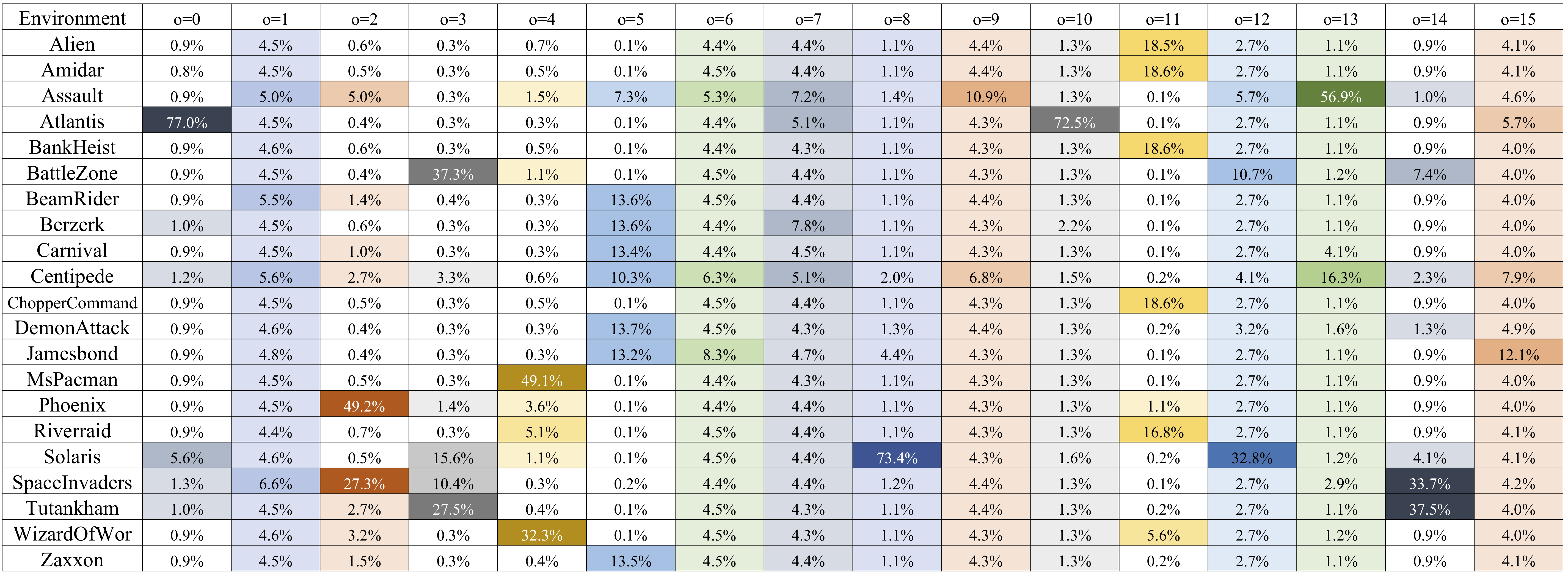
Figure 8: Option specialization across Atari games for a 16 option Option-Critic architecture trained in the many task learning setting.

B.5 Comparison with methods for multi-task and lifelong learning

In this work we explore a relatively straightforward application of multi-task learning on the Atari games. Following conventions in multi-task learning [3], as the action space is different with varying sizes across games, all parts of the network are shared with the exception of a task specific layer in the last layer of the policy over primitive actions. This a somewhat arbitrary choice of the extent of weight sharing in light of recent work that focuses on more dynamic sharing patterns in multi-task learning, lifelong learning, and continual learning settings [29, 23, 32, 34, 6, 33, 10, 17, 30, 31]. A more dynamic weight sharing pattern should allow the hierarchical option-critic architecture to potentially achieve better sample efficiency in a multi-task learning setting. However, we leave analysis of the proper way to achieve this in a general sense to future work as it is largely orthogonal to our main contribution of presenting policy gradient theorems to optimize a deep hierarchy of options.

Our approach is also orthogonal to recent approaches improving the efficiency of multi-task learning through a learned curriculum learning process [36, 8]. In the setting we explore, all models train on the games in a balanced fashion throughout time and the agent is not assumed to have any control over which environment it trains on. Controlling the curriculum of games to train on could also potentially improve the efficacy of our approach.

References

• Bacon et al. [2017] Pierre-Luc Bacon, Jean Harb, and Doina Precup. The option-critic architecture. 2017.
• Bellemare et al. [2013] M. G. Bellemare, Y. Naddaf, J. Veness, and M. Bowling. The arcade learning environment: An evaluation platform for general agents. Journal of Artificial Intelligence Research, 47:253–279, jun 2013.
• Caruana [1997] Rich Caruana. Multitask learning. Machine Learning, 28(1):41–75, 1997. doi: 10.1023/A:1007379606734. URL http://dx.doi.org/10.1023/A:1007379606734.
• Daniel et al. [2016] Christian Daniel, Herke Van Hoof, Jan Peters, and Gerhard Neumann. Probabilistic inference for determining options in reinforcement learning. Machine Learning, 104(2-3):337–357, 2016.
• Dayan and Hinton [1993] Peter Dayan and Geoffrey E Hinton. Feudal reinforcement learning. In Advances in neural information processing systems, pages 271–278, 1993.
• Fernando et al. [2017] Chrisantha Fernando, Dylan Banarse, Charles Blundell, Yori Zwols, David Ha, Andrei A Rusu, Alexander Pritzel, and Daan Wierstra. Pathnet: Evolution channels gradient descent in super neural networks. arXiv preprint arXiv:1701.08734, 2017.
• Fox et al. [2017] Roy Fox, Sanjay Krishnan, Ion Stoica, and Ken Goldberg. Multi-level discovery of deep options. arXiv preprint arXiv:1703.08294, 2017.
• Graves et al. [2018] Alex Graves, Marc G Bellemare, Jacob Menick, Remi Munos, and Koray Kavukcuoglu. Automated curriculum learning for neural networks. ICML, 2018.
• Harb et al. [2017] Jean Harb, Pierre-Luc Bacon, Martin Klissarov, and Doina Precup. When waiting is not an option: Learning options with a deliberation cost. arXiv preprint arXiv:1709.04571, 2017.
• Kirkpatrick et al. [2017] James Kirkpatrick, Razvan Pascanu, Neil Rabinowitz, Joel Veness, Guillaume Desjardins, Andrei A Rusu, Kieran Milan, John Quan, Tiago Ramalho, Agnieszka Grabska-Barwinska, et al. Overcoming catastrophic forgetting in neural networks. Proceedings of the National Academy of Sciences, page 201611835, 2017.
• Klissarov et al. [2017] Martin Klissarov, Pierre-Luc Bacon, Jean Harb, and Doina Precup. Learnings options end-to-end for continuous action tasks. arXiv preprint arXiv:1712.00004, 2017.
• Konda and Tsitsiklis [2000] Vijay R Konda and John N Tsitsiklis. Actor-critic algorithms. In Advances in neural information processing systems, pages 1008–1014, 2000.
• Konidaris et al. [2011] George Konidaris, Scott Kuindersma, Roderic A Grupen, and Andrew G Barto. Autonomous skill acquisition on a mobile manipulator. In AAAI, 2011.
• Kulkarni et al. [2016] Tejas D Kulkarni, Karthik Narasimhan, Ardavan Saeedi, and Josh Tenenbaum. Hierarchical deep reinforcement learning: Integrating temporal abstraction and intrinsic motivation. In Advances in neural information processing systems, pages 3675–3683, 2016.
• Levy et al. [2017] Andrew Levy, Robert Platt, and Kate Saenko. Hierarchical actor-critic. arXiv preprint arXiv:1712.00948, 2017.
• Levy and Shimkin [2011] Kfir Y Levy and Nahum Shimkin. Unified inter and intra options learning using policy gradient methods. In European Workshop on Reinforcement Learning, pages 153–164. Springer, 2011.
• Li and Hoiem [2016] Zhizhong Li and Derek Hoiem. Learning without forgetting. In European Conference on Computer Vision, pages 614–629. Springer, 2016.
• Machado et al. [2017] Marlos C Machado, Marc G Bellemare, Erik Talvitie, Joel Veness, Matthew Hausknecht, and Michael Bowling. Revisiting the arcade learning environment: Evaluation protocols and open problems for general agents. arXiv preprint arXiv:1709.06009, 2017.
• Mankowitz et al. [2016] Daniel J Mankowitz, Timothy A Mann, and Shie Mannor. Adaptive skills adaptive partitions (asap). In Advances in Neural Information Processing Systems, pages 1588–1596, 2016.
• Mann et al. [2015] Timothy A Mann, Shie Mannor, and Doina Precup. Approximate value iteration with temporally extended actions. Journal of Artificial Intelligence Research, 53:375–438, 2015.
• McGovern and Barto [2001] Amy McGovern and Andrew G Barto. Automatic discovery of subgoals in reinforcement learning using diverse density. In Proceedings of the Eighteenth International Conference on Machine Learning, pages 361–368. Morgan Kaufmann Publishers Inc., 2001.
• Menache et al. [2002] Ishai Menache, Shie Mannor, and Nahum Shimkin. Q-cut—dynamic discovery of sub-goals in reinforcement learning. In European Conference on Machine Learning, pages 295–306. Springer, 2002.
• Misra et al. [2016] Ishan Misra, Abhinav Shrivastava, Abhinav Gupta, and Martial Hebert. Cross-stitch networks for multi-task learning. In Proceedings of the IEEE Conference on Computer Vision and Pattern Recognition, pages 3994–4003, 2016.
• Mnih et al. [2015] V. Mnih, K. Kavukcuoglu, D. Silver, A. A. Rusu, J. Veness, M. G. Bellemare, A. Graves, M. Riedmiller, A. K. Fidjeland, G. Ostrovski, et al. Human-level control through deep reinforcement learning. Nature, 518(7540):529, 2015.
• Mnih et al. [2016] Volodymyr Mnih, Adria Puigdomenech Badia, Mehdi Mirza, Alex Graves, Timothy Lillicrap, Tim Harley, David Silver, and Koray Kavukcuoglu. Asynchronous methods for deep reinforcement learning. In International Conference on Machine Learning, pages 1928–1937, 2016.
• Niekum [2013] Scott D Niekum. Semantically grounded learning from unstructured demonstrations. University of Massachusetts Amherst, 2013.
• Precup [2000] Doina Precup. Temporal abstraction in reinforcement learning. University of Massachusetts Amherst, 2000.
• Puterman [1994] Martin L Puterman. Markov decision processes: Discrete dynamic stochastic programming, 92–93, 1994.
• Riemer et al. [2015] Matthew Riemer, Sophia Krasikov, and Harini Srinivasan. A deep learning and knowledge transfer based architecture for social media user characteristic determination. In Proceedings of the third International Workshop on Natural Language Processing for Social Media, pages 39–47, 2015.
• Riemer et al. [2016] Matthew Riemer, Elham Khabiri, and Richard Goodwin. Representation stability as a regularizer for improved text analytics transfer learning. arXiv preprint arXiv:1704.03617, 2016.
• Riemer et al. [2017] Matthew Riemer, Michele Franceschini, Djallel Bouneffouf, and Tim Klinger. Generative knowledge distillation for general purpose function compression. NIPS 2017 Workshop on Teaching Machines, Robots, and Humans, 5:30, 2017.
• Rosenbaum et al. [2018] Clemens Rosenbaum, Tim Klinger, and Matthew Riemer. Routing networks: Adaptive selection of non-linear functions for multi-task learning. ICLR, 2018.
• Rusu et al. [2015] Andrei A Rusu, Sergio Gomez Colmenarejo, Caglar Gulcehre, Guillaume Desjardins, James Kirkpatrick, Razvan Pascanu, Volodymyr Mnih, Koray Kavukcuoglu, and Raia Hadsell. Policy distillation. arXiv preprint arXiv:1511.06295, 2015.
• Rusu et al. [2016] Andrei A Rusu, Neil C Rabinowitz, Guillaume Desjardins, Hubert Soyer, James Kirkpatrick, Koray Kavukcuoglu, Razvan Pascanu, and Raia Hadsell. Progressive neural networks. arXiv preprint arXiv:1606.04671, 2016.
• Sahni et al. [2017] Himanshu Sahni, Saurabh Kumar, Farhan Tejani, and Charles Isbell. Learning to compose skills. arXiv preprint arXiv:1711.11289, 2017.
• Sharma et al. [2017] S. Sharma, A. Jha, P. Hegde, and B. Ravindran. Learning to multi-task by active sampling. arXiv preprint arXiv:1702.06053, 2017.
• Shu et al. [2017] Tianmin Shu, Caiming Xiong, and Richard Socher. Hierarchical and interpretable skill acquisition in multi-task reinforcement learning. arXiv preprint arXiv:1712.07294, 2017.
• Silver and Ciosek [2012] David Silver and Kamil Ciosek. Compositional planning using optimal option models. arXiv preprint arXiv:1206.6473, 2012.
• Şimşek and Barto [2009] Özgür Şimşek and Andrew G Barto. Skill characterization based on betweenness. In Advances in neural information processing systems, pages 1497–1504, 2009.
• Stolle and Precup [2002] Martin Stolle and Doina Precup. Learning options in reinforcement learning. In International Symposium on abstraction, reformulation, and approximation, pages 212–223. Springer, 2002.
• Sutton et al. [1999] Richard S Sutton, Doina Precup, and Satinder Singh. Between mdps and semi-mdps: A framework for temporal abstraction in reinforcement learning. Artificial intelligence, 112(1-2):181–211, 1999.
• Sutton et al. [2000] Richard S Sutton, David A McAllester, Satinder P Singh, and Yishay Mansour. Policy gradient methods for reinforcement learning with function approximation. In Advances in neural information processing systems, pages 1057–1063, 2000.
• Vezhnevets et al. [2016] Alexander Vezhnevets, Volodymyr Mnih, Simon Osindero, Alex Graves, Oriol Vinyals, John Agapiou, et al. Strategic attentive writer for learning macro-actions. In Advances in neural information processing systems, pages 3486–3494, 2016.
• Vezhnevets et al. [2017] Alexander Sasha Vezhnevets, Simon Osindero, Tom Schaul, Nicolas Heess, Max Jaderberg, David Silver, and Koray Kavukcuoglu. Feudal networks for hierarchical reinforcement learning. arXiv preprint arXiv:1703.01161, 2017.