The -parity Violating Decays of
Charginos and Neutralinos
in the B-L MSSM
Abstract
The MSSM is the MSSM with three right-handed neutrino chiral multiplets and gauged symmetry. The symmetry is broken by the third family right-handed sneutrino acquiring a VEV, thus spontaneously breaking -parity. Within a natural range of soft supersymmetry breaking parameters, it is shown that a large and uncorrelated number of initial values satisfy all present phenomenological constraints; including the correct masses for the , bosons, having all sparticles exceeding their present lower bounds and giving the experimentally measured value for the Higgs boson. For this “valid” set of initial values, there are a number of different LSPs, each occurring a calculable number of times. We plot this statistically and determine that among the most prevalent LSPs are chargino and neutralino mass eigenstates. In this paper, the -parity violating decay channels of charginos and neutralinos to standard model particles are determined, and the interaction vertices and decay rates computed analytically. These results are valid for any chargino and neutralino, regardless of whether or not they are the LSP. For chargino and neutralino LSPs, we will– in a subsequent series of papers –present a numerical study of their RPV decays evaluated statistically over the range of associated valid initial points.
1 Introduction
The discovery of the Higgs particle at the Large Hadron Collider (LHC) Aad:2012tfa ; Chatrchyan:2012xdj completed the experimental search for the spectrum of the “standard model” of particle physics. The three chiral families of quarks and leptons, as well as the gluons, the , and photon vector bosons corresponding to the standard model gauge group , had long since been known. However, the discovery of the Higgs scalar boson had special significance, since its vacuum expectation value (VEV) is required to spontaneously break the electroweak symmetry to the of electromagnetism and to give masses to the matter fields and the electroweak vector bosons. This completion of the standard model confirms that the “low energy” world we observe is made up of precisely this spectrum, the particles of which interact with each other via strong, weak and electromagnetic gauge interactions.
However, as it presently stands, the standard model has several very significant shortcomings. To begin with, there is no theoretical explanation for either the particle content or the explicit gauge group of the interactions. Furthermore, the standard model contains a large number of undetermined parameters. These include 1) the Yukawa couplings that give rise, after spontaneous electroweak breaking, to the masses of the quarks/leptons, 2) the gauge coupling parameters of the strong, weak and electromagnetic interactions as well as 3) the mass and coupling parameters of the pure Higgs boson Lagrangian. At the present state of our knowledge, these parameters are simply input at a fixed scale so as to lead to the experimentally determined values of the particle masses and the observed strength of the gauge interactions. Finally, the standard model makes no attempt to couple its spectrum to gravitation, let alone to explain the origin of this fundamental force. It seems clear, therefore, that despite the remarkable successes of the standard model, there must exist “beyond the standard model” physics which addresses and solves all of the shortcomings discussed above.
At the present time, the only fundamental theory that would appear to have the potential to do this is superstring/M-theory–although at the price of introducing spontaneously broken supersymmetry (SUSY) as a major component of “beyond the standard model” physics. In this paper, we will consider a specific subset of such theories; namely, the heterotic string Gross:1984dd and its possible origin as a vacuum state of M-theory, called heterotic M-theory Horava:1996ma ; Lukas:1997fg ; Lukas:1998ew ; Lukas:1998yy ; Lukas:1998tt . We do this for several important reasons. First of all, it is known using a series of papers Evans:1985vb ; Donagi:2000fw ; Donagi:2004ia ; Braun:2005zv that heterotic M-theory, when compactified on a specific Calabi-Yau threefold Braun:2005nv , exhibits an observable sector with exactly the quark/lepton and Higgs spectrum of the so-called Minimal Supersymmetric Standard Model (MSSM); that is, three families of quark and lepton chiral superfields, each family with a right-handed neutrino chiral multiplet, and two doublets of Higgs chiral supermultiplets. Furthermore, the observable sector of this heterotic M-theory vacuum “contains” the gauge group ; significantly, multiplied by an additional gauged Abelian group , where and are baryon number and lepton number respectively. Below the scale of both spontaneous and SUSY breaking, the observable sector of this theory contains precisely the particle spectrum and gauge group of the standard model. It has also been demonstrated that the potential energy functions of the geometric, vector bundle and five-brane moduli can, in principle, be calculated and the vacuum for these moduli stabilized; see, for example Anderson:2011cza ; Buchbinder:2002pr ; Donagi:1999jp ; Lima:2001jc .
Secondly, it has been shown in a number of contexts Anderson:2009nt ; Anderson:2009ge ; Blesneag:2015pvz ; Blesneag:2016yag that the Yukawa couplings are, in principle, directly computable as integrals over the products of the harmonic representatives of the associated sheaf cohomology classes Braun:2006me . Similarly, gauge couplings are potentially calculable from the threshold corrections at the string unification scale Deen:2016vyh ; Kaplunovsky:1992vs ; Kaplunovsky:1995jw ; Mayr:1993kn ; Dienes:1995sq ; Dienes:1996du ; Nilles:1997vk ; Ghilencea:2001qq ; deAlwis:2012bm ; Bailin:2014nna . Finally, making SUSY a local symmetry produces gravitation as the associated gauge field, although in the form of a gravity supermultiplet containing the gravitino as well as the graviton. That is, the existence of supersymmetry puts gravity on par with the strong, weak and electromagnetic gauge interactions. This property enables fundamental theories of early universe cosmology to occur; both within the context of inflation Deen:2016zfr ; Ferrara:2015cwa ; Linde:2016bcz or “bouncing universe” Koehn:2012ar ; Battarra:2014tga scenarios. For all of these reasons, the heterotic string and its possible origin as a vacuum state of heterotic M-theory appears to be a strong candidate for the theory of “beyond the standard model” physics.
With this in mind, we will confine ourselves in this paper to “beyond the standard model” physics arising in the observable sector of the heterotic M-theory vacuum discussed above. At energies below the Calabi-Yau scale, the observable sector is precisely the MSSM with three right-handed neutrino chiral multiplets and gauge group . Because of the existence of the additional gauge factor, we call this theory the MSSM. The additional gauged symmetry plays a fundamental role in our analysis. Recall that to prevent unacceptably rapid nucleon decay in the conventional MSSM, it is necessary to postulate the existence of a finite symmetry group called -parity. This acts on component fields as , where is the associated spin. While this finite symmetry indeed accomplishes its purpose, -parity is, from a theoretical viewpoint, completely ad hoc–without any fundamental justification. However, continuous symmetry arises naturally as a consequence of the compactification of heterotic M-theory and, indeed, has long been known in a non-supersymmetric context to be the minimal extra gauging of the standard model that remains quantum mechanically anomaly free. That is, the gauged that arises in our context gives a “natural way” to suppress unwanted baryon and lepton number violating decays. Of course, the symmetry must be spontaneously broken at a scale sufficiently high to account for the fact that its associated massive vector boson has, so far, not been observed. As discussed in the text, symmetry is spontaneously broken by the right-handed sneutrino acquiring an non-vanishing VEV. This breaks lepton number and, hence, symmetry. However, baryon number remains unbroken and, therefore, proton decay continues to be suppressed below its present experimental bounds. However, the parameters of the MSSM must be chosen so as to adequately suppress lepton number violating processes. This will indeed be the case, as originally discussed in Marshall:2014cwa and elaborated on in the text below.
We conclude that the MSSM is the simplest possible phenomenologically realistic low energy theory of heterotic superstring/M-theory; being the exact MSSM with right-handed neutrinos and spontaneously broken -parity This theory was originally presented in the series of papers Braun:2005nv ; Ambroso:2009jd ; Ambroso:2009sc ; Ambroso:2010pe ; Ovrut:2012wg ; Ovrut:2014rba ; Ovrut:2015uea . It is interesting to point out that the MSSM was also constructed from a “bottom-up” point of view, completely unrelated to superstring theory FileviezPerez:2008sx ; Barger:2008wn ; FP:2009gr ; Everett:2009vy ; FileviezPerez:2012mj ; Perez:2013kla . This simply postulated that the standard model should be extended to supersymmetry with three right-handed neutrino chiral multiplets–that is, the MSSM–with the problem of motivating -parity solved by postulating spontaneously broken gauged symmetry. That is, the MSSM as the simplest “beyond the standard model” theory is obtained from both a “top-down” superstring analysis as well as a “bottom-up” phenomenological approach. It follows that the MSSM represents a strongly motivated “beyond the standard model” paradigm. Decay channels and decay rates for various sparticles of arbitrary mass have been identified and computed within the context of the -parity conserving MSSM. Some of these have been searched for experimentally; so far without success. In the MSSM, these same decay channels remain. In addition, there are new -parity violating (RPV) decay modes that now occur. These are, however, generically much weaker and, hence, harder to search for experimentally. There is, however, an important exception to this!
As is well-known, see for example Martin:1997ns , the original -parity invariant MSSM must contain a lightest supersymmetric particle (LSP) that is completely stable and cannot further decay to standard model particles. The mass of this LSP depends on the scale of spontaneous SUSY breaking introduced into the model. For different choices of input parameters, the LSP sparticle will vary but, in all cases, is stable and cannot further decay. However, this fundamentally changes in the MSSM. In the MSSM, prior to the spontaneous breaking of , there will, as in the MSSM, be an LSP whose species again depends on the input initial conditions. As in the MSSM, this LSP cannot decay via -parity preserving processes. However, the spontaneous breaking of in this theory now leads to specific, and completely calculable, -parity violating decays of this LSP into standard model particles. Not only are the decay modes of the LSP explicitly determined, but the associated vertex coefficients and, hence, the decay rates and branching ratios are exactly calculable. It follows that these -parity violating decays should be amenable to direct detection at the ATLAS and CMS detectors at the LHC. Detection of these processes would not only be an explicit indication of “beyond the standard model” physics, but would also strongly hint at the existence of SUSY with spontaneously broken -parity.
The first calculation of such an -parity decay was presented in Marshall:2014cwa ; Marshall:2014kea . In this example, the initial conditions of the MSSM were chosen so that the LSP was the lightest real scalar superpartner of the top quark; the so-called admixture stop. Its -parity violating decay modes and branching ratios were determined theoretically. We refer the reader to Marshall:2014cwa ; Marshall:2014kea for details. In recent work, an ATLAS group analyzed the relevant LHC data looking for these experimental signatures Aaboud:2017opj . None were found, but a new experimental lower bound on the stop mass was determined. We emphasize that the lightest stop LSP was chosen as a “test case” since it is exotic, carrying both color and electric charge, and also has a large production cross section. Therefore, the stop could never have been chosen as the LSP in the ordinary MSSM, since it would be stable and contribute to at least a portion of dark matter, which must be neutral in all interactions. As shown in Ovrut:2014rba ; Ovrut:2015uea however, the stop sparticle occurs as the LSP for only a relatively small fraction of possible initial conditions in the MSSM. As discussed in Ovrut:2014rba ; Ovrut:2015uea , and analyzed in more detail in this paper, almost all other sparticles are much more likely to be the LSP in the MSSM. In particular, due both to their frequent appearance as the LSP and because their experimental signatures are easily detected by the LHC experimental groups, the -parity violating decays of both charginos and neutralinos are very interesting to analyze. Therefore, in this paper, we determine the -parity violating decay modes for both charginos and neutralinos, compute the explicit interaction coefficients for each such mode and calculate the explicit decay rates. We emphasize that the results of this paper are applicable to RPV decays of any chargino or neutralino. However, they are most easily experimentally observed when applied to the LSP of the MSSM. Specifically, we do the following.
In Section 2, we give a brief summary of the MSSM. In particular, the spontaneous breaking of gauged symmetry by a non-vanishing VEV of the third family right-handed sneutrino is discussed. The associated -parity violating interactions induced in the Lagrangian are presented in detail. The VEV of the right-handed sneutrino produces a mixing of the third family right-hand neutrino and the three left-handed neutrinos with all fermionic superpartners of the neutral gauge bosons and the up and down neutral Higgsinos. This is presented in Section 3. The general form of this mass matrix is given, as well as the explicit form of the unitary matrix required to diagonalize it. However, in that section, we focus on the diagonal left-handed neutrino Majorana submatix only. The mass eigenvalues of this matrix can be determined from the explicit form of the PMNS mixing matrix as well as the off-diagonal left-handed neutrino matrix . This latter matrix is a function of the -parity violating parameters as well as three additional quantities. The result is compared with the experimentally determined mass eigenvalues of both the “normal” and the “inverted” neutrino mass hierarchies. In Section 4, we list all of the presently known experimental data that must be satisfied in any phenomenologically acceptable vacuum. These include the masses of the , electroweak vector bosons, the Higgs mass, the present lower bounds on the SUSY sparticles and so on. Having done this, we present the mass interval in which we will statistically throw all dimensionful parameters of the soft SUSY breaking terms. The reason for choosing the specific median value and width of this interval is discussed in detail. Having presented this interval, we do a statistical analysis involving 100 million independent throws. A plot of the the “valid” points, that is, all parameters solving all required phenomenological bounds, is given and analyzed. A histogram of the LSPs associated with these valid points is presented. Section 5 is devoted to analyzing the mass matrices, including the terms induced by both spontaneous electroweak and -parity violation, for both the charginos and, independently, for the neutralinos of the MSSM. Important technical details of these calculations are discussed in the Appendix. The mass eigenvalues and eigenstates are explicitly calculated for both charginos and neutralinos. In Section 6 we present the relevant portions of the complete MSSM Lagrangian, including the effect of both electroweak symmetry breaking and -parity violation. Rewriting the original fields in terms of the chargino and neutralino mass eigenstates calculated in the previous section, we determine the three-point interaction vertices involving either a chargino or a neutralino eigenstate decaying into two standard model particles. The Feynman diagrams associated with these decays are presented pictorially and, for each decay process, the exact expression for the vertex coefficient is given. Finally, in Section 7 we summarize the possible -parity violating decays with their associated vertex parameters. These are then used to compute the decay rate for each of these processes. We emphasize that the results we present are valid for any chargino and neutralino, regardless of whether or not they are the LSP.
Before continuing to our analysis of the -parity violating MSSM chargino and neutralino LSP decays, it is useful to point out that the subject of RPV in the MSSM and related supersymmetric particle physics models has a long history in the literature. Papers in this context, up to and including most of 2005, are cited and discussed in the comprehensive review in Barbier:2004ez . Relevant to the content of our present paper, this review discussed both explicit and, more briefly, spontaneous RPV due to both left- and right-chiral sneutrinos developing VEVs, the associated massless “Majoron”, and possibly gauging lepton number global symmetry to make the Majoron heavy. The review also discussed the RGEs in some RPV theories, the RPV decays of some of the LSPs in various models and their impact on theories of dark matter. More recently, the subject was reviewed in 2015 Mohapatra:2015fua . This discussed explicit RPV in the MSSM but, in particular, focussed on spontaneous breaking of -parity in theories where the standard model symmetry is extended by a gauged . This review post-dates the papers in Braun:2005nv ; Ambroso:2009jd ; Ambroso:2009sc ; Ambroso:2010pe ; Ovrut:2012wg ; Ovrut:2014rba ; Ovrut:2015uea and FileviezPerez:2008sx ; Barger:2008wn ; FP:2009gr ; Everett:2009vy ; FileviezPerez:2012mj ; Perez:2013kla and cites some of them. In particular, this review highlights what it refers to as “Minimal models with automatic -parity breaking”; that is, the MSSM. It then introduces, and devotes the remainder of the work, to models with two pairs of Higgs doublets. More recently, there was a comprehensive paper Dercks:2017lfq on these subjects within the context of the RPV-CMSSM; that is, the MSSM with an additional RPV trilinear coupling at the unification scale. Within this context, that paper discussed the RGEs, taking into account the then recently discovered Higgs mass, and the associated LSPs. It goes on to discuss the RPV decay of some of the LSPs; specifically the Bino neutralino and the stau sparticle. It is not the intention of our paper to review this vast RPV literature. We refer the readers to the references in the mentioned papers. We do wish to point out that, although some of the broad topics that occur in our present paper are mentioned and discussed in previous RPV literature, such as RG evolution, the associated LSP calculations and their RPV decays, relationship to neutrino masses and so on, these previous discussions all occur in contexts considerably different than the heterotic M-theory MSSM. The present paper works strictly within this context and presents specific results for both chargino and neutralino decays not previously discussed. Finally, we note that there has been significant experimental studies of chargino and neutralino decays in -parity conserving theories–see M. Tanabashi et al. (Particle Data Group), Phys. Rev. D 98, 030001 (2018). The main purpose of the present paper is to analyze RPV chargino and neutralino decays in the spontaneously broken RPV MSSM. Some of the present authors have already applied this formalism to RPV decays of admixture stop LSPs in Marshall:2014cwa ; Marshall:2014kea and to Wino chargino and Wino neutralino decays in Dumitru:2018nct –analyzing potential LHC signatures. Other LSP RPV decays, and the predictions for LHC signatures in this context, will be presented in future publications.
2 The B-L MSSM
In this section, we briefly review the contents of the MSSM theory relevant to a phenomenological discussion of its -parity violating decay processes and their potential signatures at the LHC.
The low energy manifestation of the “heterotic standard model”, that is, the MSSM, arises from the breaking of an GUT theory via two independent Wilson lines, denoted by and , associated with the diagonal generator of and the generator of respectively. These specific generators are chosen since it can be shown that there is no kinetic mixing of their respective Abelian gauge kinetic terms at any energy scale– thus simplifying the RG calculations Ovrut:2012wg . However, identical physical results will be obtained for any linear combination of these generators. Associated with these Wilson lines are two mass scales, and , with three possible relations between them; 1) , 2) and 3) . As discussed in Ovrut:2012wg , the masses in the first two relations can be adjusted so as to enforce exact unification at one loop of all gauge couplings at the SO(10) unification scale , whereas gauge unification cannot occur for the third mass relationship without accounting for threshold effects at the unification scale or the SUSY scale Deen:2016vyh ; Ovrut:2012wg ; Fundira:2017vip . For this reason, we will not consider the third option in this paper. The gauge coupling RG equations associated with each of the first two mass relations were discussed in detail in Ovrut:2012wg and, as far as low energy LHC phenomenology is concerned, give almost identical results. For specificity, therefore, in this paper we will focus on the first relationship and, without loss of accuracy, choose . The lower scale , which we henceforth denote by , is adjusted so as to obtain exact gauge coupling unification. We emphasize, however, that the low energy results predicted for the LHC are almost unchanged even if is chosen to yield only “approximate” gauge unification — with moderate sized gauge “thresholds”. Conventionally, the scale of supersymmetry breaking is defined to be
| (2.1) |
where and are the lightest and heaviest stop masses respectively; see ,for example, Ovrut:2015uea . Suffice it here to say that for supersymmetry breaking to occur between the electroweak scale and 10 TeV, which will be the case in this paper, the unification scale is found to be . Over the same range of supersymmetry breaking, however, the intermediate scale changes from to respectively Deen:2016vyh .
The details of the symmetry breaking and the respective mass spectra for this choice of Wilson line hierarchy were given in Ovrut:2012wg . Here, we simply note that in the mass regime between and , the gauge group is broken from to with the spectrum shown in Figure 1. This theory is referred to as the “left-right” model Senjanovic:1975rk ; Grimus:1993fx . As discussed above, for the supersymmetry breaking scales of interest in this paper, this mass regime will on average be considerably smaller than one order of magnitude in GeV.
At the “intermediate” scale , the second Wilson line breaks this “left-right” model down to the exact MSSM. This theory has the gauge group of the standard model augmented by an additional Abelian symmetry. As mentioned above, it is convenient– and equivalent –to use the Abelian group with the generator
| (2.2) |
in the RGE’s since the associated gauge kinetic term cannot mix with the gauge kinetic energy of . That is, the MSSM gauge group is chosen, for computational convenience, to be
| (2.3) |
The associated gauge couplings will be denoted by , , and . The spectrum, as shown in Figure 1, is exactly that of the MSSM with three right-handed neutrino chiral multiplets, one per family; that is, three generations of matter superfields
| (2.8) | |||||
| (2.13) |
along with two Higgs supermultiplets
| (2.14) |
The superpotential of the MSSM is given by
| (2.15) |
where flavor and gauge indices have been suppressed and the Yukawa couplings are three-by-three matrices in flavor space. In principle, the Yukawa matrices are arbitrary complex matrices. However, the observed smallness of the three CKM mixing angles and the CP-violating phase dictate that the quark Yukawa matrices be taken to be nearly diagonal and real. The charged lepton Yukawa coupling matrix can also be chosen to be diagonal and real. This is accomplished by moving the rotation angles and phases into the neutrino Yukawa couplings which, henceforth, must be complex matrices. Furthermore, the smallness of the first and second family fermion masses implies that all components of the up, down quark and charged lepton Yukawa couplings– with the exception of the (3,3) components –can be neglected for the purposes of the RG running. Similarly, the very light neutrino masses imply that the neutrino Yukawa couplings are sufficiently small so as to be neglected for the purposes of RG running. However, the , neutrino Yukawa couplings cannot be neglected for the calculations of the neutralino, neutrino and chargino mass matrices, as well as in decay rates/branching ratios. The -parameter can be chosen to be real, but not necessarily positive, without loss of generality. We implement these constraints in the remainder of our analysis.
Spontaneous supersymmetry breaking is assumed to occur in a hidden sector– a natural feature of both strongly and weakly coupled heterotic string theory –and be transmitted through gravitational mediation to the observable sector and, hence, to the MSSM. Since the MSSM first manifests itself at the scale , we will begin our analysis by presenting the most general soft supersymmetry breaking interactions at that scale. That is, at scale , the soft supersymmetry breaking Lagrangian is given by
| (2.16) | ||||
The parameter can be chosen to be real and positive without loss of generality. The gaugino soft masses can, in principle, be complex. This, however, could lead to CP-violating effects that are not observed. Therefore, we proceed by assuming they all are real. The -parameters and scalar soft mass can, in general, be Hermitian matrices in family space. Again, however, this could lead to unobserved flavor and CP violation. Therefore, we will assume they all are diagonal and real. Furthermore, we assume that only the (3,3) components of the up, down quark and charged lepton -parameters are significant and that the neutrino parameters are negligible for the RG running and all other purposes. For more explanation of these assumptions, see Ovrut:2015uea .
As discussed in Ovrut:2015uea , without loss of generality one can assume that the third generation right-handed sneutrino, since it carries the appropriate and charges, spontaneous breaks the symmetry by developing a non-vanishing VEV
| (2.17) |
This VEV spontaneously breaks down to the hypercharge gauge group . We denote the associated gauge parameter by . However, since sneutrinos are singlets under the gauge group, it does not break any of the SM symmetries. At a lower mass scale, electroweak symmetry is spontaneously broken by the neutral components of both the up and down Higgs multiplets acquiring non-zero VEV’s. In combination with the right-handed sneutrino VEV, this also induces a VEV in each of the three generations of left-handed sneutrinos. The notation for the relevant VEVs is
| (2.18) |
where is the generation index. The neutral gauge boson that becomes massive due to symmetry breaking, , has a mass at leading order, in the relevant limit that , of
| (2.19) |
where
| (2.20) |
The second term in the parenthesis is a small effect due to mixing in the neutral gauge boson sector.
A discussion of the neutrino masses is presented in the next section, where they are shown to be roughly proportional to the and parameters. It follows that and . In this phenomenologically relevant limit, the minimization conditions of the potential are simple, leading to the VEV’s
| (2.21) | ||||
| (2.22) | ||||
| (2.23) | ||||
| (2.24) |
where
| (2.25) |
Here, the first two equations correspond to the sneutrino VEVs. The third and fourth equations are of the same form as in the MSSM, but new scale contributions to and shift their values significantly compared to the MSSM. Eq. (2.21) can be used to re-express the mass as
| (2.26) |
This makes it clear that, to leading order, the mass is determined by the soft SUSY breaking mass of the third family right-handed sneutrino. The term proportional to is insignificant in comparison and, henceforth, neglected in our calculations.
Recall that -parity is defined as
| (2.27) |
It follows that a direct consequence of generating a VEV for the third family sneutrino is the spontaneous breaking of symmetry and, hence, -parity. The -parity violating operators induced in the superpotential are given by
| (2.28) |
where
| (2.29) |
and is the th component of the diagonal lepton Yukawa coupling. This general pattern of -parity violation is referred to as bilinear -parity breaking and has been discussed in many different contexts Mukhopadhyaya:1998xj ; Chun:1998ub ; Chun:1999bq ; Hirsch:2000ef . In addition, the Lagrangian contains bilinear terms generated by and in the super-covariant derivatives. These are
| (2.30) | ||||
The consequences of spontaneous -parity violation are quite interesting, and have been discussed in a number of papers FileviezPerez:2008sx ; Barger:2008wn ; FP:2009gr ; Everett:2009vy ; FileviezPerez:2012mj ; Perez:2013kla ; Ghosh:2010hy ; Barger:2010iv ; Mohapatra:1986aw . In this paper, we will present the decay channels for arbitrary mass charginos and neutralinos, and analytically determine their decay rates. However, in a series of following works, we will explore the phenomenological consequences of the -parity violating (RPV) decays of the lightest, and next-to-lightest, supersymmetric particles; referred to as the LSP and NLSP respectively. These decays are potentially observable at the ATLAS detector of the LHC. Hence, if detected, these explicit decays could verify the existence of low energy supersymmetry, shed light on the structure of the precise supersymmetric model– such as the MSSM –and, as will become apparent, even constrain whether the neutrino mass hierarchy is “normal” or “inverted”. However, as is clear from expressions (2.28) and (2.30), these results will depend explicitly on the values of the parameters , and , defined in (2.29) and (2.22) respectively. In turn, these parameters are dependent on the present experimental values of the neutrino masses. These reduce the number of independent RPV parameters from six to one and potentially restrict the value of the remaining independent coefficient. For that reason, we will discuss the neutrino masses and their direct relationship to the and parameters in the next section.
3 Neutrino Masses and the RPV Parameters
As discussed in Marshall:2014cwa ; Marshall:2014kea ; Ovrut:2014rba ; Ovrut:2015uea ; Barger:2010iv , it follows from the above Lagrangian that the third family right-handed neutrino and the three left-chiral neutrinos , mix with the fermionic superpartners of the neutral gauge bosons and with the up- and down- neutral Higgsinos. In other words, the neutralinos now mix with the neutral fermions of the standard model. The mixing with the third-family right-handed sneutrino, through terms proportional to and , allows the third-family right-handed sneutrino to act as a seesaw field giving rise to Majorana neutrino masses. This is reviewed in this section.
First, we note that this paper is focused on the consequences of RPV decays at the LHC. There is the possibility that the RPV parameters are so small that the LSP decay length is too long for it to decay within the detector. Then the LSP would be effectively stable within the detector. For certain cases, such effectively stable sparticles have been searched for in ATLAS:2014fka . If the LSP decay length is small enough to decay within the detector, but greater than about 1 mm, this would lead to “displaced” vertices, such as those searched for in, for example, Aad:2015rba . In the present paper, we will choose parameters so that the decay length of the LSP, whatever sparticle that may be, is less than about 1 mm. We refer to such decays as “prompt” decays. Therefore, even though the analysis in this work is valid for any mass chargino and neutralino, should we choose the initial conditions so that they are the LSP, then their RPV decays will be prompt.
As was shown in the case of stops and sbottoms in Marshall:2014cwa ; Marshall:2014kea , prompt decays require the RPV parameters to be large enough to allow for significant Majorana neutrino masses. We expect the same to hold true for a variety of LSPs. Therefore, in this paper we focus on the case of significant Majorana neutrino masses. Note that, in addition to these Majorana neutrino masses, there can be pure Dirac mass contributions coming from the neutrino Yukawa coupling. The components , which couple the left-handed neutrinos to the third-family right-handed neutrino, allow the third-family right-handed neutrino to act as a seesaw field and give rise to Majorana neutrino masses. The other components, and , couple the left-handed neutrinos to the first- and second-family right-handed neutrinos. Note that in this model, the heavy third-family right-handed neutrino acts as a seesaw field, while the first- and second-family right-handed neutrinos remain as light sterile neutrinos. This means that the Dirac mass terms related to and can give rise to active-sterile oscillations in the neutrino sector. There have been some experimental hints of such oscillations, see PDG for review. However, it is not yet clear that these results are due to true active-sterile oscillations. Hence, we proceed under the assumption that no such oscillations exist and that the and components of the neutrino Yukawa coupling must, therefore, be negligible, so they do not appear in the neutralino mass matrix below. It may be interesting to revisit the question of active-sterile neutrino oscillations in the MSSM in the future, perhaps after there is more experimental data.
In the basis with , the neutralino mass matrix is of the form
| (3.1) |
where is a six-by-six matrix of order a TeV given by
| (3.2) |
and is a six-by-three matrix
| (3.3) |
of order an MeV. This allows the mass matrix to be diagonalized perturbatively. Note that we have suppressed all terms of the form in since both and the neutrino Yukawa parameters are small. In addition, we emphasize that since only the third family right-handed sneutrino gets a non-vanishing VEV, only couples to the gauginos/Higgsinos. It follows that only the Dirac mass of the third-family neutrino enters the above mass matrix, whereas the the first and second family Dirac neutrino masses are excluded.
The entire mass matrix in (3.1) can be diagonalized to
| (3.4) |
with
| (3.5) |
where is the matrix that diagonalizes given in eq. (3.2). Requiring that be diagonal yields
| (3.6) |
The second matrix on the right-hand side of rotates away the neutralino/left-handed neutrino mixing, whereas the first matrix diagonalizes the six neutralino/third family right-handed neutrino states as well as the three left-chiral neutrino states. In this section, we will consider the diagonal left-handed neutrino Majorana mass matrix only, returning to the diagonal neutralino mass matrix later in the paper.
The diagonal left-chiral neutrino Majorana mass matrix is found to be
| (3.7) | ||||
The matrix is given by Marshall:2014cwa
| (3.8) |
where
| (3.9) | ||||
| (3.10) | ||||
| (3.11) | ||||
and
| (3.12) |
As will be discussed in detail below, the soft mass parameters are all initialized statistically at the scale , whereas the measured values of the gauge couplings are introduced at the electroweak scale. All of these parameters are then run to the appropriate energy scale using the RGEs discussed in detail in Ovrut:2015uea . Additionally, the value of tan will be chosen statistically within a physically relevant interval and, for a given value of tan, the parameters and are the measured Higgs VEVs. Finally, for any given set of statistical initial data, we fine-tune the value of the parameter using equation (2.23), so as to obtain the experimental value of the electroweak gauge boson and, hence, the measured values for as well. The Pontecorvo-Maki-Nakagawa-Sakata matrix is
| (3.13) | |||||
with . The mixing angles and phases are determined by neutrino experiments. For the mixing angles, we use the values and uncertainties from Capozzi:2018ubv . They are
| (3.14) |
for both the normal and inverted neutrino mass hierarchies. For , however, the best-fit values depend on the hierarchy, and the data admits multiple best-fit values. In the normal hierarchy, one finds
| (3.15) |
while in the inverted hierarchy
| (3.16) |
In this paper, we will do a complete study of all four of the cases in equations (3.15) and (3.16). Regarding the CP-violating phase, , we use the recent results in Capozzi:2018ubv that in the normal hierarchy
| (3.17) |
while in the inverted hierarchy
| (3.18) |
In addition, note that there is only one “Majorana” phase, that is, parameter , since in both the normal and the inverted hierarchy one of the neutrinos is massless and, therefore, does not have a Majorana mass. The value of is unknown and, hence, in this paper we will simply throw it statistically in the interval .
The mathematical expressions for the mass eigenvalues of the Majorana neutrino mass matrix can be constructed from the A,B,C components of given in (3.9), (3.10) and (3.11) respectively, as well as from the PMNS matrix given in (3.13). This has been done in detail in Marshall:2014cwa , to which we refer the reader for details. Given values for all the relevant parameters discussed above, and the measured values for the neutrino mass eigenvalues for the normal and inverted hierarchies, this allows one to solve for the RPV parameters , . Respectively, the experimental values of the mass eigenvalues of the normal and inverted hierarchies are PDG
-
•
Normal Hierarchy:
(3.19) -
•
Inverted Hierarchy:
(3.20)
In each case, all three parameters as well as two of the parameters can be determined in terms of a third parameter. The explicit expressions, of course, differ in the normal and inverted hierarchy cases, and are presented in detail in Marshall:2014cwa . These are encoded into the computer program by which we determine all decay rates and branching ratios and won’t be presented here. Suffice it to say that, in each case, which parameter is inputted is undetermined. Thus, we will statistically decide which of the three dimension one parameters is selected. Furthermore, we choose its value by randomly throwing it to be in the interval GeV with a log-uniform distribution. We limit the upper bound to GeV to avoid excessive fine-tuning in the neutrino masses. Furthermore, we cut off the lower bound at GeV– although this could be taken to –to enhance the readability of our branching ratio plots. It is important to note that, having statistically chosen one of the parameters in the above range, the other two parameters are determined by the computer code and are not necessarily bounded by this interval. For example, at least one of the remaining two parameters could, in principle, be considerably larger than GeV. If so, this could have important consequences for for the suppression of lepton number violating interactions. The reason is the following.
It was shown in Barbier:2004ez , and discussed in Marshall:2014cwa , that the experimental bound on the decay of leads to the constraint on and that
| (3.21) |
Scanning the initial parameters in the MSSM, using (2.19), (2.26) and the values for the gauge parameters discussed in Ovrut:2012wg , we find that this becomes
| (3.22) |
Therefore, to adequately suppress lepton number violating decays, it is essential to show that this bound is satisfied for any physically interesting set of initial data in this analysis. At the end of Section 4, we will demonstrate that for the LSPs of interest in this and in the follow-up papers, that is, for charginos and neutralinos, constraint (3.22) is easily satisfied.
4 Physically Acceptable Vacua
Having stated the structure of the MSSM, and defined all of the associated parameters, we now use the computer code specified in detail in Ovrut:2015uea to find the initial values of the parameters leading to completely acceptable physical vacua. The choice of initial parameters will be subject to all the constraints listed previously in Sections 2 and 3. For example, as discussed in Section 2, we will assume that the ratio of the Wilson line masses and is such that all gauge parameters unify at , that all quark and charged lepton Yukawa couplings can be taken to be nearly diagonal and real and, as discussed in Section 3, only the components of the neutrino Yukawa couplings are non-negligible. In addition, we solve for the physically acceptable initial conditions subject to several new, and important, constraints. These are the following:
-
•
Scattering Range of the Dimensionful Soft SUSY Breaking Parameters:
(4.1)
The median supersymmetry breaking mass and the parameter are chosen so that the range of dimensionful soft masses can have random values from just above the electroweak scale to a scale approaching the upper bound of what will be observable at the LHC. That is, range (4.1) is approximately GeV TeV.
-
•
Random Sign of the Soft SUSY Breaking Parameters , and :
(4.2)
The sign of and the various soft parameters of the form and are chosen randomly to have either a + or - sign.
-
•
Randomly Scattered Choice of :
(4.3)
The upper and lower bounds for are taken from Martin:1997ns and are consistent with present bounds that ensure perturbative Yukawa couplings.
In addition to being subject to the above constraints, physically acceptable initial conditions are those which lead to the following phenomenological results. First, gauge symmetry must be spontaneously broken at a sufficiently high scale. Presently, the measured lower bound on the mass is given by Aaboud:2017buh
| (4.4) |
Secondly, electroweak (EW) symmetry must be spontaneously broken so that the and masses have the measured values of PDG
| (4.5) |
Third, the remaining sparticles must be above their measured lower bounds Ovrut:2015uea given in Table 1.
| SUSY Particle | Lower Bound |
|---|---|
| Left-handed sneutrinos | 45.6 GeV |
| Charginos, sleptons | 100 GeV |
| Squarks, except stop or bottom LSP | 1000 GeV |
| Stop LSP (admixture) | 550 GeV |
| Stop LSP (right-handed) | 400 GeV |
| Sbottom LSP | 500 GeV |
| Gluino | 1300 GeV |
Finally, the Higgs mass must be within the allowed range from ATLAS combined run 1 and run 2 results Aaboud:2018wps . This is found to be
| (4.6) |
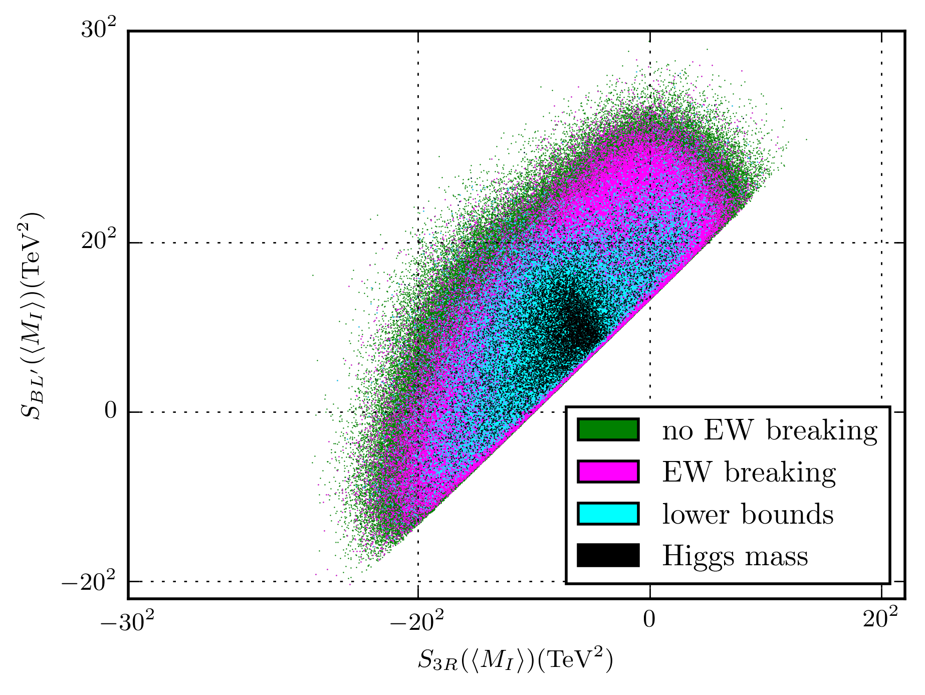
We now want to search for physically acceptable initial data, subject to all of the constraints and phenomenological conditions introduced above. Before applying any of these constraints, the number of parameters appearing in the MSSM greatly exceeds 100. However, subject to the constraints discussed above, this number is significantly reduced– down to only 24 soft SUSY breaking parameters, as well as and . The RG code Ovrut:2015uea that we use in this analysis involves all 24 SUSY breaking parameters. It is, however, helpful to point out that many of the RGE’s are dominated by two specific sums of these parameters given by
| (4.7) | |||
| (4.8) |
where the traces are over generational indices. This is helpful in that one can now reasonably plot initial data points in two-dimensional space, rather than in the full 24-dimensional space of all parameters. At the electroweak scale, we randomly set the value of . Furthermore, and importantly, we do not run the parameter . Rather, after running all other parameters down to the electroweak scale, we fine-tune to give the measured values for the electroweak gauge bosons, as discussed above.
Searching for physically acceptable initial data, subject to all of the constraints and phenomenological conditions above, we find the following. For 100 million sets of randomly scattered initial conditions, it is found that 4,351,809 break symmetry with the mass above the lower bound in equation (4.4). These are plotted as the green points in Figure 2. Running the RG down to the EW scale, one finds that of these 4,351,809 appropriate initial points, only 3,142,657 break electroweak symmetry with the experimentally measured values for and given in equation (4.5). These are shown as the purple points in the Figure. Now applying the constraints that all sparticle masses be at or above their currently measured lower bounds presented in Table 1, we find that of these 3,142,657 initial points, only 342,236 are acceptable. These are indicated by cyan colored points in the Figure. Finally, it turns out that of these 342,236 points, only 67,576 also lead to the currently measured Higgs mass given in equation (4.6). That is, of the 100 million sets of randomly scattered initial conditions, 67,576 satisfy all present phenomenological requirements. In Figure 2, we represent these “valid” points in black. That is, of the 100 million randomly scattered initial points, approximately .067% satisfy all present experimental conditions. Although this might– at first sight –appear to be a small percentage, it is worth noting that these initial points not only break symmetry appropriately and have all sparticle masses above their present experimental lower bounds, but also give the measured experimental values for the mass of the EW gauge bosons and, remarkably, the Higgs boson mass as well! From this point of view, this percentage of valid black points seems remarkably high. The electroweak gauge boson masses were obtained, as discussed above, by fine-tuning the parameter . For example, a typical value of the fine-tuning of is of the order of 1 in 1000 Ovrut:2014rba . However, one might also be concerned that getting the Higgs mass correct might require some other fine-tuning of the 24 initial parameters that may not be apparent. However, in previous work Ovrut:2015uea it was shown that the 24 parameters associated with any given black point are generically widely disparate with no apparent other fine-tuning.
We conclude that the MSSM, in addition to arising as a vacuum of heterotic M-theory and having exactly the mass spectrum of the MSSM, satisfies all present experimental low-energy physical bounds for a remarkably large number of disparate initial data points. Given this, it becomes of real interest to determine whether the RPV decays of the MSSM can be directly observed at the LHC at CERN. These decays are most easily observed in the lightest sparticles in the mass spectrum; that is, the LSP has the best prospects for RPV detection in general. There are, however, cases in which the next lightest supersymmetric particle (NLSP) is highly degenerate in mass with the LSP– see examples presented in Ovrut:2015uea –and, hence, their RPV decay channels become relevant as well. Hence, in the sections to follow, we compute the decays of charginos and neutralinos without making any assumptions regarding their masses. As discussed in detail in Ovrut:2015uea , the particle spectrum of each of the 67,576 valid black points is exactly determined by the computer code. It follows that we can compute the LSP associated with each valid black point. It turns out that there are many possible different LSPs. Before enumerating these, however, we must be more specific about the definition and structure of any LSP. Although the original fields entering the MSSM Lagrangian are “gauge” eigenstates, the LSP associated with a given valid black point is, by definition, a “mass” eigenstate– generically a linear combination of the original fields. For example, as will be discussed in detail in subsection 5.1, the lightest mass eigenstate chargino of either charge, which we denote by , is found to be an -parity conserving linear combination of the charged Wino, , and the charged Higgsino, , added to RPV terms proportional to the left and right chiral charged leptons. As discussed in subsection 5.1, the RPV coefficients are very small and, hence, can be ignored in the discussion of the masses of the charginos. Therefore, in this section, since we are analyzing the possible LSPs, we will consider the -parity conserving part of the chargino states only. It then follows from the discussion in subsection 5.1 that when the lightest chargino is given by
| (4.9) |
whereas for
| (4.10) |
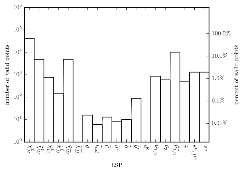
The angles are exactly determined for any given black point. It follows that for some black points the mass eigenstate is predominantly a charged Wino, whereas for other black points it is mainly a charged Higgsino. We will, henceforth, denote the first and second type of mass eigenstates by and , and refer to them as “Wino charginos” and “Higgsino charginos” respectively. That is, instead of labelling a chargino LSP simply as , and counting the number of valid black points associated with it, we can be more specific– breaking the chargino LSP into two different types of states, and respectively, and counting the number of black points associated with each type individually. This gives additional information about the structure of the LSPs.
With this in mind, we have calculated the LSP associated with each of the 67,576 valid black points and plotted the results as a histogram in Figure 3. The notation for the various possible LSPs is specified in Table 2. For example, out of the 67,576 valid black points, there are 4,858 that have a Wino chargino as their LSP. Similarly, out of all the valid black point initial conditions, 4,869 have a Wino neutralino as their LSP. And so on. Notice that the cases in which the chargino LSP is dominantly a charged Higgsino– that is, –are rare. In fact, in Figure 3 there is precisely one such black point. As discussed above and shown in Section 5, the lighter chargino state is dominantly Wino if , and dominantly Higgsino if . The little hierarchy problem tells us that is generally large, of the order of a few TeV. However, the parameter generally takes smaller values in our simulation. For this reason, the instances in which – required for the Higgsino chargino to be the LSP –are scarce.
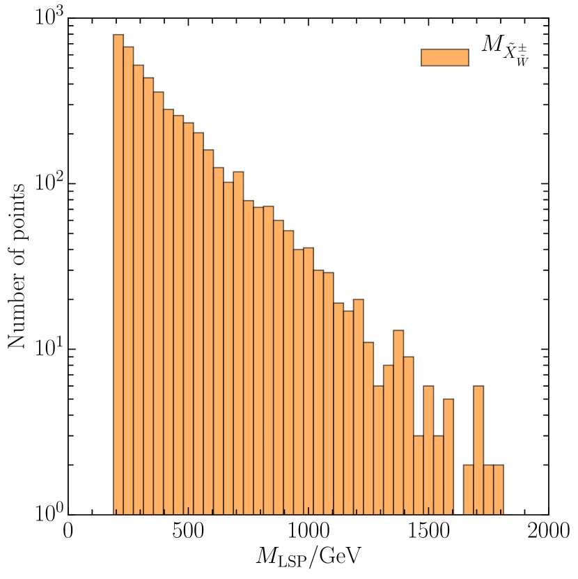
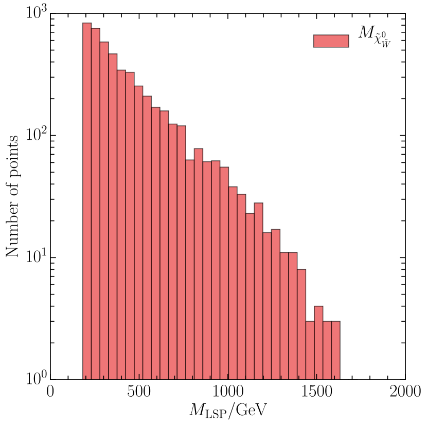
For any given choice of LSP, we can plot the number of such points as a function of their masses in GeV. As an example, Figures 4 (a) and (b) present such a mass distribution for Wino chargino and Wino neutralino LSPs respectively. We obtain viable supersymmetric spectra with Wino chargino and Wino neutralino LSP masses ranging from about 200 GeV to 1700 GeV. A striking feature of the Wino chargino and Wino neutralino LSP mass distributions in Figure 4 is the peak towards the low mass values. Higher LSP masses are exponentially less probable. The reason is that we sample all soft mass terms log-uniformly in the interval GeV, TeV]. This includes the gaugino mass term, which gives the dominant contribution for both the Wino chargino and Wino neutralino masses, see (5.6) and (5.47) respectively. If we would plot all the Wino chargino or Wino neutralino masses for all the viable points in our simulation, we would obtain an almost uniform mass distribution. However, for the Wino charginos or Wino neutralinos to be the LSPs, their masses must be lower than all the other random soft masses in our simulation. Conversely, it demands that all the other random soft mass terms be larger than a Wino chargino or Wino neutralino mass value for each viable point. This is exponentially less likely as this mass value increases, following a Boltzmann distribution. We point out that this discussion is a simplification of what actually happens, since it omits the running of the soft mass terms, as well as their mixing in the final mass eigenstates. These details, however, do not effect the essence of the above argument, since the mass runnings and the mass mixing couplings are generically very small.
Associated with a given choice of LSP, there are a fixed number of valid initial points. For example, as mentioned above, a Wino chargino LSP arises from 4,858 black points. As discussed at the end of Section 3, for each such black point, we 1) statistically throw one of the parameters in the interval GeV, 2) choose the neutrino mass hierarchy to be either normal or inverted and, having done so, choose the associated value of , 3) then, using (3.8), determine the remaining two epsilon parameters and the three parameters using the computer code. Let us denote the maximum one of the three parameters by . By running over all 4,858 black points subject to a fixed choice of the neutrino hierarchy and , one can create a histogram of the number of valid points associated with a given value for . For example, the results of, first, choosing a normal neutrino hierarchy and such that and, second, choosing an inverted neutrino hierarchy and with are graphically depicted in Figure 5.
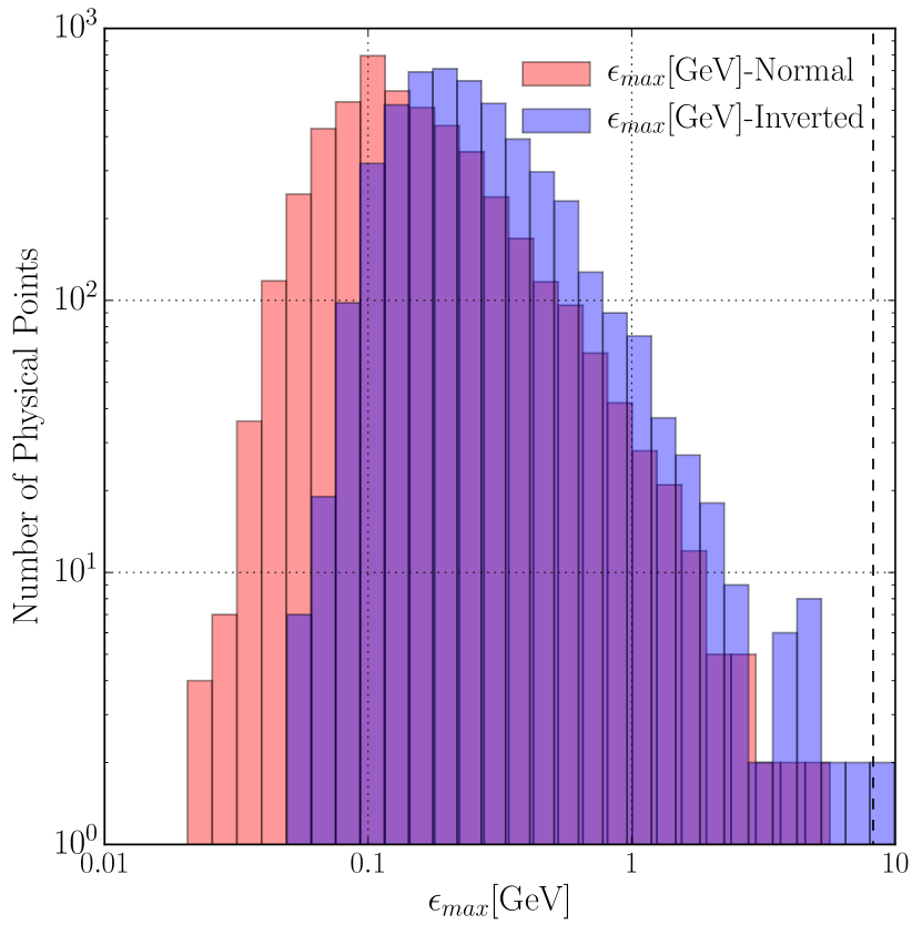
We find only a statistically insignificant number of points, in the case of the normal hierarchy 1 point and in the case of the inverted hierarchy 4 points, that exceed GeV. If , then constraint (3.22) is immediately satisfied. Even if this parameter is, say, , it remains statistically extremely likely that constraint (3.22) remains satisfied. It follows that, for the choice of a normal neutrino hierarchy and and an inverted hierarchy with , lepton number violation via is statistically highly suppressed in our theory. We find similar results for each of the other two choices of . The identical conclusion can be drawn for the Wino neutralino. We conclude that lepton number violation is highly suppressed in the MSSM– at least when the LSP is a Wino chargino or a Wino neutralino.
In previous papers Marshall:2014kea ; Marshall:2014cwa , we have analyzed in detail the RPV decays of the “admixture” stop. Stops have a very high production cross section from proton-proton collisions. Furthermore, their decay products are relatively easy to observe at the LHC detectors. For these reasons, the ATLAS group at the LHC did a detailed study of the RPV decays of the admixture stop LSPs Aaboud:2018wps ; ATLAS:2015jla ; Jackson:2015lmj ; ATLAS:2017hbw . However, it is clear from Figure 3 that neutralinos and charginos are much more prevalent as LSPs of the MSSM. Therefore, in the present paper, we begin a study of the RPV decays of neutralinos and charginos. Their RPV decay channels will be analyzed in detail.
| Symbol | Description |
|---|---|
| Mostly a neutral Bino. | |
| Mostly a neutral Wino. | |
| Mostly third generation right-handed neutrino. | |
| Mostly a neutral Higgsino. | |
| Mostly a charged Wino. | |
| Mostly a charged Higgsino. | |
| Gluino. | |
| Left- and right-handed stop admixture. | |
| Mostly right-handed stop (over 99%). | |
| Right-handed 1st and 2nd generation squarks. | |
| Mostly left-handed sbottom. | |
| Mostly right-handed sbottom. | |
| 1st and 2nd generation left-handed sneutrinos. | |
| LSPs evenly split among two generations. | |
| Third generation left-handed sneutrino. | |
| 1st and 2nd generation right-handed sneutrinos. | |
| Third generation left-handed stau. | |
| 1st and 2nd generation right-handed sleptons. | |
| LSPs evenly split among two generations. | |
| Third generation right-handed stau. |
5 Chargino and Neutralino states
5.1 Chargino mass eigenstates
After EW breaking, the Higgs fields acquire a VEV which induces off-diagonal couplings between the charged gauginos of the theory. The terms that enter the chargino mass matrix, in the absence of RPV effects, are
| (5.1) |
The first terms come from the supercovariant derivative of the Higgs chiral fields, the Wino mass term originates in the soft SUSY breaking Lagrangian, while the last term is introduced in the superpotential . Combining the charged Higgsinos and the charged Winos into and , we can write the previous terms in the form
| (5.2) |
where is the matrix given by
| (5.3) |
The mass eigenstates and diagonalize to
| (5.4) |
with and positive. One can solve analytically for the eigenvalues and obtain
| (5.5) |
where and correspond to the and sign in front of the square root respectively. We will always choose the square root to be positive, so that the "minus" sign– and, hence, –corresponds to the lighter mass eigenstate. That is, with this convention . The expressions for the mass eigenvalues can be simplified by noting that the lower bounds on sparticle masses are well above . It follows that . Therefore, the mass eigenvalues depend primarily on the parameters and . When , we find that
| (5.6) |
| (5.7) |
whereas for , the expressions for the mass eigenvalues are simply exchanged; that is,
| (5.8) |
| (5.9) |
The mixing matrices and , defined by
| (5.10) |
also are dependent on the relative sizes of and . For they are found to be
| (5.11) |
where
| (5.12) |
The Pauli matrix is inserted so that the diagonal entries of are always positive. The angles are given by
| (5.13) |
| (5.14) |
respectively. On the other hand, when , we find that (5.11) remains the same, as do the expressions (5.13) and (5.14) for the angles . However, the matrix now becomes
| (5.15) |
It is important to note that the results for the , matrices can be obtained from the expressions (5.11), (5.12), (5.13) and (5.14) simply by replacing
| (5.16) |
in all expressions. We will use this replacement, when required, in the main numerical analysis to follow.
It is useful to note that when , it follows from (5.12) that the lightest chargino eigenstate is
| (5.17) |
Since , we see from (5.13) and (5.14) that and, hence, . It follows that
| (5.18) |
We say that is “predominantly” a charged Wino and, regardless of the exact value of , denote it by . On the other hand, when it follows from (5.15) that
| (5.19) |
Expressions (5.13) and (5.14) again tell us that and, hence
| (5.20) |
That is, is “predominantly” a charged Higgsino and, regardless of the exact value of , we denote it by . Having made this analysis, we note that the results could have been read off directly from the leading term in the expressions for the mass eigenvalues given in (5.6) and (5.8). Specifically, for , the leading term in (5.6) is , the soft mass associated with the charged Wino– indicating that . Similarly, for , the leading term in (5.8) is , the parameter associated with the charged Higgsino– indicating that , as above. As stated previously, we will refer to the mass eigenstates and simply as a Wino chargino and Higgsino chargino respectively, even though they are only “predominantly” the pure states of and respectively.
Let us now include the -parity violation terms in the Lagrangian. These will not significantly affect the chargino masses, but they do introduce mixing between the charginos and the standard model charged leptons. These mixings are central to our study because they allow RPV chargino decays. In the extended bases and , the mixing matrix can again be written in the form of eq. (5.2),
| (5.21) |
now, however, where
| (5.22) |
and , , and denote the Dirac masses of the standard model charged leptons. This matrix can be expressed in a schematic form that will be useful in diagonalizing it. Let us write
| (5.23) |
where
| (5.24) |
and is the matrix with diagonal entries . The , , and matrices have entries that are much smaller than the entries of the matrix and, therefore, can be used to perturbatively diagonalize the matrix. The mass eigenstates are related to the gauge eigenstates by unitary matrices and defined by
| (5.25) |
They are chosen so that
| (5.26) |
where all eigenvalues are positive. The first two eigenstates, , are mostly charged Wino and charged Higgsino. The RPV couplings are small enough that their masses are still given by eqs. (5.6) and (5.7) or (5.8) and (5.9), depending on the values of the parameters and . Similarly, the masses of the leptons are basically unchanged; that is, are the standard model charged lepton masses, , where . The phenomenologically important effect of the RPV mixing is the RPV decays of the charginos. The matrices and can be written schematically as
| (5.27) |
Next, requiring that is diagonal allows one to compute the and matrices. To first order, they are given by
| (5.28) |
The values of all the and matrix elements are presented in the Appendix B.1. These matrices will be crucial in calculating the decay rates of the charginos via RPV processes. In general, the exact expressions for the five charged mass eigenstates are complicated, and will be dealt with numerically in our calculations. However, it of interest to present the complete analytic expressions, including the RPV terms, for the mass eigenstates . We find that the positive eigenvector is
| (5.29) |
where one sums over . When , the coefficients are given by
| (5.30) |
and
| (5.31) |
The result for is found by replacing in these expressions, as discussed above. Similarly, the negative eigenvector is found to be
| (5.32) |
where one sums over . When , the coefficients are given by
| (5.33) |
and
| (5.34) |
The result for is found by replacing in these expressions. Note that the first two terms of are independent of RPV and are identical to the expressions given in (5.17) and (5.19) for and respectively. Also, note that these terms dominate over the RPV terms and, hence, are the main contributors to the mass eigenvalues. However, although they are numerically smaller, the RPV terms in play a crucial role in the -parity violating decays of chargino LSPs and, hence, cannot be ignored.
5.2 Neutralino mass eigenstates
In the absence of the RPV violating terms proportional to and , the neutral Higgsinos and gauginos of the theory mix with the third generation right handed neutrino. In the gauge eigenstate basis ,
| (5.35) |
where
| (5.36) |
The mass eigenstates are related to the gauge states by the unitary matrix where . is chosen so that
| (5.37) |
where all eigenvalues are positive. The MSSM does not explicitly contain a Bino, associated with the hypercharge group . Instead, it contains a Blino and a Rino, the gauginos associated with and respectively. Nevertheless, the theory does effectively contain a Bino. To see this, consider the limit — that is, when the EW scale is much lower than the soft breaking scale so that the Higgs VEV’s are negligible. In this limit, the mass matrix in eq. (5.36) becomes
| (5.38) |
The first, fifth, and sixth columns, corresponding to the Blino, the Rino and the third generation right-handed neutrino, are now decoupled from the others and mix only with each other. In the reduced basis , the mixing matrix is
| (5.39) |
The limit in which the gaugino masses are much smaller than is phenomenologically relevant due to the lower bound on being much higher than typical gaugino mass lower bounds. This limit is also motivated theoretically because RG running makes the gauginos masses lighter. In this limit, the mass eigenstates can be found as an expansion in the gaugino masses. At zeroth order, they are
| (5.40) |
| (5.41) |
| (5.42) |
with masses, calculated to first order, given by
| (5.43) |
respectively. The state with mass is effectively a Bino. We can rotate from the old basis, , to the new one, , using a rotation matrix, which at zeroth order has the form:
| (5.44) |
We then get a new neutralino mass matrix, which is in agreement with the MSSM model after B-L breaking. It is given by
| (5.45) |
Since the EW scale is generally much lower than the gaugino mass scale, the off-diagonal terms are small,
| (5.46) |
| (5.47) |
| (5.48) |
| (5.49) |
| (5.50) |
| (5.51) |
where is the Weinberg angle. Unlike for charginos discussed previously, our labels do not imply any mass ordering. The exact eigenstates are more difficult to compute than in the chargino case. They are, generically, linear combinations of the six gauge neutralino states. However, as was discussed in detail for charginos, the dominant gauge neutralino in an eigenstate can be read off directly from the leading term in the associated mass eigenvalue. Using this, as well as explicit numerical computation, we find that
| (5.52) |
As with the charginos, we henceforth denote these mass eigenstates by , , , , , respectively; and refer to them as a Bino neutralino, a Wino neutralino and so on, even though they are only “predominantly” the pure neutral state.
Let us now add the RPV couplings and . This introduces mixing between the neutralinos and the neutral fermions of the standard model — the neutrinos. As discussed at the beginning of Section 3, mixing with the first- and second-family right-handed neutrino would lead to active-sterile neutrino oscillations. Unless and until there is more experimental evidence of such oscillations, we will continue to assume that they do not exist and, therefore, that the mixing with the first- and second-family right-handed neutrinos is negligible. Therefore, the neutrino mass matrix given below includes only mixing with the three families of left-handed neutrinos– the seventh column –and the third-family right-handed neutrino– the sixth column. As in the case of the charginos, the effect of adding these RPV couplings is important because it will allow RPV decays of the neutralinos. It’s effect on the physical masses of the neutralinos, however, is negligible. The new basis is then extended to . The extended mass matrix is given by
| (5.53) |
This is the matrix that was introduced in eq. (3.1). Just as for charginos, we can write the neutralino matrix in a schematic form that will help us diagonalize it perturbatively. As discussed in detail in Section 3, can be expressed as
| (5.54) |
where and are given in (3.2) and (3.3) respectively. The mass eigenstates are related to the gauge eigenstates by the unitary matrix , which diagonalizes the neutralino mixing matrix
| (5.55) |
can be written in the perturbative form
| (5.56) |
where is the unitary matrix introduced below eq. (5.36). It is a matrix, analogous to the matrices and in Section 5.1. However, while eq. (5.11), (5.12) and (5.15) provide simple analytic expressions for and in terms of the rotation angles , it is much harder to solve for without approximations. In this paper, we will compute numerically, using the the relevant soft mass terms and couplings as input.
The equation is obtained by requiring that be diagonal. We denote the mass eigenstates as . The entries of are central in calculating the neutralino decay rates and are all presented in Appendix B. However, exactly as in the case of the charginos discussed above, the physical masses of the “proper” neutralinos are not significantly changed by introducing the RPV couplings, so eqs. (5.46) – (5.51) remain valid. The states for are the three left-handed neutrinos which now receive Majorana masses. This process has been discussed in detail in Section 3. As in the case of charginos, it is important to note that, although small compared to the -parity preserving coefficients, the RPV terms make important contributions to the RPV decays of the neutralino LSPs and, hence, cannot be ignored.
6 Chargino and neutralino decay channels
6.1 General B-L MSSM Lagrangian
The general MSSM Lagrangian, written in terms of chiral multiplet component fields, (), and vector multiplet components, (), has the generic form
| (6.1) |
The interaction vertices that allow the charginos and neutralinos to decay into standard model particles are encoded in its complicated interactions. In order to read these RPV vertices from this Lagrangian, one needs to follow a series of steps:
- •
-
•
In the first step, the component fields are pure gauge states. After and electroweak symmetry breaking, these states mix to form massive states. In Section 5, we discussed how massive chargino and neutralino states are constructed. The second step then, is to write all gauge eigenstates in the Lagrangian in terms of their mass eigenstate expansion.
-
•
After the second step is completed, one can identify the RPV vertices that couple a single chargino or a single neutralino to two standard model particles, typically a boson and a lepton. However, so far the theory has been written in terms of 2-component Weyl spinors, while the physical fermions are described by 4-component spinors. The final step, then, is to write the identified RPV vertices in 4-component spinor notation.
In the following sections, we will identify the RPV decay amplitudes for the charginos and neutralinos displayed in Table 3, using the three steps described above. We find that such sparticle decays are due entirely to the RPV couplings proportional to and , that mix the three generations of leptons and the gauginos of the MSSM inside the chargino and neutralino mass matrices. That is, the mass eigenstate charginos and neutralinos can decay into SM particles precisely because they have lepton components. Only after we express the MSSM Lagrangian in terms of the mass eigenstates, will the decay processes in Table 3 become apparent. Henceforth, we use when referring to chargino and neutralino 2-component Weyl fermions and when referring to chargino and neutralino 4-component Dirac fermions. Furthermore, we use for the three families of charged leptons Weyl fermions, and for the three families expressed as Dirac fermions. The Dirac fermion states are defined in eq. (6.32).
| Charginos | Neutralinos |
|---|---|
6.2 Mass eigenstate expansion
The chargino mass eigenstates are related to the gauge eigenstates and via the unitary matrices and defined in Section 5 and given in Appendix B.1 . That is,
| (6.2) |
There are two things worth pointing out here. First, only the mass eigenstates and are considered to be the actual charginos. They have dominant contributions from the MSSM gauginos and only small SM lepton components. Moreover, the mass eigenstates , , are considered to be the three generations of charged leptons (to be more precise, the left-handed Weyl spinors of the negatively and positively charged leptons). Second, the and matrices are defined so that the chargino states are lighter than the chargino states ; that is, . The state can be dominantly charged Wino or charged Higgsino, but it will be always be less massive than .
In terms of the chargino mass eigenstates, the gauge eigenstate can be expressed as and . We then have the following mass eigenstate decomposition:
| (6.3) |
| (6.4) |
Similarly, the Wino and Higgsino gauge eigenstate can be expressed as:
| (6.5) |
| (6.6) |
| (6.7) |
| (6.8) |
The neutralino mass eigenstates are related to the gauge eigenstates via the unitary matrix , defined in Section 5 and given in Appendix B.2. That is,
| (6.9) |
Just as for the chargino states, it is important to remember that only the first six states are considered actual MSSM neutralinos, since their dominant contributions are from sparticles. The states are the three generations of left handed neutrinos, which obtain Majorana masses after the neutralino matrix diagonalization. However, the notation of the six neutralino mass eigenstates differs from that of the chargino mass eigenstates. In the case of charginos, the states are defined such that , where both and could be dominantly charged Wino or charged Higgsino. As discussed above, usually , in which case would be dominantly charged Wino, while would be dominantly charged Higgsino. In the rare case when , would be dominantly charged Higgsino, while would be dominantly charged Wino. For the neutralino mass eigenstates, however, we always have mostly Bino, mostly Wino, mostly Higgsino, mostly right-handed third generation neutrino. We don’t know, a priori, which state is the lightest, nor how to order them in terms of mass. Their masses are computed after we diagonalize the neutralino mixing matrix – neglecting RPV couplings –an operation significantly more complicated than the diagonalization of the chargino mass matrix, , in the absence of RPV couplings.
In terms of the neutralino mass eigesntates, the gauge eigenstates are given by
| (6.10) |
For the three neutrino gauge eigenstates
| (6.11) |
while for the rest of the mass eigenstates, we have
| (6.12) |
The Higgs scalar fields in the MSSM consist of two complex doublets; that is, eight degrees of freedom. When electroweak symmetry is broken, three of them become the Goldstone bosons , where . The rest will be Higgs scalar mass eigenstates; that is, CP-even neutral scalars and , a CP-odd neutral scalar and a charged and a conjugate . They are defined by Martin:1997ns .
| (6.13) |
| (6.14) |
where are rotation matrices. Specifically, the matrix in front of the Standard Model Higgs Boson is
| (6.15) |
while, to lowest order, the other matrices are
| (6.16) |
where . The mixing angle is, at tree level:
| (6.17) |
where the masses of the Higgs eigenstates are
| (6.18) |
| (6.19) |
and
| (6.20) |
6.3 Interaction vertices
We now express Lagrangian (6.1) in terms of all the matter and gauge fields in our MSSM theory, and then replace all gauge eigenstates with their mass eigenstate expansion. However, the full MSSM Lagrangian is complicated when expressed in its most general form. We proceed, therefore, by looking only for the terms that can lead to chargino or neutralino decays into standard model particles. We identify the following tri-couplings:
-
•
, from the covariant derivative of the fermionic matter fields
-
•
and , from the supercovariant derivatives
-
•
, from the gauge self-interaction
-
•
and , from the superpotential Yukawa couplings
We now want to write these interactions in terms of the MSSM component fields. The procedure is non-trivial. Hence, we split these interactions terms into two categories : 1) those responsible for the neutralino or chargino decays into a gauge boson (-boson or -boson) and a lepton; that is
| (6.21) |
and 2) those responsible for the decays into a Higgs boson and a lepton; that is
| (6.22) |
The terms with Yukawa couplings and those from the supercovariant derivatives are relevant only for the Higgs boson-lepton decay channel, as we will show.
6.3.1 -lepton
The part of the Lagrangian responsible for the gauge boson-lepton decay channels is
| (6.23) |
where this expression represents the sum over and . The represents the three lepton families. Expressed in terms of the MSSM component fields this becomes
| (6.24) |
where we sum over the index, are the three vector bosons of the group and the vector boson of the hypercharge group. Here, and are the and couplings. In addition, represents the -th left chiral lepton doublet defined in (2.13). We now make the replacements
| (6.25) |
where is the Weinberg angle, and rearrange the previous expression to obtain
| (6.26) |
, and are the usual weak charged, neutral and electromagnetic currents from the standard model theory of EW breaking, while , and are the equivalent currents of the Higgsino fermionic fields. Also note that is the electromagnetic coupling In 2-component Weyl notation these currents are:
-
•
Weak charged currents, coupling to bosons
(6.27) -
•
Electromagnetic currents, coupling to the photon
(6.28) -
•
Neutral currents, coupling to the boson
(6.29) (6.30)
where in , and we sum over . Plugging these currents into eq. (6.26), and arranging the couplings in terms of , and respectively, we get
| (6.31) |
where we have used the notation , and summed over .
Finally, we are in a position to expand all gauge eigenstates in terms of the mass eigenstates, as in equations (6.3)-(6.8) and (6.11)-(6.12). After this procedure, the Lagrangian (6.31) is expressed in terms of the mass eigenstates , , , for , and their hermitian conjugates. Notice that we keep only to simplify our results, since are always lighter than and, hence, have better prospects to be detected. Their charged Wino and charged Higgsino content are determined from the rotation matrices and in eq. (5.11). At the same time, we study the vertices of general neutralino states for , since we have no a priori mass ordering for these states. We remind the reader that means a mostly Bino neutralino , means a mostly Wino neutralino , means a mostly Higgsino neutralino and means a mostly third generation right-handed neutrino neutralino .
Until now, we have used 2-component Weyl spinor notation for all of our matter fields. Since we are interested in the decays of physical particles, we will henceforth introduce and use 4-component spinor notation for the initial and final states of the interacting particles. The 4-component spinors are defined in terms of the 2-component Weyl spinors as
| (6.32) |
In our model, are Dirac fermions, while are Majorana fermions. Note that, for simplicity, we use the same symbol, , for both a Weyl and Majorana neutrino. The Lagrangian (6.31) then becomes
| (6.33) |
where we sum over all neutralino states , all lepton families and . and are the projection operators and respectively.
It is important to note, however, that the last terms in this expression–that is, those proportional to the photon –exactly cancel. This occurs because the unitary matrices and satisfy the identities
| (6.34) |
and
| (6.35) |
It follows that the amplitude for the decay channel vanishes. Therefore, charginos cannot decay into a photon and a lepton
6.4 -lepton
The part of the Lagrangian responsible for the Higgs boson-lepton decay channels is
| (6.36) |
where this expression represents the sum over and . The index sums over the three lepton families. The terms with Yukawa couplings arising from the MSSM superpotential enter the Lagrangian as
| (6.37) |
Notice that we have kept only the terms with neutral Higgs scalar components, since only those have a Higgs boson mass eigenstate component . Other terms responsible for this decay channel arise from the supercovariant derivatives of the Higgs fields of the type
| (6.38) |
in Lagrangian (6.36). For the MSSM, these produce the terms
| (6.39) |
It follows that the part of the Lagrangian responsible for the decays is the sum of the equations (6.37) and (6.39). Note that these expressions are written in terms of the gauge eigenstates. As in the previous section, we expand the gauge eigenstates in terms of the mass eigenstates , , , for , and their hermitian conjugates. Once this step is completed, we group the terms into 4-component spinors to get
| (6.40) |
where the angle is defined in equation (6.17) and we sum over all lepton families .
One now has the information required to compute the amplitude for each of the processes listed in Table 3. To do this, we need the exact expression for the vertex coefficient associated with each such process. These can be read off from the Lagrangians in Eqs. (6.3.1) and (6.40). For example, consider the the decay channel . Then it follows from (6.3.1) that the vertex coupling is
| (6.41) |
where
| (6.42) |
and
| (6.43) |
However, their form and derivations are somewhat cumbersome. With this in mind,we provide a series of diagrams to pictorially express the origin of the interaction terms in the Lagrangian.
6.5 Chargino decay diagrams
6.5.1
The vertices associated with positively charged chargino decays are shown in Figures LABEL:fig:X11 and LABEL:fig:X12. The vertices associated with the negatively charged chargino decays are the hermitian conjugates of those. The diagrams in Figure LABEL:fig:X11 are expressed in terms of gauge eigenstates written as 2-component Weyl spinors. The diagrams in Figure LABEL:fig:X12 are the Feynman diagrams of the same vertices, in terms of 4-component mass eigenstates.


 (b1)
(b1)
 (b2)
(b2)
 (b3)
(b3)
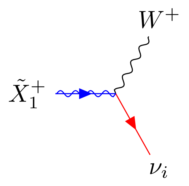 (b4)
(b4)
 (b5)
(b5)
(b)
6.5.2
The vertices associated with positively charged chargino decays are shown in Figures LABEL:fig:X21 and LABEL:fig:X22. The vertices associated with the negatively charged chargino decays are the hermitian conjugates of those. The diagrams in Figure LABEL:fig:X21 are expressed in terms of gauge eigenstates written as 2-component Weyl spinors. The diagrams in Figure LABEL:fig:X22 are the Feynman diagrams of the same vertices, in terms of 4-component mass eigenstates.


 (b1)
(b1)
 (b2)
(b2)
 (b3)
(b3)
 (b4)
(b4)
 (b5)
(b5)
 (b6)
(b6)
(b)
6.5.3
The vertices associated with positively charged chargino decays are shown in Figures LABEL:fig:X41 and LABEL:fig:X42. The vertices associated with the negatively charged chargino decays are the hermitian conjugates of those. The diagrams in Figure LABEL:fig:X41 are expressed in terms of gauge eigenstates written as 2-component Weyl spinors. The diagrams in Figure LABEL:fig:X42 are the Feynman diagrams of the same vertices, written in terms of 4-component mass eigenstates.


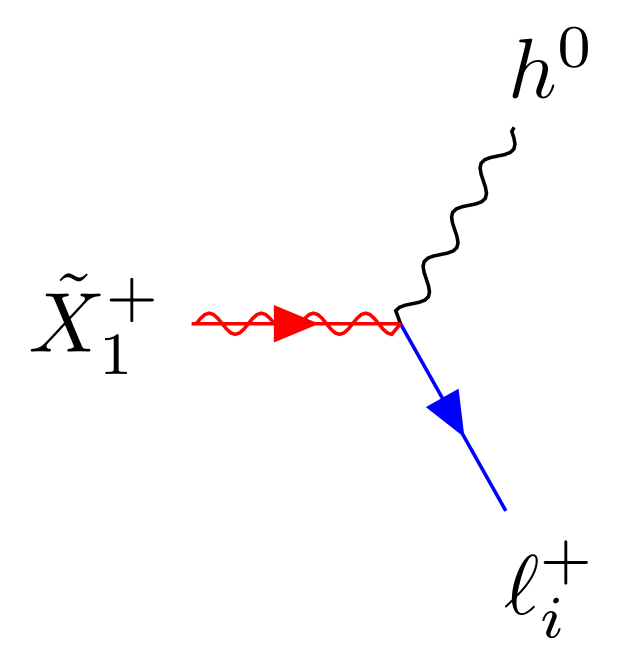 (b1)
(b1)
 (b2)
(b2)
 (b3)
(b3)
 (b4)
(b4)
 (b5)
(b5)
 (b6)
(b6)
(b)
6.6 Neutralino decay diagrams
6.6.1
The vertices associated with neutralino decays are shown in Figures LABEL:fig:X51 and LABEL:fig:X52. The diagrams in Figure LABEL:fig:X51 are expressed in terms gauge eigenstates written as 2-component Weyl spinors. The diagrams in Figure LABEL:fig:X52 are the same vertices in terms of mass eigenstates, expressed as 4-component spinors.


 (b1)
(b1)
 (b2)
(b2)
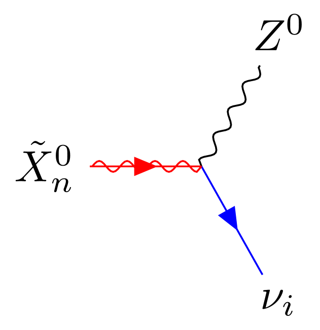 (b3)
(b3)
(b)
6.6.2
The vertices associated with neutralino decays are shown in Figures LABEL:fig:X61 and LABEL:fig:X62. The diagrams in Figure LABEL:fig:X61 are expressed in terms gauge eigenstates written as 2-component Weyl spinors. The diagrams in Figure LABEL:fig:X62 are the same vertices in terms of mass eigenstates, expressed as 4-component spinors.


 (b1)
(b1)
 (b2)
(b2)
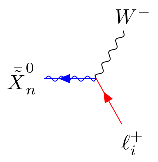 (b3)
(b3)
 (b4)
(b4)
 (b5)
(b5)
(b)
6.6.3
The vertices associated with neutralino decays are shown in Figures LABEL:fig:X71 and LABEL:fig:X72. The diagrams in Figure LABEL:fig:X71 are expressed in terms gauge eigenstates written as 2-component Weyl spinors. The diagrams in Figure LABEL:fig:X72 are the same vertices in terms of mass eigenstates, expressed as 4-component spinors.


 (b1)
(b1)
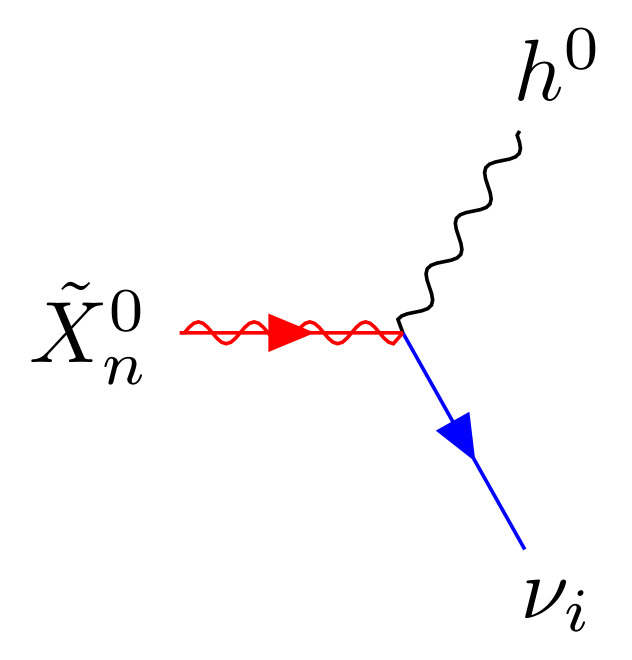 (b2)
(b2)
 (b3)
(b3)
 (b4)
(b4)
 (b5)
(b5)
(b)
7 Decay rates
In the previous discussion, we presented all relevant RPV decay channels of charginos and neutralinos into standard model particles and gave the associated Lagrangian interactions. In this section, we will use these results to calculate the decay rates associated with each such process. The calculations are carried out using the dominant linear terms in the RPV couplings and only, since higher order terms are highly suppressed. The analysis is completely general, regardless of whether or not the charginos or the neutralinos are the LSPs. However, only the lightest sparticles decay exclusively via RPV processes into SM particles. Furthermore, they have best prospects for detection at the LHC. Therefore, in subsequent publications, we will use these results to compute the RPV branching ratios of chargino and neutralinos LSPs and NLSPs.
7.1 Wino/Higgsino Chargino
We are ultimately interested in LSP and NSLP decays via RPV channels. Thus, we calculate the decay rates of the charginos only, which are defined to be lighter than the charginos. As discussed in detail at the end of subsection 5.1, a chargino mass eigenstate is a superposition of a charged Wino, a charged Higgsino and an RPV sum over left-chiral and right-chiral charged leptons gauge eigenstates.
In the present analysis, we will consider the decays of a generic chargino with arbitrary mixed charged Wino, charged Higgsino and RPV charged lepton content. More specialized decays involving predominantly Wino chargino or Higgsino chargino mass eigenstates, will be considered in future publications.
-
•
The terms in the Lagrangian associated with these decay channels have been calculated in eq. (6.3.1) and illustrated in Figure 6. Summing all the vertices, one finds
(7.1) and
(7.2) Next, using the expressions for the matrix elements of , and given in Appendices B.1 and B.2, we get
(7.3) and
(7.4) The decay width is proportional to the square of the amplitude of this process. Note that we account for the longitudinal degrees of freedom of the resultant gauge bosons (Goldostone equivalence theorem) in calculating this decay width. This results in an amplification of this channel, which becomes more significant as the mass of the decaying chargino increases. The result is
(7.5) Note that and are proportional to the RPV couplings and at first order. Therefore, the decay of the chargino into the SM particles boson and neutrino would vanish in the absence of RPV.
-
•
The terms in the Lagrangian associated with these decay channels have been calculated in eq. (6.3.1) and illustrated in Figure 7. Summing all the vertices, one finds
(7.6) and
(7.7) Using the expressions for the matrix elements of and from the Appendix B.1, we get
(7.8) and
(7.9) where there is no sum over the in .
The decay width is proportional to the square of the amplitude of this process. We note that we have accounted for the longitudinal degrees of freedom of the resultant gauge bosons (Goldstone equivalence theorem) in calculating this decay width. This results in an amplification of this channel which becomes more significant as the mass of the decaying chargino increases. We find that
(7.10) Note that both coefficients are proportional to the RPV couplings and at first order. Therefore, there would be no decay of the chargino into the SM boson and charged leptons if the RPV effects were non-existent.
-
•
The terms in the Lagrangian associated with these decay channels have been calculated in eq. (6.40) and illustrated in Figure 8. Summing all the vertices, one finds(7.11) and
(7.12) Next, using the expressions for the matrix elements of and from the Appendix B.1, we get
(7.13) and
(7.14) where we do not sum over the in either of these expressions. The decay width is proportional to the square of the amplitude of this process, and is found to be
(7.15) Again, note that are proportional to the RPV couplings and at first order. Hence, there would be no decay of the chargino into the SM Higgs boson and charged leptons if there would be no RPV effects.
7.2 Neutralinos
Recall that the index indicates the neutralino species as follows:
| (7.16) |
For a general neutralino state , we found expressions for the parameters of the decay to two standard model particles.
Note that in the above neutralino expressions, we sum over . Using the matrix elements of , and given in Appendices B.1 and B.2, one can can calculate the values of the decay rates numerically. Just as for charginos, it can be shown that the decay amplitudes are proportional to the RPV couplings and at first order. Hence, RPV is directly responsible for the neutralino decays into SM particles.
Acknowledgments
The authors would like to thank Evelyn Thomson, Elliot Lipeles, Jeff Dandoy, Christopher Mauger, Nuno Barros, Leigh Schaefer, and Christian Herwig for helpful suggestions. Ovrut and Purves would also like to acknowledge many informative conversations with Zachary Marshall and Sogee Spinner concerning RPV decays of a stop LSP. Burt Ovrut and Sebastian Dumitru are supported in part by DOE No. DE-SC0007901 and SAS Account 020-0188-2-010202-6603-0338.
Appendix A Notation
In this Appendix, we present for clarity all the notation used throughout the paper.
A.1 Gauge Eigenstates
-
•
Bosons
vector gauge bosons
, coupling parameter
, coupling parameter
, coupling parameter
, coupling parameter
, coupling parameter
B-L Breaking: massive boson , coupling
EW Breaking: massive bosons
Higgs scalars
-
•
Weyl Spinors
gauginos
, ,
Higgsinos
leptons
left chiral
right chiral
sleptons
left chiral
right chiral
A.2 Mass Eigenstates
-
•
Weyl Spinors
leptons
charginos and neutralinos
-
•
4-component Spinors
leptons
charginos and neutralinos
A.3 VEV’s
-
•
sneutrino VEV’s
-
•
Higgs VEV’s
Appendix B Mass Matrix elements
B.1 Chargino mass matrix
The matrices and can be written schematically as
| (B.1) |
Assuming that the lighter chargino is , and since we are interested in its decays, it follows that we will need the elements and and their conjugates when replacing a lepton state with the lightest chargino mass eigenstate. It follows from the above that
| (B.2) |
| (B.3) |
When replacing a charged Wino gaugino with the lightest chargino mass eigenstate, we need the elements and given by
| (B.4) |
and their conjugates. Similarly for replacing a charged Higgsino, one needs and , which we find to be
| (B.5) |
and their conjugates.
We also need the elements and and their complex conjugates when replacing a charged Wino state with a charged lepton, where
| (B.6) |
The elements and and their complex conjugates when required when replacing a charged Higgsino state with a charged lepton,
| (B.7) |
The angles are defined in Section 5.1. They express the charged Wino and charged Higgsino content of the chargino mass eigenstates, in the absence of the RPV couplings and
| (B.8) |
and
| (B.9) |
Hence, for , we have purely Wino chargino states and purely Higgsino chargino states . Conversely, for , we have purely Higgsino chargino states and purely Wino chargino states .
B.2 Neutralino mass matrix
The matrix can be written schematically as
| (B.10) |
The rows of are the gaugino gauge eigenstates, whereas the columns correspond to the neutrino gauge eigenstates. These are explicitly labeled and presented below. They are
| (B.11) |
| (B.12) |
| (B.13) |
| (B.14) |
| (B.15) |
| (B.16) |
where
| (B.17) |
| (B.18) |
| (B.19) |
We can now express the matrix elements of
| (B.20) |
is the matrix that diagonalizes the neutralino mass matrix in the absence of RPV couplings to the three families of left-handed neutrinos. If the soft masses in the neutralino mass matrix, eq. (B.20), are much larger than the Higgs VEV’s and , then, at zeroth order, we have
| (B.21) |
However, in the regimes with small chargino and neutralino masses that we analyze, this approximation is no longer valid. The elements of will, in general, have complicated expressions and we choose to evaluate them numerically. We use as input the numerical values of the neutralino mass matrix. We expect, however, based on the zeroth order form of , that , , , , , , , , , and are of order , while the remaining matrix elements are of order .
Elements form the top-right block have the form
| (B.22) |
for and . Elements of the bottom left block are computed in a similar fashion. One can then determine as
| (B.23) |
References
- (1) G. Aad et al. [ATLAS Collaboration], “Observation of a new particle in the search for the Standard Model Higgs boson with the ATLAS detector at the LHC,” Phys. Lett. B 716, 1 (2012) doi:10.1016/j.physletb.2012.08.020 [arXiv:1207.7214 [hep-ex]].
- (2) S. Chatrchyan et al. [CMS Collaboration], “Observation of a new boson at a mass of 125 GeV with the CMS experiment at the LHC,” Phys. Lett. B 716, 30 (2012) doi:10.1016/j.physletb.2012.08.021 [arXiv:1207.7235 [hep-ex]].
- (3) D. J. Gross, J. A. Harvey, E. J. Martinec and R. Rohm, “The Heterotic String,” Phys. Rev. Lett. 54, 502 (1985). doi:10.1103/PhysRevLett.54.502
- (4) P. Horava and E. Witten, “Eleven-dimensional supergravity on a manifold with boundary,” Nucl. Phys. B 475, 94 (1996) doi:10.1016/0550-3213(96)00308-2 [hep-th/9603142].
- (5) A. Lukas, B. A. Ovrut and D. Waldram, “On the four-dimensional effective action of strongly coupled heterotic string theory,” Nucl. Phys. B 532, 43 (1998) doi:10.1016/S0550-3213(98)00463-5 [hep-th/9710208].
- (6) A. Lukas, B. A. Ovrut and D. Waldram, “The Ten-dimensional effective action of strongly coupled heterotic string theory,” Nucl. Phys. B 540, 230 (1999) doi:10.1016/S0550-3213(98)00684-1 [hep-th/9801087].
- (7) A. Lukas, B. A. Ovrut, K. S. Stelle and D. Waldram, “The Universe as a domain wall,” Phys. Rev. D 59, 086001 (1999) doi:10.1103/PhysRevD.59.086001 [hep-th/9803235].
- (8) A. Lukas, B. A. Ovrut, K. S. Stelle and D. Waldram, “Heterotic M theory in five-dimensions,” Nucl. Phys. B 552, 246 (1999) doi:10.1016/S0550-3213(99)00196-0 [hep-th/9806051].
- (9) M. Evans and B. A. Ovrut, “Splitting the Superstring Vacuum Degeneracy,” Phys. Lett. B 174, 63 (1986). doi:10.1016/0370-2693(86)91130-5
- (10) R. Donagi, B. A. Ovrut, T. Pantev and D. Waldram, “Spectral involutions on rational elliptic surfaces,” Adv. Theor. Math. Phys. 5, 499 (2002) doi:10.4310/ATMP.2001.v5.n3.a4 [math/0008011 [math-ag]].
- (11) R. Donagi, Y. H. He, B. A. Ovrut and R. Reinbacher, “The Particle spectrum of heterotic compactifications,” JHEP 0412, 054 (2004) doi:10.1088/1126-6708/2004/12/054 [hep-th/0405014].
- (12) V. Braun, Y. H. He, B. A. Ovrut and T. Pantev, “Vector bundle extensions, sheaf cohomology, and the heterotic standard model,” Adv. Theor. Math. Phys. 10, no. 4, 525 (2006) doi:10.4310/ATMP.2006.v10.n4.a3 [hep-th/0505041].
- (13) V. Braun, Y. H. He, B. A. Ovrut and T. Pantev, “The Exact MSSM spectrum from string theory,” JHEP 0605, 043 (2006) doi:10.1088/1126-6708/2006/05/043 [hep-th/0512177].
- (14) L. B. Anderson, J. Gray, A. Lukas and B. Ovrut, “Stabilizing All Geometric Moduli in Heterotic Calabi-Yau Vacua,” Phys. Rev. D 83, 106011 (2011) doi:10.1103/PhysRevD.83.106011 [arXiv:1102.0011 [hep-th]].
- (15) E. I. Buchbinder, R. Donagi and B. A. Ovrut, “Vector bundle moduli superpotentials in heterotic superstrings and M theory,” JHEP 0207, 066 (2002) doi:10.1088/1126-6708/2002/07/066 [hep-th/0206203].
- (16) R. Donagi, B. A. Ovrut and D. Waldram, “Moduli spaces of five-branes on elliptic Calabi-Yau threefolds,” JHEP 9911, 030 (1999) doi:10.1088/1126-6708/1999/11/030 [hep-th/9904054].
- (17) E. Lima, B. A. Ovrut, J. Park and R. Reinbacher, “Nonperturbative superpotential from membrane instantons in heterotic M theory,” Nucl. Phys. B 614, 117 (2001) doi:10.1016/S0550-3213(01)00404-7 [hep-th/0101049].
- (18) L. B. Anderson, J. Gray, A. Lukas and B. Ovrut, “Stability Walls in Heterotic Theories,” JHEP 0909, 026 (2009) doi:10.1088/1126-6708/2009/09/026 [arXiv:0905.1748 [hep-th]].
- (19) L. B. Anderson, J. Gray, D. Grayson, Y. H. He and A. Lukas, “Yukawa Couplings in Heterotic Compactification,” Commun. Math. Phys. 297, 95 (2010) doi:10.1007/s00220-010-1033-8 [arXiv:0904.2186 [hep-th]].
- (20) S. Blesneag, E. I. Buchbinder, P. Candelas and A. Lukas, “Holomorphic Yukawa Couplings in Heterotic String Theory,” JHEP 1601, 152 (2016) doi:10.1007/JHEP01(2016)152 [arXiv:1512.05322 [hep-th]].
- (21) S. Blesneag, E. I. Buchbinder and A. Lukas, “Holomorphic Yukawa Couplings for Complete Intersection Calabi-Yau Manifolds,” JHEP 1701, 119 (2017) doi:10.1007/JHEP01(2017)119 [arXiv:1607.03461 [hep-th]].
- (22) V. Braun, Y. H. He and B. A. Ovrut, “Yukawa couplings in heterotic standard models,” JHEP 0604, 019 (2006) doi:10.1088/1126-6708/2006/04/019 [hep-th/0601204].
- (23) R. Deen, B. A. Ovrut and A. Purves, “The minimal SUSY B-L model: simultaneous Wilson lines and string thresholds,” JHEP 1607, 043 (2016) doi:10.1007/JHEP07(2016)043 [arXiv:1604.08588 [hep-ph]].
- (24) V. S. Kaplunovsky, “One loop threshold effects in string unification,” hep-th/9205070.
- (25) V. Kaplunovsky and J. Louis, “On Gauge couplings in string theory,” Nucl. Phys. B 444, 191 (1995) doi:10.1016/0550-3213(95)00172-O [hep-th/9502077].
- (26) P. Mayr, H. P. Nilles and S. Stieberger, “String unification and threshold corrections,” Phys. Lett. B 317, 53 (1993) doi:10.1016/0370-2693(93)91569-9 [hep-th/9307171].
- (27) K. R. Dienes, A. E. Faraggi and J. March-Russell, “String unification, higher level gauge symmetries, and exotic hypercharge normalizations,” Nucl. Phys. B 467, 44 (1996) doi:10.1016/0550-3213(96)00085-5 [hep-th/9510223].
- (28) K. R. Dienes, “String theory and the path to unification: A Review of recent developments,” Phys. Rept. 287, 447 (1997) doi:10.1016/S0370-1573(97)00009-4 [hep-th/9602045].
- (29) H. P. Nilles and S. Stieberger, “String unification, universal one loop corrections and strongly coupled heterotic string theory,” Nucl. Phys. B 499, 3 (1997) doi:10.1016/S0550-3213(97)00315-5 [hep-th/9702110].
- (30) D. M. Ghilencea and G. G. Ross, “Precision prediction of gauge couplings and the profile of a string theory,” Nucl. Phys. B 606, 101 (2001) doi:10.1016/S0550-3213(01)00234-6 [hep-ph/0102306].
- (31) S. P. de Alwis, “Gauge Threshold Corrections and Field Redefinitions,” Phys. Lett. B 722, 176 (2013) doi:10.1016/j.physletb.2013.04.007 [arXiv:1211.5460 [hep-th]].
- (32) D. Bailin and A. Love, “Reduced modular symmetries of threshold corrections and gauge coupling unification,” JHEP 1504, 002 (2015) doi:10.1007/JHEP04(2015)002 [arXiv:1412.7327 [hep-th]].
- (33) R. Deen, B. A. Ovrut and A. Purves, “Supersymmetric Sneutrino-Higgs Inflation,” Phys. Lett. B 762, 441 (2016) doi:10.1016/j.physletb.2016.09.059 [arXiv:1606.00431 [hep-ph]].
- (34) S. Ferrara and A. Sagnotti, “Supersymmetry and Inflation,” Int. J. Mod. Phys. 1, 29 (2017) doi:10.1142/9789813226609_0003 [arXiv:1509.01500 [hep-th]].
- (35) A. Linde, “On inflation, cosmological constant, and SUSY breaking,” JCAP 1611, no. 11, 002 (2016) doi:10.1088/1475-7516/2016/11/002 [arXiv:1608.00119 [hep-th]].
- (36) M. Koehn, J. L. Lehners and B. A. Ovrut, “Higher-Derivative Chiral Superfield Actions Coupled to N=1 Supergravity,” Phys. Rev. D 86, 085019 (2012) doi:10.1103/PhysRevD.86.085019 [arXiv:1207.3798 [hep-th]].
- (37) L. Battarra, M. Koehn, J. L. Lehners and B. A. Ovrut, “Cosmological Perturbations Through a Non-Singular Ghost-Condensate/Galileon Bounce,” JCAP 1407, 007 (2014) doi:10.1088/1475-7516/2014/07/007 [arXiv:1404.5067 [hep-th]].
- (38) Z. Marshall, B. A. Ovrut, A. Purves and S. Spinner, “LSP Squark Decays at the LHC and the Neutrino Mass Hierarchy,” Phys. Rev. D 90, no. 1, 015034 (2014) doi:10.1103/PhysRevD.90.015034 [arXiv:1402.5434 [hep-ph]].
- (39) M. Ambroso and B. Ovrut, “The B-L/Electroweak Hierarchy in Heterotic String and M-Theory,” JHEP 0910, 011 (2009) doi:10.1088/1126-6708/2009/10/011 [arXiv:0904.4509 [hep-th]].
- (40) M. Ambroso and B. A. Ovrut, “The B-L/Electroweak Hierarchy in Smooth Heterotic Compactifications,” Int. J. Mod. Phys. A 25, 2631 (2010) doi:10.1142/S0217751X10049207 [arXiv:0910.1129 [hep-th]].
- (41) M. Ambroso and B. A. Ovrut, “The Mass Spectra, Hierarchy and Cosmology of B-L MSSM Heterotic Compactifications,” Int. J. Mod. Phys. A 26, 1569 (2011) doi:10.1142/S0217751X11052943 [arXiv:1005.5392 [hep-th]].
- (42) B. A. Ovrut, A. Purves and S. Spinner, “Wilson Lines and a Canonical Basis of SU(4) Heterotic Standard Models,” JHEP 1211, 026 (2012) doi:10.1007/JHEP11(2012)026 [arXiv:1203.1325 [hep-th]].
- (43) B. A. Ovrut, A. Purves and S. Spinner, “A statistical analysis of the minimal SUSY B–L theory,” Mod. Phys. Lett. A 30, no. 18, 1550085 (2015) doi:10.1142/S0217732315500856 [arXiv:1412.6103 [hep-ph]].
- (44) B. A. Ovrut, A. Purves and S. Spinner, “The minimal SUSY B-L model: from the unification scale to the LHC,” JHEP 1506, 182 (2015) doi:10.1007/JHEP06(2015)182 [arXiv:1503.01473 [hep-ph]].
- (45) P. Fileviez Perez and S. Spinner, “Spontaneous -parity Breaking and Left-Right Symmetry,” Phys. Lett. B 673 (2009) 251 [arXiv:0811.3424 [hep-ph]].
- (46) V. Barger, P. Fileviez Perez and S. Spinner, “Minimal gauged U(1)(B-L) model with spontaneous -parity violation,” Phys. Rev. Lett. 102 (2009) 181802 [arXiv:0812.3661 [hep-ph]].
- (47) P. Fileviez Perez and S. Spinner “Spontaneous -parity Breaking in SUSY Models,” Phys. Rev. D 80, 01004 (2009) [arXiv:0904.2213 [hep-ph]]
- (48) L. L. Everett, P. Fileviez Perez and S. Spinner, “The Right Side of Tev Scale Spontaneous -parity Violation,” Phys. Rev. D 80 (2009) 055007 [arXiv:0906.4095 [hep-ph]].
- (49) P. Fileviez Perez and S. Spinner, “The Minimal Theory for -parity Violation at the LHC,” arXiv:1201.5923 [hep-ph].
- (50) P. Fileviez Perez and S. Spinner, “Supersymmetry at the LHC and The Theory of -parity,” Phys. Lett. B 728, 489 (2014) [arXiv:1308.0524 [hep-ph]].
- (51) S. P. Martin, “A Supersymmetry primer,” Adv. Ser. Direct. High Energy Phys. 21, 1 (2010) [Adv. Ser. Direct. High Energy Phys. 18, 1 (1998)] [hep-ph/9709356].
- (52) Z. Marshall, B. A. Ovrut, A. Purves and S. Spinner, “Spontaneous -Parity Breaking, Stop LSP Decays and the Neutrino Mass Hierarchy,” Phys. Lett. B 732, 325 (2014) doi:10.1016/j.physletb.2014.03.052 [arXiv:1401.7989 [hep-ph]].
- (53) M. Aaboud et al. [ATLAS Collaboration], “Search for B-L R -parity-violating top squarks in =13??TeV pp collisions with the ATLAS experiment,” Phys. Rev. D 97, no. 3, 032003 (2018) doi:10.1103/PhysRevD.97.032003 [arXiv:1710.05544 [hep-ex]].
- (54) R. Barbier et al., “R-parity violating supersymmetry,” Phys. Rept. 420, 1 (2005) doi:10.1016/j.physrep.2005.08.006 [hep-ph/0406039].
- (55) R. N. Mohapatra, “Supersymmetry and R-parity: an Overview,” Phys. Scripta 90, 088004 (2015) doi:10.1088/0031-8949/90/8/088004 [arXiv:1503.06478 [hep-ph]].
- (56) D. Dercks, H. Dreiner, M. E. Krauss, T. Opferkuch and A. Reinert, “R-Parity Violation at the LHC,” Eur. Phys. J. C 77, no. 12, 856 (2017) doi:10.1140/epjc/s10052-017-5414-4 [arXiv:1706.09418 [hep-ph]].
- (57) S. Dumitru, B. A. Ovrut and A. Purves, “-parity Violating Decays of Wino Chargino and Wino Neutralino LSPs and NLSPs at the LHC,” arXiv:1811.05581 [hep-ph].
- (58) P. Fundira and A. Purves, “Bayesian naturalness, simplicity, and testability applied to the MSSM GUT,” Int. J. Mod. Phys. A 33, no. 11, 1841004 (2018) doi:10.1142/S0217751X1841004X [arXiv:1708.07835 [hep-ph]].
- (59) G. Senjanovic and R. N. Mohapatra, “Exact Left-Right Symmetry and Spontaneous Violation of Parity,” Phys. Rev. D 12, 1502 (1975). doi:10.1103/PhysRevD.12.1502
- (60) W. Grimus, “Introduction to left-right symmetric models,” UWTHPH-1993-10.
- (61) B. Mukhopadhyaya, S. Roy and F. Vissani, “Correlation between neutrino oscillations and collider signals of supersymmetry in an -parity violating model,” Phys. Lett. B 443, 191 (1998) [hep-ph/9808265].
- (62) E. J. Chun and J. S. Lee, “Implication of Super-Kamiokande data on -parity violation,” Phys. Rev. D 60, 075006 (1999) [hep-ph/9811201].
- (63) E. J. Chun and S. K. Kang, “One loop corrected neutrino masses and mixing in supersymmetric standard model without -parity,” Phys. Rev. D 61, 075012 (2000) [hep-ph/9909429].
- (64) M. Hirsch, M. A. Diaz, W. Porod, J. C. Romao and J. W. F. Valle, “Neutrino masses and mixings from supersymmetry with bilinear R parity violation: A Theory for solar and atmospheric neutrino oscillations,” Phys. Rev. D 62, 113008 (2000) [Erratum-ibid. D 65, 119901 (2002)] [hep-ph/0004115].
- (65) D. K. Ghosh, G. Senjanovic and Y. Zhang, “Naturally Light Sterile Neutrinos from Theory of -parity,” Phys. Lett. B 698 (2011) 420 [arXiv:1010.3968 [hep-ph]].
- (66) V. Barger, P. Fileviez Perez and S. Spinner, “Three Layers of Neutrinos,” Phys. Lett. B 696 (2011) 509 [arXiv:1010.4023 [hep-ph]].
- (67) R. N. Mohapatra, “Mechanism For Understanding Small Neutrino Mass In Superstring Theories,” Phys. Rev. Lett. 56 (1986) 561.
- (68) G. Aad et al. [ATLAS Collaboration], “Searches for heavy long-lived charged particles with the ATLAS detector in proton-proton collisions at TeV,” JHEP 1501, 068 (2015) doi:10.1007/JHEP01(2015)068 [arXiv:1411.6795 [hep-ex]].
- (69) G. Aad et al. [ATLAS Collaboration], “Search for massive, long-lived particles using multitrack displaced vertices or displaced lepton pairs in pp collisions at = 8 TeV with the ATLAS detector,” Phys. Rev. D 92, no. 7, 072004 (2015) doi:10.1103/PhysRevD.92.072004 [arXiv:1504.05162 [hep-ex]].
- (70) M. Tanabashi et al. (Particle Data Group), Phys. Rev. D 98, 030001 (2018)
- (71) F. Capozzi, E. Lisi, A. Marrone and A. Palazzo, “Current unknowns in the three neutrino framework,” arXiv:1804.09678 [hep-ph].
- (72) M. Aaboud et al. [ATLAS Collaboration], “Search for new high-mass phenomena in the dilepton final state using 36 fb1 of proton-proton collision data at TeV with the ATLAS detector,” JHEP 1710, 182 (2017) doi:10.1007/JHEP10(2017)182 [arXiv:1707.02424 [hep-ex]].
- (73) M. Aaboud et al. [ATLAS Collaboration], “Measurement of the Higgs boson mass in the and channels with TeV collisions using the ATLAS detector,” arXiv:1806.00242 [hep-ex].
- (74) The ATLAS collaboration [ATLAS Collaboration], “A search for -Parity violating scalar top decays in TeV collisions with the ATLAS experiment,” ATLAS-CONF-2015-015.
- (75) B. Jackson, “A Search For -Parity-Violating Scalar Top Decays in TeV Collisions With The ATLAS Experiment,” CERN-THESIS-2015-129.
- (76) The ATLAS collaboration [ATLAS Collaboration], “A search for B-L R-parity-violating scalar tops in = 13 TeV collisions with the ATLAS experiment,” ATLAS-CONF-2017-036.