Fiducial polarization observables in hadronic WZ production: A next-to-leading order QCD+EW study

Abstract

We present a study at next-to-leading-order (NLO) of the process $pp\to W^{\pm}Z\to\ell\nu_{l}\ell^{\prime+}\ell^{\prime-}$, where $\ell,\ell^{\prime}=e,\mu$, at the Large Hadron Collider. We include the full NLO QCD corrections and the NLO electroweak (EW) corrections in the double-pole approximation. We define eight fiducial polarization coefficients directly constructed from the polar-azimuthal angular distribution of the decay leptons. These coefficients depend strongly on the kinematical cuts on the transverse momentum or rapidity of the individual leptons. Similarly, fiducial polarization fractions are also defined and they can be directly related to the fiducial coefficients. We perform a detailed analysis of the NLO QCD+EW fiducial polarization observables including theoretical uncertainties stemming from the scale variation and parton distribution function uncertainties, using the fiducial phase space defined by the ATLAS and CMS experiments. We provide results in the helicity coordinate system and in the Collins-Soper coordinate system, at a center-of-mass energy of 13 TeV. The EW corrections are found to be important in two of the angular coefficients related to the $Z$ boson, irrespective of the kinematical cuts or the coordinate system. Meanwhile, those EW corrections are very small for the $W^{\pm}$ bosons.

1 Introduction

Since the Large Hadron Collider (LHC) at CERN has started to operate, the production of electroweak gauge bosons has been extensively studied both by theorists and experimentalists. With the accumulation of data we can reach high precision measurements, thus probing new physics effects in non-trivial observables such as in the polarization of the gauge bosons. $W$ bosons only interact with left-handed quarks, while $Z$ bosons interact with both left- and right-handed quarks, but with different coupling strengths. This means that $W$ and $Z$ bosons produced at hadron colliders are in principle polarized and that the angular distributions of the final-state leptons display an asymmetry that reflects the polarization of the underlying gauge bosons.

The polarization of gauge bosons produced in hadron collider processes has been studied in the literature. At the LHC, $W$ bosons are produced abundantly in top quark decays or in association with jets, where the later channel is characterized by high transverse momentum $W$ bosons. The polarization of $W$ boson in the top quark decay has been measured by ATLAS Aad:2012ky and CMS Khachatryan:2016fky . For $W+\text{jets}$, polarization measurements have also been performed by CMS Chatrchyan:2011ig and ATLAS ATLAS:2012au . Similar studies for $Z$ boson polarization in $Z+\text{jets}$ channel have been presented by CMS Khachatryan:2015paa and ATLAS Aad:2016izn . Recent theoretical studies for $W+\text{jets}$ have been presented in Refs. Bern:2011ie ; Stirling:2012zt .

The study in Ref. Bern:2011ie uses the helicity coordinate system in which the angular observables for the $W$ boson are defined, namely the $W$ boson rest frame where the $z$ direction is defined as the direction of the $W$ boson in the laboratory frame. Another popular coordinate system has been previously introduced in Ref. Collins:1977iv , called the Collins-Soper coordinate system, in which the $z$ direction is defined as the bisection of the flight direction of the two incoming protons in the $W$ boson rest frame. It is noted that both ATLAS and CMS use the helicity coordinate system for $W+\text{jets}$ and Collins-Soper coordinate system for $Z+\text{jets}$. Following Ref. Collins:1977iv there has been a number of phenomenological studies of the spin-density matrix of the $W$ boson Lam:1980uc ; Mirkes:1992hu ; Aguilar-Saavedra:2015yza as well as of the $Z$ boson Mirkes:1994eb ; Aguilar-Saavedra:2017zkn , that relate to the corresponding angular coefficients. One-loop QCD effects have also been studied in Refs. Hagiwara:1984hi ; Hagiwara:2006qe and up to next-to-next-to-leading order (NNLO) in QCD in Drell-Yan $Z$ production Karlberg:2014qua .

The production of $W^{\pm}Z$ at a hadron collider has been extensively studied in the literature. For on-shell (OS) production, next-to-leading order (NLO) QCD corrections have been calculated in Refs. Ohnemus:1991gb ; Frixione:1992pj . The full NLO electroweak (EW) corrections including quark-photon induced correction, which is now recognized to be important, were first calculated in Ref. Baglio:2013toa . The virtual and real photon emission corrections have been also been calculated in Ref. Bierweiler:2013dja , almost at the same time. NNLO QCD corrections for both on-shell and off-shell cases have been presented in Refs. Grazzini:2016swo ; Grazzini:2017ckn and very recently full NLO EW corrections including off-shell effects for $3\ell\nu$ final state have been calculated in Ref. Biedermann:2017oae , which confirms the importance of the quark-photon induced correction. We note that full NLO QCD calculations including full off-shell and spin-correlation effects for leptonic final states have been implemented in computer programs such as MCFM Campbell:1999ah and VBFNLO Arnold:2008rz . Recent measurements of the cross section at $13{\,\text{TeV}}$ have been performed by ATLAS Aaboud:2016yus and CMS Khachatryan:2016tgp . Results for kinematical distributions at $8{\,\text{TeV}}$ have also been presented by ATLAS Aad:2016ett and CMS Khachatryan:2016poo .

The study of gauge boson polarization effects in $W^{\pm}Z$ production together with other processes also started quite a while ago with leading-order (LO) predictions in the eighties Bilchak:1984gv ; Willenbrock:1987xz . A more modern study of polarization of gauge bosons produced at the LHC via various channels including $WZ$ has been performed in Ref. Stirling:2012zt . To the best of our knowledge, no detailed study of NLO QCD and EW corrections on polarization observables in $WZ$ production at a hadron collider has been performed.

Compared to $V+\text{jets}$ (with $V=W,Z$) production, the cross sections for diboson channels are much smaller, therefore polarization effects are much more difficult to be measured. However, very recently ATLAS has presented a study of angular observables in $W^{\pm}Z$ production at the 13 TeV LHC ATLAS:2018ogj ; Aaboud:2019gxl . This indicates that it is now possible to perform detailed studies and comparisons with measurements for polarization observables in diboson production at the LHC.

In the experiments, the polarization observables are measured using polar-azimuthal angular distribution of a decay charged lepton. In the first step, this distribution is measured in the fiducial phase space using cuts on the transverse momentum and rapidity of the decay lepton. The off-shell, interference and radiation effects are here included. Experimentalists then fit this distribution using a template fitting method to find the polarization fractions, see e.g. Ref. ATLAS:2012au . The helicity templates are calculated using Monte-Carlo generators. For processes where on-shell effects are dominant (e.g. Drell-Yan or diboson production), we expect that the measurements are not so far away from the on-shell approximated values. In this context, it is important to note that the choice of the coordinate system is important as the results depend on it.

From the theory side, the polar-azimuthal angular distribution of the decay lepton can also be calculated with the same fiducial cuts and with those off-shell, interference and radiation effects included. To compare to the measurements, we then have to do the same template fitting method. This is not easy to do in practice and we do not know of any theoretical papers doing this step. The simplest thing for theorists to do is to use the on-shell approximation or using the angular distribution of the decay lepton with an inclusive phase-space cut (i.e. without restriction on the individual decay lepton phase space) as done e.g. in Refs. Bern:2011ie ; Stirling:2012zt . However, we expect that this can only provide a rough comparison to the measurements.

We discuss in this paper a set of fiducial polarization observables which are defined using the same polar-azimuthal angular distribution of the decay lepton with arbitrary fiducial cuts, parameterized also by eight coefficients. These coefficients are not the usual polarization angular coefficients, and hence are called fiducial angular coefficients in this paper. From these coefficients, three fiducial fractions can be easily calculated. In the limit of an inclusive phase-space cut, e.g. $66<m_{\ell^{\prime+}\ell^{\prime-}}<116{\,\text{GeV}}$, the two notions of fiducial angular coefficients and inclusive angular coefficients coincide. The differences between them are thus due to the kinematical cuts on the individual decay leptons. We will see therefore some similarities between them. We will also show that the fiducial longitudinal polarization fraction calculated in the helicity coordinate system decreases at large $p_{T,V}$, as the inclusive polarization fraction does according to the equivalence theorem.

The goal of this paper is to provide NLO QCD+EW predictions for the fiducial polarization observables in the process $pp\to W^{\pm}Z\to\ell\nu_{l}\ell^{\prime+}\ell^{\prime-}$ channel at the 13 TeV LHC, where $\ell,\ell^{\prime}=e,\mu$. The NLO QCD corrections will be calculated using the program VBFNLO Arnold:2008rz ; Arnold:2011wj ; Baglio:2014uba including full off-shell effects, while the EW corrections will be calculated using a double-pole approximation (DPA). Spin-correlation effects are fully taken into account in the EW corrections, but the off-shell effects are missing. We will build our approximation on a minimal extension of the OS $2\to 2$ calculation presented in Ref. Baglio:2013toa . In order to judge how good our approximation is, we will also compare the results of our DPA with the full results presented in Ref. Biedermann:2017oae . We will provide results for the fiducial cuts defined by ATLAS Aaboud:2016yus and CMS Khachatryan:2016tgp at $13{\,\text{TeV}}$, in both the helicity and Collins-Soper coordinate systems. Theoretical errors including both parton distribution function (PDF) and scale uncertainties are calculated. As a by-product, we present also results for fiducial cross sections and standard kinematical distributions at NLO QCD+EW with full theoretical uncertainties.

An advantage of our DPA calculation, compared to the full calculation, is that EW corrections to the production and to the decay of a gauge boson (either $W$ or $Z$) are completely separated, because off-shell effects are neglected. The photon radiation off the decay lepton effects on polarization observables are interesting because it helps us to know whether the results obtained using an on-shell gauge boson production approximation are good estimates of the measurements. The effects of NLO EW corrections to the decay mode and to the production mode will be separately presented in this work. Effects from the quark-photon induced contribution, which is sensitive to the photon distribution function, will be separated as well.

The paper is organized as follows. In Section 2 we present the calculational details, in particular discussing the DPA calculation and defining the fiducial polarization observables. In Section 3 we provide our numerical setup and how the theoretical uncertainties are calculated. Since the paper is very long with a lot of numerical results, we present predictions for the $W^{+}Z$ channel with ATLAS and CMS fiducial cuts in the main sections. Similar results for the $W^{-}Z$ channel are provided in the appendices. Our predictions for the fiducial cross sections and differential distributions are presented in Section 4. Results for the fiducial polarization observables are provided in Section 5 and conclusions are given in Section 6. Appendix A provides the details of our NLO EW calculation in the DPA. Kinematical distributions for the $W^{-}Z$ channels are given in Appendix B, and numerical results for the fiducial polarization observables for the $W^{-}Z$ channel in Appendix C. Finally, Appendix D contains the results of the fiducial polarization observables with various EW correction effects separated. Off-shell effects at LO can also be seen there by comparing the full LO results to the DPA LO ones.

2 Calculational details

We consider the process

$$p+p\to\ell_{1}(k_{1})+\ell_{2}(k_{2})+\ell_{3}(k_{3})+\ell_{4}(k_{4})+X,$$ (1)

where the final-state leptons can be either $e^{+}\nu_{e}\mu^{+}\mu^{-}$ or $e^{-}\bar{\nu}_{e}\mu^{+}\mu^{-}$.

At LO and NLO in QCD, we will consider the full contributions: The double-pole contributions with intermediate-state $V_{1}V_{2}=W^{\pm}Z$ as well as the off-shell contributions with singly-resonant electroweak-gauge-boson states. There are no contributions from the third-generation quarks in the initial state. The main production mechanism at proton-proton colliders proceeds via quark-antiquark annihilations as shown in Fig. 1. The representative Feynman diagrams for the double-pole contributions are displayed in Fig. 1a) while the singly-resonant contributions are displayed in Fig. 1b). These contributions have been known for decades Ohnemus:1991gb ; Frixione:1992pj .

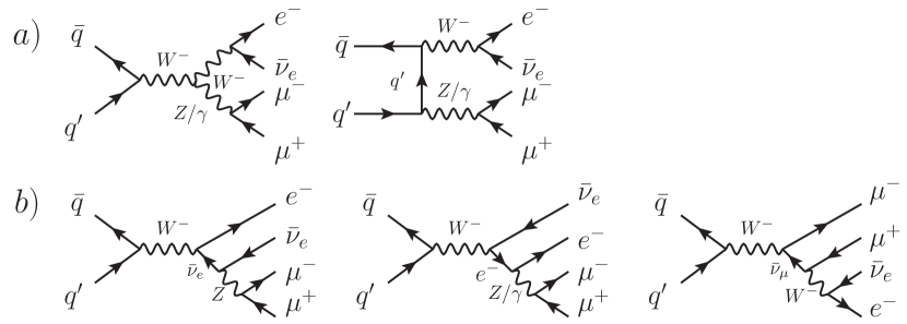
Figure 1: LO Feynman diagrams for the partonic process $\bar{q}q^{\prime}\to e^{-}\bar{\nu}_{e}\,\mu^{+}\mu^{-}$. The diagrams for the opposite-charge process $\bar{q}q^{\prime}\to e^{+}\nu_{e}\,\mu^{+}\mu^{-}$ are similar but with reversed fermion flows in the final state. a) Doubly-resonant $W^{-}Z/W^{-}\gamma$ diagrams; b) Diagrams with singly-resonant electroweak gauge bosons.

The LO hadronic differential cross section is calculated by a convolution between the partonic quark-antiquark annihilation differential cross section $d\hat{\sigma}_{\rm LO}^{\bar{q}q^{\prime}}$ and the PDFs of the first- and second-generation quarks in the proton. The PDFs, denoted $\bar{q}$ and $q^{\prime}$ below, are functions of the momentum fraction $x$ carried by the quark in the corresponding proton, and of the factorization scale $\mu_{F}$ which defines the scale at which this convolution is performed. The LO hadronic cross section reads

$$d\sigma_{\rm LO}=\int dx_{1}dx_{2}\Big{[}\bar{q}(x_{1},\mu_{F})q^{\prime}(x_{2},\mu_{F})d\hat{\sigma}_{\rm LO}^{\bar{q}q^{\prime}}+(1\leftrightarrow 2)\Big{]}.$$ (2)

In the following we will present the NLO QCD corrections and the tools that have been used for the calculation of the LO and NLO differential cross sections, and then we will focus specifically on the calculation of the EW corrections in the double-pole-approximation framework.

2.1 NLO QCD corrections

The NLO QCD corrections can be divided into the virtual corrections containing one gluon loop, and the real corrections in which one extra parton (quark, antiquark, or gluon) is included in the final state. As the final state we consider is purely leptonic, the virtual gluon can only run between the initial-state quark/antiquark pair.

The NLO QCD corrections have been calculated for on-shell production for the first time in Refs. Ohnemus:1991gb ; Frixione:1992pj , and then extended in Refs. Ohnemus:1994ff ; Dixon:1998py ; Dixon:1999di ; Campbell:1999ah ; Campbell:2011bn to include full off-shell effects and spin correlations. The NNLO QCD corrections have been calculated in Ref. Grazzini:2016swo and have been found to be of the order of an $8\%$ to $11\%$ increase of the cross section, depending on the collider energy. We limit our analysis in this paper at NLO, hence we do not include the NNLO QCD contributions in the final analysis. As the perturbative development is truncated at a fixed order, the cross section depends on the two unphysical scales $\mu_{R}$ and $\mu_{F}$, the former being the scale entering the loop functions and at which the strong coupling constant $\alpha_{s}$ is calculated, the latter being the scale at which the PDFs are evaluated and occurring in the real corrections. Our central scale choice is the natural scale of the process, $\displaystyle\mu_{R}=\mu_{F}=\mu_{0}\equiv\left(M_{W}+M_{Z}\right)/2$. The pattern of the NNLO corrections also motivate the value chosen for the central scale, as they are moderate and positive for this value of $\mu_{0}$.

We use the computer program VBFNLO 2.7.1 Arnold:2008rz ; Arnold:2011wj ; Baglio:2014uba to calculate both the LO and NLO cross sections and kinematical distributions. The implementation of the QCD corrections in this program is based on the Catani-Seymour dipole subtraction algorithm Catani:1996vz to combine the virtual and the real contributions. We will use the Hessian NNLO PDF set LUXqed17_plus_PDF4LHC15_nnlo_30 Manohar:2016nzj ; Manohar:2017eqh based on the Monte-Carlo fit PDF4LHC15 Butterworth:2015oua ; Dulat:2015mca ; Harland-Lang:2014zoa ; Ball:2014uwa ; Gao:2013bia ; Carrazza:2015aoa ; Watt:2012tq , using the QED evolution of the splitting functions described in Ref. deFlorian:2015ujt . We use the library LHAPDF 6 Buckley:2014ana and $\alpha_{s}\left(M_{Z}^{2}\right)=0.118$ as given by LUXqed17_plus_PDF4LHC15_nnlo_30. It is noted that the same PDF set is also used for LO and NLO EW results. The LO calculation has also been cross-checked against an independent calculation which is also part of the NLO EW contribution discussed in the next sub-section.

2.2 NLO EW corrections in the double-pole approximation

In the framework of the double-pole approximation, the amplitude is built using an on-shell gauge boson approximation. This is important to guarantee that the final result is gauge invariant. Therefore, Eq. (1) is now approximated as follows

$$p+p\to V_{1}(q_{1})+V_{2}(q_{2})\to\ell_{1}(k_{1})+\ell_{2}(k_{2})+\ell_{3}(k_{3})+\ell_{4}(k_{4})+X,$$ (3)

where the intermediate gauge bosons ($V_{1}=W^{\pm}$, $V_{2}=Z$) are massive and the momenta satisfy the following relations:

$$q_{1}=k_{1}+k_{2},\quad q_{2}=k_{3}+k_{4},\quad k_{i}^{2}=0,\;i=1,4,$$ (4)

At the partonic level we have

$$\bar{q}(p_{1})+q^{\prime}(p_{2})\to V_{1}(q_{1})+V_{2}(q_{2})\to\ell_{1}(k_{1})+\ell_{2}(k_{2})+\ell_{3}(k_{3})+\ell_{4}(k_{4}).$$ (5)

Since $V_{j}$ (with $j=1,2$ denoting the two gauge bosons) are on-shell, we have to map the momenta ($k_{i}$, $q_{1,2}$) to an OS momentum basis ($\hat{k}_{i}$, $\hat{q}_{1,2}$) that has the following properties

$$\hat{q}_{1}^{2} = M_{V_{1}}^{2},\quad\hat{q}_{2}^{2}=M_{V_{2}}^{2},$$

$$\hat{q}_{1} = \hat{k}_{1}+\hat{k}_{2},\quad\hat{q}_{2}=\hat{k}_{3}+\hat{k}_{4},\quad\hat{k}_{i}^{2}=0.$$ (6)

This mapping is not unique. However, it has been pointed out in Ref. Denner:2000bj that different mapping choices lead to differences of the order of $\alpha\Gamma_{V}/(\pi M_{V})$. Details of the OS mappings used in this paper are provided in Appendix A. Comparisons of different mappings are presented in Table 9 for LO cross sections and in Table 10 for NLO EW corrections.

At LO, the amplitude in the DPA is defined as (see e.g. Ref. Denner:2000bj )

$$\mathcal{A}_{\text{LO,DPA}}^{\bar{q}q^{\prime}\to V_{1}V_{2}\to 4l}=\frac{1}{Q_{1}Q_{2}}\sum_{\lambda_{1},\lambda_{2}}\mathcal{A}_{\text{LO}}^{\bar{q}q^{\prime}\to V_{1}V_{2}}\mathcal{A}_{\text{LO}}^{V_{1}\to\ell_{1}\ell_{2}}\mathcal{A}_{\text{LO}}^{V_{2}\to\ell_{3}\ell_{4}},$$ (7)

where

$$Q_{j}=q_{j}^{2}-M_{V_{j}}^{2}+iM_{V_{j}}\Gamma_{V_{j}}.$$ (8)

We note that all helicity amplitudes in the numerator are calculated with the DPA kinematics denoted by a hat. The polarization vectors in the production and decay amplitudes are physical by definition. They satisfy the following condition

$$\sum_{\lambda_{j}=1}^{3}\epsilon^{\mu}(\hat{q}_{j},\lambda_{j})\epsilon^{*\nu}(\hat{q}_{j},\lambda_{j})=-g^{\mu\nu}+\frac{\hat{q}_{j}^{\mu}\hat{q}_{j}^{\nu}}{M_{V_{j}}^{2}}.$$ (9)

It is important that the same definition is used for the polarization vectors in the production and decay amplitudes. In this way, all spin correlations are properly taken into account. It is obvious that the definition in Eq. (7) is gauge invariant because all the amplitudes on the right-hand side are individually gauge invariant. The helicity amplitudes for the production part $\mathcal{A}_{\text{LO}}^{\bar{q}q^{\prime}\to V_{1}V_{2}}$ have been calculated in our previous work Baglio:2013toa and can be taken over. For the decay amplitudes, we use the program FormCalc Hahn:1998yk ; Hahn:2000kx to generate them.

For integrated cross section, we have to take care of the two resonances of the intermediate gauge bosons, i.e. the denominator in Eq. (7). Even though it is integrable due to finite value of the widths, the phase-space integration can be more efficiently done using an appropriate mapping to smooth out the Breit-Wigner distributions. This step is also done in the VBFNLO program.

From the above definition, it becomes clear that the DPA is limited by the following factors. Not all Feynman diagrams are included, only the ones that are enhanced by two resonant weak bosons are selected, off-shell effects are missing, and the kinematics, which enter the matrix elements, are not exact. In particular, the DPA is only valid when the partonic center-of-mass energy is high enough, i.e.

$$\sqrt{\hat{s}}=\sqrt{(p_{1}+p_{2})^{2}}>M_{W}+M_{Z}.$$ (10)

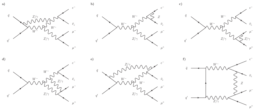
Figure 2: Representative Feynman diagrams for the NLO EW virtual corrections for the partonic process $\bar{q}q^{\prime}\to e^{-}\bar{\nu}_{e}\,\mu^{+}\mu^{-}$. Factorizable diagrams are in the top row, while non-factorizable ones in the bottom row.

We use the same principles to build the NLO EW corrections in the DPA. For this, we have to calculate the virtual and real corrections. EW corrections to both production and decay parts are separately included. However, non-factorizable corrections are neglected, since they are expected to be very small Beenakker:1997bp ; Denner:1997ia ; Denner:1998rh . The non-factorizable contribution includes all Feynman diagrams that are not parts of the on-shell $WZ$ production group or of the on-shell $V$ decay groups. These diagrams are displayed in Fig. 2, where a) belongs to the $WZ$ production group, b) the $W$ decay group, c) the $Z$ decay group, and d), e), f) the non-factorizable group. The corresponding photon-emission and quark-photon induced diagrams of the factorizable groups are fully taken into account.

The master formulas for the virtual, real-photon emission, and quark-photon induced amplitudes are schematically written as follows,

$$\delta\mathcal{A}_{\text{virt,DPA}}^{\bar{q}q^{\prime}\to V_{1}V_{2}\to 4l} =\frac{1}{Q_{1}Q_{2}}\sum_{\lambda_{1},\lambda_{2}}\left(\delta\mathcal{A}_{\text{virt}}^{\bar{q}q^{\prime}\to V_{1}V_{2}}\mathcal{A}_{\text{LO}}^{V_{1}\to\ell_{1}\ell_{2}}\mathcal{A}_{\text{LO}}^{V_{2}\to\ell_{3}\ell_{4}}\right.$$

$$\left.+\mathcal{A}_{\text{LO}}^{\bar{q}q^{\prime}\to V_{1}V_{2}}\delta\mathcal{A}_{\text{virt}}^{V_{1}\to\ell_{1}\ell_{2}}\mathcal{A}_{\text{LO}}^{V_{2}\to\ell_{3}\ell_{4}}+\mathcal{A}_{\text{LO}}^{\bar{q}q^{\prime}\to V_{1}V_{2}}\mathcal{A}_{\text{LO}}^{V_{1}\to\ell_{1}\ell_{2}}\delta\mathcal{A}_{\text{virt}}^{V_{2}\to\ell_{3}\ell_{4}}\right),$$ (11)

$$\delta\mathcal{A}_{\text{rad,DPA}}^{\bar{q}q^{\prime}\to V_{1}V_{2}\to 4l\gamma} =\sum_{\lambda_{1},\lambda_{2}}\left(\frac{\delta\mathcal{A}_{\text{rad}}^{\bar{q}q^{\prime}\to V_{1}V_{2}\gamma}\mathcal{A}_{\text{LO}}^{V_{1}\to\ell_{1}\ell_{2}}\mathcal{A}_{\text{LO}}^{V_{2}\to\ell_{3}\ell_{4}}}{Q_{1}Q_{2}}\right.$$

$$\left.+\frac{\mathcal{A}_{\text{LO}}^{\bar{q}q^{\prime}\to V_{1}V_{2}}\delta\mathcal{A}_{\text{rad}}^{V_{1}\to\ell_{1}\ell_{2}\gamma}\mathcal{A}_{\text{LO}}^{V_{2}\to\ell_{3}\ell_{4}}}{Q^{\prime}_{1}Q_{2}}+\frac{\mathcal{A}_{\text{LO}}^{\bar{q}q^{\prime}\to V_{1}V_{2}}\mathcal{A}_{\text{LO}}^{V_{1}\to\ell_{1}\ell_{2}}\delta\mathcal{A}_{\text{rad}}^{V_{2}\to\ell_{3}\ell_{4}\gamma}}{Q_{1}Q^{\prime}_{2}}\right),$$ (12)

$$\delta\mathcal{A}_{\text{ind,DPA}}^{q\gamma\to V_{1}V_{2}\to 4lq^{\prime}} =\sum_{\lambda_{1},\lambda_{2}}\frac{\delta\mathcal{A}_{\text{ind}}^{q\gamma\to V_{1}V_{2}q^{\prime}}\mathcal{A}_{\text{LO}}^{V_{1}\to\ell_{1}\ell_{2}}\mathcal{A}_{\text{LO}}^{V_{2}\to\ell_{3}\ell_{4}}}{Q_{1}Q_{2}},$$ (13)

where the correction amplitudes $\delta\mathcal{A}_{\text{virt}}^{\bar{q}q^{\prime}\to V_{1}V_{2}}$, $\delta\mathcal{A}_{\text{rad}}^{\bar{q}q^{\prime}\to V_{1}V_{2}\gamma}$, and $\delta\mathcal{A}_{\text{ind}}^{q\gamma\to V_{1}V_{2}q^{\prime}}$ have been calculated in the OS production calculation in Ref. Baglio:2013toa and are reused here. The missing pieces related to the corrections to the decay amplitudes are generated again by FormCalc and combined together using the dipole-subtraction method Catani:1996vz ; Dittmaier:1999mb ; Basso:2015gca . The new variables $Q^{\prime}_{1}$ and $Q^{\prime}_{2}$ are defined as in Eq. (8) but with the gauge-boson momenta being reconstructed from the $1\to 3$ decays. For the cross-section contributions, we have

$$\Delta\sigma_{\text{virt,DPA}}^{\bar{q}q^{\prime}\to V_{1}V_{2}\to 4l} \propto 2\text{Re}\left[\delta\mathcal{A}_{\text{virt,DPA}}^{\bar{q}q^{\prime}\to V_{1}V_{2}\to 4l}\mathcal{A}_{\text{LO,DPA}}^{\bar{q}q^{\prime}\to V_{1}V_{2}\to 4l\star}\right],$$ (14)

$$\Delta\sigma_{\text{rad,DPA}}^{\bar{q}q^{\prime}\to V_{1}V_{2}\to 4l\gamma} \propto|\delta\mathcal{A}_{\text{rad,DPA}}^{\bar{q}q^{\prime}\to V_{1}V_{2}\to 4l\gamma}|^{2}\;\;\text{with interference terms neglected},$$ (15)

$$\Delta\sigma_{\text{ind,DPA}}^{q\gamma\to V_{1}V_{2}\to 4lq^{\prime}} \propto|\delta\mathcal{A}_{\text{ind,DPA}}^{q\gamma\to V_{1}V_{2}\to 4lq^{\prime}}|^{2}.$$ (16)

For later use, the following corrections coming from the radiative decays are defined.

$$\Delta\sigma^{\text{virt}}_{\text{d}V_{1}} \propto 2\text{Re}\left[\left(\sum_{\lambda_{1},\lambda_{2}}\frac{\mathcal{A}_{\text{LO}}^{\bar{q}q^{\prime}\to V_{1}V_{2}}\delta\mathcal{A}_{\text{virt}}^{V_{1}\to\ell_{1}\ell_{2}}\mathcal{A}_{\text{LO}}^{V_{2}\to\ell_{3}\ell_{4}}}{Q_{1}Q_{2}}\right)\mathcal{A}_{\text{LO,DPA}}^{\bar{q}q^{\prime}\to V_{1}V_{2}\to 4l\star}\right],$$ (17)

$$\Delta\sigma^{\text{rad}}_{\text{d}V_{1}} \propto|\sum_{\lambda_{1},\lambda_{2}}\frac{\mathcal{A}_{\text{LO}}^{\bar{q}q^{\prime}\to V_{1}V_{2}}\delta\mathcal{A}_{\text{rad}}^{V_{1}\to\ell_{1}\ell_{2}\gamma}\mathcal{A}_{\text{LO}}^{V_{2}\to\ell_{3}\ell_{4}}}{Q^{\prime}_{1}Q_{2}}|^{2},$$ (18)

$$\Delta\sigma^{\text{virt}}_{\text{d}V_{2}} \propto 2\text{Re}\left[\left(\sum_{\lambda_{1},\lambda_{2}}\frac{\mathcal{A}_{\text{LO}}^{\bar{q}q^{\prime}\to V_{1}V_{2}}\mathcal{A}_{\text{LO}}^{V_{1}\to\ell_{1}\ell_{2}}\delta\mathcal{A}_{\text{virt}}^{V_{2}\to\ell_{3}\ell_{4}}}{Q_{1}Q_{2}}\right)\mathcal{A}_{\text{LO,DPA}}^{\bar{q}q^{\prime}\to V_{1}V_{2}\to 4l\star}\right],$$ (19)

$$\Delta\sigma^{\text{rad}}_{\text{d}V_{2}} \propto|\sum_{\lambda_{1},\lambda_{2}}\frac{\mathcal{A}_{\text{LO}}^{\bar{q}q^{\prime}\to V_{1}V_{2}}\mathcal{A}_{\text{LO}}^{V_{1}\to\ell_{1}\ell_{2}}\delta\mathcal{A}_{\text{rad}}^{V_{2}\to\ell_{3}\ell_{4}\gamma}}{Q_{1}Q^{\prime}_{2}}|^{2}.$$ (20)

Further technical details on how the momenta and the amplitudes are calculated are provided in Appendix A.

From the above terms we define schematically some important EW corrections to understand various effects as follows

$$\delta_{\bar{q}q^{\prime}} =\left(\Delta\sigma_{\text{virt,DPA}}^{\bar{q}q^{\prime}\to V_{1}V_{2}\to 4l}+\Delta\sigma_{\text{rad,DPA}}^{\bar{q}q^{\prime}\to V_{1}V_{2}\to 4l\gamma}\right)/\sigma_{\text{LO}},$$ (21)

$$\delta_{q\gamma} =\Delta\sigma_{\text{ind,DPA}}^{q\gamma\to V_{1}V_{2}\to 4lq^{\prime}}/\sigma_{\text{LO}},$$ (22)

$$\delta_{\text{NLOEW}} =\delta_{\bar{q}q^{\prime}}+\delta_{q\gamma},$$ (23)

$$\delta_{\text{d}V_{1}} =(\Delta\sigma^{\text{virt}}_{\text{d}V_{1}}+\Delta\sigma^{\text{rad}}_{\text{d}V_{1}})/\sigma_{\text{LO}},$$ (24)

$$\delta_{\text{p}V_{1}} =\delta_{\text{NLOEW}}-\delta_{\text{d}V_{1}},$$ (25)

and $\delta_{\text{d}V_{2}}$, $\delta_{\text{p}V_{2}}$ for the second gauge boson are similarly defined. $\delta_{q\gamma}$ is interesting because it is sensitive to the photon PDF and can be large. This correction is also provided in Ref. Biedermann:2017oae , so that a numerical comparison will be later performed. $\delta_{\text{d}V_{j}}$ (total correction to $V_{j}$ decay) and $\delta_{\text{p}V_{j}}$ (total correction to $V_{j}$ production) are interesting for polarization observables of the $V_{j}$ boson as mentioned in the introduction. These effects will be presented in Table 2 and in Appendix D.

In the calculation of polarization observables, the LO results must be always included. By default, our NLO EW results are the sum of the full LO results and the EW corrections calculated in the DPA. In addition, if not explicitly mentioned, NLO means NLO QCD and EW.

2.3 Definition of fiducial polarization observables

At LO in the DPA, the angular distribution of a final-state lepton created by an on-shell massive gauge boson is described as

$$\frac{d\sigma}{\sigma d\!\cos\theta d\phi} =\frac{3}{16\pi}\Big{[}(1+\cos^{2}\theta)+A_{0}\frac{1}{2}(1-3\cos^{2}\theta)+A_{1}\sin(2\theta)\cos\phi$$

$$+A_{2}\frac{1}{2}\sin^{2}\theta\cos(2\phi)+A_{3}\sin\theta\cos\phi+A_{4}\cos\theta$$

$$+A_{5}\sin^{2}\theta\sin(2\phi)+A_{6}\sin(2\theta)\sin\phi+A_{7}\sin\theta\sin\phi\Big{]},$$ (26)

where $A_{0-7}$ are dimensionless angular coefficients, $\theta$ and $\phi$ are the lepton polar and azimuthal angles, respectively, in the rest frame of the massive gauge boson in a particular coordinate system that needs to be specified. In the case of the charged lepton coming from the $W$ decay, we set the notation $\theta=\theta_{3}$, $\phi=\phi_{3}$. For the negatively charged lepton coming from the $Z$ decay, we set $\theta=\theta_{6}$, $\phi=\phi_{6}$. We note that the rest frame of the $W$ bosons cannot be reconstructed in experiments as the longitudinal momentum of the neutrino is unknown. However, this can be calculated if the on-shell condition $(p_{e}+p_{\nu_{e}})^{2}=M_{W}^{2}$ is imposed and then choosing the solution with smaller magnitude ATLAS:2018ogj . This step is not done in the present paper but should be done if comparisons with measurements are performed.

It is important to note that Eq. (26) is only correct if there is no restriction on the phase space of the individual leptons. We will use the term polarization observables to refer to the coefficients $A_{i}$ or the polarization fractions below defined.

Polarizations of the gauge bosons can be described using a spin-density matrix. In the DPA and at LO, for the process at hand, this matrix reads

$$\rho^{V_{j}}_{\lambda\lambda^{\prime}}=C\sum_{s_{q},s_{l}}\mathcal{A}_{\bar{q}q^{\prime}\to l_{i}l^{\prime}_{i}V_{j}}^{*}(\lambda,s_{q},s_{l})\mathcal{A}_{\bar{q}q^{\prime}\to l_{i}l^{\prime}_{i}V_{j}}(\lambda^{\prime},s_{q},s_{l}),$$ (27)

where $s_{q}$ and $s_{l}$ denote the set of quark and lepton helicities, respectively and $C$ is a normalization factor determined from the condition $\text{Tr}(\rho^{V_{j}})=1$. Since $\rho^{V_{j}}$ is Hermitian, the spin-density matrix is parameterized by eight coefficients, equivalent to the definition by Eq. (26). It is noted that the matrix $\rho^{V_{j}}$ is independent of the decay $V_{j}\to l_{j}l^{\prime}_{j}$. However, when we calculate the angular coefficients by using Eq. (26) at NLO EW, they receive contributions from EW corrections to the decays. These effects are therefore interesting and deserve special attention.

At LO in the EW coupling and for a single $V$ resonance, direct relations between the angular coefficients and the elements of the spin-density matrix of the gauge boson can be proved as shown in Refs. Aguilar-Saavedra:2015yza ; Ballestrero:2017bxn for the $W$ boson and in Ref. Aguilar-Saavedra:2017zkn for the $Z$ boson. This is the reason why the angular coefficients are also called spin or polarization observables. We give here the explicit relations between the angular coefficients and the spin-density matrix elements $\rho_{ij}$ with $i,j=+,0,-$, that can be directly read off from the results of Refs. Aguilar-Saavedra:2015yza ; Aguilar-Saavedra:2017zkn ,

$$A_{0} =2\rho_{00},\;A_{1}=\frac{1}{\sqrt{2}}(\rho_{+0}-\rho_{-0}+\rho_{0+}-\rho_{0-}),$$

$$A_{2} =2(\rho_{+-}+\rho_{-+}),\;A_{3}=\sqrt{2}b(\rho_{+0}+\rho_{-0}+\rho_{0+}+\rho_{0-}),$$

$$A_{4} =2b(\rho_{++}-\rho_{--}),\;A_{5}=\frac{1}{i}(\rho_{-+}-\rho_{+-}),$$

$$A_{6} =-\frac{1}{i\sqrt{2}}(\rho_{+0}+\rho_{-0}-\rho_{0+}-\rho_{0-}),\;A_{7}=\frac{\sqrt{2}b}{i}(\rho_{0+}-\rho_{0-}-\rho_{+0}+\rho_{-0}),$$ (28)

where $b=1$ for the $W^{\pm}$ bosons and $b=-c$ for the $Z$ boson, with

$$c=\frac{g_{L}^{2}-g_{R}^{2}}{g_{L}^{2}+g_{R}^{2}}=\frac{1-4s^{2}_{W}}{1-4s^{2}_{W}+8s^{4}_{W}},\quad s^{2}_{W}=1-\frac{M_{W}^{2}}{M_{Z}^{2}}.$$ (29)

Numerically, we have $c\approx 0.21$. Since $A_{i}$ are real, we see that $A_{5}$, $A_{6}$, $A_{7}$ come from the imaginary part of the spin-density matrix elements.

We can also calculate the three coefficients $f_{L}$, $f_{R}$, and $f_{0}$, called fiducial polarization fractions and defined as (see e.g. Bern:2011ie ; Stirling:2012zt )

$$\frac{d\sigma}{\sigma d\!\cos\theta_{3}} \equiv\frac{3}{8}\Big{[}(1\mp\cos\theta_{3})^{2}f^{W^{\pm}}_{L}+(1\pm\cos\theta_{3})^{2}f^{W^{\pm}}_{R}+2\sin^{2}\theta_{3}f^{W^{\pm}}_{0}\Big{]},$$

$$\frac{d\sigma}{\sigma d\!\cos\theta_{6}} \equiv\frac{3}{8}\Big{[}(1+\cos^{2}\theta_{6}+2c\cos\theta_{6})f^{Z}_{L}+(1+\cos^{2}\theta_{6}-2c\cos\theta_{6})f^{Z}_{R}+2\sin^{2}\theta_{6}f^{Z}_{0}\Big{]},$$ (30)

where the upper signs are for $W^{+}$ and the lower signs are for $W^{-}$, $c$ defined in Eq. (29) ocurring because the $Z$ boson decays into both left- and right-handed muons.

To see the relations between the polarization fractions and angular coefficients, we perform the integration over $\phi\in[0,2\pi]$ of Eq. (26). We obtain

$$\frac{d\sigma}{\sigma d\!\cos\theta}=\frac{3}{8}\Big{[}(1+\cos^{2}\theta)+A_{0}\frac{1}{2}(1-3\cos^{2}\theta)+A_{4}\cos\theta\Big{]}.$$ (31)

Defining the expectation of observables $f(\theta)$ and $g(\theta,\phi)$ as

$$\langle f(\theta)\rangle =\int_{-1}^{1}d\!\cos\theta f(\theta)\frac{1}{\sigma}\frac{d\sigma}{d\!\cos\theta},$$ (32)

$$\langle g(\theta,\phi)\rangle =\int_{-1}^{1}d\!\cos\theta\int_{0}^{2\pi}d\phi g(\theta,\phi)\frac{d\sigma}{\sigma d\!\cos\theta d\phi},$$ (33)

which can be calculated from $\cos\theta$ and $\cos\theta$-$\phi$ distributions, we have

$$A_{0} =4-\langle 10\cos^{2}\theta\rangle,\;A_{1}=\langle 5\sin 2\theta\cos\phi\rangle,\;A_{2}=\langle 10\sin^{2}\theta\cos 2\phi\rangle,\;A_{3}=\langle 4\sin\theta\cos\phi\rangle,$$

$$\;A_{4} =\langle 4\cos\theta\rangle,\;A_{5}=\langle 5\sin^{2}\theta\sin 2\phi\rangle,\;A_{6}=\langle 5\sin 2\theta\sin\phi\rangle,\;A_{7}=\langle 4\sin\theta\sin\phi\rangle,$$ (34)

which agree with Ref. Bern:2011ie . We then obtain (see also Ref. Bern:2011ie for the $W^{\pm}$ bosons and Ref. Stirling:2012zt for the $Z$ boson),

$$f^{W^{\pm}}_{L} =-\frac{1}{2}\mp\langle\cos\theta_{3}\rangle+\frac{5}{2}\langle\cos^{2}\theta_{3}\rangle,\;f^{W^{\pm}}_{R}=-\frac{1}{2}\pm\langle\cos\theta_{3}\rangle+\frac{5}{2}\langle\cos^{2}\theta_{3}\rangle,$$

$$f^{W^{\pm}}_{0} =2-5\langle\cos^{2}\theta_{3}\rangle,$$ (35)

$$f^{Z}_{L} =-\frac{1}{2}+\frac{1}{c}\langle\cos\theta_{6}\rangle+\frac{5}{2}\langle\cos^{2}\theta_{6}\rangle,\;f^{Z}_{R}=-\frac{1}{2}-\frac{1}{c}\langle\cos\theta_{6}\rangle+\frac{5}{2}\langle\cos^{2}\theta_{6}\rangle,$$

$$f^{Z}_{0} =2-5\langle\cos^{2}\theta_{6}\rangle,$$ (36)

which satisfy $f_{L}+f_{R}+f_{0}=1$. The relations between the polarization fractions and angular coefficients read

$$f^{W^{\pm}}_{L} =\frac{1}{4}(2-A^{W^{\pm}}_{0}\mp A^{W^{\pm}}_{4}),\;\;f^{W^{\pm}}_{R}=\frac{1}{4}(2-A^{W^{\pm}}_{0}\pm A^{W^{\pm}}_{4}),\;\;f^{W^{\pm}}_{0}=\frac{1}{2}A^{W^{\pm}}_{0},$$

$$f^{Z}_{L} =\frac{1}{4}(2-A^{Z}_{0}+\frac{1}{c}A^{Z}_{4}),\;\;f^{Z}_{R}=\frac{1}{4}(2-A^{Z}_{0}-\frac{1}{c}A^{Z}_{4}),\;\;f^{Z}_{0}=\frac{1}{2}A^{Z}_{0}.$$ (37)

In the present work, we will go beyond the DPA and beyond LO. Realistic cuts on the individual lepton momenta as used by ATLAS or CMS are also required. The eight angular coefficients are therefore no longer enough to describe the angular distributions Stirling:2012zt ; Ballestrero:2017bxn . However, the equations from (32) to (37) can still be used. The coefficients $A_{i}$ are now defined as the projections of realistic angular distributions calculated with full matrix elements at any order in perturbation theory and with arbitrary cuts on the individual leptons. This definition has been used and discussed in Ref. Stirling:2012zt .

To distinguish with the usual polarization observables used for the case of full lepton phase space such as in $W+\text{jets}$ production Bern:2011ie , we will refer to those as inclusive polarization observables. When cuts on the individual lepton momenta are used, we call them fiducial polarization observables or fiducial angular coefficients. When moving from the full phase space to fiducial phase space, the cuts on $p_{T,\ell}$ and $\eta_{\ell}$ reduce event fraction at $|\cos\theta_{\ell,V}|\approx 1$. Therefore, the fiducial longitudinal fractions $f_{0}^{V}$ are larger than the corresponding inclusive fractions.

The effects of EW corrections on the gauge-boson decays for the fiducial polarization coefficients will be shown in Appendix D, where effects from EW corrections to the production process $\bar{q}q^{\prime}\to l_{i}l^{\prime}_{i}V_{j}$ are also presented. In this appendix, one can also compare the full LO to the DPA LO results to see the off-shell effects, which are not present in the DPA approximation.

It is important to note that $\sigma$ in Eq. (26) and Eq. (30) can be replaced by a differential distribution such as Stirling:2012zt

$$\sigma\to\frac{d\sigma}{dp_{T,V}},\;\frac{d\sigma}{dp_{T,\ell}},\;\ldots.$$ (38)

From the $\cos\theta$-$p_{T,V}$ distribution we can calculate $d\sigma_{L,R,0}/dp_{T,V}$. In this paper, we will show fiducial polarization results for $p_{T,W}$, $p_{T,Z}$, $\eta_{Z}$ (pseudo-rapidity), and $y_{Z}$ (rapidity) distributions as the corresponding results for the inclusive polarization fractions exist, while it is not the case for the individual lepton momentum distributions. Results for $d\sigma/dp_{T,\ell}$ and for $d\sigma/dy_{\ell}$ in $W+\text{jets}$ production have been presented in Ref. Stirling:2012zt . We however do not discuss them in this work.

We now address the issue of choosing a coordinate system. In this work, we will consider and compare two coordinate systems:

• Helicity (HE) coordinate system: This coordinate system is defined in Ref. Bern:2011ie , where the $z^{\prime}$-axis (the prime is used to denote the gauge-boson rest frame) is along the momentum of the gauge boson in the laboratory frame ($p_{V}$). The exact definitions of $x^{\prime}$ and $y^{\prime}$ axes are given in Ref. Bern:2011ie and a representation of the HE coordinate system is depicted in Fig. 3 (left).

• Collins-Soper (CS) coordinate system: This coordinate system was defined in Ref. Collins:1977iv . We use in our paper the convention followed by Ref. Karlberg:2014qua ; Aad:2016izn . The $z^{\prime}$-axis is defined as follows. Let $P_{1}=(E,0,0,+E)$ and $P_{2}=(E,0,0,-E)$ are the momenta of the two protons in the laboratory frame. Then $P^{\prime}_{1}$ and $P^{\prime}_{2}$ are the corresponding momenta in the gauge boson rest frame. The $z^{\prime}$-axis is the bisector of $\vec{P}_{1}$ and $-\vec{P}_{2}$. Furthermore, the $z^{\prime}$-axis points into the hemisphere of $p_{V}$. The $x^{\prime}-z^{\prime}$ plane is the plane of $P^{\prime}_{1}$ and $P^{\prime}_{2}$. The $x^{\prime}$-axis is perpendicular to the $z^{\prime}$-axis and points into the hemisphere of $-(\vec{P^{\prime}}_{1}+\vec{P^{\prime}}_{2})$. The coordinate system is right-handed, which defines the $y^{\prime}$-axis. A representation of the CS coordinate system is depicted in Fig. 3 (right).

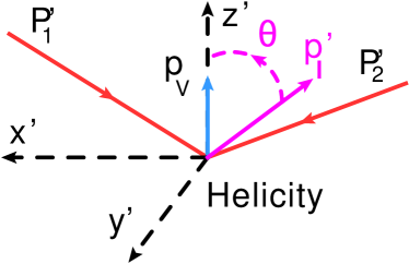
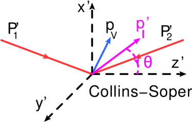
Figure 3: Representation of the HE coordinate systems (left) and the CS coordinate systems (right), in the rest frame of the vector boson $V$ under consideration. The corresponding angle $\theta$ for the charged lepton is also defined.

3 Numerical setup and theoretical uncertainties

In this section we specify our input parameters, which are used to obtain numerical results presented in Section 4, Section 5, and Appendix D. Our best results at NLO QCD+EW are calculated using the full NLO QCD matrix elements combined with the NLO EW corrections calculated using the DPA.

3.1 Input parameters and definition of kinematical cuts

The input parameters are

$$G_{\mu}=1.16637\times 10^{-5}{\,\text{GeV}}^{-2},\,M_{W}=80.385{\,\text{GeV}},\,M_{Z}=91.1876{\,\text{GeV}},$$

$$\Gamma_{W}=2.085{\,\text{GeV}},\,\Gamma_{Z}=2.4952{\,\text{GeV}},\,M_{t}=173{\,\text{GeV}},\,M_{H}=125{\,\text{GeV}},$$ (39)

essentially based on Ref. Agashe:2014kda and are the same as the ones used in Ref. Baglio:2013toa . The masses of the leptons and the light quarks, i.e. all but the top mass, are approximated as zero. This is justified because our results are insensitive to those small masses. The electromagnetic coupling is calculated as $\alpha_{G_{\mu}}=\sqrt{2}G_{\mu}M_{W}^{2}(1-M_{W}^{2}/M_{Z}^{2})/\pi$.

We will give results for the LHC running at a center-of-mass energy $\sqrt{s}=13\,{\,\text{TeV}}$. We will consider ATLAS and CMS cuts for their corresponding fiducial phase space, both for $e^{+}\nu_{e}\,\mu^{+}\mu^{-}$ and $e^{-}\bar{\nu}_{e}\,\mu^{+}\mu^{-}$ final states. We treat the extra parton occurring in the NLO QCD corrections inclusively and we do not apply any jet cuts. We also consider the possibility of lepton-photon recombination, where we redefine the momentum of a given charged lepton $\ell$ as being $p^{\prime}_{\ell}=p_{\ell}+p_{\gamma}$ if $\Delta R(\ell,\gamma)\equiv\sqrt{(\Delta\eta)^{2}+(\Delta\phi)^{2}}<0.1$ for ATLAS and CMS cuts. This recombination is done before applying the following kinematical cuts related to the charged leptons. For ATLAS we also define this transverse mass,

$$m_{T,W}\equiv\sqrt{2p_{T,\nu}p_{T,e}[1-\cos\Delta\phi(e,\nu)]},$$ (40)

where $\Delta\phi(e,\nu)$ is the angle between the electron and the neutrino in the transverse plane Aaboud:2016yus . The sets of cuts are identical for $e^{+}\nu_{e}\,\mu^{+}\mu^{-}$ and $e^{-}\bar{\nu}_{e}\,\mu^{+}\mu^{-}$ final states. We use $\ell$ for either $e$ or $\mu$.

The cuts for ATLAS at $13\,{\,\text{TeV}}$ are given in Ref. Aaboud:2016yus . The CMS cuts for $13\,{\,\text{TeV}}$ are given in Ref. Khachatryan:2016tgp . The complete list of the cuts we have used for our analysis is summarized in Table 1.

ATLAS fiducial	CMS fiducial
$\begin{matrix}p_{T,\mu}>15{\,\text{GeV}},\quad p_{T,e}>20{\,\text{GeV}},\quad|\eta_{\ell}|<2.5,\\ \Delta R\left(e,\mu^{\pm}\right)>0.3,\quad\Delta R\left(\mu^{+},\mu^{-}\right)>0.2,\\ \left|m_{\mu^{+}\mu^{-}}-M_{Z}\right|<10{\,\text{GeV}},\quad m_{T,W}>30{\,\text{GeV}}\end{matrix}$	$\begin{matrix}p^{\text{leading}}_{T,\mu}>20{\,\text{GeV}},\quad p^{\text{sub-leading}}_{T,\mu}>10{\,\text{GeV}},\\ p_{T,e}>20{\,\text{GeV}},\quad|\eta_{\ell}|<2.5,\\ \quad 60{\,\text{GeV}}<m_{\mu^{+}\mu^{-}}<120{\,\text{GeV}}\end{matrix}$

Table 1: List of the cuts used in our fiducial-phase-space analysis at the 13 TeV LHC, depending on the experiment under consideration. They are extracted from Refs. Aaboud:2016yus ; Khachatryan:2016tgp .

3.2 Theoretical uncertainties

We consider two sources of theoretical uncertainties in this work. The first uncertainty we consider comes from the truncation of the perturbative expansion at a given order. This truncation leads to a dependence of the cross section on two unphysical scales, the renormalization scale $\mu_{R}$ and the factorization scale $\mu_{F}$. We evaluate the scale uncertainties by varying independently these two scales as $n\mu_{0}/2$ with $n=1,2,4$ and $\mu_{0}=(M_{W}+M_{Z})/2$ being our central scale choice. We further use the constraint $1/2\leq\mu_{R}/\mu_{F}\leq 2$ to limit the number of scale choices to seven at NLO QCD. It is noted that $\mu_{R}$ does not appear at LO and hence there are only three possibilities for choosing $\mu_{F}$.

The second uncertainty we consider is due to the uncertainties in the determination of the PDFs. We use the 30 Hessian error sets provided by LUXqed17_plus_PDF4LHC15_nnlo to calculate the PDF uncertainty as Butterworth:2015oua

$$\Delta^{\rm PDF}\sigma=\sqrt{\sum_{i=1}^{30}\left(\sigma_{i}-\sigma_{0}\right)^{2}},$$ (41)

where $\sigma_{i}$ stands for the calculation using the $i$th error set and $\sigma_{0}$ stands for the calculation using the central set. Note that Eq. (41) will also be used for the calculation of the PDF uncertainty affecting the polarization observables and their associated kinematical distributions presented in Section 5.

In the numerical results, we will present also the NLO QCD+EW predictions calculated with the central PDF set and with the central scale $\mu_{0}$. The PDF and scale uncertainties are calculated using the NLO QCD results. This is acceptable as long as the EW corrections are small. In the ideal case, the EW corrections should also be calculated for all members of the PDF set and for all scale choices, and then the NLO QCD+EW errors would be computed from there. This is more important for the polarization observables as the combination of QCD and EW corrections is not a linear summation, see the discussion in Section 5.1. This step is however not done in the present work as it requires a lot of computing power, since the calculation of the EW corrections is much more complicated than the QCD one. Besides, the information we would get when performing such a full analysis is expected not to be substantially different from our current analysis, given the size of the uncertainties (see Section 5 and Appendix C).

In the following the PDF errors are indicated in round brackets, statistical errors in square brackets, and the scale errors being asymmetric are indicated using upper and lower superscripts, unless otherwise stated.

It is noted that the calculation of the statistical error for polarization observables defined by Eq. (32) and Eq. (33) are nontrivial as the correlations between different bins are unknown. As a simple exercise, one can try to calculate the total cross section and its statistical error from a two-dimensional distribution, say the LO $\cos\theta^{\text{HE}}_{e}$ distribution shown in Fig. 13, and compare them with the known results in Table 2. One will see that there is agreement for the central value but not for the error. If we sum the errors of all the bins linearly, it overshoots the true value (that is the one given in the table) by a factor of $4$. If summation in quadrature is used, then it undershoots by a factor of $1/2$. Moreover, for three-dimensional distributions, the statistical error for each bin is not known in many Monte-Carlo programs including the VBFNLO code. And it gets worse when higher-order corrections are included, because the calculation of the statistical error for every bin becomes more difficult and therefore unreliable.

Fortunately, in the framework of Monte-Carlo method, there is a simple way to get an estimate for the statistical errors for any observables independently of the complexity of the calculation, that is to use different random-number seeds to get a list of central values. From this list the mean value and an estimate for the statistical error are obtained as follows

$$\bar{\sigma}=\frac{1}{N}\sum_{i=1}^{N}\sigma_{i},\quad\Delta\sigma=\frac{1}{\sqrt{N-1}}\sqrt{\sum_{i=1}^{N}(\sigma_{i}-\bar{\sigma})^{2}},$$ (42)

where $N$ is the number of random seeds. Using this method for the $\cos\theta^{\text{HE}}_{e}$ distribution above mentioned, we get the LO cross section, for the $e^{+}\nu_{e}\mu^{+}\mu^{-}$ final state with the ATLAS fiducial cuts, $19.345\pm 0.003{\,\text{fb}}$ with $N=10$, which is in good agreement with the value of $19.344\pm 0.002{\,\text{fb}}$ obtained by using the standard Monte-Carlo integration method with one random seed. This method also helps to smooth out statistical fluctuations, thereby giving nicer plots for distributions. All numerical results for kinematical distributions and polarization observables presented in this paper are obtained using this method with $N=50$ $(10)$ for the NLO QCD (EW) results. For polarization observables, there are actually two ways to do the seed average. One method is to do the seed average for all relevant distributions to get the seed-combined distributions first. Then from these combined distributions we proceed to calculate polarization observables. The second method is to calculate the polarization observables for every seed first, then combine these observables using Eq. (42). We have checked that both methods give the same central values, but the second way provides also the statistical errors.

Finally, we remark that the statistical errors are very small compared to the PDF and scale uncertainties. They will be therefore not indicated, unless where necessary.

4 Results for fiducial cross sections and kinematical distributions

We present in this section our results for the cross section in the fiducial phase space, including scale and parton distribution function (PDF) uncertainties, as well as a selection of kinematical distributions. Our results are presented in such a way that direct comparisons between the full calculation of Ref. Biedermann:2017oae and our DPA for the NLO EW corrections are possible. For this comparison, it is noted that the input parameter scheme of Ref. Biedermann:2017oae is different from ours as follows. Ref. Biedermann:2017oae uses the complex mass scheme, which introduces a shift in $s_{W}^{2}$ and other parameters due to the widths of the $W$ and $Z$ bosons. They used a non-diagonal CKM matrix, taking into account the effect of the Cabibbo mixing angle. Lastly, they used the first version of LUXqed_plus_PDF4LHC15_nnlo_100 for PDF set, while we use the latest version. The difference on the photon PDF is very minor Manohar:2017eqh , and since both versions use PDF4LHC15_nnlo the differences on the quark and gluon PDFs should be also negligible. These effects on the fiducial cross sections are quantified at the end of Section 4.1. The total difference is small, of about $1\%$ for the ATLAS fiducial cross sections at full LO.

4.1 Fiducial cross sections

We start this subsection by presenting a comparison of our results for the cross sections with the experimental measurements from ATLAS and CMS. It is important to note that our predictions are not the state-of-the-art as we are not including the NNLO QCD corrections that would amount to $\simeq+10\%$ Grazzini:2017ckn . Nevertheless we wish to do an NLO comparison to confirm that we do use the same setup as ATLAS and CMS.

The latest ATLAS results, obtained with 36 fb^-1 of data, allow for a comparison channel by channel. In Table 4 of Ref. ATLAS:2018ogj we find the following results,

$$\sigma_{e^{+}\mu^{+}\mu^{-}}^{\rm ATLASfid}=36.7\pm 2.5\,\,\mathrm{fb},\quad\sigma_{e^{-}\mu^{+}\mu^{-}}^{\rm ATLASfid}=25.7\pm 2.1\,\,\mathrm{fb},$$ (43)

to be compared to our NLO QCD+EW results,

$$\sigma_{e^{+}\mu^{+}\mu^{-}}^{\rm th,ATLASfid}=34.7\pm 0.5\,({\rm PDF})+1.8/\!-1.5\,({\rm scale})-0.8\,({\rm NLOEW})\,\,\mathrm{fb},$$

$$\sigma_{e^{-}\mu^{+}\mu^{-}}^{\rm th,ATLASfid}=24.1\pm 0.4\,({\rm PDF})+1.3/\!-1.1\,({\rm scale})-0.6\,({\rm NLOEW})\,\,\mathrm{fb}.$$ (44)

Comparing Eq. (43) and Eq. (44) we get about $1\sigma$ agreement between ATLAS experimental results and our theoretical predictions at NLO.

The latest CMS results we get in the literature have been obtained with 2.3 fb^-1 of data and collect together $W^{+}$ and $W^{-}$ channels as well as all leptonic decay modes Khachatryan:2016tgp , reading

$$\sigma_{W^{\pm}Z}^{\rm CMSfid}=258\pm 30\,\,\mathrm{fb}.$$ (45)

Our NLO QCD+EW predictions for the leptonic channel $e^{\pm}\nu_{e}\,\mu^{+}\mu^{-}$ read

$$\sigma_{e^{+}\mu^{+}\mu^{-}}^{\rm th,CMSfid}=44.7\pm 0.7\,({\rm PDF})+2.4/\!-1.9\,({\rm scale})-0.5\,({\rm NLOEW})\,\,\mathrm{fb},$$

$$\sigma_{e^{-}\mu^{+}\mu^{-}}^{\rm th,CMSfid}=30.7\pm 0.5\,({\rm PDF})+1.7/\!-1.4\,({\rm scale})-0.3\,({\rm NLOEW})\,\,\mathrm{fb}.$$ (46)

We can combine the results in Eq. (46) by assuming the same cross-section for the four different leptonic modes $e^{\pm}\mu^{+}\mu^{-}$, $\mu^{\pm}e^{+}e^{-}$, $e^{\pm}e^{+}e^{-}$, $\mu^{\pm}\mu^{+}\mu^{-}$, and adding our predictions for $W^{+}$ and $W^{-}$ channels. Adding the uncertainties in quadrature, we finally obtain at NLO QCD+EW

$$\sigma_{W^{\pm}Z}^{\rm th,CMSfid}=302\pm 2\,({\rm PDF})+6/\!-5\,({\rm scale})-3\,({\rm NLOEW})\,\mathrm{fb}.$$ (47)

We compare our prediction in Eq. (47) with the experimental result in Eq. (45) and obtain a $1.3\sigma$ agreement at NLO.

Cut	Process	LO [fb]	DPA LO [fb]	$\delta_{\bar{q}q^{\prime}}$(%)	$\delta_{q\gamma}$(%)	$\delta_{\text{d}W}$(%)	$\delta_{\text{d}Z}$(%)	$\delta_{\text{NLOEW}}$(%)
ATLAS fid.	$e^{+}\nu_{e}\mu^{+}\mu^{-}$	$19.344[2]$	$18.740[2]$	$-6.10$	$+1.76$	$-1.20$	$-3.55$	$-4.34$
ATLAS fid.	$e^{-}\bar{\nu}_{e}\mu^{+}\mu^{-}$	$13.001[1]$	$12.987[1]$	$-6.11$	$+1.86$	$-1.15$	$-3.55$	$-4.25$
CMS fid.	$e^{+}\nu_{e}\mu^{+}\mu^{-}$	$24.6225[4]$	$23.510[2]$	$-3.63$	$+1.77$	$-1.09$	$-1.19$	$-1.86$
CMS fid.	$e^{-}\bar{\nu}_{e}\mu^{+}\mu^{-}$	$16.3205[2]$	$16.157[1]$	$-3.62$	$+1.90$	$-1.05$	$-1.16$	$-1.72$

Table 2: Born cross sections in fb obtained using the full and DPA matrix elements with the ATLAS and CMS fiducial cuts. The EW corrections in percentage calculated using DPA normalized to the LO are also shown.

To shed light on the goodness of the DPA and to compare with the full results of Ref. Biedermann:2017oae , we present in Table 2 the LO, DPA LO, and the NLO EW corrections calculated using DPA relative to the LO results with the ATLAS and CMS fiducial cuts. The definitions of the corrections $\delta_{\bar{q}q^{\prime}}$ and $\delta_{q\gamma}$ are the same as those in Ref. Biedermann:2017oae and are given in Eq. (49). We observe that the DPA cross sections are smaller than the full results, with the difference about $-3\,(-5)\%$ for the $W^{+}Z$ channel with the ATLAS (CMS) fiducial cuts. For the $W^{-}Z$ case, the differences are much smaller. The corrections to the decays of the $W$ and $Z$ bosons, defined in Section 2.2, are also separately shown. These are new compared to our previous results for OS production Baglio:2013toa .

Before commenting on the differences between our results and those of Ref. Biedermann:2017oae , it is important to know the effects of the differences in the input parameter schemes as above mentioned. We have checked at the full LO with the ATLAS fiducial cuts that setting the Cabibbo angle to zero as in this work increases the cross section about $0.7\,(0.9)\%$ compared to the case of $\sin\theta_{\text{c}}=0.225$ as used in Ref. Biedermann:2017oae for the $W^{+}Z$ ($W^{-}Z$) channels. We have also implemented the complex-mass scheme of Ref. Biedermann:2017oae , i.e. taking into account the shifts in $M_{V}$, $\Gamma_{V}$ (with $V=W,Z$), $\alpha_{G_{\mu}}$, $s^{2}_{W}$ due to $\Gamma_{V}^{\text{os}}$ as in their Section 3.1, and obtained that this effect is about $0.2\%$ for both channels, with the complex-mass scheme cross sections being smaller. The differences due to different versions of the PDF set are completely negligible as expected. Overall, the differences in the input parameters between Ref. Biedermann:2017oae and this work are about $1\%$ for both channels, which are essentially the sum of those two effects.

Comparing to the results of Ref. Biedermann:2017oae for the ATLAS fiducial cuts, we see good agreement for $\delta_{q\gamma}$ and $\delta_{\bar{q}q^{\prime}}$ individually. As seen in the following Section 4.2, similar agreement is also obtained for several kinematical distributions. Comparisons between the DPA with non-factorizable corrections included and the full results for the case of $pp\to W^{+}W^{-}\to\nu_{\mu}\mu^{+}e^{-}\bar{\nu}_{e}+X$ and of $e^{+}e^{-}\to W^{+}W^{-}\to$ 4 fermions have been presented in Ref. Biedermann:2016guo and Ref. Denner:2005es , respectively. Good agreement has also been observed there.

4.2 Kinematical distributions: $W^{+}Z$ channel

In order to get more insight into the theoretical uncertainties affecting the process we study a selection of differential distributions including the scale and PDF uncertainties at NLO QCD. We limit our discussion to the $W^{+}Z$ channel and present the corresponding plots for the $W^{-}Z$ channel in Appendix B. We first start with the transverse momentum distributions of the $e^{+}\nu_{e}$ and $\mu^{+}\mu^{-}$ systems and we display in Fig. 4 the predictions using the ATLAS fiducial cuts and in Fig. 10 the predictions using the CMS fiducial cuts. The transverse momentum distribution of the neutrino and rapidity distribution of the $\mu^{+}\mu^{-}$ system are also shown in those figures (bottom row). In both cases we also display the total theoretical uncertainty calculated as a linear sum of PDF and scale uncertainties at NLO QCD, shown as bands around the central prediction calculated at $\mu_{F}=\mu_{R}=(M_{W}+M_{Z})/2$. We follow the recommendations of Ref. Dittmaier:2011ti to combine PDF and scale uncertainties linearly. This procedure was also implemented in Ref. Aad:2016ett by ATLAS. Cross sections at NLO QCD+EW are also displayed in blue, and the LO predictions in green, in the top panels.

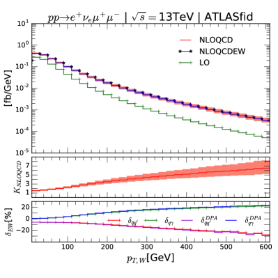
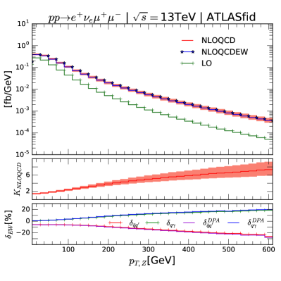
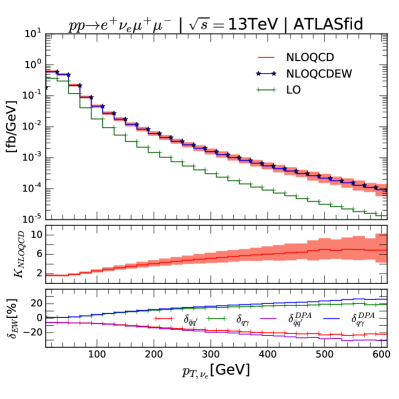
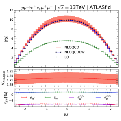
Figure 4: Distributions of the transverse momentum of the $e^{+}\nu_{e}$ (top left) and $\mu^{+}\mu^{-}$ (top right) systems and of the neutrino (bottom left) in the processes $pp\to e^{+}\nu_{e}\,\mu^{+}\mu^{-}+X$ at the 13 TeV LHC with the ATLAS fiducial cuts. Rapidity distribution of the $\mu^{+}\mu^{-}$ system is also displayed at the bottom right corner. The upper panels show the absolute values of the cross sections at LO (in green), NLO QCD (red), and NLO QCD+EW (blue). The middle panels display the ratio of the NLO QCD cross sections to the corresponding LO ones. The bands indicate the total theoretical uncertainty calculated as a linear sum of PDF and scale uncertainties at NLO QCD. The bottom panels show the NLO EW corrections (see text) calculated using DPA relative to the full LO (marked with plus signs) and DPA LO cross sections.

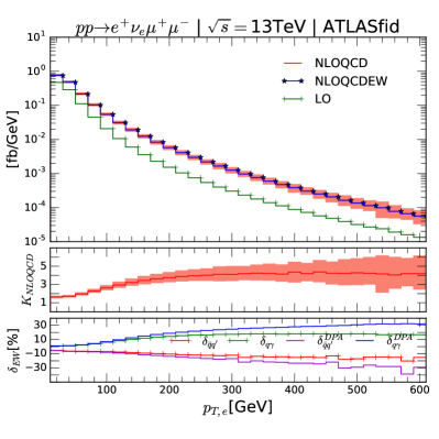
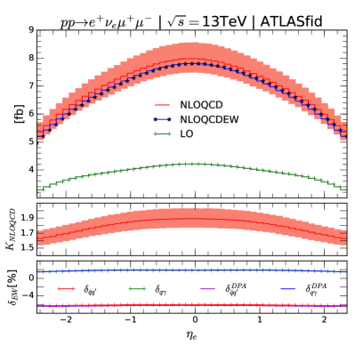
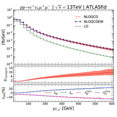
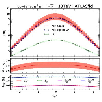
Figure 5: Same as Fig. 4 but for the transverse momentum and pseudo-rapidity distributions of the positron (top row) and the muon (bottom row).

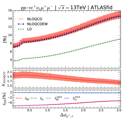
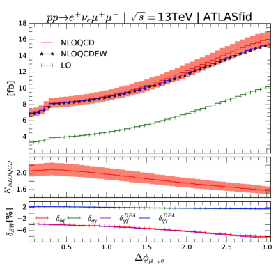
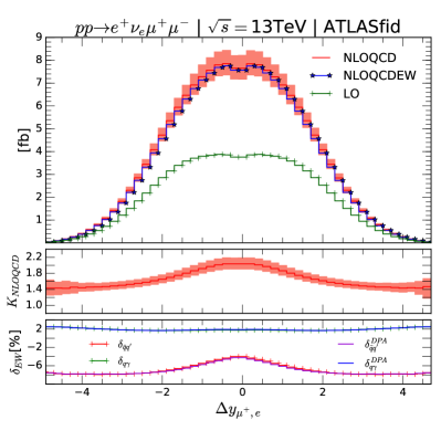
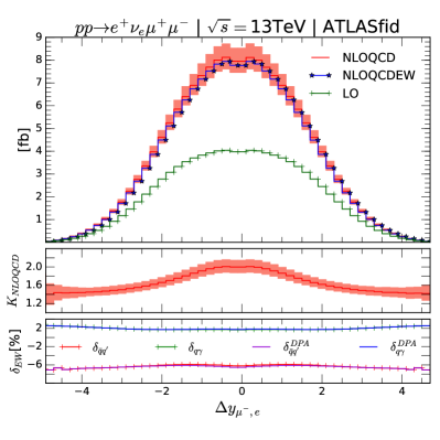
Figure 6: Same as Fig. 4 but for the azimuthal-angle difference (top row) and the rapidity difference (bottom row) between the $\mu^{+}$ and $e^{+}$ (left column) and between the $\mu^{-}$ and $e^{+}$ (right column).

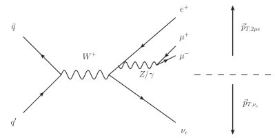
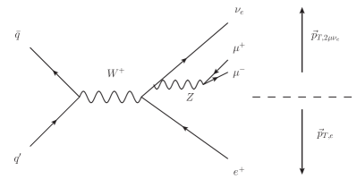
Figure 7: Illustration of the diagrammatic structures non present in the DPA and that dominate the $p_{T,e}$ distribution (left) and the $p_{T,\nu}$ distribution (right), for high transverse momentum.

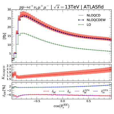
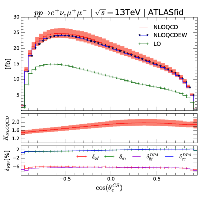
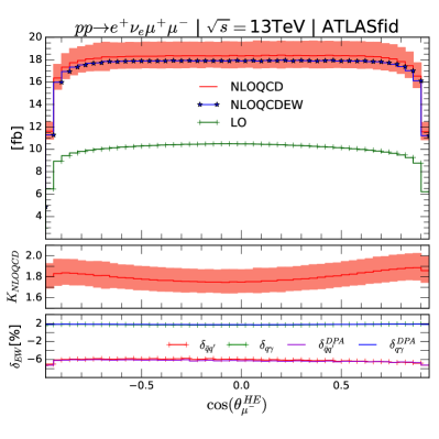
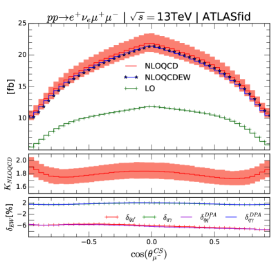
Figure 8: Same as Fig. 4 but for the $\cos\theta$ distributions of the electron (top row) calculated in the Helicity (left) and Collins-Soper (right) coordinate systems. The same distributions for the muon are shown in the bottom row.

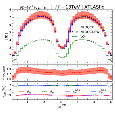
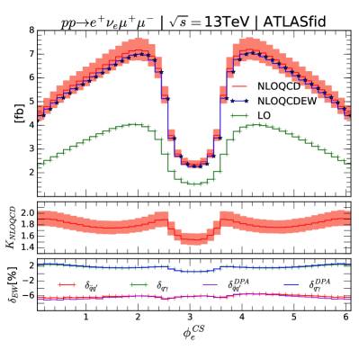
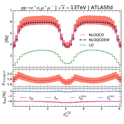
Figure 9: Same as Fig. 4 but for the azimuthal-angle distributions of the electron (top row) calculated in the Helicity (left) and Collins-Soper (right) coordinate systems. The same distributions for the muon are shown in the bottom row.

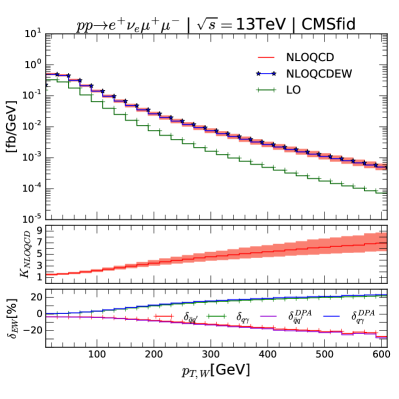
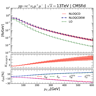
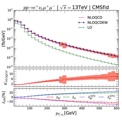
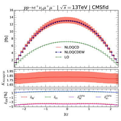
Figure 10: Same as Fig. 4 but with the CMS fiducial cuts.

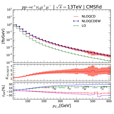
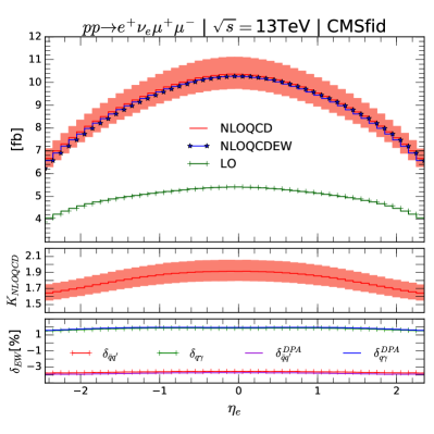
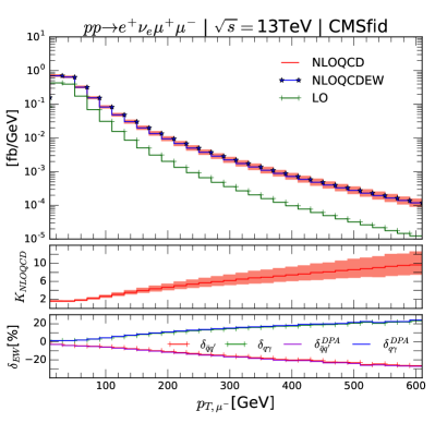
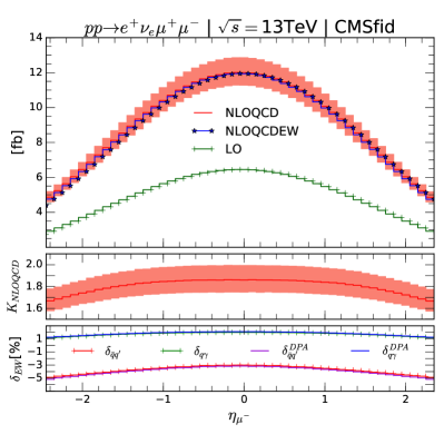
Figure 11: Same as Fig. 5 but with the CMS fiducial cuts.

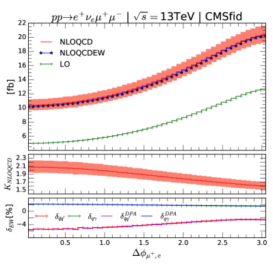
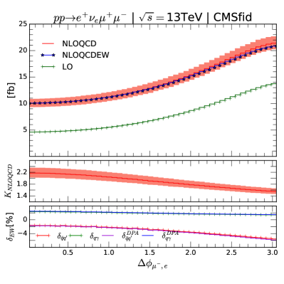
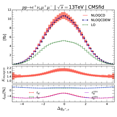
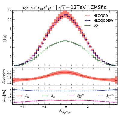
Figure 12: Same as Fig. 6 but with the CMS fiducial cuts.

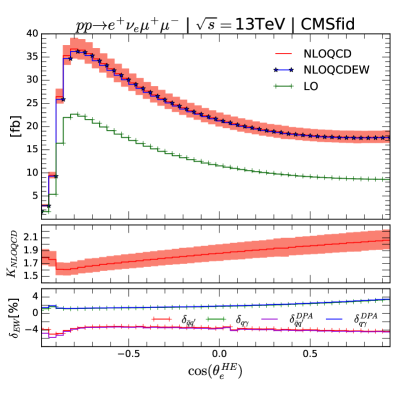
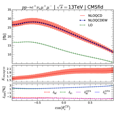
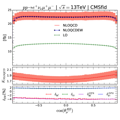
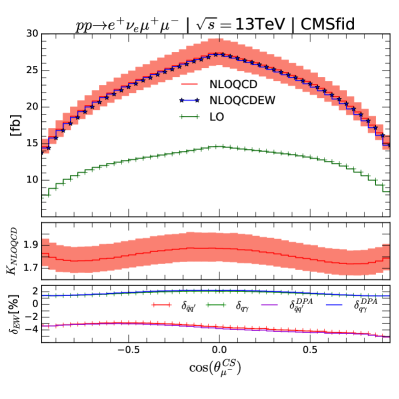
Figure 13: Same as Fig. 8 but with the CMS fiducial cuts.

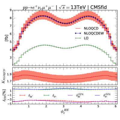
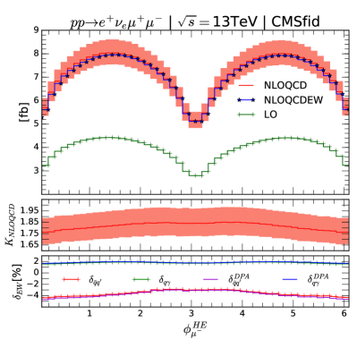
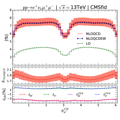
Figure 14: Same as Fig. 9 but with the CMS fiducial cuts.

In the middle panels we display the $K$-factor defined as

$$K_{\text{NLOQCD}}=\frac{d\sigma_{\text{NLOQCD}}}{d\sigma_{\text{LO}}}.$$ (48)

Please note that we use the same NNLO PDF set in the numerator and the denominator. In the bottom panels we show the NLO EW corrections calculated using DPA as explained in Section 2.2 relative to the full and DPA Born cross sections. These corrections are defined as

$$\delta_{\bar{q}q^{\prime}} =\frac{d\Delta\sigma^{\text{NLOEW}}_{\bar{q}q^{\prime}}}{d\sigma^{\text{LO}}},\quad\delta_{q\gamma}=\frac{d\Delta\sigma^{\text{NLOEW}}_{q\gamma}}{d\sigma^{\text{LO}}},$$

$$\delta_{\bar{q}q^{\prime}}^{\text{DPA}} =\frac{d\Delta\sigma^{\text{NLOEW}}_{\bar{q}q^{\prime}}}{d\sigma^{\text{LO}}_{\text{DPA}}},\quad\delta_{q\gamma}^{\text{DPA}}=\frac{d\Delta\sigma^{\text{NLOEW}}_{q\gamma}}{d\sigma^{\text{LO}}_{\text{DPA}}}.$$ (49)

The total NLO EW correction is the sum of $\delta_{\bar{q}q^{\prime}}$ and $\delta_{q\gamma}$. Those EW corrections are defined in the same way as in Ref. Biedermann:2017oae , thereby enabling direct comparisons of our DPA NLO EW corrections to the full results.

As already observed in OS production Baglio:2013toa , the $K$-factors in the $p_{T}$ distributions are increasing over the $p_{T}$ range to reach high values at high transverse momentum because of soft weak boson emission in the quark-gluon and quark-photon induced processes. For example, it reaches $K_{\text{NLOQCD}}=6.5$ at $p_{T,W}=600$ GeV and $K_{\text{NLOQCD}}\simeq 8$ at $p_{T,Z}=600$ GeV. The same observation is true for the transverse momentum distributions of the individual final-state leptons displayed in Fig. 4 and Fig. 5. The uncertainties are also increasing from close to $\pm 5\%$ at low $p_{T}$ up to $\simeq\pm 40\%$ at high $p_{T}$. Similar distributions can be obtained with the CMS fiducial cuts, as displayed in Fig. 10 and Fig. 11. In that case, the $K$ factors are a bit smaller and the uncertainties are also smaller, reaching $\simeq\pm 20\%$ at high $p_{T}$, closer to the uncertainties that can be obtained in the OS production.

The EW corrections are nearly identical when using DPA or full LO matrix elements for the transverse momenta of the $e^{+}\nu_{e}$ and $\mu^{+}\mu^{-}$ systems, as well as for the individual muons. The Sudakov regime of the $\bar{q}q^{\prime}$ contribution is cancelled by the quark-photon induced contributions that reach $+20\%$ at $p_{T,W/Z}=600$ GeV. The distributions of the individual final-state leptons of the $W$ boson system, however, display differences between the DPA and the full LO matrix elements. This can be traced back to the contribution of a $Z$ radiated off the electron or the neutrino and splitting into the di-muon pair. This contribution, displayed in Fig. 7, does not exist in the DPA and can lead to a higher $p_{T,e/\nu}$ due to the hard $\mu^{+}\mu^{-}$ system that needs to be balanced by the transverse momentum of the electron or the neutrino. The EW corrections calculated with the full LO matrix elements should then be smaller in magnitude than the corresponding EW corrections with the DPA matrix elements, as observed in Fig. 4 (lower left) and Fig. 5 (upper left). The same is true for the CMS fiducial cuts as displayed in Fig. 10 (lower left) and Fig. 11 (upper left). Similar differences between the DPA and the full results for the case of $pp\to W^{+}W^{-}\to\nu_{\mu}\mu^{+}e^{-}\bar{\nu}_{e}+X$ have been discussed in Ref. Biedermann:2016guo .

The $Z$ boson rapidity distribution displayed in Fig. 4 (lower right) as well as the pseudo-rapidity distributions of the charged leptons displayed in Fig. 5 (right-hand side) show non-constant $K$-factors of order 2 and EW corrections close to $-4\%$, summing the quark-photon induced contributions and the $\bar{q}q^{\prime}$ contributions.

The theoretical uncertainties at NLO are limited to $\simeq\pm 5\%$. We remind that the $\simeq+10\%$ correction stemming from the NNLO QCD corrections Grazzini:2017ckn is not included there.

Similar distributions are also obtained for the CMS fiducial cuts displayed in Fig. 10 (lower right) and Fig. 11 (right-hand side).

We also display azimuthal-angle difference distributions in Fig. 6 (ATLAS fiducial cuts) and Fig. 12 (CMS fiducial cuts), that can be directly compared to Ref. Biedermann:2017oae . Other distributions including $p_{T,Z}$, $p_{T,\nu_{e}}$, $p_{T,e}$, $y_{Z}$, $\eta_{\ell}$, $\ldots$, can be compared as well. Comparing our kinematical distributions to those of Ref. Biedermann:2017oae , we observe good agreement in shape and magnitude for $\delta_{\bar{q}q^{\prime}}$ and $\delta_{q\gamma}$ corrections individually.

For completeness, we also display the $\cos\theta$ and $\phi$ distributions in Fig. 8 and Fig. 9 respectively, for ATLAS fiducial cuts. The corresponding distributions for the CMS fiducial cuts are given in Fig. 13 and Fig. 14. The Helicity coordinate system is displayed on the left-hand side while the Collins-Soper coordinate system is displayed on the right-hand side, in all plots. The $K$-factors are not constant and the theoretical uncertainties are quite limited, ranging from $\simeq\pm 5\%$ to $\simeq\pm 20\%$. In all distributions, the DPA and the full LO matrix elements give the same EW corrections.

5 Numerical results for fiducial polarization observables: $W^{+}Z$ channel

5.1 Fiducial angular coefficients and polarization fractions: $W^{+}Z$ channel

We start the discussion of the fiducial polarization observables with a presentation of the NLO QCD and EW predictions for the angular coefficients and the polarization fractions including PDF and scale uncertainties. We will also display the LO results to get an insight into the size of the NLO corrections. We calculate the polarization coefficients via the numerical integration of the $\cos\theta-\phi$ distributions while the polarization fractions are calculated via the numerical integration of $\cos\theta$ distributions. The statistical uncertainty in the case of the NLO QCD predictions is found to be negligible compared to the PDF or scale uncertainty and is not given. We use the bin-averaging method for the numerical integration, that gives for $n\times n$ bins $[a_{i},b_{i}]\times[c_{j},d_{j}]$,

$$\left\langle f(\theta)\right\rangle =\int_{-1}^{1}d\!\cos\theta f(\theta)\frac{d\sigma}{\sigma d\!\cos\theta}\simeq\frac{1}{\sigma}\sum_{i=1}^{n}\left(\frac{d\sigma}{d\!\cos\theta}\right)_{i}f_{i},$$ (50)

$$\left\langle g(\theta,\phi)\right\rangle =\int_{-1}^{1}d\!\cos\theta\int_{0}^{2\pi}d\phi g(\theta,\phi)\frac{d\sigma}{\sigma d\!\cos\theta d\phi}\simeq\frac{1}{\sigma}\sum_{1\leq i,j\leq n}\left(\frac{d\sigma}{d\!\cos\theta d\phi}\right)_{ij}g_{ij},$$ (51)

with

$$f_{i}=\frac{1}{b_{i}-a_{i}}\int_{a_{i}}^{b_{i}}f(\theta)d\!\cos\theta,\quad g_{ij}=\frac{1}{\left(b_{i}-a_{i}\right)\left(d_{j}-c_{j}\right)}\int_{a_{i}}^{b_{i}}d\!\cos\theta\int_{c_{j}}^{d_{j}}d\phi g(\theta,\phi),$$ (52)

where the integrals in Eq. (52) are analytically performed.

Another obvious choice to calculate $f_{i}$ and $g_{ij}$ reads, for each bin,

$$f_{i}=f(\theta_{i}),\quad g_{ij}=g(\theta_{i},\phi_{i}),$$ (53)

where $\theta_{i}$ and $\phi_{i}$ correspond to the middle of the bin. We have checked that results obtained from both methods are in good agreement. In the following, all numerical results are calculated using the bin-averaging method.

The results for the fiducial coefficients $A_{0-7}$, depending on the choice of the coordinate system (either HE or CS as defined in Section 2.3), obtained using the full NLO QCD matrix elements and the EW corrections in the DPA, are presented in Table 3 (for the $W$ boson) and Table 4 (for the $Z$ boson) for the process $pp\to e^{+}\nu_{e}\,\mu^{+}\mu^{-}+X$ using the ATLAS fiducial cuts. The corresponding results using the CMS fiducial cuts are given in Table 5 and Table 6. The QCD corrections are always sizable in all coordinate systems, while the EW corrections are more limited. As already seen in $W^{+}+j$ production at the LHC Bern:2011ie , the inclusive coefficients $A_{5}$, $A_{6}$, and $A_{7}$ are very small even after taking into account the QCD corrections. The higher-order corrections can sometimes switch the sign of these coefficients, see e.g. $A_{7}^{e^{+}}$ in the HE coordinate system. The smallness of these coefficients can be understood from the DPA LO results provided in Appendix D, where we can see that they are all consistently zero within the statistical errors, independent of the cuts or the coordinate system. This is also in line with the fact that those coefficients are, at the DPA LO and in the inclusive

phase-space limit, proportional to the imaginary parts of the spin-density matrix elements as shown in Eq. (28), therefore expected to be vanishing. The scale and PDF uncertainties are very small, at maximum a few percents, as expected from an observable built over a ratio of cross sections.

Method	$A_{0}$	$A_{1}$	$A_{2}$	$A_{3}$	$A_{4}$	$A_{5}$	$A_{6}$	$A_{7}$
HE LO	$1.026(2)^{+5}_{-6}$	$-0.286(2)^{+4}_{-3}$	$-1.314(2)^{+3}_{-3}$	$-0.251(2)^{+2}_{-2}$	$-0.447(7)^{+3}_{-3}$	$-0.002(0.2)^{+0.03}_{-0}$	$-0.001(0.3)^{+0.1}_{-0.1}$	$-0.004(0.2)^{+0.1}_{-0.02}$
HE NLOEW	$1.028$	$-0.284$	$-1.324$	$-0.252$	$-0.438$	$-0.004$	$-0.004$	$0.003$
HE NLOQCD	$1.016(1)^{+3}_{-4}$	$-0.326(2)^{+2}_{-3}$	$-1.413(2)^{+10}_{-12}$	$-0.229(1)^{+2}_{-1}$	$-0.295(7)^{+11}_{-11}$	$-0.001(1)^{+0.1}_{-0.2}$	$-0.0002(6)^{+3}_{-2}$	$0.003(1)^{+1}_{-0.5}$
HE NLOQCDEW	$1.017$	$-0.326$	$-1.420$	$-0.229$	$-0.287$	$-0.002$	$-0.002$	$0.007$
CS LO	$1.397(3)^{+4}_{-5}$	$0.229(1)^{+3}_{-3}$	$-0.945(1)^{+2}_{-2}$	$0.003(2)^{+0.3}_{-1}$	$-0.613(8)^{+4}_{-4}$	$-0.0002(3)^{+0.1}_{-1}$	$0.002(0.3)^{+0.1}_{-0.04}$	$0.004(0.2)^{+0.01}_{-0.1}$
CS NLOEW	$1.402$	$0.225$	$-0.952$	$0.008$	$-0.608$	$0.001$	$0.006$	$-0.003$
CS NLOQCD	$1.513(3)^{+7}_{-7}$	$0.192(1)^{+2}_{-2}$	$-0.918(3)^{+2}_{-2}$	$0.061(4)^{+4}_{-4}$	$-0.469(6)^{+10}_{-10}$	$-0.0001(11)^{+0}_{-3}$	$0.001(0.5)^{+0.3}_{-0.2}$	$-0.003(0.4)^{+1}_{-1}$
CS NLOQCDEW	$1.518$	$0.189$	$-0.921$	$0.065$	$-0.463$	$0.0004$	$0.003$	$-0.007$

Table 3: Fiducial angular coefficients of the $e^{+}$ distribution for the process $pp\to e^{+}\nu_{e}\,\mu^{+}\mu^{-}+X$ at LO, NLO EW, NLO QCD and NLO QCD+EW at the 13 TeV LHC with the ATLAS fiducial cuts. Results are presented for two coordinate systems: the helicity (HE) and Collins-Soper (CS) coordinate systems. The PDF uncertainties (in parenthesis) and the scale uncertainties are provided for the LO and NLO QCD results, all given on the last digit of the central prediction.

Method	$A_{0}$	$A_{1}$	$A_{2}$	$A_{3}$	$A_{4}$	$A_{5}$	$A_{6}$	$A_{7}$
HE LO	$1.035(2)^{+2}_{-2}$	$-0.304(1)^{+2}_{-1}$	$-0.705(1)^{+0.3}_{-1}$	$0.063(1)^{+0.04}_{-0.1}$	$-0.017(1)^{+1}_{-1}$	$-0.007(0.4)^{+0.1}_{-0}$	$-0.007(0.2)^{+0}_{-0.2}$	$0.003(0.2)^{+0}_{-0.1}$
HE NLOEW	$1.039$	$-0.307$	$-0.717$	$0.050$	$-0.020$	$-0.007$	$-0.008$	$0.003$
HE NLOQCD	$0.985(2)^{+5}_{-6}$	$-0.306(1)^{+4}_{-3}$	$-0.734(1)^{+2}_{-2}$	$0.031(1)^{+2}_{-2}$	$0.003(1)^{+1}_{-1}$	$-0.004(1)^{+0.3}_{-0.4}$	$-0.004(1)^{+0.3}_{-0.2}$	$0.003(1)^{+0.2}_{-0}$
HE NLOQCDEW	$0.986$	$-0.308$	$-0.742$	$0.023$	$0.001$	$-0.004$	$-0.004$	$0.003$
CS LO	$1.254(2)^{+2}_{-3}$	$0.239(2)^{+2}_{-2}$	$-0.488(1)^{+1}_{-1}$	$-0.061(0.3)^{+0.3}_{-0.4}$	$0.035(1)^{+1}_{-1}$	$-0.0001(3)^{+1}_{-0}$	$0.010(0.3)^{+0.1}_{-0.004}$	$-0.003(0.2)^{+0.1}_{-0}$
CS NLOEW	$1.266$	$0.234$	$-0.493$	$-0.053$	$0.023$	$0.001$	$0.012$	$-0.003$
CS NLOQCD	$1.267(2)^{+4}_{-4}$	$0.221(1)^{+1}_{-1}$	$-0.455(2)^{+2}_{-2}$	$-0.021(1)^{+3}_{-3}$	$0.023(1)^{+1}_{-1}$	$0.0004(6)^{+2}_{-2}$	$0.006(0.5)^{+0.2}_{-0.4}$	$-0.003(1)^{+0}_{-0.1}$
CS NLOQCDEW	$1.273$	$0.218$	$-0.457$	$-0.016$	$0.016$	$0.001$	$0.007$	$-0.003$

Table 4: Same as Table 3 but for the $\mu^{-}$ distribution.

Method	$A_{0}$	$A_{1}$	$A_{2}$	$A_{3}$	$A_{4}$	$A_{5}$	$A_{6}$	$A_{7}$
HE LO	$0.897(2)^{+5}_{-6}$	$0.088(3)^{+6}_{-5}$	$-0.626(2)^{+4}_{-3}$	$-0.373(3)^{+3}_{-4}$	$-0.488(8)^{+3}_{-4}$	$-0.002(0.3)^{+0.1}_{-0}$	$-0.001(0.3)^{+0.04}_{-0}$	$-0.003(0.3)^{+0}_{-0.05}$
HE NLOEW	$0.899$	$0.092$	$-0.625$	$-0.374$	$-0.480$	$-0.004$	$-0.004$	$0.003$
HE NLOQCD	$0.913(1)^{+2}_{-3}$	$0.023(2)^{+4}_{-4}$	$-0.672(1)^{+3}_{-3}$	$-0.321(2)^{+3}_{-3}$	$-0.325(7)^{+12}_{-11}$	$-0.001(1)^{+0.2}_{-0.2}$	$-0.0003(5)^{+3}_{-2}$	$0.003(0.5)^{+0.5}_{-1}$
HE NLOQCDEW	$0.915$	$0.025$	$-0.672$	$-0.321$	$-0.319$	$-0.002$	$-0.002$	$0.006$
CS LO	$0.760(4)^{+8}_{-9}$	$0.196(1)^{+3}_{-3}$	$-0.764(1)^{+1}_{-1}$	$0.052(2)^{+0.4}_{-1}$	$-0.723(9)^{+4}_{-6}$	$-0.00003(28)^{+2}_{-1}$	$0.002(0.4)^{+0}_{-0.1}$	$0.003(0.3)^{+0.05}_{-0}$
CS NLOEW	$0.758$	$0.192$	$-0.767$	$0.057$	$-0.719$	$0.001$	$0.006$	$-0.003$
CS NLOQCD	$0.875(3)^{+7}_{-6}$	$0.172(1)^{+1}_{-2}$	$-0.711(3)^{+4}_{-4}$	$0.097(4)^{+3}_{-3}$	$-0.551(7)^{+12}_{-11}$	$-0.0002(6)^{+1}_{-1}$	$0.001(1)^{+0.2}_{-0.2}$	$-0.003(0.5)^{+1}_{-0.5}$
CS NLOQCDEW	$0.875$	$0.170$	$-0.712$	$0.100$	$-0.547$	$0.0002$	$0.003$	$-0.007$

Table 5: Same as Table 3 but with the CMS fiducial cuts.

Method	$A_{0}$	$A_{1}$	$A_{2}$	$A_{3}$	$A_{4}$	$A_{5}$	$A_{6}$	$A_{7}$
HE LO	$0.858(3)^{+3}_{-4}$	$-0.273(1)^{+1}_{-1}$	$-0.570(1)^{+0.5}_{-1}$	$0.068(1)^{+0.1}_{-0}$	$-0.022(1)^{+1}_{-1}$	$-0.007(0.2)^{+0.1}_{-0}$	$-0.006(0.2)^{+0.1}_{-0.1}$	$0.003(0.2)^{+0.1}_{-0.02}$
HE NLOEW	$0.855$	$-0.282$	$-0.574$	$0.055$	$-0.026$	$-0.007$	$-0.008$	$0.002$
HE NLOQCD	$0.785(2)^{+8}_{-9}$	$-0.300(1)^{+3}_{-2}$	$-0.592(2)^{+1}_{-1}$	$0.033(1)^{+2}_{-3}$	$0.001(1)^{+2}_{-2}$	$-0.004(1)^{+0.2}_{-0.2}$	$-0.004(1)^{+0.2}_{-0.2}$	$0.003(1)^{+0.02}_{-0.2}$
HE NLOQCDEW	$0.782$	$-0.304$	$-0.594$	$0.026$	$-0.001$	$-0.004$	$-0.004$	$0.003$
CS LO	$1.128(2)^{+1}_{-1}$	$0.296(2)^{+2}_{-2}$	$-0.303(1)^{+2}_{-1}$	$-0.069(0.5)^{+0.4}_{-1}$	$0.038(2)^{+1}_{-1}$	$-0.0003(2)^{+1}_{-0}$	$0.010(0.4)^{+0}_{-0.1}$	$-0.003(0.2)^{+0.02}_{-0.1}$
CS NLOEW	$1.141$	$0.291$	$-0.290$	$-0.062$	$0.025$	$0.0005$	$0.012$	$-0.002$
CS NLOQCD	$1.180(2)^{+3}_{-3}$	$0.275(1)^{+1}_{-1}$	$-0.200(3)^{+7}_{-8}$	$-0.024(1)^{+3}_{-3}$	$0.024(1)^{+1}_{-1}$	$0.0003(5)^{+1}_{-1}$	$0.006(0.5)^{+0.3}_{-0.3}$	$-0.003(1)^{+0.2}_{-0.01}$
CS NLOQCDEW	$1.188$	$0.272$	$-0.192$	$-0.019$	$0.017$	$0.001$	$0.006$	$-0.003$

Table 6: Same as Table 4 but with the CMS fiducial cuts.

The results for the fiducial polarization fractions $f_{L}$, $f_{R}$, and $f_{0}$ are given in Table 7 for the case of the ATLAS fiducial cuts, while the results for the CMS fiducial cuts are displayed in Table 8. It is noted that these fractions can be also calculated from the angular coefficients provided in Table 3 and Table 4. The results of the ATLAS and CMS fiducial cuts are similar in the HE coordinate system, except that the L and R fractions are higher with the CMS fiducial cuts than with the ATLAS fiducial cuts. In the CS coordinate system, however, there is a sizable difference for $f_{R}^{W^{+}}$, that is close to zero and negative at LO for the ATLAS fiducial cuts while being positive and of the order of $0.13$ for the CMS fiducial cuts. We note that having a negative fraction is possible when looking at Eq. (30). This happens because we are considering fiducial fractions and are using the Collins-Soper coordinate system. The fiducial fractions are all positive in the helicity system. This can be understood because the $z$ axis is aligned along the vector-boson direction of flight in the helicity system, but not in the Collins-Soper one. In the limit of LO DPA and of inclusive cut, the polarization fractions in the helicity system can be proven to be positive because they are truly fractions.

The QCD corrections are sizable in all polarization fractions. The EW corrections, however, are negligible for the $W^{+}$ polarization fractions and small but noticeable for the $Z$ polarization fraction, in particular reaching $+4\%$ ($-5\%$) of the NLO QCD results for the $f_{R}^{Z}$ ($f_{L}^{Z}$) fractions in the $W^{+}Z$ channel in the CS coordinate system with either the ATLAS or CMS fiducial cuts, see Table 7 and Table 8. The EW corrections are a bit higher, reaching $+7\%$ ($-4\%$) for the $f_{R}^{Z}$ ($f_{L}^{Z}$) fractions in the $W^{-}Z$ channel in the HE coordinate system with the ATLAS fiducial cuts, see Table 15.

We trace back the origin of the large EW correction to the $f_{R}^{Z}$ fraction to the angular coefficient $A_{4}$. We see that the EW correction to the $A_{4}^{Z}$ in the $W^{+}Z$ channel in the CS coordinate system with the ATLAS fiducial cuts is $-30\%$ compared to the NLO QCD prediction, see Table 4. This can be further understood by inspecting Table 18 in Appendix D, where we observe two things: (i) The $q\gamma$ correction is negligible, while the $\bar{q}q^{\prime}$ one is large. (ii) The origin of this large EW correction comes from the radiative decay of the $Z$ boson. The EW correction to the $Z$ decay, including both the virtual and real photon emission contributions, induces $-36\%$ correction to the DPA LO result. It would be interesting to see if these large effects are still present when considering the inclusive polarization observables $A_{i}$, because, as discussed in Section 2.3, the spin-density matrix defined in Eq. (27) is independent of the decay mode. Similar large EW corrections are also seen in the coefficient $A_{3}^{Z}$, where it is also due to the radiative corrections to the $Z$ decay.

It is worth noting that $A_{3}^{Z}$ and $A_{4}^{Z}$ are proportional to the EW parameter $c$, which is very sensitive to the value of $s^{2}_{W}$, see Eq. (28), while it is not the case for the $W$ bosons. So, it may be not so surprising after all that they are sensitive to the EW corrections to the $Z$ decay.

The PDF uncertainty is very limited, of the order of $\pm 1\%$ at maximum, and the scale uncertainty is also very small, of the order of a few percent. This is expected as the polarization fractions are built from ratios of cross sections. The only exception is for $f_{R}^{W^{+}}$ in the CS coordinate system, as a result of the smallness of this coefficient. It is worth mentioning that the combined NLO QCD+EW results are not simply the sum of the NLO EW corrections on the polarization fraction and of the NLO QCD results. For example, the NLO EW corrections on $f_{L}^{Z}$ with the CMS fiducial cuts and in the CS coordinate system are $\delta_{\rm EW}=-0.069$. Naively summed to the NLO QCD result $f_{L}^{Z,{\rm QCD}}=0.234$ this would give $f_{L}^{Z}=0.165$, instead of the true NLO QCD+EW result $f_{L}^{Z}=0.223$. This demonstrates the usefulness of a fully combined analysis of the QCD and EW corrections for the calculation of the polarization observables.

Method	$f^{W^{+}}_{L}$	$f^{W^{+}}_{0}$	$f^{W^{+}}_{R}$	$f^{Z}_{L}$	$f^{Z}_{0}$	$f^{Z}_{R}$
HE LO	$0.355(2)^{+2}_{-2}$	$0.513(1)^{+2}_{-3}$	$0.132(2)^{+1}_{-1}$	$0.222(1)^{+0.4}_{-1}$	$0.518(1)^{+1}_{-1}$	$0.261(1)^{+2}_{-1}$
HE NLOEW	$0.352$	$0.514$	$0.134$	$0.216$	$0.519$	$0.264$
HE NLOQCD	$0.320(2)^{+2}_{-2}$	$0.508(1)^{+2}_{-2}$	$0.172(2)^{+4}_{-3}$	$0.257(1)^{+3}_{-3}$	$0.493(1)^{+2}_{-3}$	$0.251(1)^{+1}_{-0.5}$
HE NLOQCDEW	$0.317$	$0.509$	$0.174$	$0.255$	$0.493$	$0.252$
CS LO	$0.304(3)^{+2}_{-2}$	$0.698(1)^{+2}_{-2}$	$-0.002(1)^{+0.1}_{-0.1}$	$0.228(2)^{+0.03}_{-0.2}$	$0.627(1)^{+1}_{-1}$	$0.145(2)^{+1}_{-1}$
CS NLOEW	$0.302$	$0.701$	$-0.003$	$0.210$	$0.633$	$0.157$
CS NLOQCD	$0.239(2)^{+4}_{-4}$	$0.757(1)^{+4}_{-3}$	$0.004(1)^{+1}_{-1}$	$0.210(1)^{+1}_{-1}$	$0.634(1)^{+2}_{-2}$	$0.156(1)^{+2}_{-2}$
CS NLOQCDEW	$0.236$	$0.759$	$0.005$	$0.200$	$0.637$	$0.163$

Table 7: $W^{+}$ and $Z$ fiducial polarization fractions in the process $pp\to e^{+}\nu_{e}\,\mu^{+}\mu^{-}+X$ at LO, NLO EW, NLO QCD and NLO QCD+EW at the 13 TeV LHC with the ATLAS fiducial cuts. Results are presented for two coordinate systems: the helicity (HE) and Collins-Soper (CS) coordinate systems. The PDF uncertainties (in parenthesis) and the scale uncertainties are provided for the LO and NLO QCD results, all given on the last digit of the central prediction.

Method	$f^{W^{+}}_{L}$	$f^{W^{+}}_{0}$	$f^{W^{+}}_{R}$	$f^{Z}_{L}$	$f^{Z}_{0}$	$f^{Z}_{R}$
HE LO	$0.398(2)^{+3}_{-2}$	$0.448(1)^{+3}_{-3}$	$0.154(2)^{+1}_{-1}$	$0.260(1)^{+0.2}_{-0.4}$	$0.429(1)^{+2}_{-2}$	$0.312(2)^{+2}_{-2}$
HE NLOEW	$0.395$	$0.450$	$0.155$	$0.256$	$0.427$	$0.317$
HE NLOQCD	$0.353(2)^{+2}_{-3}$	$0.457(1)^{+1}_{-1}$	$0.190(2)^{+3}_{-3}$	$0.305(1)^{+4}_{-4}$	$0.392(1)^{+4}_{-4}$	$0.302(2)^{+1}_{-1}$
HE NLOQCDEW	$0.351$	$0.457$	$0.191$	$0.304$	$0.391$	$0.305$
CS LO	$0.491(3)^{+4}_{-3}$	$0.380(2)^{+4}_{-5}$	$0.129(1)^{+1}_{-1}$	$0.262(2)^{+0.3}_{-0.3}$	$0.564(1)^{+1}_{-1}$	$0.174(2)^{+1}_{-1}$
CS NLOEW	$0.490$	$0.379$	$0.131$	$0.244$	$0.571$	$0.185$
CS NLOQCD	$0.419(2)^{+4}_{-4}$	$0.438(2)^{+4}_{-3}$	$0.143(1)^{+2}_{-2}$	$0.234(1)^{+2}_{-2}$	$0.590(1)^{+2}_{-1}$	$0.176(1)^{+1}_{-1}$
CS NLOQCDEW	$0.418$	$0.438$	$0.144$	$0.223$	$0.594$	$0.183$

Table 8: Same as Table 7 but with CMS fiducial cuts.

5.2 Distributions of fiducial polarization fractions: $W^{+}Z$ channel

We finish our presentation of the numerical results by the discussion of a few differential distributions of the fiducial polarization fractions. We include the QCD and EW corrections and display the combined scale+PDF uncertainty on the NLO QCD predictions.

We display in Fig. 15 the $p_{T,W}$ distribution of the fiducial polarization fractions when using the ATLAS fiducial cuts and in Fig. 16 when using the CMS fiducial cuts. The corresponding distributions for $p_{T,Z}$ can be found in Fig. 17 and Fig. 18 respectively. The left-hand side shows the results in the helicity (HE) coordinate system while the right-hand side shows the results in the Collins-Soper (CS) coordinate system. The fractions are very different from one coordinate system to the other and in both cases the NLO corrections are sizable. For the longitudinal polarization fraction $f_{0}$ (displayed in blue) the NLO corrections are decreasing in the HE coordinate system for both $W$ and $Z$ polarization fractions, from $\simeq+10\%$ down to $-40\%$ at $p_{T,W/Z}=540$ GeV. The NLO EW corrections are in particular not negligible: they reach by themselves $\simeq-10\%$ at large $p_{T}$. The left-handed polarization fraction $f_{L}$ (displayed in red) shows a different behavior, with increasing NLO corrections driven by the QCD corrections. They reach $\simeq+40\%$ at large $p_{T,W}$ and $+150\%$ at large $p_{T,Z}$ for the HE coordinate system with the ATLAS or CMS fiducial cuts. The right-handed polarization fraction $f_{R}$ (displayed in green) starts at $\simeq+10\%$, reaches a peak of $\simeq+35\%$ at $p_{T}=150$ GeV and then decreases down to zero at large $p_{T}$. Out of these combined EW+QCD corrections the NLO EW corrections can reach $+10\%$ at large $p_{T,W}$, signaling their importance. For example, for the $p_{T,W}$ distribution with the ATLAS cuts and the HE coordinate system, the QCD+EW correction to $f_{R}$ is almost zero at high energies, but the EW correction alone is about $+10\%$. Same is true with the CMS cuts. For $f_{R}^{Z}$ fraction, the EW corrections are even larger at high $p_{T,Z}$ but are buried in the QCD corrections that are much larger in that case.

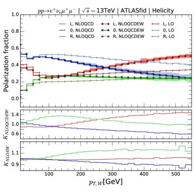
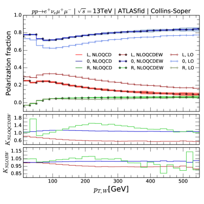
Figure 15: Transverse momentum distributions of the $W^{+}$ boson fiducial polarization fractions for the process $pp\to e^{+}\nu_{e}\,\mu^{+}\mu^{-}+X$ at the 13 TeV LHC with the ATLAS fiducial cuts. The left-hand-side plot is for the HE coordinate system, while the right-hand-side plot is for the CS coordinate system. The bands include PDF and scale uncertainties calculated at NLOQCD.

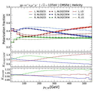
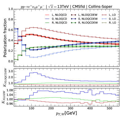
Figure 16: Same as Fig. 15 but for CMS fiducial cuts.

The CS coordinate system displays a complete different behavior. Except at some specific locations where the LO predictions are close to zero, the NLO $K$-factors are close to one for the right-handed polarization fraction $f_{R}$. The NLO corrections are constant at high $p_{T}$ for the longitudinal polarization fractions as well as for the left-handed polarization fractions. Again the NLO EW corrections can be sizable, e.g. close to $\pm 10\%$ for the $p_{T,Z}$ distribution of the polarization fractions using the ATLAS fiducial cuts.

The rapidity and pseudo-rapidity distributions of the $Z$ boson, shown in Fig. 19, Fig. 20, Fig. 21, and Fig. 22 display also the importance of the higher-order corrections. Except at the edges of each distribution, where the LO results are close to zero, the bulk of the NLO EW corrections is between $-20\%$ and $+10\%$. The total NLO corrections, including QCD effects, are about $+50\%$ for the left-handed polarization fraction in the bulk. On the edges of the distribution the $K$-factors can reach values of $2$ or $3$, again due to the smallness of the LO results. In all distributions the combined scale+PDF uncertainty is very small, as seen by the bands in all figures. They do not exceed $\simeq+5\%$.

Finally, it is important to note that the longitudinal fraction of a massive gauge boson decreases at large $p_{T,V}$ according to the equivalence theorem. This feature is seen for the fiducial longitudinal fraction $f_{0}$ in the helicity coordinate system, but not in the Collins-Soper system. As above mentioned, this is because the $z$ axis is aligned along the vector-boson direction of flight in the helicity system, but not in the Collins-Soper one. Therefore, the $f_{0}$ fraction in the Collins-Soper coordinate system is not the longitudinal fraction.

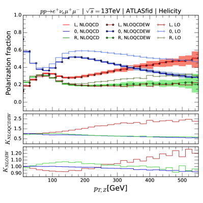
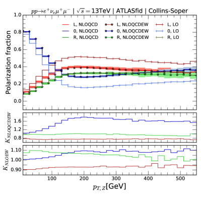
Figure 17: Same as Fig. 15 but for the $Z$ boson.

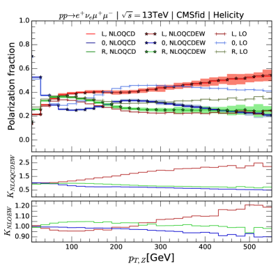
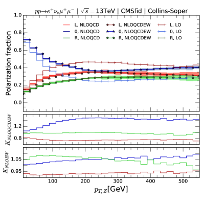
Figure 18: Same as Fig. 17 but for the CMS fiducial cuts.

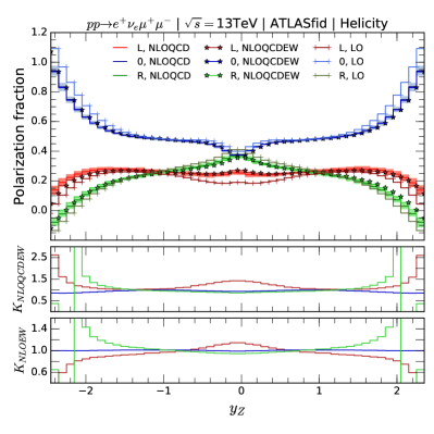
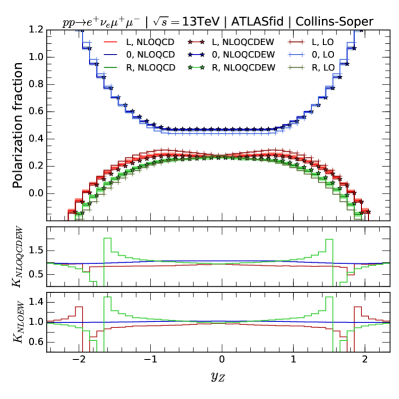
Figure 19: Same as Fig. 15 but for the rapidity distributions of the $Z$ polarization fractions.

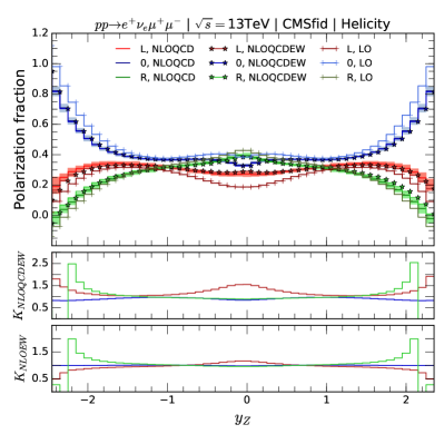
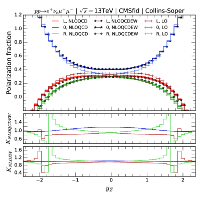
Figure 20: Same as Fig. 19 but for the CMS fiducial cuts.

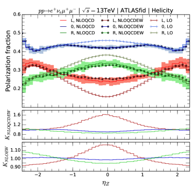
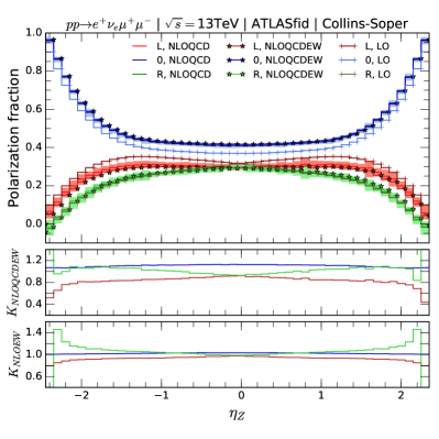
Figure 21: Same as Fig. 15 but for the pseudo-rapidity distributions of the $Z$ fiducial polarization fractions.

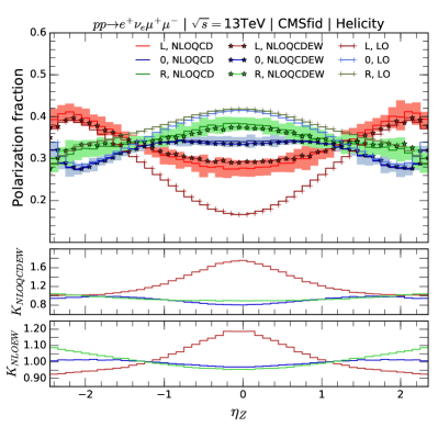
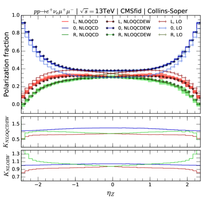
Figure 22: Same as Fig. 21 but for the CMS fiducial cuts.

6 Conclusions

We have presented in this paper an NLO analysis , including both QCD and EW corrections, of the fiducial angular coefficients and of the fiducial polarization fractions of the $W^{\pm}$ and $Z$ bosons in the process $pp\to e\nu\mu^{+}\mu^{-}$ at the 13 TeV LHC, using the fiducial phase space provided by the ATLAS and CMS experiments and in two different coordinate systems. The LO and NLO QCD predictions include off-shell effects, while the EW corrections have been calculated in the DPA. Comparing our predictions for the cross sections as well as for the kinematical distributions to the full NLO EW results, we find that the DPA predicts the quark-photon induced and the quark-antiquark corrections correctly. Very good agreement has been found for many kinematical distributions. In particular, the shape of the kinematical distributions is well reproduced by the DPA.

We have included the scale and PDF uncertainties, added linearly, in our predictions for the fiducial angular coefficients and for the fiducial polarization fractions. They have been found to be very small. The EW corrections are found to be significant, of about $-30\%$ to the NLO QCD predictions, in two angular coefficients $A_{3}$ and $A_{4}$ for the $Z$ boson, and they are mainly due to the EW corrections to the $Z$ decay into charged leptons. As $f_{L}$ and $f_{R}$ can be built out of $A_{4}$, significant EW corrections, of about $\pm 5\%$ to the NLO QCD results, are also found for these polarization fractions. Meanwhile, those EW corrections have been found very small for the $W^{\pm}$ bosons. We have also studied the transverse momenta, rapidity, and pseudo-rapidity distributions of the fiducial polarization fractions and we have found that the EW corrections can also be significant over the whole range of transverse momenta for $f_{L}^{Z}$ and $f_{R}^{Z}$. This happens for both the ATLAS and CMS fiducial cuts and in the two coordinate systems we have considered, namely the helicity and Collins-Soper coordinate systems.

We have observed that the fiducial polarization observables in the Collins-Soper coordinate system have unexpected behaviors such as negative fractions and not-decreasing longitudinal fraction at large transverse momentum values. Meanwhile, in the helicity system, the fiducial fractions are all positive and the longitudinal fraction decreases with large $p_{T,V}$ for both the $W$ and $Z$ bosons in accordance with the equivalence theorem. This can be understood because the $z$ axis is aligned along the vector-boson direction of flight in the helicity system, but not in the Collins-Soper one. Therefore, the fractions calculated in the helicity system are closer to the on-shell values.

This study also shows that it is easy to calculate the fiducial polarization observables. They can also be viewed as a simple way to characterize the three-dimensional polar-azimuthal angular distributions in terms of eight parameters, where three of them are very small and can be neglected. They share some common properties with the inclusive polarization observables and would enable theorists to perform precise comparisons with measurements without doing the template fitting step.

We therefore recommend that experimentalists provide measurements for these fiducial coefficients in the helicity coordinate system for both the $W$ and $Z$ bosons.

Appendix A NLO EW corrections in the DPA

We spell out here all necessary details of our NLO EW calculation in the DPA in such a way that the reader will have all information needed to reproduce our results. In order to achieve this, the on-shell mappings and the method for calculating NLO EW corrections have to be specified.

For the DPA LO, the OS mapping is done as follows. We first generate the exact kinematics, i.e. the momenta $(p_{1},p_{2},k_{i})$ with $i=1,4$ as defined in Section 2.2. The exact momenta of the two gauge bosons are $q_{1}$ and $q_{2}$ as defined in Eq. (4). The corresponding OS momenta $\hat{q}_{j}$ are calculated as follows. In the $WZ$ center-of-mass system, we choose

$$\vec{\hat{q}}_{1}=b\vec{q}_{1}.$$ (54)

We note that this choice is the same as the one used in Ref. Denner:2000bj . We then obtain, with $p_{1}^{\mu}=(E,0,0,E)$,

$$\hat{q}_{10} = \frac{M^{2}_{V_{1}}-M^{2}_{V_{2}}}{4E}+E,\quad\hat{q}_{20}=\frac{M^{2}_{V_{2}}-M^{2}_{V_{1}}}{4E}+E,$$

$$q_{10} = \frac{q_{1}^{2}-q_{2}^{2}}{4E}+E,\quad q_{20}=\frac{q_{2}^{2}-q_{1}^{2}}{4E}+E,$$

$$b = \sqrt{(\hat{q}^{2}_{10}-M^{2}_{V_{1}})/(q^{2}_{10}-q^{2}_{1})}.$$ (55)

Since the parameter $b$ must be real (otherwise we get complex momenta), we obtain the condition for the partonic energy

$$2E>M_{V_{1}}+M_{V_{2}},$$ (56)

which is equivalent to Eq. (10). The next step is to perform the decays $\hat{q}_{j}\to\hat{k}_{i_{1}}+\hat{k}_{i_{2}}$ to obtain the OS-projected momenta $\hat{k}_{i}$. They are first calculated in the rest frame of $V_{j}$ using two random numbers for each gauge boson and then boost back. This Monte-Carlo method is described in Ref. Berends:1994pv and is also implemented in the VBFNLO program, see the subroutine TwoBodyDecay0($R_{1}$, $R_{2}$, $\ldots$) there. In our code, the same random numbers $R_{1}$, $R_{2}$ used in generating $k_{i}$ are used for $\hat{k}_{i}$. The momenta of the initial partons are unchanged, i.e. $\hat{p}_{i}=p_{i}$, $i=1,2$. We call this method OS mapping R to distinguish with the OS mapping D method defined as follows. Following Ref. Denner:2000bj , the lepton momenta are calculated as

$$\hat{k}^{\mu}_{1} =ck^{\mu}_{1},\quad\hat{k}^{\mu}_{3}=dk^{\mu}_{3},\quad\hat{k}_{2}=\hat{q}_{1}-ck_{1},\quad\hat{k}_{4}=\hat{q}_{2}-dk_{3},$$

$$c =\frac{M^{2}_{V_{1}}}{2\hat{q}_{1}k_{1}},\quad d=\frac{M^{2}_{V_{2}}}{2\hat{q}_{2}k_{3}}.$$ (57)

A comparison of these two methods for the cross section at DPA LO is presented in Table 9. The results presented in this paper are obtained using the OS mapping R.

Cut	Process	LO [fb]	DPA mapping R [fb]	DPA mapping D [fb]
ATLAS fid.	$e^{+}\nu_{e}\mu^{+}\mu^{-}$	$19.344[2]$	$18.740[2]$	$18.960[2]$
ATLAS fid.	$e^{-}\bar{\nu}_{e}\mu^{+}\mu^{-}$	$13.001[1]$	$12.987[1]$	$12.763[1]$
CMS fid.	$e^{+}\nu_{e}\mu^{+}\mu^{-}$	$24.6225[4]$	$23.510[2]$	$23.922[2]$
CMS fid.	$e^{-}\bar{\nu}_{e}\mu^{+}\mu^{-}$	$16.3205[2]$	$16.157[1]$	$15.847[1]$

Table 9: Born cross sections in fb obtained using the full matrix elements and also the DPA matrix elements with the OS mapping R and OS mapping D methods (see text). The numbers in square brackets represent the statistical error.

The OS-projected momenta are used to calculate the DPA matrix elements. However, for kinematical cuts and distributions, we use the exact kinematics for the LO-like phase space. The OS-projected momenta can also be used here but we have checked that using exact momenta for cuts gives better agreement with the full LO results. For a real-emission phase space with one extra particle, it is more complicated because there are tilde kinematics introduced by the dipole-subtraction method. Here we have to use the OS-projected momenta everywhere, i.e. for the matrix elements, cuts, and distributions. This point will be discussed in detail below.

The virtual EW corrections are calculated as in Ref. Baglio:2013toa and hence there is no need to repeat it here. The kinematics are the same as for the DPA LO. As done in Ref. Baglio:2013toa , we have checked that the virtual corrections including the endpoint contribution (also called I operator) defined in Refs. Dittmaier:1999mb ; Basso:2015gca to the decays are UV and IR finite. Mass regularization has been used and checks have been performed to make sure that the results are independent of the masses of the light fermions, i.e. all but the top quark.

For the $\delta\mathcal{A}_{\text{rad,DPA}}^{\bar{q}q^{\prime}\to V_{1}V_{2}\to 4l\gamma}$ contribution in Eq. (12), there are three terms. For the first term, the photon is radiated from the process $\bar{q}q^{\prime}\to V_{1}V_{2}$. This contains IR divergences needed to cancel with the corresponding term in the virtual corrections. The OS-projected momenta are calculated as follows. First, the exact kinematics for the process $\bar{q}q^{\prime}\to 4l+\gamma(k_{\gamma})$ are generated and the momenta $q_{1}=k_{1}+k_{2}$, $q_{2}=k_{3}+k_{4}$ for the intermediate gauge bosons are calculated. We then boost to the center-of-mass system of the two gauge bosons and calculate $\hat{q}_{j}$ as above. The OS-projected momenta for the leptons are calculated from $\hat{q}_{j}$ using the OS mapping D method. Using the OS mapping R method should work as well, but we have not tried to do this. After this, all momenta can be boosted back to the partonic or hadronic CMS as needed. The momenta of the initial partons and of the photon are unchanged. Since we use the dipole-subtraction method, there are subtraction terms involved. The amplitude in each of these terms is written in a factorized form similar to the DPA LO one. The OS-projected momenta for those amplitudes are calculated as follows. First, the tilde momenta, defined in Ref. Dittmaier:1999mb , corresponding to the reduced process $\bar{q}q^{\prime}\to V_{1}V_{2}$ are calculated as in Ref. Baglio:2013toa using the OS momenta $\hat{q}_{j}$. These tilde momenta are OS by construction, i.e. $\tilde{q}_{j}^{2}=M_{V_{j}}^{2}$. We then generate the OS momenta for the leptons from $\tilde{q}_{j}$ using Eq. (57) with $k_{1}$ and $k_{3}$ now chosen to be $\hat{k}_{1}$ and $\hat{k}_{3}$. We have checked that this choice gives an IR-safe result. It is noted that we use the same factor $1/(Q_{1}Q_{2})$ calculated from the exact momenta for all subtraction terms. For the kinematical cuts and distributions of the subtraction terms, we use the OS-projected momenta that enter the reduced amplitudes there. To cancel the IR divergences, we have to use the OS-projected momenta for cuts and distributions of the parent $N+1$ contribution. The same choice is used for the subtraction terms of the radiative decays discussed next.

For the second (or third) term in the RHS of Eq. (12) we have to focus on the radiative decay $V_{1}\to l_{1}l_{2}\gamma$. The phase space is generated in the same way as for the DPA LO, but we have to replace the LO decay $V_{1}\to l_{1}l_{2}$ by the radiative one. In our code, we have to call the subroutine ThreeBodyDecay0() of the VBFNLO program, which uses five random numbers to generate three Euler angles and two final-state particle energies. This routine is called two times: First to calculate the exact momenta and the phase-space Jacobian, second to calculate the OS-projected momenta using the $\hat{q}_{j}$ as described above. The same set of random numbers is used in both times. The other decay $V_{2}\to l_{3}l_{4}$ is calculated exactly as for the DPA LO. From this one can see that the OS mapping R method is very general and can be easily generalized for more complicated processes. We have also found another method to calculate the OS-projected momenta, similar to the OS mapping D method but for $1\to 3$ decays this time. This can be done as follows. We choose

$$\hat{k}_{i}^{\mu} =ck_{i}^{\mu},\quad i=1,2,\quad\hat{k}_{\gamma}=\hat{q}_{1}-c(\hat{k}_{1}+\hat{k}_{2}),$$

$$c =\frac{2(k_{1}+k_{2})\hat{q}_{1}-2\sqrt{[(k_{1}+k_{2})\hat{q}_{1}]^{2}-2(k_{1}k_{2})M^{2}_{V_{1}}}}{4k_{1}k_{2}},$$ (58)

where we have to take the minus sign solution for $c$ because the plus sign solution makes $(\hat{k}_{1}+\hat{k}_{\gamma})^{2}+(\hat{k}_{2}+\hat{k}_{\gamma})^{2}$ negative. We have also proved that the argument of the square root function is always positive when the DPA condition $(q_{1}+q_{2})^{2}>(M_{V_{1}}+M_{V_{2}})^{2}$ is satisfied. We call this OS mapping T method . We have checked that both choices give similar results and a comparison is presented in Table 10. The final NLO EW results of this paper are calculated using the OS mapping R method.

Cut	Process	$W$ (map. R) [fb]	$W$ (map. T) [fb]	$Z$ (map. R) [fb]	$Z$ (map. T) [fb]
ATLAS fid.	$e^{+}\nu_{e}\mu^{+}\mu^{-}$	$-0.1326[3]$	$-0.1283[8]$	$-0.7803[9]$	$-0.7651[10]$
ATLAS fid.	$e^{-}\bar{\nu}_{e}\mu^{+}\mu^{-}$	$-0.0813[2]$	$-0.0796[4]$	$-0.5262[5]$	$-0.5163[6]$
CMS fid.	$e^{+}\nu_{e}\mu^{+}\mu^{-}$	$-0.1451[5]$	$-0.1388[6]$	$-0.4090[6]$	$-0.4032[9]$
CMS fid.	$e^{-}\bar{\nu}_{e}\mu^{+}\mu^{-}$	$-0.0869[3]$	$-0.0843[7]$	$-0.2699[7]$	$-0.2693[7]$

Table 10: Cross sections in fb of the second ($W$) and third ($Z$) terms in the RHS of Eq. (12) with subtraction terms obtained using the DPA matrix elements with the OS mapping R and OS mapping T methods (see text). The numbers in square brackets represent the statistical error.

We now describe how the corresponding subtraction terms are calculated. For $Z(\hat{q}_{2})\to\mu^{+}(\hat{k}_{3})+\mu^{-}(\hat{k}_{4})+\gamma(\hat{k}_{\gamma})$ decay, the photon can only be radiated off the final state leptons. The subtraction term is calculated in a straightforward way using the method of Ref. Dittmaier:1999mb . For $W^{+}(\hat{q}_{2})\to e^{+}(\hat{k}_{1})+\nu_{e}(\hat{k}_{2})+\gamma(\hat{k}_{\gamma})$ decay, it is more complicated because the photon can be radiated from the initial-state $W$ boson. The method of Ref. Dittmaier:1999mb cannot be applied here because it is for $2\to n$ processes. Fortunately, the subtraction method for $1\to n$ decay processes has been worked out in Ref. Basso:2015gca and can be directly used here. The tilde momenta calculated from the hat ones are all on-shell by construction and hence no further OS projection is needed. As before, the same factor $1/(Q_{1}Q_{2})$ calculated from the exact momenta is used for all subtraction terms here as well. Concerning cross check, we have performed two independent calculations and checked that the soft and collinear limits work.

For the last term defined in Eq. (13), the central piece is the factor $\delta A_{\text{ind}}^{q\gamma\to V_{1}V_{2}q^{\prime}}$ which has been calculated in Ref. Baglio:2013toa and is therefore taken over. For the LO decay factors, they are calculated as for the DPA LO term, using the OS mapping R method to get the momenta. Same as for the above photon-emission corrections involving subtraction terms, we use the OS-projected momenta for the kinematical cuts and distributions of the subtraction terms and of the parent $N+1$ contribution.

Appendix B Kinematical distributions: $W^{-}Z$ channel

We present in this appendix the kinematical distributions for the process $pp\to e^{-}\bar{\nu}_{e}\mu^{+}\mu^{-}+X$. They are very similar to the kinematical distributions of the process $pp\to e^{+}\nu_{e}\mu^{+}\mu^{-}+X$ presented in Section 4.2, hence we do not repeat our analysis and just display the plots. Plots for the ATLAS fiducial cuts are displayed in Fig. 23, Fig. 24, Fig. 25, Fig. 26, and Fig. 27. Plots for the CMS fiducial cuts are presented in Fig. 28, Fig. 29, Fig. 30, Fig. 31, and Fig. 32.

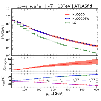
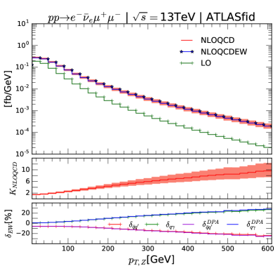
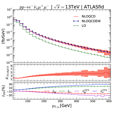
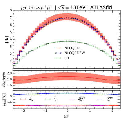
Figure 23: Distributions of the transverse momentum of the $e^{-}\nu_{e}$ (top left) and $\mu^{+}\mu^{-}$ (top right) systems and of the neutrino (bottom left) in the processes $pp\to e^{-}\nu_{e}\,\mu^{+}\mu^{-}+X$ at the 13 TeV LHC with the ATLAS fiducial cuts. Rapidity distribution of the $\mu^{+}\mu^{-}$ system is also displayed at the bottom right corner. The upper panels show the absolute values of the cross sections at LO (in green), NLO QCD (red), and NLO QCD+EW (blue). The middle panels display the ratio of the NLO QCD cross sections to the corresponding LO ones. The bands indicate the total theoretical uncertainty calculated as a linear sum of PDF and scale uncertainties at NLO QCD. The bottom panels show the NLO EW corrections (see text) calculated using DPA relative to the full LO (marked with plus signs) and DPA LO cross sections.

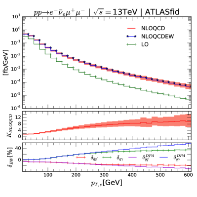
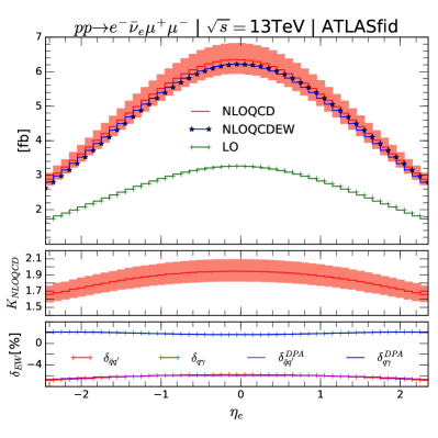
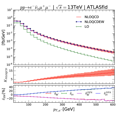
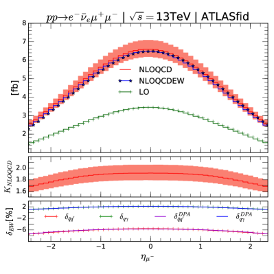
Figure 24: Same as Fig. 23 but for the transverse momentum and pseudo-rapidity distributions of the positron (top row) and the muon (bottom row).

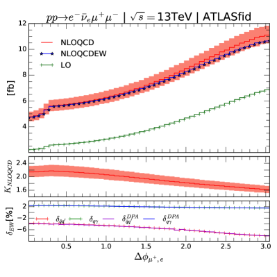
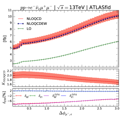
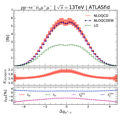
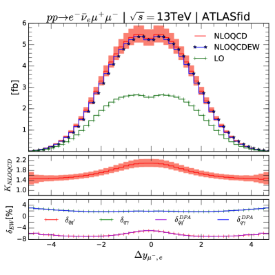
Figure 25: Same as Fig. 23 but for the azimuthal-angle difference (top row) and the rapidity difference (bottom row) between the $\mu^{+}$ and $e^{-}$ (left column) and between the $\mu^{-}$ and $e^{-}$ (right column).

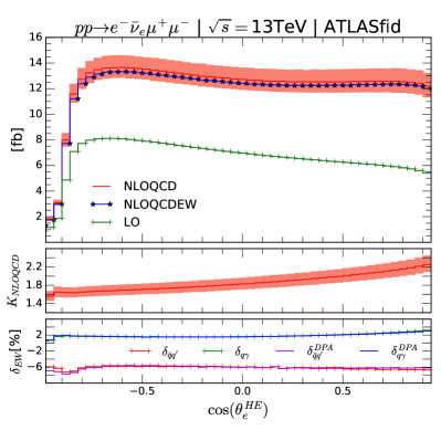
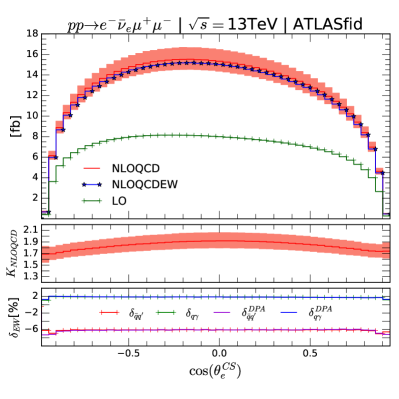
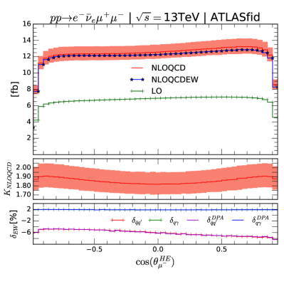
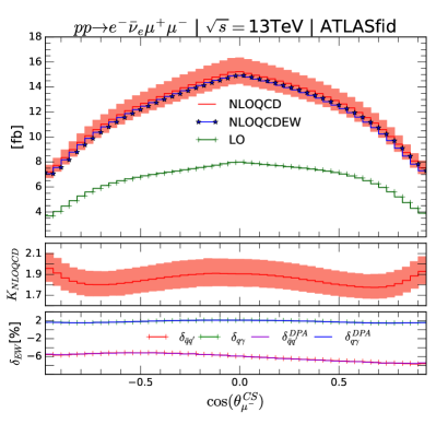
Figure 26: Same as Fig. 23 but for the $\cos\theta$ distributions of the electron (top row) calculated in the Helicity (left) and Collins-Soper (right) coordinate systems. The same distributions for the muon are shown in the bottom row.

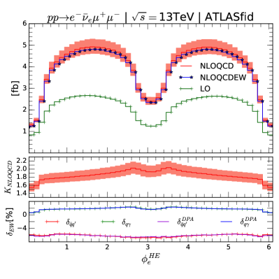
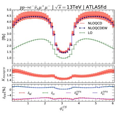
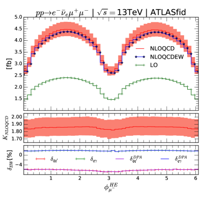
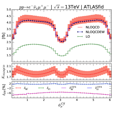
Figure 27: Same as Fig. 23 but for the azimuthal-angle distributions of the electron (top row) calculated in the Helicity (left) and Collins-Soper (right) coordinate systems. The same distributions for the muon are shown in the bottom row.

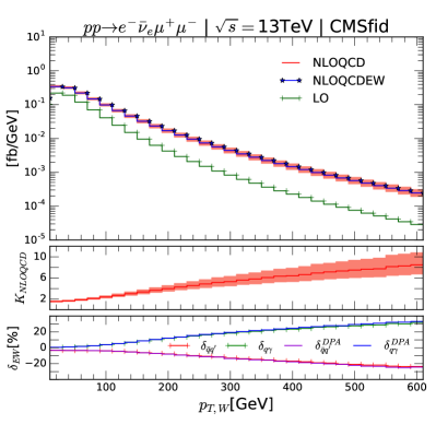
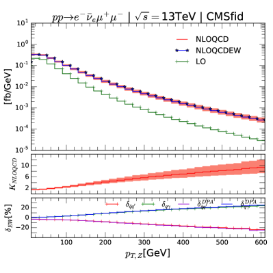
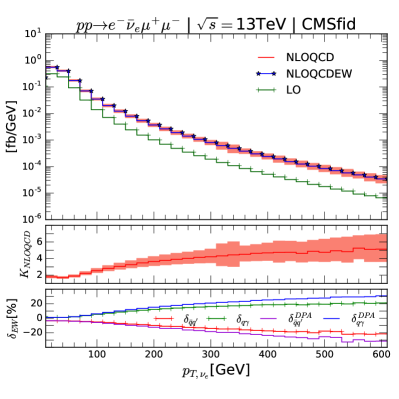
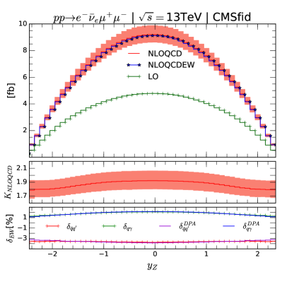
Figure 28: Same as Fig. 23 but with the CMS fiducial cuts.

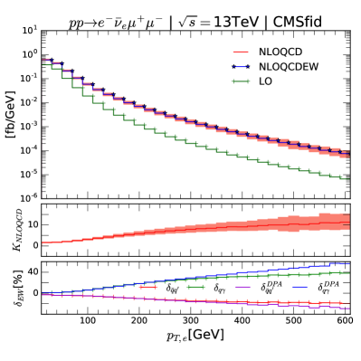
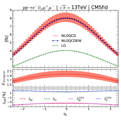
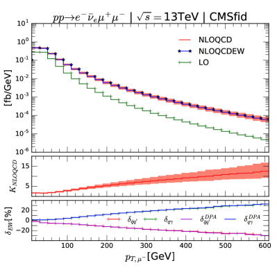
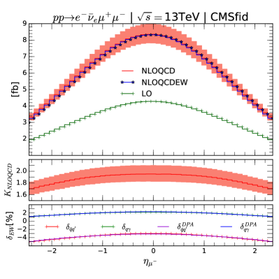
Figure 29: Same as Fig. 24 but with the CMS fiducial cuts.

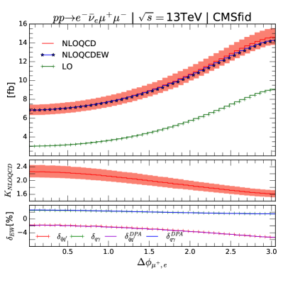
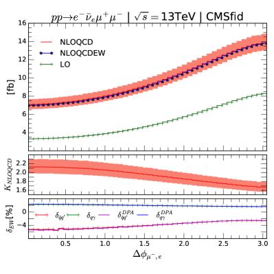
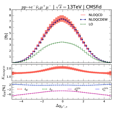
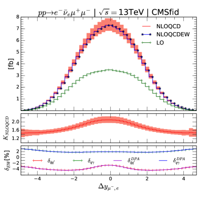
Figure 30: Same as Fig. 25 but with the CMS fiducial cuts.

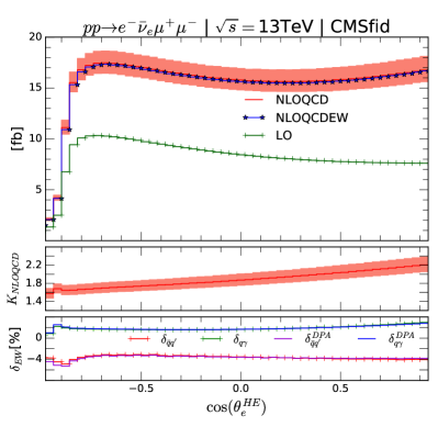
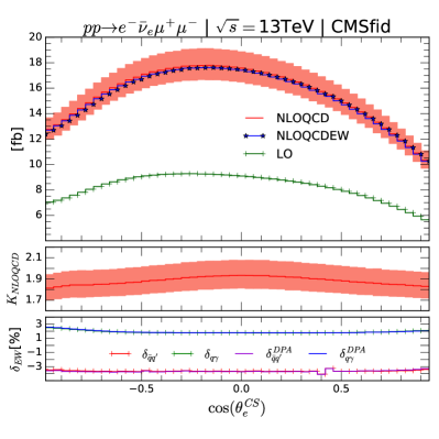
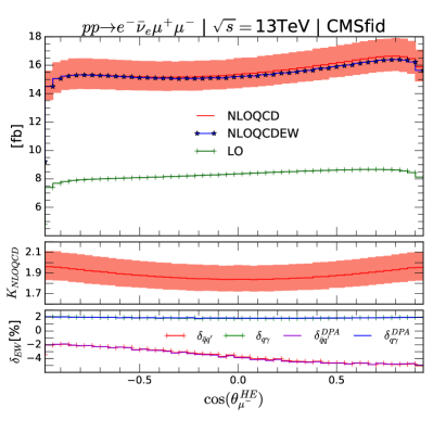
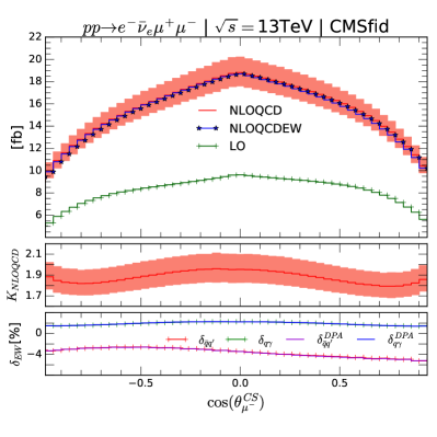
Figure 31: Same as Fig. 26 but with the CMS fiducial cuts.

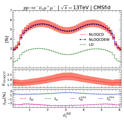
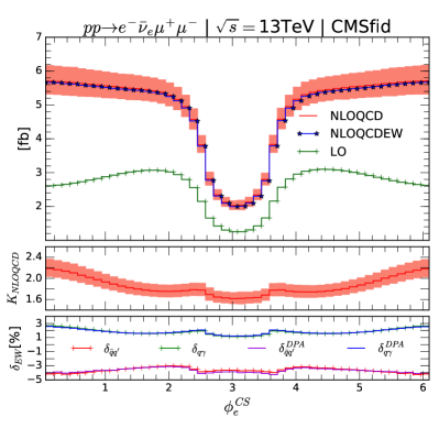
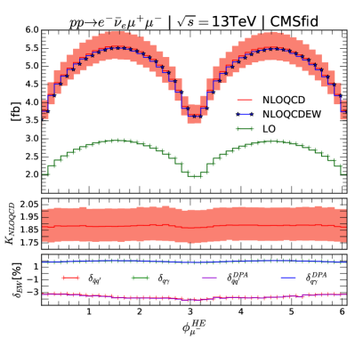
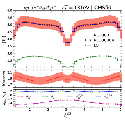
Figure 32: Same as Fig. 27 but with the CMS fiducial cuts.

Appendix C Numerical results for fiducial polarization observables: $W^{-}Z$ channel

We present in this appendix the numerical results for the fiducial polarization observables in the process $pp\to e^{-}\bar{\nu}_{e}\mu^{+}\mu^{-}+X$. The analysis is identical to that of the process $pp\to e^{+}\nu_{e}\mu^{+}\mu^{-}+X$ carried out in Section 5, hence we do not repeat ourselves and just present the numbers for the angular coefficients in Table 11, Table 12, Table 13, and Table 14; and for the polarization fractions in Table 15 and Table 16.

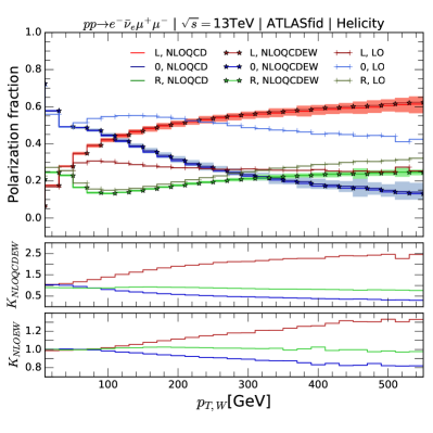
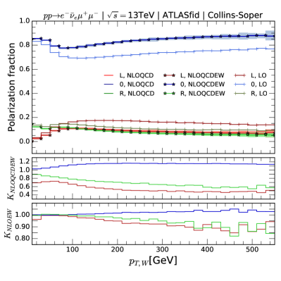
Figure 33: Transverse momentum distributions of the $W^{-}$ boson fiducial polarization fractions for the process $pp\to e^{-}\bar{\nu}_{e}\,\mu^{+}\mu^{-}+X$ at the 13 TeV LHC with the ATLAS fiducial cuts. The left-hand-side plot is for the HE coordinate system, while the right-hand-side plot is for the CS coordinate system. The bands include PDF and scale uncertainties calculated at NLOQCD.

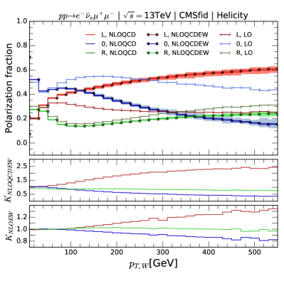
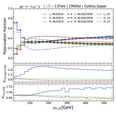
Figure 34: Same as Fig. 33 but with the CMS fiducial cuts.

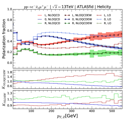
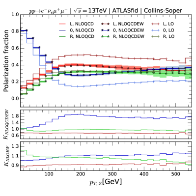
Figure 35: Same as Fig. 33 but for the $Z$ boson.

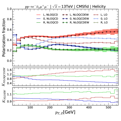
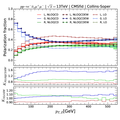
Figure 36: Same as Fig. 35 but with the CMS cuts.

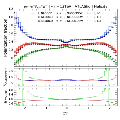
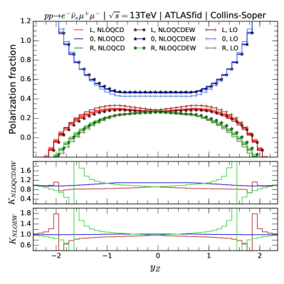
Figure 37: Same as Fig. 33 but for the rapidity distributions of the $Z$ fiducial polarization fractions.

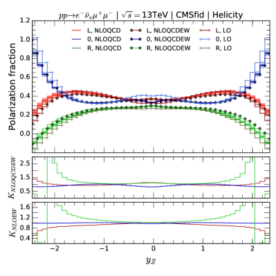
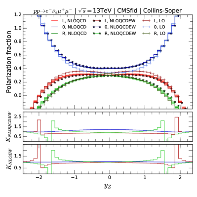
Figure 38: Same as Fig. 37 but with the CMS fiducial cuts.

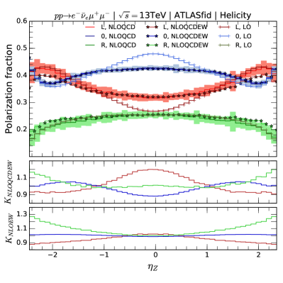
Figure 39: Same as Fig. 33 but for the pseudo-rapidity distributions of the $Z$ fiducial polarization fractions.

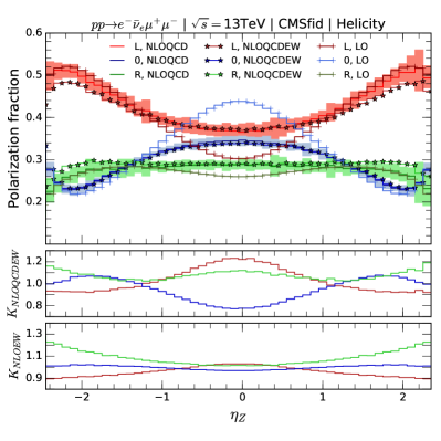
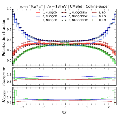
Figure 40: Same as Fig. 39 but with the CMS fiducial cuts.

The corresponding transverse momentum distributions of the fiducial polarization fractions can be found in Fig. 33, Fig. 34, Fig. 35, and Fig. 36. Rapidity and pseudo-rapidity distributions are displayed in Fig. 37, Fig. 38, Fig. 39, and Fig. 40.

C.1 Fiducial angular coefficients and polarization fractions: $W^{-}Z$ channel

Method	$A_{0}$	$A_{1}$	$A_{2}$	$A_{3}$	$A_{4}$	$A_{5}$	$A_{6}$	$A_{7}$
HE LO	$1.110(1)^{+2}_{-2}$	$-0.388(1)^{+2}_{-1}$	$-1.359(1)^{+2}_{-2}$	$-0.127(2)^{+2}_{-3}$	$-0.025(6)^{+2}_{-2}$	$0.0003(3)^{+1}_{-1}$	$0.003(0.2)^{+0.01}_{-0.1}$	$0.011(0.3)^{+0.05}_{-0}$
HE NLOEW	$1.107$	$-0.385$	$-1.372$	$-0.126$	$-0.021$	$0.002$	$0.006$	$0.010$
HE NLOQCD	$1.029(2)^{+9}_{-9}$	$-0.425(1)^{+2}_{-2}$	$-1.361(2)^{+3}_{-5}$	$-0.227(2)^{+7}_{-7}$	$0.175(6)^{+17}_{-16}$	$0.001(1)^{+0.04}_{-0.1}$	$0.002(1)^{+0.1}_{-0.3}$	$0.002(1)^{+1}_{-0.5}$
HE NLOQCDEW	$1.026$	$-0.424$	$-1.368$	$-0.228$	$0.181$	$0.001$	$0.003$	$0.001$
CS LO	$1.578(2)^{+1}_{-1}$	$0.214(1)^{+1}_{-1}$	$-0.893(1)^{+2}_{-2}$	$0.139(2)^{+2}_{-1}$	$-0.123(8)^{+3}_{-3}$	$-0.003(0.2)^{+0.1}_{-0.1}$	$-0.003(0.2)^{+0.1}_{-0.1}$	$-0.011(0.3)^{+0}_{-0.05}$
CS NLOEW	$1.580$	$0.213$	$-0.902$	$0.141$	$-0.124$	$-0.004$	$-0.005$	$-0.010$
CS NLOQCD	$1.650(2)^{+4}_{-4}$	$0.156(1)^{+4}_{-4}$	$-0.743(3)^{+9}_{-9}$	$0.356(5)^{+18}_{-17}$	$-0.112(6)^{+1}_{-1}$	$-0.001(0.5)^{+0.1}_{-0.1}$	$-0.002(0.5)^{+0.2}_{-0.2}$	$-0.002(1)^{+0.5}_{-1}$
CS NLOQCDEW	$1.653$	$0.154$	$-0.744$	$0.362$	$-0.112$	$-0.002$	$-0.003$	$-0.001$

Table 11: Fiducial angular coefficients of the $e^{-}$ distribution for the process $pp\to e^{-}\bar{\nu}_{e}\,\mu^{+}\mu^{-}+X$ at LO, NLO EW, NLO QCD and NLO QCD+EW at the 13 TeV LHC with the ATLAS fiducial cuts. Results are presented for two coordinate systems: the helicity (HE) and Collins-Soper (CS) coordinate systems. The PDF uncertainties (in parenthesis) and the scale uncertainties are provided for the LO and NLO QCD results, all given on the last digit of the central prediction.

Method	$A_{0}$	$A_{1}$	$A_{2}$	$A_{3}$	$A_{4}$	$A_{5}$	$A_{6}$	$A_{7}$
HE LO	$0.989(1)^{+1}_{-1}$	$-0.326(1)^{+1}_{-1}$	$-0.736(1)^{+1}_{-1}$	$-0.013(1)^{+0.1}_{-0.1}$	$0.061(1)^{+0.03}_{-0}$	$0.003(0.2)^{+0.1}_{-0.04}$	$0.009(0.2)^{+0}_{-0.1}$	$0.006(0.2)^{+0}_{-0.1}$
HE NLOEW	$0.992$	$-0.330$	$-0.748$	$-0.008$	$0.039$	$0.004$	$0.011$	$0.006$
HE NLOQCD	$0.950(1)^{+4}_{-5}$	$-0.323(1)^{+4}_{-3}$	$-0.754(1)^{+1}_{-1}$	$-0.016(1)^{+0.2}_{-0.2}$	$0.062(1)^{+1}_{-1}$	$0.001(0.5)^{+0.1}_{-0.05}$	$0.005(1)^{+0.3}_{-0.2}$	$0.004(0.4)^{+0.3}_{-0.2}$
HE NLOQCDEW	$0.951$	$-0.326$	$-0.760$	$-0.013$	$0.050$	$0.002$	$0.006$	$0.004$
CS LO	$1.251(1)^{+1}_{-2}$	$0.313(1)^{+2}_{-2}$	$-0.477(1)^{+1}_{-1}$	$0.050(0.2)^{+0.1}_{-0.1}$	$0.048(2)^{+0.1}_{-0}$	$-0.004(0.3)^{+0.1}_{-0}$	$-0.010(0.2)^{+0.1}_{-0.1}$	$-0.006(0.2)^{+0.1}_{-0}$
CS NLOEW	$1.263$	$0.308$	$-0.480$	$0.032$	$0.030$	$-0.005$	$-0.011$	$-0.006$
CS NLOQCD	$1.271(1)^{+3}_{-4}$	$0.268(1)^{+3}_{-3}$	$-0.436(2)^{+3}_{-3}$	$0.055(1)^{+1}_{-1}$	$0.036(1)^{+1}_{-1}$	$-0.003(0.5)^{+0.2}_{-0.1}$	$-0.005(1)^{+0.1}_{-0.4}$	$-0.004(0.4)^{+0.2}_{-0.2}$
CS NLOQCDEW	$1.278$	$0.265$	$-0.436$	$0.046$	$0.026$	$-0.003$	$-0.005$	$-0.004$

Table 12: Same as Table 11 but for the $\mu^{-}$ distribution.

Method	$A_{0}$	$A_{1}$	$A_{2}$	$A_{3}$	$A_{4}$	$A_{5}$	$A_{6}$	$A_{7}$
HE LO	$1.006(1)^{+2}_{-2}$	$-0.079(2)^{+3}_{-3}$	$-0.742(2)^{+4}_{-3}$	$-0.156(3)^{+3}_{-3}$	$-0.002(7)^{+2}_{-2}$	$0.0005(3)^{+0}_{-1}$	$0.003(0.2)^{+0}_{-0.03}$	$0.010(0.2)^{+0.03}_{-0.02}$
HE NLOEW	$1.003$	$-0.072$	$-0.742$	$-0.156$	$0.001$	$0.002$	$0.006$	$0.009$
HE NLOQCD	$0.949(1)^{+6}_{-7}$	$-0.126(2)^{+3}_{-3}$	$-0.671(2)^{+7}_{-7}$	$-0.249(3)^{+7}_{-6}$	$0.192(7)^{+17}_{-16}$	$0.001(0.4)^{+0.1}_{-0.1}$	$0.002(0.4)^{+0.1}_{-0.2}$	$0.002(0.5)^{+0.5}_{-0.5}$
HE NLOQCDEW	$0.947$	$-0.122$	$-0.671$	$-0.250$	$0.195$	$0.001$	$0.003$	$0.001$
CS LO	$1.013(3)^{+4}_{-5}$	$0.216(1)^{+1}_{-1}$	$-0.735(1)^{+1}_{-1}$	$0.182(2)^{+1}_{-1}$	$-0.131(9)^{+4}_{-4}$	$-0.002(0.2)^{+0.01}_{-0.1}$	$-0.003(0.2)^{+0.1}_{-0}$	$-0.010(0.2)^{+0.02}_{-0.03}$
CS NLOEW	$1.007$	$0.214$	$-0.739$	$0.184$	$-0.133$	$-0.003$	$-0.005$	$-0.009$
CS NLOQCD	$1.067(2)^{+3}_{-4}$	$0.157(1)^{+4}_{-4}$	$-0.554(4)^{+14}_{-14}$	$0.388(5)^{+17}_{-16}$	$-0.123(6)^{+1}_{-0.4}$	$-0.001(0.5)^{+0.1}_{-0.1}$	$-0.002(0.4)^{+0.1}_{-0.1}$	$-0.002(0.5)^{+0.5}_{-0.5}$
CS NLOQCDEW	$1.064$	$0.155$	$-0.554$	$0.391$	$-0.124$	$-0.001$	$-0.003$	$-0.001$

Table 13: Same as Table 11 but with the CMS fiducial cuts.

Method	$A_{0}$	$A_{1}$	$A_{2}$	$A_{3}$	$A_{4}$	$A_{5}$	$A_{6}$	$A_{7}$
HE LO	$0.798(1)^{+2}_{-3}$	$-0.288(1)^{+1}_{-1}$	$-0.603(1)^{+1}_{-2}$	$-0.017(1)^{+0.1}_{-0.1}$	$0.072(1)^{+0.04}_{-0}$	$0.003(0.2)^{+0.1}_{-0.04}$	$0.009(0.4)^{+0}_{-0.05}$	$0.006(0.2)^{+0.04}_{-0.01}$
HE NLOEW	$0.795$	$-0.297$	$-0.606$	$-0.012$	$0.048$	$0.004$	$0.011$	$0.006$
HE NLOQCD	$0.739(1)^{+7}_{-7}$	$-0.312(1)^{+3}_{-2}$	$-0.609(1)^{+0.4}_{-0.5}$	$-0.018(1)^{+0.2}_{-0.1}$	$0.069(1)^{+1}_{-1}$	$0.001(1)^{+0.2}_{-0.1}$	$0.005(0.5)^{+0.3}_{-0.3}$	$0.004(0.4)^{+0.3}_{-0.1}$
HE NLOQCDEW	$0.737$	$-0.317$	$-0.611$	$-0.015$	$0.057$	$0.001$	$0.006$	$0.004$
CS LO	$1.113(1)^{+0.4}_{-0.03}$	$0.382(1)^{+3}_{-2}$	$-0.291(1)^{+1}_{-1}$	$0.061(0.2)^{+0.1}_{-0.03}$	$0.050(2)^{+0.1}_{-0.01}$	$-0.005(0.3)^{+0.1}_{-0}$	$-0.010(0.3)^{+0.1}_{-0.1}$	$-0.006(0.2)^{+0.01}_{-0.04}$
CS NLOEW	$1.128$	$0.377$	$-0.276$	$0.042$	$0.032$	$-0.005$	$-0.011$	$-0.006$
CS NLOQCD	$1.176(1)^{+4}_{-3}$	$0.329(1)^{+3}_{-3}$	$-0.176(2)^{+8}_{-8}$	$0.063(1)^{+1}_{-1}$	$0.037(1)^{+1}_{-1}$	$-0.003(1)^{+0.3}_{-0.02}$	$-0.005(0.4)^{+0.3}_{-0.3}$	$-0.004(0.4)^{+0.2}_{-0.2}$
CS NLOQCDEW	$1.184$	$0.326$	$-0.167$	$0.053$	$0.028$	$-0.003$	$-0.005$	$-0.004$

Table 14: Same as Table 12 but with the CMS fiducial cuts.

Method	$f^{W^{-}}_{L}$	$f^{W^{-}}_{0}$	$f^{W^{-}}_{R}$	$f^{Z}_{L}$	$f^{Z}_{0}$	$f^{Z}_{R}$
HE LO	$0.216(1)^{+0.1}_{-0.05}$	$0.555(1)^{+1}_{-1}$	$0.229(2)^{+1}_{-1}$	$0.324(1)^{+0.4}_{-0.3}$	$0.494(0.4)^{+1}_{-1}$	$0.181(1)^{+0.3}_{-0.4}$
HE NLOEW	$0.218$	$0.554$	$0.228$	$0.298$	$0.496$	$0.206$
HE NLOQCD	$0.286(2)^{+7}_{-6}$	$0.515(1)^{+4}_{-5}$	$0.199(1)^{+2}_{-2}$	$0.334(1)^{+2}_{-2}$	$0.475(0.5)^{+2}_{-2}$	$0.191(1)^{+1}_{-1}$
HE NLOQCDEW	$0.289$	$0.513$	$0.198$	$0.321$	$0.475$	$0.204$
CS LO	$0.075(2)^{+0.5}_{-1}$	$0.789(1)^{+1}_{-1}$	$0.136(2)^{+1}_{-1}$	$0.243(2)^{+1}_{-0.3}$	$0.625(1)^{+1}_{-1}$	$0.132(2)^{+0.3}_{-0.3}$
CS NLOEW	$0.074$	$0.790$	$0.136$	$0.220$	$0.632$	$0.149$
CS NLOQCD	$0.059(1)^{+1}_{-1}$	$0.825(1)^{+2}_{-2}$	$0.115(2)^{+1}_{-1}$	$0.224(1)^{+1}_{-1}$	$0.636(1)^{+2}_{-2}$	$0.140(1)^{+2}_{-1}$
CS NLOQCDEW	$0.059$	$0.826$	$0.115$	$0.211$	$0.639$	$0.150$

Table 15: $W^{-}$ and $Z$ fiducial polarization fractions in the process $pp\to e^{-}\nu_{e}\,\mu^{+}\mu^{-}+X$ at LO, NLO EW, NLO QCD and NLO QCD+EW at the 13 TeV LHC with the ATLAS fiducial cuts. Results are presented for two coordinate systems: the helicity (HE) and Collins-Soper (CS) coordinate systems. The PDF uncertainties (in parenthesis) and the scale uncertainties are provided for the LO and NLO QCD results, all given on the last digit of the central prediction.

Method	$f^{W^{-}}_{L}$	$f^{W^{-}}_{0}$	$f^{W^{-}}_{R}$	$f^{Z}_{L}$	$f^{Z}_{0}$	$f^{Z}_{R}$
HE LO	$0.248(2)^{+0.02}_{-0}$	$0.503(1)^{+1}_{-1}$	$0.249(2)^{+1}_{-1}$	$0.384(1)^{+1}_{-1}$	$0.399(1)^{+1}_{-1}$	$0.217(1)^{+1}_{-1}$
HE NLOEW	$0.250$	$0.501$	$0.249$	$0.358$	$0.398$	$0.245$
HE NLOQCD	$0.311(2)^{+6}_{-6}$	$0.474(1)^{+3}_{-4}$	$0.215(2)^{+2}_{-2}$	$0.396(1)^{+3}_{-2}$	$0.369(0.5)^{+3}_{-4}$	$0.235(1)^{+1}_{-1}$
HE NLOQCDEW	$0.312$	$0.473$	$0.214$	$0.382$	$0.368$	$0.250$
CS LO	$0.214(2)^{+0.3}_{-0.2}$	$0.507(1)^{+2}_{-3}$	$0.279(3)^{+2}_{-2}$	$0.280(2)^{+0.1}_{-0.1}$	$0.557(1)^{+0.2}_{-0.02}$	$0.163(2)^{+0}_{-0.1}$
CS NLOEW	$0.215$	$0.504$	$0.281$	$0.256$	$0.564$	$0.180$
CS NLOQCD	$0.203(1)^{+1}_{-1}$	$0.533(1)^{+2}_{-2}$	$0.264(2)^{+1}_{-1}$	$0.249(1)^{+2}_{-2}$	$0.588(1)^{+2}_{-2}$	$0.163(1)^{+1}_{-1}$
CS NLOQCDEW	$0.203$	$0.532$	$0.265$	$0.236$	$0.592$	$0.171$

Table 16: Same as Table 15 but with the CMS fiducial cuts.

C.2 Distributions of fiducial polarization fractions: $W^{-}Z$ channel

Appendix D Off-shell and NLO EW correction effects on fiducial polarization observables

Here we would like to show the effects of various contributions including the $\bar{q}q^{\prime}$ annihilation channels at NLO EW, denoted as $\text{F-EW-}\bar{q}q^{\prime}$ where F means that the full LO amplitudes are used and the $\bar{q}q^{\prime}$ corrections are calculated as in Eq. (21), and similarly the quark-photon induced channels denoted as $\text{F-EW-}q\gamma$ with the quark-photon induced corrections calculated as in Eq. (22). Results for full LO (denoted F-LO) and for full LO plus NLO EW corrections (denoted F-EW) have been provided in Section 5.1, but are also included in the tables here for easy comparisons. It is noted that some results for the F-LO and the F-EW shown here are not identical as those in Section 5.1, but agree within the statistical error. This is because the full LO results here are obtained using our in-house code while the ones in Section 5.1 are calculated using the VBFNLO program.

Moreover, the DPA LO results, denoted as D-LO, are also shown. This enables one to see the off-shell effects at LO by comparing to the F-LO results. As discussed in Section 2.3, when we are looking at the polarization of a gauge boson, it is interesting to separate the EW corrections to the production part from those to the decay part. This is possible in our DPA framework because off-shell effects are absent. The EW corrections to the $W^{\pm}$ production part $\bar{q}q^{\prime}\to W^{\pm}\mu^{+}\mu^{-}$, defined in Eq. (25), are included in the D-EW-pV (where pV denotes production of $V$ boson) results presented here. Note that this includes EW corrections to the $\bar{q}q^{\prime}\to W^{\pm}Z$ part and also to the $Z\to\mu^{+}\mu^{-}$ decay. Same things apply to the EW corrections to the $Z$ production part $\bar{q}q^{\prime}\to e\nu_{e}Z$. To see these effects, one has to compare the D-EW-pV results to the corresponding D-LO results. The EW corrections to the decay $W\to e\nu_{e}$ or $Z\to\mu^{+}\mu^{-}$ are defined in Eq. (24). They can be seen by comparing the D-EW-dV (where dV denotes decay of $V$ boson) rows to the corresponding D-LO rows. Finally, the D-EW entries show the results of the DPA LO plus NLO EW corrections.

In Table 17 and Table 18 we show results of the $W$ and $Z$ angular coefficients for the $W^{+}Z$ channel with the ATLAS fiducial cuts, respectively. Similar results with the CMS cuts are provided in Table 19 and Table 20. Both $W^{+}$ and $Z$ polarization fractions with the ATLAS cuts are presented in Table 21 and with the CMS cuts in Table 22. Similar results for the $W^{-}Z$ channel are presented in Table 23 and Table 24 with the ATLAS cuts, in Table 25 and Table 26 with the CMS cuts, and finally in Table 27 and Table 28 for the polarization fractions.

We have a few remarks here on the results focusing on the fiducial angular coefficients. Looking at the results for $A_{5}$, $A_{6}$, and $A_{7}$ we see that the DPA LO results are all consistent with zero within the statistical error. Taking into the EW corrections to the decay part does not change this conclusion. However, the EW corrections to the production part have significant effects and make them non-vanishing, but the results are still very small. If full off-shell effects are included, they become non-vanishing as well, see the F-LO results. In general, the corrections to the decay part have negligible effects compared to those to the production part, except for the coefficients $A_{3}$ and $A_{4}$. In Table 24 for the $Z$ boson in the $W^{+}Z$ channel, we see that the EW corrections to the $Z$ decay have important effects and can change the DPA results by $30\%$. This explains why we see significant differences in the $A_{3}$ and $A_{4}$ coefficients when comparing the NLOQCD results to the NLOQCDEW ones for the case of the $Z$ boson in Section 5.1 and Appendix C. However, similar effects are not observed for the $W^{\pm}$ decays.

Method	$A_{0}$	$A_{1}$	$A_{2}$	$A_{3}$	$A_{4}$	$A_{5}$	$A_{6}$	$A_{7}$
HE F-LO	$1.026$	$-0.286$	$-1.315$	$-0.251$	$-0.447$	$-0.0021[3]$	$-0.0006[4]$	$-0.0036[3]$
$\text{HE F-EW-}\bar{q}q^{\prime}$	$1.034$	$-0.284$	$-1.321$	$-0.251$	$-0.451$	$-0.0040[4]$	$-0.0039[5]$	$0.0030[4]$
$\text{HE F-EW-}q\gamma$	$1.021$	$-0.286$	$-1.318$	$-0.253$	$-0.434$	$-0.0021[3]$	$-0.0006[4]$	$-0.0035[3]$
HE F-EW	$1.028$	$-0.284$	$-1.324$	$-0.252$	$-0.438$	$-0.0039[4]$	$-0.0038[5]$	$0.0029[4]$
HE D-LO	$1.023$	$-0.326$	$-1.404$	$-0.156$	$-0.445$	$-0.0001[3]$	$0.00001[39]$	$0.0001[3]$
$\text{HE D-EW-p}W^{+}$	$1.019$	$-0.325$	$-1.408$	$-0.155$	$-0.437$	$-0.0019[4]$	$-0.0033[4]$	$0.0070[3]$
$\text{HE D-EW-d}W^{+}$	$1.029$	$-0.326$	$-1.415$	$-0.154$	$-0.443$	$-0.00001[35]$	$0.00003[41]$	$0.0001[3]$
HE D-EW	$1.025$	$-0.325$	$-1.419$	$-0.152$	$-0.435$	$-0.0018[4]$	$-0.0033[4]$	$0.0070[4]$
CS F-LO	$1.397$	$0.229$	$-0.945$	$0.0025[3]$	$-0.613$	$-0.0002[4]$	$0.0021[4]$	$0.0036[3]$
$\text{CS F-EW-}\bar{q}q^{\prime}$	$1.399$	$0.225$	$-0.958$	$-0.0004[4]$	$-0.617$	$0.0006[4]$	$0.0059[5]$	$-0.0030[4]$
$\text{CS F-EW-}q\gamma$	$1.400$	$0.229$	$-0.940$	$0.010$	$-0.605$	$-0.0002[4]$	$0.0021[3]$	$0.0035[3]$
CS F-EW	$1.402$	$0.225$	$-0.952$	$0.0080[4]$	$-0.608$	$0.0006[4]$	$0.0059[4]$	$-0.0029[3]$
CS D-LO	$1.459$	$0.299$	$-0.971$	$-0.073$	$-0.544$	$-0.00001[38]$	$0.00003[38]$	$-0.0001[3]$
$\text{CS D-EW-p}W^{+}$	$1.460$	$0.298$	$-0.970$	$-0.069$	$-0.539$	$0.0009[6]$	$0.0038[4]$	$-0.0070[3]$
$\text{CS D-EW-d}W^{+}$	$1.465$	$0.298$	$-0.981$	$-0.075$	$-0.541$	$-0.00005[33]$	$0.00001[44]$	$-0.0001[3]$
CS D-EW	$1.466$	$0.297$	$-0.980$	$-0.071$	$-0.535$	$0.0009[5]$	$0.0038[4]$	$-0.0070[4]$

Table 17: Fiducial angular coefficients of the $e^{+}$ distribution for the process $pp\to e^{+}\nu_{e}\,\mu^{+}\mu^{-}+X$ at the 13 TeV LHC with the ATLAS fiducial cuts. Results are shown for full LO only, and also with the $\text{EW-}\bar{q}q^{\prime}$, $\text{EW-}q\gamma$, and the total EW correction included. Similarly, results for DPA LO only, and also with the EW-pV, EW-dV, and the total EW correction included are presented. The upper rows are for the helicity (HE) coordinate system, while the lower ones for the Collins-Soper (CS) coordinate system. The numbers in square brackets represent the statistical error, when it is significant.

Method	$A_{0}$	$A_{1}$	$A_{2}$	$A_{3}$	$A_{4}$	$A_{5}$	$A_{6}$	$A_{7}$
HE F-LO	$1.035$	$-0.303$	$-0.705$	$0.063$	$-0.017$	$-0.0068[4]$	$-0.0066[4]$	$0.0032[3]$
$\text{HE F-EW-}\bar{q}q^{\prime}$	$1.040$	$-0.305$	$-0.711$	$0.051$	$-0.021$	$-0.0076[5]$	$-0.0084[4]$	$0.0030[3]$
$\text{HE F-EW-}q\gamma$	$1.034$	$-0.306$	$-0.710$	$0.062$	$-0.016$	$-0.0067[4]$	$-0.0065[4]$	$0.0032[3]$
HE F-EW	$1.039$	$-0.307$	$-0.717$	$0.050$	$-0.020$	$-0.0074[5]$	$-0.0082[5]$	$0.0029[3]$
HE D-LO	$0.997$	$-0.265$	$-0.720$	$0.039$	$0.011$	$-0.00001[49]$	$0.00004[41]$	$0.0001[3]$
$\text{HE D-EW-p}Z$	$0.997$	$-0.266$	$-0.727$	$0.039$	$0.011$	$-0.0003[5]$	$-0.0012[4]$	$-0.0004[2]$
$\text{HE D-EW-d}Z$	$0.999$	$-0.267$	$-0.725$	$0.024$	$0.0078[2]$	$-0.00003[53]$	$0.00003[45]$	$0.0001[3]$
HE D-EW	$0.999$	$-0.268$	$-0.733$	$0.025$	$0.0078[2]$	$-0.0003[6]$	$-0.0013[5]$	$-0.0004[3]$
CS F-LO	$1.254$	$0.239$	$-0.488$	$-0.061$	$0.035$	$-0.0001[5]$	$0.010$	$-0.0032[3]$
$\text{CS F-EW-}\bar{q}q^{\prime}$	$1.260$	$0.236$	$-0.494$	$-0.054$	$0.023$	$0.0008[6]$	$0.012$	$-0.0030[3]$
$\text{CS F-EW-}q\gamma$	$1.259$	$0.238$	$-0.487$	$-0.059$	$0.035$	$-0.0001[5]$	$0.010$	$-0.0032[3]$
CS F-EW	$1.266$	$0.234$	$-0.493$	$-0.053$	$0.023$	$0.0007[6]$	$0.012$	$-0.0029[3]$
CS D-LO	$1.200$	$0.305$	$-0.519$	$-0.023$	$0.036$	$-0.0001[6]$	$0.00002[30]$	$-0.0001[3]$
$\text{CS D-EW-p}Z$	$1.205$	$0.302$	$-0.521$	$-0.023$	$0.036$	$0.0008[6]$	$0.0012[3]$	$0.0004[3]$
$\text{CS D-EW-d}Z$	$1.205$	$0.307$	$-0.522$	$-0.013$	$0.023$	$-0.00004[70]$	$0.00003[25]$	$-0.0001[2]$
CS D-EW	$1.209$	$0.303$	$-0.525$	$-0.013$	$0.023$	$0.0009[7]$	$0.0012[2]$	$0.0004[3]$

Table 18: Same as Table 17 but for $\mu^{-}$ distribution.

Method	$A_{0}$	$A_{1}$	$A_{2}$	$A_{3}$	$A_{4}$	$A_{5}$	$A_{6}$	$A_{7}$
HE F-LO	$0.897$	$0.088$	$-0.627$	$-0.373$	$-0.488$	$-0.0019[3]$	$-0.0008[3]$	$-0.0031[3]$
$\text{HE F-EW-}\bar{q}q^{\prime}$	$0.904$	$0.092$	$-0.629$	$-0.375$	$-0.493$	$-0.0037[3]$	$-0.0038[3]$	$0.0030[3]$
$\text{HE F-EW-}q\gamma$	$0.893$	$0.089$	$-0.622$	$-0.373$	$-0.475$	$-0.0018[3]$	$-0.0008[3]$	$-0.0030[3]$
HE F-EW	$0.899$	$0.092$	$-0.625$	$-0.374$	$-0.480$	$-0.0036[3]$	$-0.0038[3]$	$0.0029[3]$
HE D-LO	$0.900$	$0.037$	$-0.740$	$-0.258$	$-0.475$	$-0.00003[41]$	$0.0001[3]$	$0.0001[3]$
$\text{HE D-EW-p}W^{+}$	$0.898$	$0.039$	$-0.734$	$-0.258$	$-0.468$	$-0.0018[4]$	$-0.0030[3]$	$0.0064[3]$
$\text{HE D-EW-d}W^{+}$	$0.906$	$0.037$	$-0.747$	$-0.257$	$-0.474$	$-0.00003[41]$	$0.0001[3]$	$0.0001[3]$
HE D-EW	$0.903$	$0.040$	$-0.741$	$-0.257$	$-0.467$	$-0.0018[4]$	$-0.0030[3]$	$0.0065[3]$
CS F-LO	$0.760$	$0.196$	$-0.764$	$0.052$	$-0.723$	$-0.00002[28]$	$0.0021[4]$	$0.0031[3]$
$\text{CS F-EW-}\bar{q}q^{\prime}$	$0.758$	$0.191$	$-0.775$	$0.050$	$-0.728$	$0.0009[3]$	$0.0056[5]$	$-0.0030[3]$
$\text{CS F-EW-}q\gamma$	$0.759$	$0.196$	$-0.756$	$0.059$	$-0.714$	$-0.00001[27]$	$0.0020[4]$	$0.0030[3]$
CS F-EW	$0.758$	$0.192$	$-0.767$	$0.057$	$-0.719$	$0.0008[3]$	$0.0055[5]$	$-0.0029[3]$
CS D-LO	$0.839$	$0.280$	$-0.802$	$-0.027$	$-0.633$	$-0.0001[3]$	$-0.000003[432]$	$-0.0001[3]$
$\text{CS D-EW-p}W^{+}$	$0.835$	$0.278$	$-0.798$	$-0.022$	$-0.629$	$0.0008[4]$	$0.0035[5]$	$-0.0064[3]$
$\text{CS D-EW-d}W^{+}$	$0.843$	$0.279$	$-0.811$	$-0.028$	$-0.631$	$-0.0001[4]$	$0.00001[46]$	$-0.0002[3]$
CS D-EW	$0.839$	$0.277$	$-0.806$	$-0.023$	$-0.627$	$0.0008[4]$	$0.0036[5]$	$-0.0065[3]$

Table 19: Same as Table 17 but with the CMS fiducial cuts.

Method	$A_{0}$	$A_{1}$	$A_{2}$	$A_{3}$	$A_{4}$	$A_{5}$	$A_{6}$	$A_{7}$
HE F-LO	$0.858$	$-0.273$	$-0.570$	$0.068$	$-0.022$	$-0.0071[4]$	$-0.0064[3]$	$0.0028[3]$
$\text{HE F-EW-}\bar{q}q^{\prime}$	$0.858$	$-0.278$	$-0.568$	$0.056$	$-0.027$	$-0.0076[5]$	$-0.0078[3]$	$0.0024[3]$
$\text{HE F-EW-}q\gamma$	$0.855$	$-0.277$	$-0.576$	$0.067$	$-0.022$	$-0.0070[4]$	$-0.0063[3]$	$0.0028[3]$
HE F-EW	$0.855$	$-0.282$	$-0.574$	$0.055$	$-0.026$	$-0.0075[5]$	$-0.0077[3]$	$0.0024[3]$
HE D-LO	$0.806$	$-0.227$	$-0.592$	$0.039$	$0.012$	$0.00003[39]$	$0.0001[3]$	$0.0001[2]$
$\text{HE D-EW-p}Z$	$0.805$	$-0.229$	$-0.599$	$0.040$	$0.012$	$-0.0003[4]$	$-0.0011[3]$	$-0.0004[3]$
$\text{HE D-EW-d}Z$	$0.803$	$-0.232$	$-0.590$	$0.025$	$0.0082[3]$	$0.0001[4]$	$0.0001[3]$	$0.00002[18]$
HE D-EW	$0.802$	$-0.234$	$-0.596$	$0.026$	$0.0082[3]$	$-0.0002[5]$	$-0.0011[3]$	$-0.0004[3]$
CS F-LO	$1.128$	$0.296$	$-0.303$	$-0.069$	$0.038$	$-0.0003[4]$	$0.010$	$-0.0028[3]$
$\text{CS F-EW-}\bar{q}q^{\prime}$	$1.134$	$0.292$	$-0.294$	$-0.063$	$0.025$	$0.0005[4]$	$0.012$	$-0.0024[3]$
$\text{CS F-EW-}q\gamma$	$1.135$	$0.294$	$-0.298$	$-0.068$	$0.038$	$-0.0003[4]$	$0.010$	$-0.0028[3]$
CS F-EW	$1.141$	$0.291$	$-0.290$	$-0.062$	$0.025$	$0.0005[4]$	$0.012$	$-0.0024[3]$
CS D-LO	$1.065$	$0.378$	$-0.337$	$-0.022$	$0.039$	$-0.0001[4]$	$-0.00002[33]$	$-0.0001[2]$
$\text{CS D-EW-p}Z$	$1.071$	$0.374$	$-0.336$	$-0.022$	$0.039$	$0.0008[4]$	$0.0011[3]$	$0.0004[3]$
$\text{CS D-EW-d}Z$	$1.071$	$0.378$	$-0.325$	$-0.013$	$0.025$	$-0.0001[4]$	$-0.0001[3]$	$-0.00004[18]$
CS D-EW	$1.077$	$0.374$	$-0.324$	$-0.014$	$0.025$	$0.0008[3]$	$0.0011[4]$	$0.0004[3]$

Table 20: Same as Table 18 but with the CMS fiducial cuts.

Method	$f^{W^{+}}_{L}$	$f^{W^{+}}_{0}$	$f^{W^{+}}_{R}$	$f^{Z}_{L}$	$f^{Z}_{0}$	$f^{Z}_{R}$
HE F-LO	$0.355$	$0.513$	$0.132$	$0.222$	$0.518$	$0.261$
$\text{HE F-EW-}\bar{q}q^{\prime}$	$0.354$	$0.517$	$0.129$	$0.215$	$0.520$	$0.264$
$\text{HE F-EW-}q\gamma$	$0.353$	$0.510$	$0.136$	$0.223$	$0.517$	$0.260$
HE F-EW	$0.352$	$0.514$	$0.134$	$0.216$	$0.519$	$0.264$
HE D-LO	$0.355$	$0.512$	$0.133$	$0.263$	$0.498$	$0.239$
HE D-EW-pV	$0.354$	$0.510$	$0.136$	$0.263$	$0.498$	$0.239$
HE D-EW-dV	$0.353$	$0.515$	$0.132$	$0.259$	$0.499$	$0.241$
HE D-EW	$0.352$	$0.513$	$0.135$	$0.259$	$0.499$	$0.241$
CS F-LO	$0.304$	$0.699$	$-0.0025[2]$	$0.228$	$0.627$	$0.145$
$\text{CS F-EW-}\bar{q}q^{\prime}$	$0.304$	$0.699$	$-0.0038[2]$	$0.212$	$0.630$	$0.158$
$\text{CS F-EW-}q\gamma$	$0.301$	$0.700$	$-0.0013[2]$	$0.226$	$0.630$	$0.144$
CS F-EW	$0.302$	$0.701$	$-0.0025[2]$	$0.210$	$0.633$	$0.157$
CS D-LO	$0.271$	$0.729$	$-0.0005[3]$	$0.242$	$0.600$	$0.158$
CS D-EW-pV	$0.270$	$0.730$	$0.0004[3]$	$0.241$	$0.603$	$0.157$
CS D-EW-dV	$0.269$	$0.732$	$-0.0014[3]$	$0.226$	$0.602$	$0.172$
CS D-EW	$0.267$	$0.733$	$-0.0004[3]$	$0.225$	$0.605$	$0.171$

Table 21: Fiducial polarization fractions of $W^{+}$ and $Z$ bosons in the process $pp\to e^{+}\nu_{e}\,\mu^{+}\mu^{-}+X$ at the 13 TeV LHC with the ATLAS fiducial cuts. Results are shown for full LO only, and also with the $\text{EW-}\bar{q}q^{\prime}$, $\text{EW-}q\gamma$, and the total EW correction included. Similarly, results for DPA LO only, and also with the EW-pV, EW-dV, and the total EW correction included are presented. The upper rows are for the helicity (HE) coordinate system, while the lower ones for the Collins-Soper (CS) coordinate system. The numbers in square brackets represent the statistical error, when it is significant.

Method	$f^{W^{+}}_{L}$	$f^{W^{+}}_{0}$	$f^{W^{+}}_{R}$	$f^{Z}_{L}$	$f^{Z}_{0}$	$f^{Z}_{R}$
HE F-LO	$0.398$	$0.448$	$0.154$	$0.260$	$0.429$	$0.312$
$\text{HE F-EW-}\bar{q}q^{\prime}$	$0.397$	$0.452$	$0.151$	$0.254$	$0.429$	$0.317$
$\text{HE F-EW-}q\gamma$	$0.396$	$0.446$	$0.158$	$0.261$	$0.427$	$0.312$
HE F-EW	$0.395$	$0.450$	$0.155$	$0.256$	$0.427$	$0.317$
HE D-LO	$0.394$	$0.450$	$0.156$	$0.312$	$0.403$	$0.285$
HE D-EW-pV	$0.393$	$0.449$	$0.159$	$0.312$	$0.403$	$0.285$
HE D-EW-dV	$0.392$	$0.453$	$0.155$	$0.309$	$0.402$	$0.290$
HE D-EW	$0.391$	$0.452$	$0.158$	$0.309$	$0.401$	$0.290$
CS F-LO	$0.491$	$0.380$	$0.129$	$0.262$	$0.564$	$0.174$
$\text{CS F-EW-}\bar{q}q^{\prime}$	$0.492$	$0.379$	$0.128$	$0.246$	$0.567$	$0.187$
$\text{CS F-EW-}q\gamma$	$0.489$	$0.380$	$0.132$	$0.260$	$0.567$	$0.172$
CS F-EW	$0.490$	$0.379$	$0.131$	$0.244$	$0.571$	$0.185$
CS D-LO	$0.448$	$0.420$	$0.132$	$0.279$	$0.532$	$0.189$
CS D-EW-pV	$0.449$	$0.418$	$0.134$	$0.277$	$0.535$	$0.187$
CS D-EW-dV	$0.447$	$0.421$	$0.132$	$0.262$	$0.536$	$0.203$
CS D-EW	$0.447$	$0.419$	$0.134$	$0.260$	$0.539$	$0.201$

Table 22: Same as Table 21 but with the CMS fiducial cuts.

Method	$A_{0}$	$A_{1}$	$A_{2}$	$A_{3}$	$A_{4}$	$A_{5}$	$A_{6}$	$A_{7}$
HE F-LO	$1.110$	$-0.389$	$-1.359$	$-0.127$	$-0.025$	$0.0002[4]$	$0.0035[3]$	$0.011$
$\text{HE F-EW-}\bar{q}q^{\prime}$	$1.116$	$-0.386$	$-1.371$	$-0.120$	$-0.030$	$0.0016[6]$	$0.0062[4]$	$0.010$
$\text{HE F-EW-}q\gamma$	$1.102$	$-0.387$	$-1.361$	$-0.132$	$-0.016$	$0.0002[4]$	$0.0034[3]$	$0.011$
HE F-EW	$1.107$	$-0.385$	$-1.372$	$-0.126$	$-0.021$	$0.0016[6]$	$0.0061[4]$	$0.010$
HE D-LO	$1.087$	$-0.394$	$-1.347$	$-0.162$	$0.061$	$0.00001[50]$	$0.0001[2]$	$0.0001[4]$
$\text{HE D-EW-p}W^{-}$	$1.078$	$-0.390$	$-1.350$	$-0.164$	$0.068$	$0.0013[6]$	$0.0025[3]$	$-0.0016[3]$
$\text{HE D-EW-d}W^{-}$	$1.091$	$-0.395$	$-1.357$	$-0.161$	$0.061$	$0.0001[5]$	$0.0001[3]$	$0.0001[4]$
HE D-EW	$1.083$	$-0.391$	$-1.359$	$-0.163$	$0.068$	$0.0014[7]$	$0.0025[4]$	$-0.0016[4]$
CS F-LO	$1.578$	$0.214$	$-0.893$	$0.139$	$-0.123$	$-0.0028[4]$	$-0.0027[4]$	$-0.011$
$\text{CS F-EW-}\bar{q}q^{\prime}$	$1.579$	$0.213$	$-0.909$	$0.131$	$-0.123$	$-0.0040[7]$	$-0.0056[4]$	$-0.010$
$\text{CS F-EW-}q\gamma$	$1.578$	$0.214$	$-0.887$	$0.149$	$-0.124$	$-0.0028[4]$	$-0.0026[3]$	$-0.011$
CS F-EW	$1.580$	$0.213$	$-0.902$	$0.141$	$-0.124$	$-0.0039[7]$	$-0.0055[4]$	$-0.010$
CS D-LO	$1.585$	$0.247$	$-0.850$	$0.230$	$-0.102$	$-0.0001[5]$	$-0.00003[30]$	$-0.0001[4]$
$\text{CS D-EW-p}W^{-}$	$1.582$	$0.247$	$-0.847$	$0.237$	$-0.103$	$-0.0011[6]$	$-0.0027[3]$	$0.0016[4]$
$\text{CS D-EW-d}W^{-}$	$1.590$	$0.246$	$-0.860$	$0.228$	$-0.101$	$0.00003[59]$	$0.000003[348]$	$-0.0001[4]$
CS D-EW	$1.587$	$0.247$	$-0.857$	$0.235$	$-0.102$	$-0.0010[8]$	$-0.0027[3]$	$0.0016[4]$

Table 23: Fiducial angular coefficients of the $e^{-}$ distribution for the process $pp\to e^{-}\bar{\nu}_{e}\,\mu^{+}\mu^{-}+X$ at the 13 TeV LHC with the ATLAS fiducial cuts. Results are shown for full LO only, and also with the $\text{EW-}\bar{q}q^{\prime}$, $\text{EW-}q\gamma$, and the total EW correction included. Similarly, results for DPA LO only, and also with the EW-pV, EW-dV, and the total EW correction included are presented. The upper rows are for the helicity (HE) coordinate system, while the lower ones for the Collins-Soper (CS) coordinate system. The numbers in square brackets represent the statistical error, when it is significant.

Method	$A_{0}$	$A_{1}$	$A_{2}$	$A_{3}$	$A_{4}$	$A_{5}$	$A_{6}$	$A_{7}$
HE F-LO	$0.989$	$-0.326$	$-0.736$	$-0.014$	$0.062$	$0.0030[3]$	$0.0093[2]$	$0.0063[4]$
$\text{HE F-EW-}\bar{q}q^{\prime}$	$0.993$	$-0.328$	$-0.742$	$-0.0082[2]$	$0.039$	$0.0037[4]$	$0.011$	$0.0065[5]$
$\text{HE F-EW-}q\gamma$	$0.988$	$-0.327$	$-0.741$	$-0.014$	$0.061$	$0.0029[3]$	$0.0092[2]$	$0.0062[4]$
HE F-EW	$0.992$	$-0.330$	$-0.748$	$-0.0084[2]$	$0.039$	$0.0036[4]$	$0.011$	$0.0064[5]$
HE D-LO	$0.965$	$-0.322$	$-0.743$	$-0.019$	$0.068$	$-0.0001[2]$	$-0.00005[17]$	$0.0001[4]$
$\text{HE D-EW-p}Z$	$0.965$	$-0.324$	$-0.750$	$-0.020$	$0.070$	$0.0005[2]$	$0.0011[2]$	$-0.0001[5]$
$\text{HE D-EW-d}Z$	$0.967$	$-0.325$	$-0.748$	$-0.012$	$0.044$	$-0.0002[3]$	$0.00002[15]$	$0.0002[4]$
HE D-EW	$0.967$	$-0.327$	$-0.755$	$-0.014$	$0.046$	$0.0004[3]$	$0.0012[2]$	$-0.00003[51]$
CS F-LO	$1.251$	$0.313$	$-0.477$	$0.050$	$0.048$	$-0.0044[3]$	$-0.010$	$-0.0063[4]$
$\text{CS F-EW-}\bar{q}q^{\prime}$	$1.258$	$0.311$	$-0.481$	$0.031$	$0.031$	$-0.0055[4]$	$-0.011$	$-0.0065[5]$
$\text{CS F-EW-}q\gamma$	$1.256$	$0.310$	$-0.476$	$0.050$	$0.047$	$-0.0043[3]$	$-0.0094[2]$	$-0.0062[4]$
CS F-EW	$1.263$	$0.308$	$-0.480$	$0.032$	$0.030$	$-0.0054[4]$	$-0.011$	$-0.0064[5]$
CS D-LO	$1.239$	$0.361$	$-0.472$	$0.058$	$0.049$	$-0.0001[3]$	$0.0001[1]$	$-0.0001[4]$
$\text{CS D-EW-p}Z$	$1.245$	$0.357$	$-0.473$	$0.061$	$0.049$	$-0.0007[3]$	$-0.0011[2]$	$0.0001[5]$
$\text{CS D-EW-d}Z$	$1.245$	$0.362$	$-0.474$	$0.038$	$0.032$	$-0.0002[4]$	$0.0002[2]$	$-0.0002[4]$
CS D-EW	$1.251$	$0.358$	$-0.475$	$0.041$	$0.031$	$-0.0009[4]$	$-0.0011[3]$	$0.00005[48]$

Table 24: Same as Table 23 but for the $\mu^{-}$ distribution.

Method	$A_{0}$	$A_{1}$	$A_{2}$	$A_{3}$	$A_{4}$	$A_{5}$	$A_{6}$	$A_{7}$
HE F-LO	$1.006$	$-0.079$	$-0.743$	$-0.156$	$-0.0020[3]$	$0.0004[4]$	$0.0033[3]$	$0.010$
$\text{HE F-EW-}\bar{q}q^{\prime}$	$1.011$	$-0.075$	$-0.750$	$-0.151$	$-0.0066[3]$	$0.0018[5]$	$0.0057[4]$	$0.0092[3]$
$\text{HE F-EW-}q\gamma$	$0.998$	$-0.076$	$-0.735$	$-0.161$	$0.0053[3]$	$0.0004[4]$	$0.0032[3]$	$0.010$
HE F-EW	$1.003$	$-0.072$	$-0.742$	$-0.156$	$0.0010[3]$	$0.0018[5]$	$0.0055[4]$	$0.0091[3]$
HE D-LO	$0.983$	$-0.075$	$-0.718$	$-0.176$	$0.083$	$0.00004[50]$	$0.00004[24]$	$0.0001[3]$
$\text{HE D-EW-p}W^{-}$	$0.976$	$-0.068$	$-0.711$	$-0.178$	$0.087$	$0.0014[6]$	$0.0022[3]$	$-0.0014[3]$
$\text{HE D-EW-d}W^{-}$	$0.987$	$-0.074$	$-0.724$	$-0.175$	$0.084$	$0.0001[5]$	$0.00003[26]$	$0.0001[3]$
HE D-EW	$0.980$	$-0.068$	$-0.717$	$-0.177$	$0.088$	$0.0015[6]$	$0.0022[3]$	$-0.0014[3]$
CS F-LO	$1.014$	$0.215$	$-0.735$	$0.182$	$-0.131$	$-0.0026[4]$	$-0.0027[4]$	$-0.010$
$\text{CS F-EW-}\bar{q}q^{\prime}$	$1.012$	$0.214$	$-0.749$	$0.175$	$-0.131$	$-0.0035[4]$	$-0.0054[5]$	$-0.0092[3]$
$\text{CS F-EW-}q\gamma$	$1.009$	$0.216$	$-0.725$	$0.191$	$-0.133$	$-0.0025[3]$	$-0.0027[4]$	$-0.010$
CS F-EW	$1.007$	$0.214$	$-0.739$	$0.184$	$-0.133$	$-0.0034[4]$	$-0.0053[5]$	$-0.0091[3]$
CS D-LO	$1.005$	$0.257$	$-0.696$	$0.263$	$-0.101$	$0.00001[45]$	$-0.00003[33]$	$-0.0001[3]$
$\text{CS D-EW-p}W^{-}$	$0.997$	$0.257$	$-0.691$	$0.267$	$-0.103$	$-0.0008[5]$	$-0.0026[4]$	$0.0014[3]$
$\text{CS D-EW-d}W^{-}$	$1.008$	$0.257$	$-0.704$	$0.262$	$-0.100$	$0.00004[43]$	$-0.0001[4]$	$-0.0001[3]$
CS D-EW	$0.999$	$0.257$	$-0.699$	$0.266$	$-0.102$	$-0.0008[5]$	$-0.0026[5]$	$0.0014[2]$

Table 25: Same as Table 23 but with the CMS fiducial cuts.

Method	$A_{0}$	$A_{1}$	$A_{2}$	$A_{3}$	$A_{4}$	$A_{5}$	$A_{6}$	$A_{7}$
HE F-LO	$0.798$	$-0.288$	$-0.603$	$-0.017$	$0.072$	$0.0032[3]$	$0.0094[2]$	$0.0064[3]$
$\text{HE F-EW-}\bar{q}q^{\prime}$	$0.797$	$-0.294$	$-0.601$	$-0.012$	$0.048$	$0.0039[3]$	$0.011$	$0.0065[4]$
$\text{HE F-EW-}q\gamma$	$0.796$	$-0.291$	$-0.608$	$-0.017$	$0.071$	$0.0031[2]$	$0.0093[2]$	$0.0063[3]$
HE F-EW	$0.795$	$-0.297$	$-0.606$	$-0.012$	$0.048$	$0.0038[3]$	$0.011$	$0.0063[4]$
HE D-LO	$0.762$	$-0.286$	$-0.616$	$-0.018$	$0.073$	$-0.0001[2]$	$-0.0001[1]$	$0.0001[3]$
$\text{HE D-EW-p}Z$	$0.761$	$-0.289$	$-0.621$	$-0.020$	$0.075$	$0.0005[2]$	$0.0012[1]$	$-0.0001[4]$
$\text{HE D-EW-d}Z$	$0.759$	$-0.292$	$-0.613$	$-0.012$	$0.048$	$-0.0001[3]$	$-0.0001[2]$	$0.0001[4]$
HE D-EW	$0.758$	$-0.295$	$-0.619$	$-0.013$	$0.050$	$0.0005[3]$	$0.0012[3]$	$-0.0001[4]$
CS F-LO	$1.113$	$0.382$	$-0.291$	$0.061$	$0.050$	$-0.0046[2]$	$-0.010$	$-0.0064[3]$
$\text{CS F-EW-}\bar{q}q^{\prime}$	$1.120$	$0.380$	$-0.281$	$0.042$	$0.033$	$-0.0055[3]$	$-0.011$	$-0.0065[4]$
$\text{CS F-EW-}q\gamma$	$1.121$	$0.379$	$-0.286$	$0.061$	$0.049$	$-0.0045[2]$	$-0.0094[2]$	$-0.0063[3]$
CS F-EW	$1.128$	$0.377$	$-0.276$	$0.042$	$0.032$	$-0.0054[3]$	$-0.011$	$-0.0063[4]$
CS D-LO	$1.104$	$0.442$	$-0.276$	$0.063$	$0.051$	$-0.00004[25]$	$0.0001[2]$	$-0.0001[3]$
$\text{CS D-EW-p}Z$	$1.112$	$0.438$	$-0.274$	$0.065$	$0.050$	$-0.0008[3]$	$-0.0013[2]$	$0.0001[4]$
$\text{CS D-EW-d}Z$	$1.111$	$0.442$	$-0.264$	$0.041$	$0.033$	$-0.0001[4]$	$0.0001[2]$	$-0.0001[4]$
CS D-EW	$1.119$	$0.438$	$-0.261$	$0.043$	$0.033$	$-0.0008[4]$	$-0.0012[3]$	$0.0001[5]$

Table 26: Same as Table 24 but with the CMS fiducial cuts.

Method	$f^{W^{-}}_{L}$	$f^{W^{-}}_{0}$	$f^{W^{-}}_{R}$	$f^{Z}_{L}$	$f^{Z}_{0}$	$f^{Z}_{R}$
HE F-LO	$0.216$	$0.555$	$0.229$	$0.325$	$0.494$	$0.181$
$\text{HE F-EW-}\bar{q}q^{\prime}$	$0.214$	$0.558$	$0.228$	$0.298$	$0.497$	$0.206$
$\text{HE F-EW-}q\gamma$	$0.220$	$0.551$	$0.229$	$0.324$	$0.494$	$0.182$
HE F-EW	$0.218$	$0.554$	$0.228$	$0.298$	$0.496$	$0.206$
HE D-LO	$0.244$	$0.543$	$0.213$	$0.338$	$0.482$	$0.180$
HE D-EW-pV	$0.247$	$0.539$	$0.213$	$0.340$	$0.482$	$0.178$
HE D-EW-dV	$0.242$	$0.546$	$0.212$	$0.310$	$0.484$	$0.206$
HE D-EW	$0.246$	$0.541$	$0.212$	$0.312$	$0.484$	$0.205$
CS F-LO	$0.075$	$0.789$	$0.136$	$0.243$	$0.625$	$0.132$
$\text{CS F-EW-}\bar{q}q^{\prime}$	$0.074$	$0.790$	$0.136$	$0.221$	$0.629$	$0.150$
$\text{CS F-EW-}q\gamma$	$0.074$	$0.789$	$0.137$	$0.241$	$0.628$	$0.131$
CS F-EW	$0.074$	$0.790$	$0.136$	$0.220$	$0.632$	$0.149$
CS D-LO	$0.078$	$0.793$	$0.129$	$0.247$	$0.620$	$0.134$
CS D-EW-pV	$0.079$	$0.791$	$0.130$	$0.245$	$0.623$	$0.132$
CS D-EW-dV	$0.077$	$0.795$	$0.128$	$0.226$	$0.622$	$0.152$
CS D-EW	$0.078$	$0.794$	$0.129$	$0.224$	$0.626$	$0.151$

Table 27: Fiducial polarization fractions of $W^{-}$ and $Z$ bosons in the process $pp\to e^{-}\bar{\nu}_{e}\,\mu^{+}\mu^{-}+X$ at the 13 TeV LHC with the ATLAS fiducial cuts. Results are shown for full LO only, and also with the $\text{EW-}\bar{q}q^{\prime}$, $\text{EW-}q\gamma$, and the total EW correction included. Similarly, results for DPA LO only, and also with the EW-pV, EW-dV, and the total EW correction included are presented. The upper rows are for the helicity (HE) coordinate system, while the lower ones for the Collins-Soper (CS) coordinate system.

Method	$f^{W^{-}}_{L}$	$f^{W^{-}}_{0}$	$f^{W^{-}}_{R}$	$f^{Z}_{L}$	$f^{Z}_{0}$	$f^{Z}_{R}$
HE F-LO	$0.248$	$0.503$	$0.249$	$0.384$	$0.399$	$0.217$
$\text{HE F-EW-}\bar{q}q^{\prime}$	$0.246$	$0.505$	$0.249$	$0.357$	$0.399$	$0.244$
$\text{HE F-EW-}q\gamma$	$0.252$	$0.499$	$0.249$	$0.384$	$0.398$	$0.218$
HE F-EW	$0.250$	$0.501$	$0.249$	$0.358$	$0.398$	$0.245$
HE D-LO	$0.275$	$0.492$	$0.233$	$0.395$	$0.381$	$0.224$
HE D-EW-pV	$0.278$	$0.488$	$0.234$	$0.397$	$0.380$	$0.223$
HE D-EW-dV	$0.274$	$0.494$	$0.232$	$0.366$	$0.380$	$0.254$
HE D-EW	$0.277$	$0.490$	$0.233$	$0.368$	$0.379$	$0.252$
CS F-LO	$0.214$	$0.507$	$0.279$	$0.280$	$0.557$	$0.163$
$\text{CS F-EW-}\bar{q}q^{\prime}$	$0.214$	$0.506$	$0.280$	$0.258$	$0.560$	$0.182$
$\text{CS F-EW-}q\gamma$	$0.215$	$0.504$	$0.281$	$0.277$	$0.560$	$0.162$
CS F-EW	$0.215$	$0.504$	$0.281$	$0.256$	$0.564$	$0.180$
CS D-LO	$0.223$	$0.503$	$0.274$	$0.283$	$0.552$	$0.165$
CS D-EW-pV	$0.225$	$0.498$	$0.277$	$0.281$	$0.556$	$0.163$
CS D-EW-dV	$0.223$	$0.504$	$0.273$	$0.261$	$0.556$	$0.184$
CS D-EW	$0.225$	$0.499$	$0.276$	$0.259$	$0.559$	$0.182$

Table 28: Same as Table 27 but with the CMS fiducial cuts.

- (1) ATLAS collaboration, G. Aad et al., Measurement of the W boson polarization in top quark decays with the ATLAS detector, JHEP 06 (2012) 088 [1205.2484].
- (2) CMS collaboration, V. Khachatryan et al., Measurement of the W boson helicity fractions in the decays of top quark pairs to lepton jets final states produced in pp collisions at TeV, Phys. Lett. B762 (2016) 512 [1605.09047].
- (3) CMS collaboration, S. Chatrchyan et al., Measurement of the Polarization of W Bosons with Large Transverse Momenta in W+Jets Events at the LHC, Phys. Rev. Lett. 107 (2011) 021802 [1104.3829].
- (4) ATLAS collaboration, G. Aad et al., Measurement of the polarisation of bosons produced with large transverse momentum in collisions at TeV with the ATLAS experiment, Eur. Phys. J. C72 (2012) 2001 [1203.2165].
- (5) CMS collaboration, V. Khachatryan et al., Angular coefficients of Z bosons produced in pp collisions at = 8 TeV and decaying to as a function of transverse momentum and rapidity, Phys. Lett. B750 (2015) 154 [1504.03512].
- (6) ATLAS collaboration, G. Aad et al., Measurement of the angular coefficients in -boson events using electron and muon pairs from data taken at TeV with the ATLAS detector, JHEP 08 (2016) 159 [1606.00689].
- (7) Z. Bern et al., Left-Handed W Bosons at the LHC, Phys. Rev. D84 (2011) 034008 [1103.5445].
- (8) W. J. Stirling and E. Vryonidou, Electroweak gauge boson polarisation at the LHC, JHEP 07 (2012) 124 [1204.6427].
- (9) J. C. Collins and D. E. Soper, Angular Distribution of Dileptons in High-Energy Hadron Collisions, Phys. Rev. D16 (1977) 2219.
- (10) C. S. Lam and W.-K. Tung, Parton-model relation without quantum-chromodynamic modifications in lepton pair production, Phys. Rev. D21 (1980) 2712.
- (11) E. Mirkes, Angular decay distribution of leptons from W bosons at NLO in hadronic collisions, Nucl. Phys. B387 (1992) 3.
- (12) J. A. Aguilar-Saavedra and J. Bernabeu, Breaking down the entire W boson spin observables from its decay, Phys. Rev. D93 (2016) 011301 [1508.04592].
- (13) E. Mirkes and J. Ohnemus, and polarization effects in hadronic collisions, Phys. Rev. D50 (1994) 5692 [hep-ph/9406381].
- (14) J. A. Aguilar-Saavedra, J. Bernabéu, V. A. Mitsou and A. Segarra, The Z boson spin observables as messengers of new physics, Eur. Phys. J. C77 (2017) 234 [1701.03115].
- (15) K. Hagiwara, K.-i. Hikasa and N. Kai, Parity Odd Asymmetries in Jet Events at Hadron Colliders, Phys. Rev. Lett. 52 (1984) 1076.
- (16) K. Hagiwara, K.-i. Hikasa and H. Yokoya, Parity-Odd Asymmetries in Jet Events at the Tevatron, Phys. Rev. Lett. 97 (2006) 221802 [hep-ph/0604208].
- (17) A. Karlberg, E. Re and G. Zanderighi, NNLOPS accurate Drell-Yan production, JHEP 09 (2014) 134 [1407.2940].
- (18) J. Ohnemus, An order calculation of hadronic production, Phys. Rev. D44 (1991) 3477.
- (19) S. Frixione, P. Nason and G. Ridolfi, Strong corrections to W Z production at hadron colliders, Nucl. Phys. B383 (1992) 3.
- (20) J. Baglio, L. D. Ninh and M. M. Weber, Massive gauge boson pair production at the LHC: a next-to-leading order story, Phys. Rev. D88 (2013) 113005 [1307.4331].
- (21) A. Bierweiler, T. Kasprzik and J. H. Kühn, Vector-boson pair production at the LHC to accuracy, JHEP 12 (2013) 071 [1305.5402].
- (22) M. Grazzini, S. Kallweit, D. Rathlev and M. Wiesemann, production at hadron colliders in NNLO QCD, Phys. Lett. B761 (2016) 179 [1604.08576].
- (23) M. Grazzini, S. Kallweit, D. Rathlev and M. Wiesemann, production at the LHC: fiducial cross sections and distributions in NNLO QCD, JHEP 05 (2017) 139 [1703.09065].
- (24) B. Biedermann, A. Denner and L. Hofer, Next-to-leading-order electroweak corrections to the production of three charged leptons plus missing energy at the LHC, JHEP 10 (2017) 043 [1708.06938].
- (25) J. M. Campbell and R. K. Ellis, An Update on vector boson pair production at hadron colliders, Phys. Rev. D60 (1999) 113006 [hep-ph/9905386].
- (26) K. Arnold et al., VBFNLO: A Parton level Monte Carlo for processes with electroweak bosons, Comput. Phys. Commun. 180 (2009) 1661 [0811.4559].
- (27) ATLAS collaboration, M. Aaboud et al., Measurement of the boson pair-production cross section in collisions at TeV with the ATLAS Detector, Phys. Lett. B762 (2016) 1 [1606.04017].
- (28) CMS collaboration, V. Khachatryan et al., Measurement of the WZ production cross section in pp collisions at 13 TeV, Phys. Lett. B766 (2017) 268 [1607.06943].
- (29) ATLAS collaboration, G. Aad et al., Measurements of production cross sections in collisions at TeV with the ATLAS detector and limits on anomalous gauge boson self-couplings, Phys. Rev. D93 (2016) 092004 [1603.02151].
- (30) CMS collaboration, V. Khachatryan et al., Measurement of the WZ production cross section in pp collisions at and 8 TeV and search for anomalous triple gauge couplings at , Eur. Phys. J. C77 (2017) 236 [1609.05721].
- (31) C. L. Bilchak, R. W. Brown and J. D. Stroughair, and Polarization in Pair Production: Dominant Helicities, Phys. Rev. D29 (1984) 375.
- (32) S. S. D. Willenbrock, Pair Production of and Bosons and the Goldstone Boson Equivalence Theorem, Annals Phys. 186 (1988) 15.
- (33) ATLAS collaboration, The ATLAS Collaboration, Measurement of production cross sections and gauge boson polarisation in collisions at TeV with the ATLAS detector, Tech. Rep. ATLAS-CONF-2018-034, CERN, 2018.
- (34) ATLAS collaboration, M. Aaboud et al., Measurement of production cross sections and gauge boson polarisation in collisions at TeV with the ATLAS detector, 1902.05759.
- (35) J. Baglio et al., VBFNLO: A Parton Level Monte Carlo for Processes with Electroweak Bosons – Manual for Version 2.7.0, 1107.4038.
- (36) J. Baglio et al., Release Note - VBFNLO 2.7.0, 1404.3940.
- (37) J. Ohnemus, Hadronic , , and production with QCD corrections and leptonic decays, Phys. Rev. D50 (1994) 1931 [hep-ph/9403331].
- (38) L. J. Dixon, Z. Kunszt and A. Signer, Helicity amplitudes for O(alpha-s) production of , , , , or pairs at hadron colliders, Nucl. Phys. B531 (1998) 3 [hep-ph/9803250].
- (39) L. J. Dixon, Z. Kunszt and A. Signer, Vector boson pair production in hadronic collisions at order : Lepton correlations and anomalous couplings, Phys. Rev. D60 (1999) 114037 [hep-ph/9907305].
- (40) J. M. Campbell, R. K. Ellis and C. Williams, Vector boson pair production at the LHC, JHEP 07 (2011) 018 [1105.0020].
- (41) S. Catani and M. Seymour, A General algorithm for calculating jet cross-sections in NLO QCD, Nucl.Phys. B485 (1997) 291 [hep-ph/9605323].
- (42) A. Manohar, P. Nason, G. P. Salam and G. Zanderighi, How bright is the proton? A precise determination of the photon parton distribution function, Phys. Rev. Lett. 117 (2016) 242002 [1607.04266].
- (43) A. V. Manohar, P. Nason, G. P. Salam and G. Zanderighi, The Photon Content of the Proton, JHEP 12 (2017) 046 [1708.01256].
- (44) J. Butterworth et al., PDF4LHC recommendations for LHC Run II, J. Phys. G43 (2016) 023001 [1510.03865].
- (45) S. Dulat, T.-J. Hou, J. Gao, M. Guzzi, J. Huston, P. Nadolsky et al., New parton distribution functions from a global analysis of quantum chromodynamics, Phys. Rev. D93 (2016) 033006 [1506.07443].
- (46) L. A. Harland-Lang, A. D. Martin, P. Motylinski and R. S. Thorne, Parton distributions in the LHC era: MMHT 2014 PDFs, Eur. Phys. J. C75 (2015) 204 [1412.3989].
- (47) NNPDF collaboration, R. D. Ball et al., Parton distributions for the LHC Run II, JHEP 04 (2015) 040 [1410.8849].
- (48) J. Gao and P. Nadolsky, A meta-analysis of parton distribution functions, JHEP 07 (2014) 035 [1401.0013].
- (49) S. Carrazza, S. Forte, Z. Kassabov, J. I. Latorre and J. Rojo, An Unbiased Hessian Representation for Monte Carlo PDFs, Eur. Phys. J. C75 (2015) 369 [1505.06736].
- (50) G. Watt and R. S. Thorne, Study of Monte Carlo approach to experimental uncertainty propagation with MSTW 2008 PDFs, JHEP 08 (2012) 052 [1205.4024].
- (51) D. de Florian, G. F. R. Sborlini and G. Rodrigo, QED corrections to the Altarelli-Parisi splitting functions, Eur. Phys. J. C76 (2016) 282 [1512.00612].
- (52) A. Buckley, J. Ferrando, S. Lloyd, K. Nordström, B. Page, M. Rüfenacht et al., LHAPDF6: parton density access in the LHC precision era, Eur. Phys. J. C75 (2015) 132 [1412.7420].
- (53) A. Denner, S. Dittmaier, M. Roth and D. Wackeroth, Electroweak radiative corrections to in double pole approximation: The RACOONWW approach, Nucl.Phys. B587 (2000) 67 [hep-ph/0006307].
- (54) T. Hahn and M. Perez-Victoria, Automatized one-loop calculations in four and D dimensions, Comput. Phys. Commun. 118 (1999) 153.
- (55) T. Hahn, Generating Feynman diagrams and amplitudes with FeynArts 3, Comput.Phys.Commun. 140 (2001) 418.
- (56) W. Beenakker, A. P. Chapovsky and F. A. Berends, Nonfactorizable corrections to W pair production, Phys. Lett. B411 (1997) 203 [hep-ph/9706339].
- (57) A. Denner, S. Dittmaier and M. Roth, Nonfactorizable photonic corrections to , Nucl. Phys. B519 (1998) 39 [hep-ph/9710521].
- (58) A. Denner, S. Dittmaier and M. Roth, Further numerical results on nonfactorizable corrections to , Phys. Lett. B429 (1998) 145 [hep-ph/9803306].
- (59) S. Dittmaier, A General approach to photon radiation off fermions, Nucl. Phys. B565 (2000) 69 [hep-ph/9904440].
- (60) L. Basso, S. Dittmaier, A. Huss and L. Oggero, Techniques for the treatment of IR divergences in decay processes at NLO and application to the top-quark decay, Eur. Phys. J. C76 (2016) 56 [1507.04676].
- (61) A. Ballestrero, E. Maina and G. Pelliccioli, boson polarization in vector boson scattering at the LHC, JHEP 03 (2018) 170 [1710.09339].
- (62) Particle Data Group collaboration, K. Olive et al., Review of Particle Physics, Chin.Phys. C38 (2014) 090001.
- (63) B. Biedermann, M. Billoni, A. Denner, S. Dittmaier, L. Hofer, B. Jäger et al., Next-to-leading-order electroweak corrections to 4 leptons at the LHC, JHEP 06 (2016) 065 [1605.03419].
- (64) A. Denner, S. Dittmaier, M. Roth and L. H. Wieders, Complete electroweak O(alpha) corrections to charged-current processes, Phys. Lett. B612 (2005) 223 [hep-ph/0502063].
- (65) LHC Higgs Cross Section Working Group collaboration, S. Dittmaier et al., Handbook of LHC Higgs Cross Sections: 1. Inclusive Observables, 1101.0593.
- (66) F. A. Berends, R. Pittau and R. Kleiss, All electroweak four fermion processes in electron - positron collisions, Nucl. Phys. B424 (1994) 308 [hep-ph/9404313].