A light complex scalar for the electron and muon anomalous magnetic moments

Abstract

The anomalous magnetic moments of the electron and the muon are interesting observables, since they can be measured with great precision and their values can be computed with excellent accuracy within the Standard Model (SM). The current experimental measurement of this quantities show a deviation of a few standard deviations with respect to the SM prediction, which may be a hint of new physics. The fact that the electron and the muon masses differ by two orders of magnitude and the deviations have opposite signs makes it difficult to find a common origin of these anomalies. In this work we introduce a complex singlet scalar charged under a Peccei–Quinn-like (PQ) global symmetry together with the electron transforming chirally under the same symmetry. In this realization, the CP-odd scalar couples to electron only, while the CP-even part can couple to muons and electrons simultaneously. In addition, the CP-odd scalar can naturally be much lighter than the CP-even scalar, as a pseudo-Goldstone boson of the PQ-like symmetry, leading to an explanation of the suppression of the electron anomalous magnetic moment with respect to the SM prediction due to the CP-odd Higgs effect dominance, as well as an enhancement of the muon one induced by the CP-even component.

I Introduction

The Standard Model (SM) provides a precise theoretical framework for the description of all known interactions in nature. The SM description of the interaction of quarks and leptons with electroweak gauge bosons has been probed at the per-mille level, being hence sensitive to quantum corrections to the tree-level results Tanabashi:2018oca . No significant deviations from the SM predictions have been found.

Since Schwinger’s first computation of the electron anomalous magnetic moment of the electron, it was realized that its measurement can provide an accurate test of Quantum Electrodynamics (QED), and subsequently of the SM, describing the interactions of fundamental particles in nature. The QED contribution Schwinger:1948iu ; Sommerfield:1957zz ; Petermann:1957hs ; PhysRevLett.47.1573 ; Kinoshita:1990wp ; Laporta:1996mq ; Degrassi:1998es ; Kinoshita:2004wi ; Kinoshita:2005sm ; Passera:2006gc ; Kataev:2006yh ; Passera:2006gc ; Aoyama:2007mn ; Aoyama:2012wj ; Aoyama:2012wk ; Laporta:2017okg ; Aoyama:2017uqe ; Volkov:2017xaq ; Volkov:2018jhy to the anomalous magnetic moment of the electron and the muon is today known up to 5-loop order Tanabashi:2018oca ; Mohr:2000ie ; Czarnecki:1998nd .

The QED contribution, although dominant, is not the only one affecting the anomalous magnetic moments. The hadronic contributions Jegerlehner:1985gq ; Lynn:1985sq ; Swartz:1994qz ; Martin:1994we ; Eidelman:1995ny ; Krause:1996rf ; Davier:1998si ; Jegerlehner:1999hg ; Jegerlehner:2003qp ; Melnikov:2003xd ; deTroconiz:2004yzs ; Bijnens:2007pz ; Davier:2007ua become quite relevant and can be accurately computed from dispersion relations describing the electron-positron collisions with hadrons in the final states. Moreover, the weak interaction effects Czarnecki:1995wq ; Czarnecki:1995sz ; Czarnecki:1996if ; Czarnecki:2002nt ; Heinemeyer:2004yq ; Gribouk:2005ee , although suppressed by powers of the weak gauge boson masses, become also relevant at the level of accuracy provided by today’s computations. Finally, there is a component of the hadronic contribution, the so-called light-by-light contribution Bijnens:1995xf ; Hayakawa:1997rq ; Knecht:2001qf ; Knecht:2001qg ; RamseyMusolf:2002cy ; Melnikov:2003xd ; deTroconiz:2004yzs ; Prades:2009tw ; Kataev:2012kn ; Kurz:2015bia ; Colangelo:2017qdm , which cannot be obtained experimentally and hence has to be estimated by theoretical methods.

Quite importance for these determinations is an accurate measurement of the fine structure constant. The authors of Ref. Parker191 use the recoil frequency of Cesium-133 atoms in a matter-wave interferometer to determine the mass of the Cs atom, and obtain the most accurate value of the fine structure constant to date. By combining it with theory Aoyama:2014sxa ; Mohr:2015ccw , they obtain the electron magnetic dipole moment to be

$$\Delta a_{e}\equiv a_{e}^{\rm exp}-a_{e}^{\rm SM}=(-88\pm 36)\times 10^{-14},$$ (1)

which implies the deviation has a negative sign and presents a $2.4\leavevmode\nobreak\ \sigma$ discrepancy Parker191 ; Jegerlehner:2018zrj ; Davoudiasl:2018fbb between the SM prediction and experimental measurements PhysRevLett.100.120801 ; Hanneke:2010au . On the other hand, the muon magnetic dipole moment has $3.7\leavevmode\nobreak\ \sigma$ discrepancy with a positive sign, opposite to the $a_{e}$ deviation Blum:2018mom ; Bennett:2006fi ,

$$\Delta a_{\mu}\equiv a_{\mu}^{\rm exp}-a_{\mu}^{\rm SM}=(2.74\pm 0.73)\times 10^{-9}.$$ (2)

The $a_{\mu}$ deviation is of the same order of the weak corrections and hence can be naturally explained by physics at the weak scale. As it was first stressed in Ref. Giudice:2012ms , assuming similar corrections to $a_{e}$, due to the dependence on the square of lepton mass, they become of the order of $\Delta a_{e}\simeq 0.7\times 10^{-13}$. Therefore, they cannot lead to an explanation of the $a_{e}$ anomaly. Moreover, if the interactions affecting electron and muon sector would be the same, one would expect deviations of the same sign and not of opposite signs as observed experimentally, Eqs. (1) and (2).

To simultaneously explain the two anomalies, the interactions should violate lepton flavor universality in a delicate way, to contribute negatively for electrons while positively for muons. Recently, the authors of Ref. Davoudiasl:2018fbb have provided a solution with one CP-even real scalar coupled to both $e$ and $\mu$ with different couplings. To achieve negative contribution to $g-2$ of electron, they further require that this scalar contribute to $a_{e}$ via a 2-loop Barr-Zee diagram with the sign of the coupling specifically chosen to lead to the require effect. Another recent work Abu-Ajamieh:2018ciu , also discusses both scalar and pseudo-scalar with 2-loop Barr-Zee, Light-By-Light and Vacuum Polarization diagrams. In an independent work, the authors of Ref. Crivellin:2018qmi have, instead, added both $SU(2)_{L}$ doublet and singlet vector-like heavy leptons, which couple to the SM leptons via Yukawa interaction. The origin of different sign to $\Delta a_{e/\mu}$ comes from the sign of the off-diagonal Yukawa coupling between heavy lepton and SM lepton.

In this work, we shall assume that the reason for the discrepancy in sign of the deviations of $a_{e}$ and $a_{\mu}$ with respect to the SM has to do, in part, with a difference in mass of the bosons interacting with these particles at the loop level. Moreover, we shall assume these bosons to proceed from a singlet complex scalar, with electrons coupling to the CP-odd and CP-even components in a similar way, but with the CP-odd effects becoming dominant due to the small mass of the corresponding scalar. On the other hand, we shall assume that the muons interact mainly with the CP-even component. We shall achieve these properties by imposing an appropriate PQ-like symmetry, under which both the complex scalar and the electron are charged. The CP-odd component may be hence naturally light, since it could be a pseudo-Goldstone boson of the PQ-like symmetry. The explanation of the deviation of $a_{\mu}$, on the other hand, is similar to the one proposed in several works in the literature Kinoshita:1990aj ; Zhou:2001ew ; Barger:2010aj ; TuckerSmith:2010ra ; Chen:2015vqy ; Liu:2016qwd ; Batell:2016ove ; Marciano:2016yhf ; Wang:2016ggf .

This article is organized as follows. In section II, we describe the scalar and pseudo-scalar corrections to the anomalous magnetic moments of the electron and muon. In section III, we present an effective field theory description of our model, describing the interactions of the leptons with the complex scalar after imposing the PQ-like symmetry. In section IV, we present an ultraviolet (UV) completion of the effective theory. In section V, we discuss the phenomenology constraints on the UV complete model. We reserve section VI for our conclusions.

II g-2 anomalies for electron and muon

In our approach, the new physics only comes from the scalar sector, where a singlet light complex scalar $\phi$ solves both $\Delta a_{e/\mu}$. We use the fact that the contributions to $g-2$ of scalars with scalar and pseudo-scalar coupling to leptons are of opposite sign. The pseudo-scalar $\phi_{I}$ from $\phi$ contributes only to $\Delta a_{e}$ because of a global PQ-like symmetry and the CP symmetry, while the CP-even scalar $\phi_{R}$ is responsible for the contributions to $\Delta a_{\mu}$. Therefore, the relative sign between $\Delta a_{e}$ and $\Delta a_{\mu}$ has its origin from the CP properties of scalars.

In the following we begin with a generic Yukawa coupling of a scalar to electron or muon. To be specific, a scalar with both scalar and pseudo-scalar couplings to leptons, $S\bar{\ell}\left(g_{R}+ig_{I}\gamma_{5}\right)\ell$, it can contribute to the anomalous magnetic dipole moment as PhysRevD.5.2396 ; Leveille:1977rc

$$\Delta a_{\ell}=\frac{1}{8\pi^{2}}\int^{1}_{0}dx\frac{(1-x)^{2}\left((1+x)g_{R}^{2}-(1-x)g_{I}^{2}\right)}{(1-x)^{2}+x\left(m_{S}/m_{\ell}\right)^{2}}.$$ (3)

However, if a real scalar has both non-zero scalar and pseudo-scalar couplings, $g_{R}$ and $g_{I}$, respectively, the CP is violated and lepton electric dipole moment will be generated. To avoid this constraint, we require CP conservation that each scalar has either scalar or pseudo-scalar couplings. In particular, we assume the presence of a pseudo-scalar $\phi_{I}$ that couples to electron and a CP-even scalar which couples to muon as

$$\mathcal{L}_{\rm int}=ig_{\phi_{I}}^{e}\phi_{I}\bar{e}\gamma_{5}e+g^{\mu}_{\phi_{R}}\phi_{R}\bar{\mu}\mu.$$ (4)

We show the parameter space for $\Delta a_{e/\mu}$ in Eq. (1) and Eq. (2) in Fig. 1 and the relevant constraints for the couplings are added in the plot. For the coupling to electrons, using electron beam, the beam dump experiments E137 Bjorken:1988as , E141 Riordan:1987aw , and Orsay Davier:1989wz may produce scalars via Bremsstrahlung-like process. The scalar would travel macroscopic distances and decay back to electron pairs. The lack of observation of such events results in the orange shaded exclusion region Batell:2016ove ; Liu:2016qwd in Fig. 1 (a). The JLab experiment HPS Battaglieri:2014hga projection for scalars Batell:2016ove is plotted as a region bounded by the dot-dashed dark cyan line as well.

The BaBar collaboration searches for dark photons through the process $e^{+}e^{-}\to\gamma A^{\prime}$ Lees:2014xha , where $A^{\prime}\to\ell^{+}\ell^{-}$ decays democratically. Ref. Knapen:2017xzo recasts the results and give constraints for scalars via $e^{+}e^{-}\to\gamma S$, which is shown in green shaded region in Fig. 1 (a). In the BaBar study, $A^{\prime}\to\mu^{+}\mu^{-}$ channel is more sensitive than $e^{+}e^{-}$. The constraint for scalar from Knapen:2017xzo applies for ${\rm BR}(S\to\mu^{+}\mu^{-})\gg{\rm BR}(S\to e^{+}e^{-})$, which is the case for coupling proportional to lepton mass. If the scalar decays to $e^{+}e^{-}$ dominantly, the limit will be weaker by an order one factor. The process $e^{+}e^{-}\to\gamma S$ at Belle II Abe:2010gxa ; Kou:2018nap has also been studied to obtain the projected sensitivity Batell:2016ove , which is plotted as dot-dashed green line in Fig. 1 (a). In the lower mass region, the KLOE collaboration provides the constraints for a similar process Anastasi:2015qla , and these constraints have been re-interpreted into bounds on the scalar couplings in Ref. Alves:2017avw .

For the coupling to muon, the BaBar collaboration searches the dark photon with muonic coupling via the $e^{+}e^{-}\to\mu^{+}\mu^{-}A^{\prime}$ process TheBABAR:2016rlg , with $A^{\prime}\to\mu^{+}\mu^{-}$. It has been re-casted by the authors of Ref. Batell:2016ove ; Batell:2017kty for a scalar with muonic coupling and we plotted the excluded region in Fig. 1 (b) by the shaded green area. The future projection for Belle-II Batell:2017kty ; Kou:2018nap is also shown, bounded by the dot-dashed green line.

At the LHC Run-I, the ATLAS collaboration has searched for exotic Z decays, $Z\to 4\mu$ Aad:2014wra with both 7 TeV and 8 TeV data. It has been interpreted as a constraint on $Z\to\mu^{+}\mu^{-}S$ by Ref. Batell:2017kty , which is shown in Fig. 1 (b) as a shaded brown region. Ref. Batell:2017kty has also projected this limit for high luminosity LHC (HL-LHC) and we show it as a region bounded by the dot-dashed brown line. Recently, the CMS collaboration has studied the exotic Z decay process $Z\to Z^{\prime}\mu^{+}\mu^{-}$ at 13 TeV with integrated luminosity $77.3\leavevmode\nobreak\ {\rm fb}^{-1}$ Sirunyan:2018nnz , which constrained the production cross-section and exotic Z decay BR($Z\to Z^{\prime}\mu^{+}\mu^{-}$) as a function of the $Z^{\prime}$ mass. We recast this constraint for a scalar which couples to muon and plotted as shaded red region in Fig. 1 (b). Since the ATLAS search for exotic Z decay $Z\to 4\mu$ Aad:2014wra does not require a dilepton resonance from the four muon, its HL-LHC projection is weaker than the CMS 13 TeV limit with $77.3\leavevmode\nobreak\ {\rm fb}^{-1}$ Sirunyan:2018nnz .

For beam dump experiments, whether $\phi_{R}$ is long-lived is crucial. If $\phi_{R}$ couples to muons only, it can only decay to diphoton when $m_{\phi_{R}}<2m_{\mu}$ which could be long-lived. The beam dump constraints could apply in this case due to its small coupling to photons Batell:2017kty . However, in our model, $\phi_{R}$ will also couple to electrons with the same coupling strength as $\phi_{I}$. Therefore, the beam dump constraints do not apply for $\phi_{R}$ under the assumption that it is heavier than $\phi_{I}$.

We only plotted the relevant limits for the EFT model in Fig. 1. For readers who are interested in more detailed future sensitivity projections and new proposals from beam dump, collider searches and cosmology constraints for light scalar coupled to leptons, they can be found in Refs. Batell:2016ove ; Knapen:2017xzo ; Batell:2017kty and references therein.

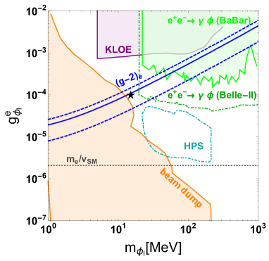
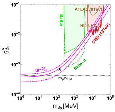
(a)	(b)

Figure 1: The color shaded regions with solid boundary are excluded by current experiments, the regions with dot-dashed boundaries are future projections. The black star corresponds to the benchmark in Table. 2. (a): The parameter space $(g_{\phi_{I}}^{e},m_{\phi_{I}})$ for $\Delta a_{e}$ and the constraints from different experiments. The shaded orange region is from beam dump experiment Batell:2016ove ; Liu:2016qwd and the dot-dashed dark cyan contour area is from future projection for HPS Battaglieri:2014hga ; Batell:2016ove . The collider limits include shaded green region searching for $e^{+}e^{-}\to\gamma\phi$ at BaBar Knapen:2017xzo , shaded purple region from KLOE Anastasi:2015qla ; Alves:2017avw and Belle-II projection Abe:2010gxa ; Batell:2016ove which is shown in dot-dashed green contour region. (b): The parameter space $(g_{\phi_{R}}^{\mu},\leavevmode\nobreak\ m_{\phi_{R}})$ for $\Delta a_{\mu}$ and the constraints from collider searches. BaBar search via $e^{+}e^{-}\to\mu^{+}\mu^{-}\phi$ is shown in the shaded green region Batell:2016ove ; Batell:2017kty and future projection for Belle-II Batell:2017kty is shown by the green dot-dashed contour. The ATLAS experiment has looked for exotic Z decay $Z\to 4\mu$ at LHC Run-I, which has been re-casted for scalar mediator by Ref. Batell:2017kty , and the limits for both Run-I and HL-LHC are shown by shaded brown region and dot-dashed brown contour. The CMS collaboration has studied a similar process at 13 TeV with an integrated luminosity of $77.3\leavevmode\nobreak\ {\rm fb}^{-1}$ , but required a dilepton resonance from two opposite-sign muons Sirunyan:2018nnz , which leads to the exclusion of the red shaded region.

III EFT model with a light complex scalar

In this section, we demonstrate at the effective field theory (EFT) level that a complex scalar $\phi$, accompanied with some symmetry assumption can simultaneously solve the $\Delta a_{e}$ and $\Delta a_{\mu}$ anomalies. The gauge charge of $\phi$ and the global $U(1)_{\rm PQ}^{e}$ charges are presented in Table. 1.

filed	$SU(2)_{L}$	$U(1)_{Y}$	$U(1)_{\rm PQ}^{e}$
$H$	2	$\frac{1}{2}$	0
$\phi$	1	0	-2
$L_{e}$	2	$\frac{1}{2}$	1
$e_{R}$	1	-1	-1

Table 1: All particles with $SU(2)_{L}\times U(1)_{Y}\times U(1)_{\rm PQ}^{e}$ charge specified, where $U(1)_{\rm PQ}^{e}$ is a global Peccei-Quinn-like symmetry. $H$ and $L_{e}$ ($e_{R}$) are SM Higgs and left-handed (right-handed) electron, while $\phi$ is the new light singlet complex scalar.

Given the particle content and charge in Table. 1, we can write down the effective theory Lagrangian as

$$\mathcal{L}_{\rm EFT}=\frac{\phi^{*}}{\Lambda_{e}}\bar{L}_{e}He_{R}+y_{\mu}\bar{L}_{\mu}H\mu_{R}+\frac{\phi^{*}\phi}{\Lambda_{\mu}^{2}}\bar{L}_{\mu}H\mu_{R}+H.c.,$$ (5)

where $\Lambda_{e,\mu}$ are interaction scales, $H$ is the SM Higgs, $L_{e,\mu}$ are SM left-handed doublets for leptons and $e_{R},\leavevmode\nobreak\ \mu_{R}$ are the right-handed SM leptons. In principle, the tau leptons could also appear in the last two terms in Eq. (5), thus flavor violation coupling can be generated. We postpone the discussion of this issue to section V. Both the SM Higgs and the new scalar $\phi$ can get vacuum expectation values (vevs),

$$H=\frac{1}{\sqrt{2}}\left(v+h+iG^{0}\right),\quad\phi=\frac{1}{\sqrt{2}}\left(v_{\phi}+\phi_{R}+i\phi_{I}\right).$$ (6)

For the electron, its mass can only come from the first term which is a dimension 5 operator, while the muon mass can come from the second and third term. It is straight forward to obtain the following relations

$$m_{e}=\frac{vv_{\phi}}{2\Lambda_{e}},\quad m_{\mu}=\frac{y_{\mu}v}{\sqrt{2}}+\frac{vv_{\phi}^{2}}{2\sqrt{2}\Lambda_{\mu}^{2}},$$ (7)

$$g_{\phi_{R}}^{e,{\rm EFT}}=-g_{\phi_{I}}^{e,{\rm EFT}}=\frac{v}{2\Lambda_{e}}=\frac{m_{e}}{v_{\phi}},\quad g_{\phi_{R}}^{\mu,{\rm EFT}}=\frac{v_{\phi}v}{\sqrt{2}\Lambda_{\mu}^{2}}.$$ (8)

We find that the CP-odd $\phi_{I}$ and CP-even scalars $\phi_{R}$ couples to electron with the same strength. For the electron anomalous magnetic dipole, the contributions from the two scalars have opposite signs. To obtain negative $\Delta a_{e}$, the $\phi_{I}$ contribution has to be larger than the $\phi_{R}$ one, which can be satisfied by requiring $m_{\phi_{I}}\ll m_{\phi_{R}}$. We emphasize that such requirement is natural to achieve, because if $U(1)_{\rm PQ}^{e}$ is spontaneously broken, the Goldstone $\phi_{I}$ is massless. However, we have to downgrade the continuous global symmetry to a discrete one, for example, adding a soft breaking term, e.g. $\mu_{4}^{2}\phi_{I}^{2}$ term to give mass to $\phi_{I}$. It can also get mass from hidden confinement scale Marques-Tavares:2018cwm . The mass of $\phi_{R}$ is not dictated by symmetry breaking, thus can be larger.

In the EFT model, we have 6 free parameters, $\Lambda_{e}$, $\Lambda_{\mu}$, $y_{\mu}$, $v_{\phi}$, $m_{\phi_{I}}$ and $m_{\phi_{R}}$. With the electron and muon masses, we can eliminate $\Lambda_{e}$ and $y_{\mu}$. To fit the anomalous magnetic moment $\Delta a_{e}$, we further eliminate $v_{\phi}$. From the electron sector, only $m_{\phi_{I}}$ is a free parameter, though is limited to a small range $10-100$ MeV from the constraints in Fig. 1 (a). We choose $m_{\phi_{I}}\sim 15$ MeV as our benchmark, which also implies $g_{\phi_{I}}^{e}\sim 10^{-4}$. Let us stress that for $\Delta a_{e}$, the 1-loop PhysRevLett.65.21 correction is suppressed by the electron mass, and hence the 2-loop Barr-Zee diagram could be dominant if $\phi_{I}$ couples to other heavy charged fermions Giudice:2012ms ; Davoudiasl:2018fbb . In our case, however, the $\phi_{I}$ only couples to the electron due to the PQ charge assignment and thus the 2-loop contribution is much smaller than the 1-loop one TuckerSmith:2010ra .

The $\Delta a_{\mu}$ defines a band in $\Lambda_{\mu}$ and $m_{\phi_{R}}$ region as well. As a result, after applying two lepton mass and $\Delta a_{e/\mu}$ requirements, we are left with 2 degree of freedom (d.o.f.) as $m_{\phi_{I}}$ and $m_{\phi_{R}}$. We list a benchmark point with $m_{\phi_{R}}\sim 15$ MeV and $m_{\phi_{R}}\sim 0.15$ GeV as an example in Table. 2. In Fig. 2, we show the fits for $\Delta a_{e/\mu}$ anomalies with the parameters $v_{\phi}$, $m_{\phi_{I}}$, $m_{\phi_{R}}$, and $\Lambda_{\mu}$.

$v_{\phi}$ (GeV)	$m_{\phi_{I}}$ (MeV)	$\Lambda_{e}$ (GeV)	$\Lambda_{\mu}$ (GeV)	$m_{\phi_{R}}$ (GeV )
$4.7$	15	$1.12\times 10^{6}$	$1080$	0.15

Table 2: The benchmark for EFT model. The parameter $y_{\mu}$ is determined by muon mass which is not listed here. The EFT model has 2 d.o.f., $m_{\phi_{I}}$ and $m_{\phi_{R}}$, after applying all the constraints and signal requirements. The change of $m_{\phi_{R}}$ only affects $\Lambda_{\mu}$, while $v_{\phi}$ and $\Lambda_{e}$ are already fixed by the electron mass and $\Delta a_{e}$. $m_{\phi_{I}}$ is limited to a small range $10-100$ MeV by relevant constraints. This benchmark is labeled as a black star in Fig. 1.

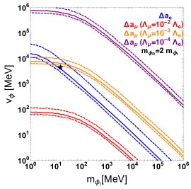
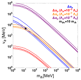
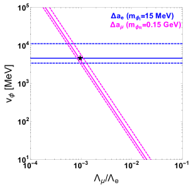
Figure 2: The EFT parameter space with parameters $v_{\phi}$, $m_{\phi_{I}}$, $m_{\phi_{R}}$, and $\Lambda_{\mu}$ for $\Delta a_{e/\mu}$ anomalies.

In the EFT model, we further consider the possibility that the muon mass comes from the dimension 6 operator, e.g. when $y_{\mu}=0$. In this case, $\Lambda_{\mu}=135$ GeV is enforced by the muon mass. It implies that $g_{\phi_{R}}^{\mu,{\rm EFT}}\approx 0.045$ and the $\phi_{R}$ mass is around $26-50$ GeV. In this case, there is no free parameter left in the EFT model. This possibility is constrained by the recent analysis of the CMS 13 TeV data with $77.3\leavevmode\nobreak\ {\rm fb}^{-1}$ Sirunyan:2018nnz shown in Fig. 1 (b), that restrict $\phi_{R}$ masses smaller than 38.5 GeV is excluded. Although masses of the order of 40 GeV would be allowed, leading to values of $a_{\mu}$ which deviate by less than 1 $\sigma$ from the experimental value, one more issue with this region of parameters is that $\Lambda_{\mu}$ is around 135 GeV, which implies new physics should be much lighter than in the original benchmark. We leave the exploration of this parameter space for future work.

IV UV complete model with a light complex scalar

In this section, we show the UV completion of the EFT Lagrangian in Eq. (5). The particle content of the UV model is listed in Table 3. It contains three Higgs doublet $\Phi_{1,2,3}$, where $\Phi_{2}$ will become the SM-like Higgs. A SM singlet complex scalar $\phi$ transforms under an approximate $U(1)$ PQ-like symmetry, while $\Phi_{1}$, $L_{e}$ and $e_{R}$ also transform under it. The symmetry has to be softly broken to allow a massive $\phi_{I}$. $\Phi_{2,3}$ have no global charge assigned.

filed	$SU(2)_{L}$	$U(1)_{Y}$	$U(1)_{\rm PQ}^{e}$
$\Phi_{1}$	2	$\frac{1}{2}$	2
$\Phi_{2}$	2	$\frac{1}{2}$	0
$\Phi_{3}$	2	$\frac{1}{2}$	0
$\phi$	1	0	-2
$L_{e}$	2	$\frac{1}{2}$	1
$e_{R}$	1	$-1$	-1

Table 3: The particles under $SU(2)_{L}\times U(1)_{Y}\times U(1)_{\rm PQ}^{e}$ , where $U(1)_{\rm PQ}^{e}$ is a global Peccei-Quinn-like symmetry. The Higgs doublet $\Phi_{1}$ and $\Phi_{3}$ are supposed to be heavy degrees of freedom, which are integrated out in the effective theory. The mixing between the scalars are assumed to be small and $\Phi_{2}$ will be the SM-like Higgs.

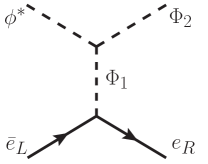
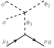
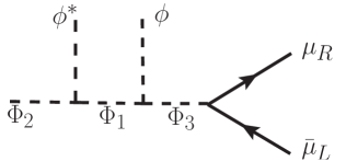
(a)	(b)	(c)

Figure 3: The relevant Feynman diagrams for generating EFT Lagrangian. The figure (a) is responsible for $\phi^{*}\bar{L}_{e}He_{R}+H.c.$, while (b) and (c) are responsible for $\phi^{*}\phi(\bar{L}_{\mu}H\mu_{R}+H.c.)$.

IV.1 The electron sector

We need the Higgs doublet $\Phi_{1}$ charged under $U(1)_{\rm PQ}^{e}$ to generate the dimension 5 operator in the EFT Lagrangian which is responsible for the electron mass. The relevant Feynman diagram is shown in Fig. 3 (a), where the heavy $\Phi_{1}$ is integrated out. The relevant UV Lagrangian for the electron sector is given by,

$$\mathcal{L}_{\rm UV}^{e} =V(\Phi_{1},\Phi_{2})_{\rm 2HDM}^{U(1)}+\left(y_{e}\bar{L}_{e}\Phi_{1}e_{R}+H.c.\right)$$

$$+V(\phi)+\frac{1}{2}\mu_{4}^{2}\phi_{I}^{2}$$

$$+(\phi^{*}\phi)\left(\lambda_{5}\Phi^{\dagger}_{1}\Phi_{1}+\lambda_{6}\Phi^{\dagger}_{2}\Phi_{2}\right)+\mu_{8}\left(\Phi^{\dagger}_{1}\Phi_{2}\phi^{*}+H.c.\right).$$ (9)

After getting a vev, the neutral component in each of the Higgs doublets is

$$\Phi_{j}^{0}=\frac{1}{\sqrt{2}}\left(v_{j}+h_{j}+ia_{j}\right),$$ (10)

where we assume $v_{3}\ll v_{1}\ll v_{2}$. For further simplicity, we assume the alignment limit that $\Phi_{2}\approx H$ and the mixing angles between $\Phi_{i}$ and $\phi$ are small. We neglect $\Phi_{3}$ at this moment, since it is not necessary for generating the EFT operators in the electron sector.

In Eq. (9), the coefficients are all real, as required by CP conservation. In the first line, the scalar potential $V(\Phi_{1},\Phi_{2})_{\rm 2HDM}^{U(1)}$ Branco:2011iw is the usual two Higgs doublet model (2HDM) potential subject to the global $U(1)$ charge. The Yukawa coupling for the electron is mediated by $\Phi_{1}$ only. In the second line, the singlet scalar potential $V(\phi)$ contains the quadratic $\phi^{*}\phi$ and quartic $(\phi^{*}\phi)^{2}$ terms satisfying the global $U(1)_{\rm PQ}^{e}$ symmetry. However, we explicitly add the $\mu_{4}^{2}\phi_{I}^{2}$ term to break $U(1)_{\rm PQ}^{e}$ softly, since otherwise $\phi_{I}$ will be a massless pseudo-Goldstone boson. In the third line , the $\mu_{8}$ term is special because it contributes to the splitting of the mass for CP-odd scalars with respect to the CP-even ones. Regarding the CP-odd sector, the mass eigenstates are a heavy massive $A^{0}$, a Goldstone boson $G^{0}$ eaten by Z gauge boson and a remaining pseudo-Goldstone $\phi_{I}^{{}^{\prime}}$ for the global $U(1)_{\rm PQ}^{e}$. In the small mixing setup, the mass eigenstates $A^{0}$, $G^{0}$ and $\phi_{I}^{{}^{\prime}}$ are mostly $a_{1}$, $a_{2}$ and $\phi_{I}$, respectively.

Following Liu:2017xmc , the mass for $A^{0}$ and $\phi_{I}^{{}^{\prime}}$ and their mixing between different states are given by

$$m_{A^{0}}^{2}=-\mu_{8}v_{2}\frac{v_{1}^{2}+v_{\phi}^{2}}{\sqrt{2}v_{1}v_{\phi}},\quad m_{\phi_{I}^{{}^{\prime}}}^{2}=\mu_{4}^{2}\frac{v_{\phi}^{2}}{v_{1}^{2}+v_{\phi}^{2}},$$ (11)

$$a_{1}=\frac{v_{\phi}}{\sqrt{v_{1}^{2}+v_{\phi}^{2}}}A^{0}+\frac{v_{1}}{v}G^{0}-\frac{v_{1}}{\sqrt{v_{1}^{2}+v_{\phi}^{2}}}\phi_{I}^{{}^{\prime}}+\mathcal{O}\left(\frac{\mu_{4}^{2}}{\mu_{8}v_{2}}\right),$$ (12)

$$\phi_{I}=\frac{v_{1}}{\sqrt{v_{1}^{2}+v_{\phi}^{2}}}A^{0}+0\times G^{0}+\frac{v_{\phi}}{\sqrt{v_{1}^{2}+v_{\phi}^{2}}}\phi_{I}^{{}^{\prime}}+\mathcal{O}\left(\frac{\mu_{4}^{2}}{\mu_{8}v_{2}}\right),$$ (13)

where $v\equiv\sqrt{v_{1}^{2}+v_{2}^{2}}$ and we have taken only the leading term under assumption $v_{2}\gg v_{\phi},v_{1}$. If we further impose $v_{\phi}\gg v_{1}$, then our assumption that scalar mixing is small can be satisfied. From the mixing in the UV model, we can calculate the coupling $g_{\phi_{I}}^{e}$ that

$$g_{\phi_{I}}^{e,{\rm UV}}=-\frac{y_{e}}{\sqrt{2}}\frac{v_{1}}{\sqrt{v_{1}^{2}+v_{\phi}^{2}}}=-\frac{m_{e}}{\sqrt{v_{1}^{2}+v_{\phi}^{2}}}.$$ (14)

After integrating out $\Phi_{1}$, one can also obtain the interaction scale $\Lambda_{e}$ that

$$\frac{1}{\Lambda_{e}}=y_{e}\frac{\mu_{8}}{m_{A_{0}}^{2}}.$$ (15)

In Eq. (15), due to CP conservation, the integrated particle should be the CP-odd component in $\Phi_{1}$, thus the denominator is the mass of $A_{0}$ squared. Applying Eq. (11) and Eq. (15), one can check that $g_{\phi_{I}}^{e,{\rm EFT}}$ in Eq. (8) agrees with $g_{\phi_{I}}^{e,{\rm UV}}$. One can also see that the mass of $A^{0}$ can be easily as large as 1 TeV if $\mu_{8}$ is electroweak scale and $v_{\phi}/v_{1}$ is large.

IV.2 The muon sector

In this section, we describe the UV model which can generate the dimension 6 operator in $\mathcal{L}_{\rm EFT}$, which is responsible for the $\phi_{R}$ coupling to muons. A third Higgs doublet $\Phi_{3}$ is essential and it has to carry the same quantum charge as SM-like Higgs $\Phi_{2}$. The relevant Lagrangian is

$$\mathcal{L}_{\rm UV}^{\mu} =V(\Phi_{2},\Phi_{3})_{\rm 2HDM}+(y_{\mu}\bar{L}_{\mu}\Phi_{2}\mu_{R}+y_{\mu 3}\bar{L}_{\mu}\Phi_{3}\mu_{R}+H.c.)$$

$$+V(\phi)+(\phi^{*}\phi)\left(\lambda_{6}\Phi^{\dagger}_{2}\Phi_{2}+\lambda_{8}\Phi^{\dagger}_{3}\Phi_{3}\right)$$

$$+\lambda_{9}(\phi^{*}\phi)\left(\Phi^{\dagger}_{2}\Phi_{3}+H.c.\right)+\mu_{9}\left(\Phi^{\dagger}_{1}\Phi_{3}\phi^{*}+H.c.\right),$$ (16)

where the coefficients are real.

The first line in Eq. (16) contains a general 2HDM scalar potential $V(\Phi_{2},\Phi_{3})_{\rm 2HDM}$. The last two terms in that line are the Yukawa couplings for the muon. We will again assume hierarchical vevs, $v_{3}\ll v_{1}\ll v_{\phi}\ll v_{2}$, so that the muon mass predominantly comes from $\Phi_{2}$ and $y_{\mu 3}$ is free from the muon mass constraint. The second line contains the scalar potential for $\phi$ and the quartic coupling between $\phi$ and $\Phi_{2,3}$. Since $v_{3}\sim 0$, if we require $\lambda_{6}\ll 1$, the quartic term in the second line does not induce a large mixing between the different scalars. Since $\Phi_{2}$ and $\Phi_{3}$ have the same quantum numbers, the potential $V(\Phi_{2},\Phi_{3})_{\rm 2HDM}$ may include a quadratic term $m_{23}^{2}\Phi_{3}^{\dagger}\Phi_{2}+H.c.$, while the third line contains the term proportional to $\lambda_{9}$ which may also lead to a similar term when $\phi$ acquires a vev. These two terms contribute to the dimension 4 and 6 operators responsible for the muon mass and the coupling of $\phi_{R}$ to the muons in the effective field theory described by $\mathcal{L}_{\rm EFT}$, Eq. (5). Finally, the term proportional to the trilinear mass parameter $\mu_{9}$, in combination with the $\mu_{8}$-induced interactions, can also contribute to the $\phi_{R}$ coupling to muons. Although all these contributions may coexist, we shall treat them in a separate way for simplicity of presentation.

IV.2.1 Generating the operators from quartic scalar interactions

The term proportional to the $\lambda_{9}$ coupling in Eq. (16) can generate the Feynman diagram depicted in Fig. 3 (b), which can lead, after integrating out $\Phi_{3}$, to the coupling of $\phi_{R}$ to muons in the EFT, Eq. (5). This coupling is given by

$$g_{\phi_{R}}^{\mu,{\rm EFT}}=\frac{v_{\phi}v}{\sqrt{2}\Lambda_{\mu}^{2}}=y_{\mu 3}\lambda_{9}\frac{v_{\phi}v_{2}}{\sqrt{2}m_{h_{3}}^{2}},$$ (17)

where $m_{h_{3}}^{2}$ is the CP-even scalar mass from $\Phi_{3}$. The interaction scale $\Lambda_{\mu}$ is related to the heavy Higgs parameters by the relation

$$\frac{1}{\Lambda_{\mu}^{2}}=\frac{y_{\mu 3}\lambda_{9}}{m_{h_{3}}^{2}}.$$ (18)

Given the fact that the $\lambda_{9}$ term gives the off-diagonal mass terms between $\phi_{R}$ and $h_{3}$, we can calculate the mass matrix and obtain the mixing angle,

$$M^{2}_{\phi_{R}h_{3}}=\left(\begin{array}[]{cc}m_{\phi_{R}}^{2}&\lambda_{9}v_{\phi}v_{2}\\ \lambda_{9}v_{\phi}v_{2}&m_{h_{3}}^{2}\end{array}\right),$$ (21)

$$\sin\theta_{\phi_{R}h_{3}}\approx\lambda_{9}\frac{v_{\phi}v_{2}}{m_{h_{3}}^{2}}.$$ (22)

Assuming that $h_{3}$ and $\phi_{R}$ only have a small mixing between themselves ($\sin\theta_{\phi_{R}h_{3}}\ll 1$) and negligible mixing with other fields, the coupling between $\phi_{R}$ and the muon from the UV model is

$$g_{\phi_{R}}^{\mu,{\rm UV}}=\frac{y_{\mu 3}}{\sqrt{2}}\sin\theta_{\phi_{R}h_{3}}.$$ (23)

One can easily check that it agrees with $g_{\phi_{R}}^{\mu,{\rm EFT}}$ in Eq. (8) and Eq. (17).

In the UV model, the $\lambda_{9}$ and $\lambda_{8}$ terms in $\mathcal{L}_{\rm UV}^{\mu}$ contain only $\phi^{*}\phi$, thus $\phi_{I}$ couples to muon only in quadrature and can not contribute to $\Delta a_{\mu}$. Given that $\Lambda_{\mu}$ needs to be about $1080$ GeV (see Table 2), the scalar boson $h_{3}$ can be easily heavier than $\mathcal{O}(1)$ TeV, as can be seen from Eq. (18).

IV.2.2 Generating the operators from triplet scalar interaction

We can generate the CP-even scalar $\phi_{R}$ coupling to muon via Fig.3 (c), after integrating out the heavy $h_{1}$ and $h_{3}$ scalar bosons. As emphasized above, it requires the simultaneous action of the two triple scalar couplings $\mu_{9}\Phi^{\dagger}_{1}\Phi_{3}\phi^{*}$ and $\mu_{8}\Phi^{\dagger}_{1}\Phi_{2}\phi^{*}$. According to Liu:2017xmc , under the assumption $v_{1}\ll v_{\phi}\ll v_{2}$, $m_{h_{1}}^{2}$ is the same order as $m_{A_{0}}^{2}$ in Eq. (11), what is also confirmed in the full UV model calculation presented in Appendix A. The EFT coupling between $\phi_{R}$ and muon can be computed as

$$g_{\phi_{R}}^{\mu,{\rm EFT}}=\frac{y_{\mu 3}v_{\phi}v_{2}\mu_{8}\mu_{9}}{\sqrt{2}m_{h_{1}}^{2}m_{h_{3}}^{2}}\approx y_{\mu 3}\frac{v_{1}\mu_{9}}{m_{h_{3}}^{2}},$$ (24)

where $m_{h_{1,3}}^{2}$ are the CP-even scalar mass from $\Phi_{1,3}$. The interaction scale $\Lambda_{\mu}$ in this case is

$$\frac{1}{\Lambda_{\mu}^{2}}=\frac{y_{\mu 3}\mu_{8}\mu_{9}}{m_{h_{1}}^{2}m_{h_{3}}^{2}}.$$ (25)

In the UV model, the $\phi_{R}$ coupling to muon again comes from mixing with $h_{3}$. We calculate the mass matrix and obtain the mixing angle via $\mu_{9}\Phi^{\dagger}_{1}\Phi_{3}\phi^{*}$ term,

$$M^{2}_{\phi_{R}h_{3}}=\left(\begin{array}[]{cc}m_{\phi_{R}}^{2}&\mu_{9}v_{1}\\ \mu_{9}v_{1}&m_{h_{3}}^{2}\end{array}\right),$$ (28)

$$\sin\theta_{\phi_{R}h_{3}}\approx\frac{\mu_{9}v_{1}}{m_{h_{3}}^{2}},$$ (29)

where again we find that $g_{\phi_{R}}^{\mu,{\rm UV}}\equiv y_{\mu 3}\sin\theta_{\phi_{R}h_{3}}$ agrees with $g_{\phi_{R}}^{\mu,{\rm EFT}}$ again. In the above discussion, we did not include off-diagonal terms with $h_{1,2}$. The $\phi_{R}$-$h_{3}$ mixing, may be modified through the mixing with them. We did the full calculation in the 3HDM plus a singlet complex scalar in Appendix A. The result contains more terms than Eq. (29), but one can tune down some parameters to converge to this result, while keeping the $\Phi_{1,3}$ scalars heavy. Such tuning is also in agreement of the initial assumption that the mixing between different scalars is small, see Appendix A.

From the benchmark point, we can see that a coupling $g_{\phi_{R}}^{\mu,{\rm EFT}}\sim 0.7\times 10^{-3}$ can fit the $\Delta a_{\mu}$ anomaly. One can infer the mass square $m_{h_{3}}^{2}\simeq 10^{3}y_{\mu 3}v_{1}\mu_{9}$ from Eq. (24). With a large $\mu_{9}\simeq\mathcal{O}({\rm few})$ TeV and $v_{1}\sim 1$ GeV, $h_{3}$ mass can be larger than $\mathcal{O}(1)$ TeV.

Given the fact that the $\phi_{I}^{{}^{\prime}}$ mass is much smaller than $\phi_{R}$, any small mixing between $\phi_{I}^{{}^{\prime}}$ and the CP-odd components of $\Phi_{2}$ and $\Phi_{3}$, would induce a coupling of $\phi_{I}^{{}^{\prime}}$ to muons, that could make the contribution from $\phi_{I}^{{}^{\prime}}$ to $\Delta a_{\mu}$ larger than the one of $\phi_{R}$. However, in the full calculation within the 3HDM plus singlet scalar potential, presented in Appendix A, the mass eigenstate $\phi_{I}^{{}^{\prime}}$ only mixes with $a_{1}$ in the leading order of $v_{1}/v_{\phi}$. In fact, the absence of mixing with $a_{2,3}$ can be simply understood from the pseudo-Goldstone nature of this particle. Thus, the components of $\phi_{I}^{{}^{\prime}}$ are approximately described by Eq. (12), and $\phi_{I}^{{}^{\prime}}$ only couples to electrons, as occurs in the EFT model.

V Phenomenology constraints

There are several important phenomenological constraints to address, once moving from EFT model to the UV model.

V.1 Heavy scalars and anomalous magnetic moments

One relevant constraint is the contribution of the heavy scalars to the anomalous magnetic moments. Although these scalars are integrated out in the EFT, they may contribute in a relevant way. At large mass, the CP-even scalar contribution to the lepton g-2 is approximately given by $\Delta a_{\ell}^{\rm even}\approx g_{S\ell}^{2}/(8\pi^{2})m_{\ell}^{2}/m_{S}^{2}(\log(m_{S}^{2}/m_{\ell}^{2})-7/6)$, while CP-odd scalar contributes as $\Delta a_{\ell}^{\rm odd}\approx g_{S\ell}^{2}/(8\pi^{2})m_{\ell}^{2}/m_{S}^{2}(-\log(m_{S}^{2}/m_{\ell}^{2})+11/6)$ Giudice:2012ms . Neglecting the mild dependence on log terms, the anomalous magnetic moments are hence proportional to $g_{\ell}^{2}/m_{S}^{2}$.

In the UV model, the light scalar couples to leptons via mixing with the heavy ones for the pseudo-scalar case, where the mixing angles are related to vevs due to pseudo-Goldstone nature. Therefore, for light scalar contribution dominating over the heavy scalar one, the relation $\sin^{2}\theta>m_{\rm light}^{2}/m_{\rm heavy}^{2}$ must be satisfied, where $\sin\theta$ is the mixing angle, while $m_{\rm light}$ and $m_{\rm heavy}$ are the light and heavy scalar masses. The mixing angles do not significantly depend on the mass of the light scalars, $m_{\rm light}$, thus one can always tune down light scalar mass to meet the requirement. It is easy to find that the $a_{1}$ contributions to the $e$ anomalous magnetic moments is sub-dominant than the $\phi_{I}$ ones due to the small values of the lightest pseudo-scalar mass, while satisfying the benchmark requirements.

However, for CP-even scalar $h_{3}$ mixing, the mixing angle $\sin\theta$ is proportional to $m_{h_{3}}^{-2}$. Therefore, $\sin^{2}\theta\propto m_{h_{3}}^{-4}$ and the $\sin^{2}\theta>m_{\rm light}^{2}/m_{\rm heavy}^{2}$ condition actually provides an upper bound on the $h_{3}$ mass. If we choose the benchmark presented in Table 2, with $v_{\phi}=4.7$ GeV, $m_{\phi_{R}}=0.15$ GeV, and $g_{\phi_{R}}^{\mu,\text{EFT}}=0.7\times 10^{-3}$, for the cases in which the effective low energy couplings are induced by quartic (triplet) scalar interactions, the $h_{3}$ contribution would be smaller than $\phi_{R}$ provided that

$$m_{h_{3}}<\lambda_{9}\times 7.7\leavevmode\nobreak\ {\rm TeV}\leavevmode\nobreak\ \;(m_{h_{3}}<6.7\times\mu_{9}v_{1}\text{GeV}^{-1}).$$ (30)

To satisfy $g_{\phi_{R}}^{\mu,\text{EFT}}=0.7\times 10^{-3}$, for quartic (triplet) scalar interactions, one should further demand that $m_{h_{3}}=1\leavevmode\nobreak\ \text{TeV}\times\sqrt{\lambda_{9}y_{\mu 3}}$ ($m_{h_{3}}=37.8\sqrt{y_{\mu 3}\mu_{9}v_{1}}$), as can be seen from Eqs. (17) and (24). These requirements can be achieved easily, with $\lambda_{9}\sim 1$ and $y_{\mu 3}\sim 1$ for quartic case, while $\mu_{9}\sim 1$ TeV, $v_{1}\sim 1$ GeV and $y_{\mu 3}\sim 1$ for triplet case. It is worth mentioning that $m_{h_{3}}$ is about 1 TeV in both cases. Therefore, we conclude that in the UV model, under the hierarchical vevs and heavy $\Phi_{1,3}$ assumptions, the heavy scalars do not contribute to the anomalous magnetic moment in a relevant way.

Moreover, we comment that the way of generating dimension 6 operators in the EFT model is not restricted to those ones depicted in Fig. 3 (b) and (c). Since $\Phi_{2,3}$ have the same quantum number, the scalar potential $V(\Phi_{2},\Phi_{3})_{\rm 2HDM}$ interactions are only weakly constrained and could induce large $h_{2}$-$h_{3}$ mixing. As discussed in Appendix A, and emphasized before, in the presence of large $\lambda_{6}$ or $\mu_{8}$ terms, these mixing effects can lead to large contributions to the dimension 6 operator in the EFT model. Let us stress, however, that large $\lambda_{6}$ and $\mu_{8}$ terms can also induce large mixing between $h_{2}$-$\phi_{R}$. Such possibility beyond the scope of the EFT model and is in tension with our initial assumption that mixing between different scalars are all small.

V.2 Scalar interactions and relevant phenomenology

The next constraint is the decay channels modified by scalar interactions. In the EFT model, $\phi_{I}$ decays to $e^{+}e^{-}$, while $\phi_{R}$ decays to $e^{+}e^{-}$ with same coupling as $\phi_{I}$. $\phi_{R}$ can also decay to $\mu^{+}\mu^{-}$ if kinematics allowed. With the scalar potential from UV model, e.g. 3HDM plus singlet scalar in Appendix A, there are a few phenomenologically relevant decay channels, $\phi_{R}^{{}^{\prime}}\to\phi_{I}^{{}^{\prime}}\phi_{I}^{{}^{\prime}}$, $H_{2}^{0}\to\phi_{I}^{{}^{\prime}}\phi_{I}^{{}^{\prime}}$ and $H_{2}^{0}\to\phi_{R}^{{}^{\prime}}\phi_{R}^{{}^{\prime}}$, where $\phi_{I,R}^{{}^{\prime}}$ and $H_{2}^{0}$ are mass eigenstates of CP-even (CP-odd) light scalars and SM Higgs. According to the mixing matrix for both CP-even (odd) scalars in Appendix A, the triple scalar couplings between the mass eigenstates $\phi_{I,R}^{{}^{\prime}}$ and $H_{2}^{0}$ can be calculated,

$$\mathcal{L}_{\rm tri}=\left(\lambda_{\phi}-\lambda_{6}\left(\frac{\lambda_{6}}{4\lambda_{2}}+\frac{\mu_{8}v_{1}}{\sqrt{2}\lambda_{2}v_{2}v_{\phi}}\right)\right)v_{\phi}\phi^{{}^{\prime}2}_{I}\phi^{{}^{\prime}}_{R}+\left(\frac{\lambda_{6}}{2}+\frac{\mu_{8}v_{1}}{\sqrt{2}v_{2}v_{\phi}}\right)v_{2}\left(\phi^{{}^{\prime}2}_{I}H_{2}^{0}+\phi^{{}^{\prime}2}_{R}H_{2}^{0}\right).$$ (31)

First, from our benchmark, we have $v_{\phi}=4.7$ GeV, $m_{\phi_{I}^{{}^{\prime}}}\approx 15$ MeV and $v_{1}\ll v_{\phi}$. The CP-even scalar $\phi_{R}^{{}^{\prime}}$ has a coupling which is about $10^{-4}(10^{-3})$ to electrons (muons) respectively, while its coupling to pairs of $\phi_{I}^{{}^{\prime}}$ is $2\lambda_{\phi}v_{\phi}$. Thus, $\phi_{R}^{{}^{\prime}}$ will dominantly decay into $\phi_{I}^{{}^{\prime}}$ pairs. Assuming $m_{\phi_{R}^{{}^{\prime}}}\sim\sqrt{\lambda_{\phi}}v_{\phi}$, the branching ratio of its decay into $e^{-}e^{+}$ ($\mu^{+}\mu^{-}$) will be about $\sim 10^{-8}$ ($10^{-6}$) respectively. Then, the previous constraints on $\phi_{R}^{{}^{\prime}}$ shown in Fig. 1 (b), which are based on the assumption $BR(\phi_{R}^{{}^{\prime}}\to\ell^{+}\ell^{-})\sim 1$, should be revised. At low energy electron colliders, the relevant search channels are $e^{+}e^{-}\to\gamma\phi^{\prime}_{R}$ and $e^{+}e^{-}\to\phi_{R}^{{}^{\prime}*}\to\phi^{\prime}_{I}\phi^{\prime}_{I}$, governed by the electron coupling and $e^{+}e^{-}\to\mu^{+}\mu^{-}\phi^{\prime}_{R}$ governed by the muon coupling. Since $\phi^{\prime}_{R}\to\phi^{\prime}_{I}\phi^{\prime}_{I}\to 4e$, there are multiple leptons in the final state. Although the BaBar experiment has searched for new physics in similar channels, for instance $e^{+}e^{-}\to h^{\prime}A^{\prime}$, $h^{\prime}\to A^{\prime}A^{\prime}$ and $A^{\prime}\to\ell^{+}\ell^{-}$ Lees:2012ra and $e^{+}e^{-}\to W^{\prime}W^{\prime}\to 2(\ell^{+}\ell^{-})$ in exclusive mode Aubert:2009af , it has not explored the invariant mass regions consistent with $m_{\phi_{I}^{{}^{\prime}}}$. However, BaBar has the capability of lowering the invariant mass threshold, as has been shown in the 2014 search for dark photons via $\gamma A^{\prime}$ channel Lees:2014xha , where the BaBar collaboration extended the di-electron resonance channel to $m_{e^{+}e^{-}}>0.015$ GeV, and fits for $m_{A^{\prime}}>0.02$ GeV. We believe it would be important to reanalyze their searches by imposing similar bounds on the dielectron invariant mass. Moreover, since $\phi_{I}^{{}^{\prime}}$ and $\phi_{R}^{{}^{\prime}}$ are pretty light, they will be very boosted at high energy colliders and form lepton jets ArkaniHamed:2008qp ; Baumgart:2009tn ; Bai:2009it ; Katz:2009qq . The proper lifetime of $\phi_{I}^{{}^{\prime}}$ in the benchmark is about $c\tau\approx 10^{-3}{\rm cm}$, thus it will appear as a prompt lepton jet in a low energy lepton collider, but displaced lepton jet at the LHC. The displacement could help the search at the LHC, to separate the signal from the SM background, for example photon conversions. However, the invariant mass of the di-electron or even four lepton events coming from $\phi_{R}^{{}^{\prime}}$ might be too low for the LHC experiments to detect them.

Second, we discuss the exotic SM Higgs decay channels $H_{2}^{0}\to\phi_{I}^{{}^{\prime}}\phi_{I}^{{}^{\prime}}\to 2(e^{+}e^{-})$ and $H_{2}^{0}\to\phi_{R}^{{}^{\prime}}\phi_{R}^{{}^{\prime}}\to 4(e^{+}e^{-})$. It is clear that if $\lambda_{6}$ is of $\mathcal{O}(1)$, then the SM-like Higgs will dominantly decay to those light scalars thus one needs $\lambda_{6}\ll 1$. The ratio $\mu_{8}v_{1}/(\sqrt{2}v_{2}v_{\phi})$ should also be small. To obtain a $H_{2}^{0}\to\phi_{I}^{{}^{\prime}}\phi_{I}^{{}^{\prime}},\phi_{R}^{{}^{\prime}}\phi_{R}^{{}^{\prime}}$ branching ratio smaller than $1\%$, the coefficient $\lambda_{6}$ or $\mu_{8}v_{1}/(\sqrt{2}v_{2}v_{\phi})$ should be $\lesssim 10^{-3}$, thus $\mu_{8}v_{1}\lesssim 1.7\leavevmode\nobreak\ {\rm GeV}^{2}$. If we tune down both $\mu_{8}$ and $v_{1}$, the $A_{1}^{0}/H_{1}^{0}$ masses, of about $\sqrt{v_{\phi}v_{2}(\mu_{8}/v_{1})}$ (see Appendix A), can still remain as heavy as $\sim 300$ GeV, with $\mu_{8}\sim 10$ GeV and $v_{1}\sim 0.1$ GeV. Interestingly, in the electron sector, we have $m_{e}=y_{e}v_{1}/\sqrt{2}$, which suggests $v_{1}\gtrsim m_{e}$ and one can further decrease $v_{1}$ to make $A_{1}^{0}/H_{1}^{0}$ heavier. Furthermore, according to Eq. (14), the coupling $g_{\phi_{I}}^{e}$ is not affected by a small $v_{1}$. One should note that, as we mentioned before, in the case $g_{\phi_{R}}^{\mu}$ is generated from triplet scalar interactions, we have from Eq. (24) that for the benchmark presented in Table 2, $m_{h_{3}}=37.8\sqrt{y_{\mu 3}\mu_{9}v_{1}}$. Hence, if we take $v_{1}=0.1$ GeV while keeping $\mu_{9}\sim 1$ TeV and $y_{\mu 3}\sim 1$, the mass $m_{h_{3}}$ goes down to $\sim 380$ GeV and will become smaller for smaller values of $v_{1}$. However, for the case $g_{\phi_{R}}^{\mu}$ is generated from quartic scalar interaction, Eqs. (17), the mass $m_{h_{3}}$ does not have a strong dependence on $v_{1}$ and hence could remain heavy even for very small values of $v_{1}$.

V.3 Charged lepton flavor violation

In this section, we discuss the possible flavor changing neutral current (FCNC) constraint. Since the muon and the tau leptons have the same quantum number, in the EFT Lagrangian, Eq. (5), the muon leptons can be substituted with tau leptons. Moreover, in the UV model, the two Higgs doublets $\Phi_{2,3}$ have the same quantum charge and hence admit the same couplings. After the charged lepton mass matrix diagonalization, a possible misalignment between the lepton mass and Yukawa couplings can induce off-diagonal Yukawa couplings to muons and taus, see also a recent review Lindner:2016bgg on $\Delta a_{\mu}$ and lepton flavor violation. To avoid the appearance of FCNC, one can assume minimal flavor violation (MFV) Chivukula:1987py ; DAmbrosio:2002vsn to align the couplings of $\Phi_{3}$ with the $\Phi_{2}$ ones. In the case of MFV, $\Phi_{3}$ will also couple to muon and tau lepton with diagonal couplings weighted by the lepton masses. Heavy Higgs bosons, which couple only to leptons and gauge bosons are difficult to test at hadron colliders. Under the MFV assumption, however, the light scalar $\phi_{R}^{{}^{\prime}}$ couples in a relevant way to $\tau$ leptons and is constrained to have a mass between $30-200$ MeV in order to be consistent with precision electroweak constraints associated with loop corrections to $Z\to\tau^{+}\tau^{-}$ Abu-Ajamieh:2018ciu .

While MFV can solve the FCNC constraint for heavy scalars, the constraints on the light scalar couplings remain severe. This is represented by the LFV decay $\tau\to\mu\phi^{\prime}_{R}\to\mu+2(e^{+}e^{-})$. The total width of $\tau$ is very small, $2.27\times 10^{-12}$ GeV and the current limit on the three lepton LFV decay is ${\rm BR}(\tau\to\mu e^{+}e^{-})<1.8\times 10^{-8}$ Tanabashi:2018oca . This limit is easy to satisfy because ${\rm BR}(\tau\to\mu e^{+}e^{-})={\rm BR}(\tau\to\mu\phi^{\prime}_{R})\times{\rm BR}(\phi^{\prime}_{R}\to e^{+}e^{-})$ for our benchmark point and ${\rm BR}(\phi^{\prime}_{R}\to e^{+}e^{-})\sim 10^{-8}$ as discussed above. However, since $\phi_{R}^{\prime}$ can decay into pairs of $\phi_{I}^{\prime}$, there is a potential flavor violation in the channel $\tau\to\mu+2(e^{+}e^{-})$. We did not find limits on this channel at the PDG Tanabashi:2018oca , but if the limits were of the same order as the one on ${\rm BR}(\tau\to\mu e^{+}e^{-})$, it will imply $y_{\tau\mu}^{\phi_{R}}\lesssim 10^{-10}$. Since $y_{\tau\mu}^{\phi_{R}}=\sin\theta_{\phi_{R}h_{3}}y_{\tau\mu}^{h_{3}}$, and the mixing angle is about $10^{-3}$, one should restrict the LFV coupling $y_{\tau\mu}^{h_{3}}$ down to $10^{-7}$. Therefore, the alignment of the lepton Yukawa couplings must be enforced by a symmetry. The most natural candidate would be an extra global $U(1)_{\mu}\times U(1)_{\tau}$ symmetry, which is vector-like when applied to fermions unlike the chiral $U(1)_{\rm PQ}^{e}$. These symmetries forbid the off-diagonal terms between charged lepton species, and then the charged lepton mass matrix is diagonal and LFV is not present in the charged lepton sector.

V.4 Others constraints and discussion

Besides the FCNC issue, the Pontecorvo–Maki–Nakagawa–Sakata (PMNS) matrix for the lepton sector needs to be generated. Given the global $U(1)_{\rm PQ}^{e}\times U(1)_{\mu}\times U(1)_{\tau}$ symmetry, the Yukawa matrices of the SM charged and neutral leptons are diagonal. However, assuming a see-saw mechanism, one can generate the PMNS matrix from mixing in the heavy sterile neutrino sector Pascoli:2006ci ; King:2013eh ; Akhmedov:2013hec , by assuming that the mass terms of the sterile neutrino $m^{N}_{ij}N^{c}_{i}N_{j}$ softly break the global symmetry (see, for instance, the review, Ref. Xing:2015fdg , for the case of $U(1)_{\mu-\tau}$).

Finally, we briefly mention that a $\phi^{\prime}_{I}$ mass around 15 MeV, as required to satisfy $\Delta a_{e}$ and the other relevant phenomenological constraints, is accidentally within the mass region necessary to explain the so-called ^8Be^* anomaly, observed by the Atomki collaboration Krasznahorkay:2015iga . Addressing this anomaly would imply a coupling of the singlet scalar to quarks, something that is beyond the scope of our work. Let us stress, however, that the authors of Ref. Ellwanger:2016wfe ; Alves:2017avw concluded that this possibility is subject to relevant constraints from low energy meson experiments that can only be avoided by assuming specific coupling structures in the quark sector.

VI Conclusions

We have presented a scenario with a light complex scalar which can simultaneously accommodate the anomalies in the electron and muon anomalous magnetic moments. The interesting feature is that the same complex scalar induces positive contributions to $a_{\mu}$ and negative contributions to $a_{e}$. This is achieved by assuming that the CP-even component is much heavier than the CP-odd component and having the CP-odd scalar scalar coupled only to electrons, while the CP-even couples to both the electron and muon fields. This scenario may be realized in a natural way by introducing an approximate PQ-like symmetry and assuming that the CP-odd scalar is a pseudo-Goldstone boson associated to its spontaneous breakdown. The EFT model can then be written down directly and cope with the anomalies, while evading all the existing constraints.

We also analyzed how to generate such EFT model from a Standard Model extension containing multiple Higgs doublets. While the additional heavy Higgs doublet masses may be as large as 1 TeV, flavor changing neutral currents may be avoided by assuming a global symmetry in the lepton sector, broken softly in the neutrino sector. Furthermore, the heavy scalars contribution to the anomalous magnetic moments is much smaller than the one of the light scalars due to the small masses of the CP-odd and even component of the complex scalar compared to the ones of the heavy Higgs bosons. For the light complex scalar, its CP-odd and even components could be potentially reached by future B-factories and the HL-LHC. Looking for multiple prompt lepton jets in low energy electron collider and displaced lepton jets from exotic SM Higgs decay at LHC is also a promising way to find those light scalars.

Appendix A The CP-even and CP-odd scalars in full UV model

We consider the full UV model with three Higgs doublet $\Phi_{1,2,3}$ and one singlet complex scalar $\phi$, where $\Phi_{1}$ and $\phi$ carries global $U(1)_{PQ}^{e}$ charge. The general scalar potential is

$$V= \mu_{1}^{2}\Phi_{1}^{\dagger}\Phi_{1}+\mu_{2}^{2}\Phi_{2}^{\dagger}\Phi_{2}+\mu_{3}^{2}\Phi_{3}^{\dagger}\Phi_{3}+\mu_{\phi}^{2}\phi^{*}\phi-m_{23}^{2}\left(\Phi_{2}^{\dagger}\Phi_{3}+\Phi_{3}^{\dagger}\Phi_{2}\right)+\frac{1}{2}\mu_{4}^{2}\phi_{I}^{2}$$

$$+\lambda_{1}\left(\Phi_{1}^{\dagger}\Phi_{1}\right)^{2}+\lambda_{2}\left(\Phi_{2}^{\dagger}\Phi_{2}\right)^{2}+\lambda_{3}\left(\Phi_{3}^{\dagger}\Phi_{3}\right)^{2}+\lambda_{\phi}\left(\phi^{*}\phi\right)^{2}+\lambda_{4}\left(\Phi_{1}^{\dagger}\Phi_{1}\right)\left(\Phi_{2}^{\dagger}\Phi_{2}\right)$$

$$+\lambda_{5}\left(\Phi_{1}^{\dagger}\Phi_{1}\right)\left(\phi^{*}\phi\right)+\lambda_{6}\left(\Phi_{2}^{\dagger}\Phi_{2}\right)\left(\phi^{*}\phi\right)+\lambda_{7}\left(\Phi_{2}^{\dagger}\Phi_{1}\right)\left(\Phi_{1}^{\dagger}\Phi_{2}\right)+\lambda_{8}\left(\Phi_{3}^{\dagger}\Phi_{3}\right)\left(\phi^{*}\phi\right)$$

$$+\lambda_{9}\left(\Phi_{2}^{\dagger}\Phi_{3}+\Phi_{3}^{\dagger}\Phi_{2}\right)\left(\phi^{*}\phi\right)+\mu_{8}\left(\Phi_{1}^{\dagger}\Phi_{2}\phi^{*}+H.c.\right)+\mu_{9}\left(\Phi_{1}^{\dagger}\Phi_{3}\phi^{*}+H.c.\right)$$

$$+\lambda_{23}^{a}\left(\Phi_{2}^{\dagger}\Phi_{2}\right)\left(\Phi_{3}^{\dagger}\Phi_{3}\right)+\lambda_{23}^{b}\left(\Phi_{2}^{\dagger}\Phi_{3}\right)\left(\Phi_{3}^{\dagger}\Phi_{2}\right)$$

$$+\lambda_{23}^{c}\left[\left(\Phi_{2}^{\dagger}\Phi_{3}\right)^{2}+\left(\Phi_{3}^{\dagger}\Phi_{2}\right)^{2}\right]+\left(\lambda_{23}^{d}\Phi_{2}^{\dagger}\Phi_{2}+\lambda_{23}^{e}\Phi_{3}^{\dagger}\Phi_{3}\right)\left(\Phi_{2}^{\dagger}\Phi_{3}+\Phi_{3}^{\dagger}\Phi_{2}\right)+\ldots$$ (32)

where we only written the scalar potential contributions, Eq. (9) and Eq. (16), which are relevant to the computation of $\Delta a_{e,\mu}$. The “$\ldots$” denotes the irrelevant terms like $(\Phi_{1}^{\dagger}\Phi_{1})(\Phi_{3}^{\dagger}\Phi_{3})$ etc, which are neglected to avoid a too cumbersome computation.

Minimizing the scalar potential, one obtains the following relations

$$\mu_{1}^{2}= -\left[\lambda_{1}v_{1}^{2}+\frac{\left(\lambda_{4}+\lambda_{7}\right)}{2}v_{2}^{2}+\frac{\lambda_{5}}{2}v_{\phi}^{2}+\frac{v_{\phi}}{\sqrt{2}v_{1}}\left(\mu_{8}v_{2}+\mu_{9}v_{3}\right)\right],$$

$$\mu_{2}^{2}= -\left[\lambda_{2}v_{2}^{2}+\frac{\lambda_{23}^{a}+\lambda_{23}^{b}+2\lambda_{23}^{c}}{2}v_{3}^{2}+\frac{\left(\lambda_{4}+\lambda_{7}\right)v_{1}^{2}}{2}+\frac{\lambda_{6}v_{\phi}^{2}}{2}\right.$$

$$\left.+\frac{v_{3}}{2v_{2}}\left(3\lambda_{23}^{d}v_{2}^{2}+\lambda_{23}^{e}v_{3}^{2}+\lambda_{9}v_{\phi}^{2}-2m_{23}^{2}\right)+\frac{\mu_{8}v_{1}v_{\phi}}{\sqrt{2}v_{2}}\right],$$

$$\mu_{3}^{2}= -\left[\lambda_{3}v_{3}^{2}+\frac{\lambda_{23}^{a}+\lambda_{23}^{b}+2\lambda_{23}^{c}}{2}v_{2}^{2}+\frac{v_{2}}{2v_{3}}\left(\lambda_{23}^{d}v_{2}^{2}+3\lambda_{23}^{e}v_{3}^{2}-2m_{23}^{2}\right)+\frac{v^{2}_{\phi}}{2v_{3}}\left(\lambda_{8}v_{3}+\lambda_{9}v_{2}\right)+\frac{\mu_{9}v_{1}v_{\phi}}{\sqrt{2}v_{3}}\right],$$

$$\mu_{\phi}^{2}= -\left[\lambda_{\phi}v_{\phi}^{2}+\frac{\lambda_{5}v_{1}^{2}+\lambda_{6}v_{2}^{2}+\lambda_{8}v_{3}^{2}+2\lambda_{9}v_{2}v_{3}}{2}+\frac{v_{1}}{\sqrt{2}v_{\phi}}\left(\mu_{8}v_{2}+\mu_{9}v_{3}\right)\right].$$ (33)

We can diagonalize the mass matrix of CP-even or CP-odd scalars and obtain the mass in the leading order under the assumption $v_{3}\ll v_{1}\ll v_{\phi}\ll v_{2}$ and $v_{2}\sim\mu_{8,9}\sim m_{23}$. The results for the CP-odd scalars are given by the eigenvalues

$$m_{A^{0}_{1}}^{2} \approx-\frac{v_{\Phi}}{\sqrt{2}v_{1}}\left(\mu_{8}v_{2}+\mu_{9}v_{3}\right),$$ (34)

$$m_{A^{0}_{3}}^{2} \approx\frac{v_{2}\left(2m_{23}^{2}-\lambda_{23}^{d}v_{2}^{2}-\lambda_{9}v_{\phi}^{2}\right)-\sqrt{2}\mu_{9}v_{1}v_{\phi}}{2v_{3}}-2\lambda_{23}^{c}v_{2}^{2},$$ (35)

$$m_{\phi^{\prime}_{I}}^{2} \approx\mu_{4}^{2},$$ (36)

where $A^{0}_{2}$ is the massless Goldstone associated with the breakdown of the electroweak symmetry. $A_{1,2,3}^{0}$ and $\phi_{I}^{{}^{\prime}}$ are the mass eigenstates, while $a_{1,2,3}^{0}$ and $\phi_{I}$ are flavor states. If the results contain not only the leading terms, we always put the leading term on the left and the sub-leading term on the right. The $4\times 4$ mixing matrix for CP-odd scalars in the leading order is given by,

$$\left(\begin{array}[]{c}a_{1}\\ a_{2}\\ a_{3}\\ \phi_{I}\end{array}\right)\approx\left(\begin{array}[]{cccc}1&\frac{v_{1}}{v}&U_{13}^{A}&\frac{-v_{1}}{v_{\phi}}\\ -\frac{v_{1}}{v}&1&-\frac{v_{3}}{v_{2}}&\frac{v_{1}^{2}}{v_{2}v_{\phi}}\\ -U_{13}^{A}&\frac{v_{3}}{v}&1&\mathcal{O}\left(\frac{v_{1,3,\phi}^{3}}{v_{2}^{3}}\right)\\ \frac{v_{1}}{v_{\phi}}&\mathcal{O}\left(\frac{v_{1,3,\phi}^{3}}{v_{2}^{3}}\right)&U_{43}^{A}&1\end{array}\right)\left(\begin{array}[]{c}A^{0}_{1}\\ G^{0}\\ A^{0}_{3}\\ \phi^{\prime}_{I}\end{array}\right),$$ (49)

where $v=\sqrt{v_{1}^{2}+v_{2}^{2}+v_{3}^{2}}$, $v_{1}\ll v_{\phi}$, and $\mathcal{O}\left({v_{1,3,\phi}^{3}}/{v_{2}^{3}}\right)$ means at least three orders in small parameter expansion.

$$U_{13}^{A} =\frac{\sqrt{2}\mu_{9}v_{\phi}v_{1}}{2m_{23}^{2}v_{1}-\lambda_{23}^{d}v_{2}^{2}v_{1}-v_{\phi}\left(\lambda_{9}v_{1}v_{\phi}-\sqrt{2}\mu_{8}v_{3}\right)}\frac{v_{3}}{v_{2}}\simeq\frac{\sqrt{2}\mu_{9}v_{\phi}}{2m_{23}^{2}-\lambda_{23}^{d}v_{2}^{2}}\frac{v_{3}}{v_{2}},$$

$$U_{43}^{A} =\frac{\sqrt{2}\mu_{9}v_{1}^{2}}{2m_{23}^{2}v_{1}-\lambda_{23}^{d}v_{2}^{2}v_{1}-\lambda_{9}v_{\phi}^{2}v_{1}+\sqrt{2}\mu_{8}v_{\phi}v_{3}}\frac{v_{3}}{v_{2}}\simeq\frac{\sqrt{2}\mu_{9}v_{1}}{2m_{23}^{2}-\lambda_{23}^{d}v_{2}}\frac{v_{3}}{v_{2}}\simeq\frac{v_{1}}{v_{\phi}}U_{13}^{A}.$$ (50)

The calculation for CP-even scalars are similar, with $H_{1,2,3}^{0}$ and $\phi_{R}^{{}^{\prime}}$ being the mass eigenstates, while $h_{1,2,3}^{0}$ and $\phi_{R}$ being the flavor states. The eigenvalues for CP-even scalars are,

$$m_{H^{0}_{1}}^{2}\approx -\frac{\left(v_{\phi}^{2}+v_{1}^{2}\right)}{\sqrt{2}v_{1}v_{\phi}}\left(\mu_{8}v_{2}+\mu_{9}v_{3}\right)-\frac{\mu_{8}v_{\phi}v_{1}}{\sqrt{2}v_{2}}\simeq-\frac{v_{\phi}}{\sqrt{2}v_{1}}\left(\mu_{8}v_{2}+\mu_{9}v_{3}\right),$$ (51)

$$m_{H^{0}_{2}}^{2}\approx 2\lambda_{2}v_{2}^{2}+\frac{2\lambda_{23}^{d}v_{2}v_{3}\left(3\lambda_{23}^{d}v_{2}^{2}-4m_{23}^{2}\right)}{\lambda_{23}v_{2}^{2}-2m_{23}^{2}},$$ (52)

$$m_{H^{0}_{3}}^{2}\approx \frac{\left(2m_{23}^{2}-\lambda_{23}^{d}v_{2}^{2}-\lambda_{9}v_{\phi}^{2}\right)v_{2}}{2v_{3}}-\frac{\mu_{9}v_{1}v_{\phi}}{\sqrt{2}v_{3}}+\frac{v_{3}\left(2m_{23}^{2}-3\lambda_{23}^{d}v_{2}^{2}\right)^{2}}{2v_{2}\left(m_{23}^{2}-\lambda_{23}^{d}v_{2}^{2}\right)}+\frac{3\lambda_{23}^{e}v_{2}v_{3}}{2}$$

$$\approx \frac{2m_{23}^{2}v_{2}-\lambda_{23}^{d}v_{2}^{3}}{2v_{3}}+\mathcal{O}\left(\frac{v_{1,3,\phi}}{v_{2}}\right),$$ (53)

$$m_{\phi^{\prime}_{R}}^{2}\approx \left(2\lambda_{\phi}-\frac{\lambda_{6}^{2}}{2\lambda_{2}}\right)v_{\phi}^{2}-\frac{\sqrt{2}\lambda_{6}\mu_{8}v_{\phi}v_{1}}{\lambda_{2}v_{2}}-\frac{\mu_{8}^{2}v_{1}^{2}}{\lambda_{2}v_{2}^{2}}.$$ (54)

We see that under the hierarchical vevs assumption, $m_{A_{1}^{0}}\approx m_{H_{1}^{0}}$ and $m_{A_{2}^{0}}\approx m_{H_{2}^{0}}$, while $m_{\phi_{R}^{{}^{\prime}}}>m_{\phi_{I}^{{}^{\prime}}}$. The mixing matrix for CP-even scalars is given by,

$$\left(\begin{array}[]{c}h_{1}\\ h_{2}\\ h_{3}\\ \phi_{R}\end{array}\right)\approx\left(\begin{array}[]{cccc}1&\frac{(2\lambda_{2}+\lambda_{6})v_{1}}{2\lambda_{2}v_{2}}&\frac{\sqrt{2}\mu_{9}v_{\phi}}{2m_{23}^{2}-\lambda_{23}^{d}v_{2}^{2}}\frac{v_{3}}{v_{2}}&\frac{v_{1}}{v_{\phi}}\\ -\frac{v_{1}}{v_{2}}&1&\frac{2m_{23}^{2}-3\lambda_{23}^{d}v_{2}^{2}}{\lambda_{23}^{d}v_{2}^{2}-2m_{23}^{2}}\frac{v_{3}}{v_{2}}&-\frac{\sqrt{2}\mu_{8}v_{1}+\lambda_{6}v_{\phi}v_{2}}{2\lambda_{2}v_{2}^{2}}\\ \frac{\sqrt{2}\mu_{9}v_{\phi}}{\lambda_{23}^{d}v_{2}^{2}-2m_{23}^{2}}\frac{v_{3}}{v_{2}}&\frac{3\lambda_{23}^{d}v_{2}^{2}-2m_{23}^{2}}{\lambda_{23}^{d}v_{2}^{2}-2m_{23}^{2}}\frac{v_{3}}{v_{2}}&1&U_{34}\\ -\frac{v_{1}}{v_{\phi}}&\frac{\sqrt{2}\mu_{8}v_{1}+\lambda_{6}v_{\phi}v_{2}}{2\lambda_{2}v_{2}^{2}}&\frac{\sqrt{2}\mu_{9}v_{1}+2\lambda_{9}v_{\phi}v_{2}}{2m_{23}^{2}-\lambda_{23}^{d}v_{2}^{2}}\frac{v_{3}}{v_{2}}&1\end{array}\right)\left(\begin{array}[]{c}H^{0}_{1}\\ H^{0}_{2}\\ H^{0}_{3}\\ \phi^{\prime}_{R}\end{array}\right),$$ (67)

where we have

$$U_{34}\approx\frac{1}{m_{H_{3}}^{2}}\left(-\sqrt{2}\mu_{9}v_{1}-\lambda_{9}v_{2}v_{\phi}-\frac{m_{23}^{2}\mu_{8}v_{1}}{\sqrt{2}\lambda_{2}v_{2}^{2}}-\frac{\lambda_{6}m_{23}^{2}v_{\phi}}{2\lambda_{2}v_{2}}+\frac{3\lambda_{23}^{d}\mu_{8}v_{1}}{2\sqrt{2}\lambda_{2}}+\frac{3\lambda_{23}^{d}\lambda_{6}v_{2}v_{\phi}}{4\lambda_{2}}\right).$$ (68)

We see clearly that the above $\mu_{9}v_{1}$ ($\lambda_{9}v_{2}v_{\phi}$) in $U_{34}$ terms match with $\sin\theta_{\phi_{R}h_{3}}$ in Eq. (29) and Eq. (22) from the $2\times 2$ mass matrix calculation. The last four terms with $\lambda_{2}v_{2}^{2}$ in the denominator show additional contributions to the mixing, whose effects can be tuned down by further assuming $\lambda_{6},\leavevmode\nobreak\ \lambda_{23}^{d}\ll 1$ and $m_{23}<v_{2}$, while still keeping the scalars $\Phi_{1,3}$ heavy.

References

- (1) Particle Data Group Collaboration, M. Tanabashi et al., Review of Particle Physics, Phys. Rev. D98 (2018), no. 3 030001.
- (2) J. S. Schwinger, On Quantum electrodynamics and the magnetic moment of the electron, Phys. Rev. 73 (1948) 416–417.
- (3) C. M. Sommerfield, Magnetic Dipole Moment of the Electron, Phys. Rev. 107 (1957) 328–329.
- (4) A. Petermann, Fourth order magnetic moment of the electron, Helv. Phys. Acta 30 (1957) 407–408.
- (5) T. Kinoshita and W. B. Lindquist, Eighth-order anomalous magnetic moment of the electron, Phys. Rev. Lett. 47 (Nov, 1981) 1573–1576.
- (6) T. Kinoshita, B. Nizic, and Y. Okamoto, Eighth order QED contribution to the anomalous magnetic moment of the muon, Phys. Rev. D41 (1990) 593–610.
- (7) S. Laporta and E. Remiddi, The Analytical value of the electron (g-2) at order alpha**3 in QED, Phys. Lett. B379 (1996) 283–291, [hep-ph/9602417].
- (8) G. Degrassi and G. F. Giudice, QED logarithms in the electroweak corrections to the muon anomalous magnetic moment, Phys. Rev. D58 (1998) 053007, [hep-ph/9803384].
- (9) T. Kinoshita and M. Nio, Improved alpha**4 term of the muon anomalous magnetic moment, Phys. Rev. D70 (2004) 113001, [hep-ph/0402206].
- (10) T. Kinoshita and M. Nio, The Tenth-order QED contribution to the lepton g-2: Evaluation of dominant alpha**5 terms of muon g-2, Phys. Rev. D73 (2006) 053007, [hep-ph/0512330].
- (11) M. Passera, Precise mass-dependent QED contributions to leptonic g-2 at order alpha**2 and alpha**3, Phys. Rev. D75 (2007) 013002, [hep-ph/0606174].
- (12) A. L. Kataev, Reconsidered estimates of the 10th order QED contributions to the muon anomaly, Phys. Rev. D74 (2006) 073011, [hep-ph/0608120].
- (13) T. Aoyama, M. Hayakawa, T. Kinoshita, and M. Nio, Revised value of the eighth-order QED contribution to the anomalous magnetic moment of the electron, Phys. Rev. D77 (2008) 053012, [arXiv:0712.2607].
- (14) T. Aoyama, M. Hayakawa, T. Kinoshita, and M. Nio, Tenth-Order QED Contribution to the Electron g-2 and an Improved Value of the Fine Structure Constant, Phys. Rev. Lett. 109 (2012) 111807, [arXiv:1205.5368].
- (15) T. Aoyama, M. Hayakawa, T. Kinoshita, and M. Nio, Complete Tenth-Order QED Contribution to the Muon g-2, Phys. Rev. Lett. 109 (2012) 111808, [arXiv:1205.5370].
- (16) S. Laporta, High-precision calculation of the 4-loop contribution to the electron g-2 in QED, Phys. Lett. B772 (2017) 232–238, [arXiv:1704.06996].
- (17) T. Aoyama, T. Kinoshita, and M. Nio, Revised and Improved Value of the QED Tenth-Order Electron Anomalous Magnetic Moment, Phys. Rev. D97 (2018), no. 3 036001, [arXiv:1712.06060].
- (18) S. Volkov, New method of computing the contributions of graphs without lepton loops to the electron anomalous magnetic moment in QED, Phys. Rev. D96 (2017), no. 9 096018, [arXiv:1705.05800].
- (19) S. Volkov, Numerical calculation of high-order QED contributions to the electron anomalous magnetic moment, Phys. Rev. D98 (2018), no. 7 076018, [arXiv:1807.05281].
- (20) P. J. Mohr and B. N. Taylor, CODATA recommended values of the fundamental physical constants: 1998, Rev. Mod. Phys. 72 (2000) 351–495.
- (21) A. Czarnecki and W. J. Marciano, Lepton anomalous magnetic moments: A Theory update, Nucl. Phys. Proc. Suppl. 76 (1999) 245–252, [hep-ph/9810512].
- (22) F. Jegerlehner, Hadronic Contributions to Electroweak Parameter Shifts: A Detailed Analysis, Z. Phys. C32 (1986) 195.
- (23) B. W. Lynn, G. Penso, and C. Verzegnassi, STRONG INTERACTION CONTRIBUTIONS TO ONE LOOP LEPTONIC PROCESS, Phys. Rev. D35 (1987) 42.
- (24) M. L. Swartz, Reevaluation of the hadronic contribution to Z, Submitted to: Phys. Rev. D (1994) [hep-ph/9411353].
- (25) A. D. Martin and D. Zeppenfeld, A Determination of the QED coupling at the Z pole, Phys. Lett. B345 (1995) 558–563, [hep-ph/9411377].
- (26) S. Eidelman and F. Jegerlehner, Hadronic contributions to g-2 of the leptons and to the effective fine structure constant alpha (M(z)**2), Z. Phys. C67 (1995) 585–602, [hep-ph/9502298].
- (27) B. Krause, Higher order hadronic contributions to the anomalous magnetic moment of leptons, Phys. Lett. B390 (1997) 392–400, [hep-ph/9607259].
- (28) M. Davier and A. Hocker, New results on the hadronic contributions to alpha(M(Z)**2) and to (g-2)(mu), Phys. Lett. B435 (1998) 427–440, [hep-ph/9805470].
- (29) F. Jegerlehner, Hadronic effects in (g - 2)(mu) and alpha(QED)(M(Z)): Status and perspectives, in Radiative corrections: Application of quantum field theory to phenomenology. Proceedings, 4th International Symposium, RADCOR’98, Barcelona, Spain, September 8-12, 1998, pp. 75–89, 1999. hep-ph/9901386.
- (30) F. Jegerlehner, Theoretical precision in estimates of the hadronic contributions to (g-2)(mu) and alpha(QED(M(Z)), Nucl. Phys. Proc. Suppl. 126 (2004) 325–334, [hep-ph/0310234]. [,325(2003)].
- (31) K. Melnikov and A. Vainshtein, Hadronic light-by-light scattering contribution to the muon anomalous magnetic moment revisited, Phys. Rev. D70 (2004) 113006, [hep-ph/0312226].
- (32) J. F. de Troconiz and F. J. Yndurain, The Hadronic contributions to the anomalous magnetic moment of the muon, Phys. Rev. D71 (2005) 073008, [hep-ph/0402285].
- (33) J. Bijnens and J. Prades, The Hadronic Light-by-Light Contribution to the Muon Anomalous Magnetic Moment: Where do we stand?, Mod. Phys. Lett. A22 (2007) 767–782, [hep-ph/0702170].
- (34) M. Davier, The Hadronic contribution to (g-2)(mu), Nucl. Phys. Proc. Suppl. 169 (2007) 288–296, [hep-ph/0701163]. [,288(2007)].
- (35) A. Czarnecki, B. Krause, and W. J. Marciano, Electroweak Fermion loop contributions to the muon anomalous magnetic moment, Phys. Rev. D52 (1995) R2619–R2623, [hep-ph/9506256].
- (36) A. Czarnecki, B. Krause, and W. J. Marciano, Electroweak corrections to the muon anomalous magnetic moment, Phys. Rev. Lett. 76 (1996) 3267–3270, [hep-ph/9512369].
- (37) A. Czarnecki and B. Krause, Electroweak corrections to the muon anomalous magnetic moment, Nucl. Phys. Proc. Suppl. 51C (1996) 148–153, [hep-ph/9606393]. [,148(1996)].
- (38) A. Czarnecki, W. J. Marciano, and A. Vainshtein, Refinements in electroweak contributions to the muon anomalous magnetic moment, Phys. Rev. D67 (2003) 073006, [hep-ph/0212229]. [Erratum: Phys. Rev.D73,119901(2006)].
- (39) S. Heinemeyer, D. Stockinger, and G. Weiglein, Electroweak and supersymmetric two-loop corrections to (g-2)(mu), Nucl. Phys. B699 (2004) 103–123, [hep-ph/0405255].
- (40) T. Gribouk and A. Czarnecki, Electroweak interactions and the muon g-2: Bosonic two-loop effects, Phys. Rev. D72 (2005) 053016, [hep-ph/0509205].
- (41) J. Bijnens, E. Pallante, and J. Prades, Analysis of the hadronic light by light contributions to the muon g-2, Nucl. Phys. B474 (1996) 379–420, [hep-ph/9511388].
- (42) M. Hayakawa and T. Kinoshita, Pseudoscalar pole terms in the hadronic light by light scattering contribution to muon g - 2, Phys. Rev. D57 (1998) 465–477, [hep-ph/9708227]. [Erratum: Phys. Rev.D66,019902(2002)].
- (43) M. Knecht and A. Nyffeler, Hadronic light by light corrections to the muon g-2: The Pion pole contribution, Phys. Rev. D65 (2002) 073034, [hep-ph/0111058].
- (44) M. Knecht, A. Nyffeler, M. Perrottet, and E. de Rafael, Hadronic light by light scattering contribution to the muon g-2: An Effective field theory approach, Phys. Rev. Lett. 88 (2002) 071802, [hep-ph/0111059].
- (45) M. J. Ramsey-Musolf and M. B. Wise, Hadronic light by light contribution to muon g-2 in chiral perturbation theory, Phys. Rev. Lett. 89 (2002) 041601, [hep-ph/0201297].
- (46) J. Prades, E. de Rafael, and A. Vainshtein, The Hadronic Light-by-Light Scattering Contribution to the Muon and Electron Anomalous Magnetic Moments, Adv. Ser. Direct. High Energy Phys. 20 (2009) 303–317, [arXiv:0901.0306].
- (47) A. L. Kataev, Analytical eighth-order light-by-light QED contributions from leptons with heavier masses to the anomalous magnetic moment of electron, Phys. Rev. D86 (2012) 013010, [arXiv:1205.6191].
- (48) A. Kurz, T. Liu, P. Marquard, A. V. Smirnov, V. A. Smirnov, and M. Steinhauser, Light-by-light-type corrections to the muon anomalous magnetic moment at four-loop order, Phys. Rev. D92 (2015), no. 7 073019, [arXiv:1508.00901].
- (49) G. Colangelo, M. Hoferichter, M. Procura, and P. Stoffer, Rescattering effects in the hadronic-light-by-light contribution to the anomalous magnetic moment of the muon, Phys. Rev. Lett. 118 (2017), no. 23 232001, [arXiv:1701.06554].
- (50) R. H. Parker, C. Yu, W. Zhong, B. Estey, and H. Müller, Measurement of the fine-structure constant as a test of the standard model, Science 360 (2018), no. 6385 191–195, [http://science.sciencemag.org/content/360/6385/191.full.pdf].
- (51) T. Aoyama, M. Hayakawa, T. Kinoshita, and M. Nio, Tenth-Order Electron Anomalous Magnetic Moment — Contribution of Diagrams without Closed Lepton Loops, Phys. Rev. D91 (2015), no. 3 033006, [arXiv:1412.8284]. [Erratum: Phys. Rev.D96,no.1,019901(2017)].
- (52) P. J. Mohr, D. B. Newell, and B. N. Taylor, CODATA Recommended Values of the Fundamental Physical Constants: 2014, Rev. Mod. Phys. 88 (2016), no. 3 035009, [arXiv:1507.07956].
- (53) F. Jegerlehner, The Muon g-2 in Progress, Acta Phys. Polon. B49 (2018) 1157, [arXiv:1804.07409].
- (54) H. Davoudiasl and W. J. Marciano, A Tale of Two Anomalies, arXiv:1806.10252.
- (55) D. Hanneke, S. Fogwell, and G. Gabrielse, New measurement of the electron magnetic moment and the fine structure constant, Phys. Rev. Lett. 100 (Mar, 2008) 120801.
- (56) D. Hanneke, S. F. Hoogerheide, and G. Gabrielse, Cavity Control of a Single-Electron Quantum Cyclotron: Measuring the Electron Magnetic Moment, Phys. Rev. A83 (2011) 052122, [arXiv:1009.4831].
- (57) RBC, UKQCD Collaboration, T. Blum, P. A. Boyle, V. Gülpers, T. Izubuchi, L. Jin, C. Jung, A. Jüttner, C. Lehner, A. Portelli, and J. T. Tsang, Calculation of the hadronic vacuum polarization contribution to the muon anomalous magnetic moment, Phys. Rev. Lett. 121 (2018), no. 2 022003, [arXiv:1801.07224].
- (58) Muon g-2 Collaboration, G. W. Bennett et al., Final Report of the Muon E821 Anomalous Magnetic Moment Measurement at BNL, Phys. Rev. D73 (2006) 072003, [hep-ex/0602035].
- (59) G. F. Giudice, P. Paradisi, and M. Passera, Testing new physics with the electron g-2, JHEP 11 (2012) 113, [arXiv:1208.6583].
- (60) F. Abu-Ajamieh, Probing Scalar and Pseudoscalar Solutions of the g-2 Anomaly, arXiv:1810.08891.
- (61) A. Crivellin, M. Hoferichter, and P. Schmidt-Wellenburg, Combined explanations of and implications for a large muon EDM, arXiv:1807.11484.
- (62) T. Kinoshita and W. J. Marciano, Theory of the muon anomalous magnetic moment, Adv. Ser. Direct. High Energy Phys. 7 (1990) 419–478.
- (63) Y.-F. Zhou and Y.-L. Wu, Lepton flavor changing scalar interactions and muon g-2, Eur. Phys. J. C27 (2003) 577–585, [hep-ph/0110302].
- (64) V. Barger, C.-W. Chiang, W.-Y. Keung, and D. Marfatia, Proton size anomaly, Phys. Rev. Lett. 106 (2011) 153001, [arXiv:1011.3519].
- (65) D. Tucker-Smith and I. Yavin, Muonic hydrogen and MeV forces, Phys. Rev. D83 (2011) 101702, [arXiv:1011.4922].
- (66) C.-Y. Chen, H. Davoudiasl, W. J. Marciano, and C. Zhang, Implications of a light “dark Higgs” solution to the -2 discrepancy, Phys. Rev. D93 (2016), no. 3 035006, [arXiv:1511.04715].
- (67) Y.-S. Liu, D. McKeen, and G. A. Miller, Electrophobic Scalar Boson and Muonic Puzzles, Phys. Rev. Lett. 117 (2016), no. 10 101801, [arXiv:1605.04612].
- (68) B. Batell, N. Lange, D. McKeen, M. Pospelov, and A. Ritz, Muon anomalous magnetic moment through the leptonic Higgs portal, Phys. Rev. D95 (2017), no. 7 075003, [arXiv:1606.04943].
- (69) W. J. Marciano, A. Masiero, P. Paradisi, and M. Passera, Contributions of axionlike particles to lepton dipole moments, Phys. Rev. D94 (2016), no. 11 115033, [arXiv:1607.01022].
- (70) L. Wang, J. M. Yang, and Y. Zhang, Probing a pseudoscalar at the LHC in light of and muon g-2 excesses, Nucl. Phys. B924 (2017) 47–62, [arXiv:1610.05681].
- (71) R. Jackiw and S. Weinberg, Weak-interaction corrections to the muon magnetic moment and to muonic-atom energy levels, Phys. Rev. D 5 (May, 1972) 2396–2398.
- (72) J. P. Leveille, The Second Order Weak Correction to (G-2) of the Muon in Arbitrary Gauge Models, Nucl. Phys. B137 (1978) 63–76.
- (73) J. D. Bjorken, S. Ecklund, W. R. Nelson, A. Abashian, C. Church, B. Lu, L. W. Mo, T. A. Nunamaker, and P. Rassmann, Search for Neutral Metastable Penetrating Particles Produced in the SLAC Beam Dump, Phys. Rev. D38 (1988) 3375.
- (74) E. M. Riordan et al., A Search for Short Lived Axions in an Electron Beam Dump Experiment, Phys. Rev. Lett. 59 (1987) 755.
- (75) M. Davier and H. Nguyen Ngoc, An Unambiguous Search for a Light Higgs Boson, Phys. Lett. B229 (1989) 150–155.
- (76) M. Battaglieri et al., The Heavy Photon Search Test Detector, Nucl. Instrum. Meth. A777 (2015) 91–101, [arXiv:1406.6115].
- (77) BaBar Collaboration, J. P. Lees et al., Search for a Dark Photon in Collisions at BaBar, Phys. Rev. Lett. 113 (2014), no. 20 201801, [arXiv:1406.2980].
- (78) S. Knapen, T. Lin, and K. M. Zurek, Light Dark Matter: Models and Constraints, Phys. Rev. D96 (2017), no. 11 115021, [arXiv:1709.07882].
- (79) Belle-II Collaboration, T. Abe et al., Belle II Technical Design Report, arXiv:1011.0352.
- (80) Belle II Collaboration, E. Kou et al., The Belle II Physics Book, arXiv:1808.10567.
- (81) A. Anastasi et al., Limit on the production of a low-mass vector boson in , with the KLOE experiment, Phys. Lett. B750 (2015) 633–637, [arXiv:1509.00740].
- (82) D. S. M. Alves and N. Weiner, A viable QCD axion in the MeV mass range, JHEP 07 (2018) 092, [arXiv:1710.03764].
- (83) BaBar Collaboration, J. P. Lees et al., Search for a muonic dark force at BABAR, Phys. Rev. D94 (2016), no. 1 011102, [arXiv:1606.03501].
- (84) B. Batell, A. Freitas, A. Ismail, and D. Mckeen, Flavor-specific scalar mediators, arXiv:1712.10022.
- (85) ATLAS Collaboration, G. Aad et al., Measurements of Four-Lepton Production at the Z Resonance in pp Collisions at 7 and 8 TeV with ATLAS, Phys. Rev. Lett. 112 (2014), no. 23 231806, [arXiv:1403.5657].
- (86) CMS Collaboration, A. M. Sirunyan et al., Search for an gauge boson using Z events in proton-proton collisions at 13 TeV, Submitted to: Phys. Lett. (2018) [arXiv:1808.03684].
- (87) G. Marques-Tavares and M. Teo, Light axions with large hadronic couplings, JHEP 05 (2018) 180, [arXiv:1803.07575].
- (88) S. M. Barr and A. Zee, Electric dipole moment of the electron and of the neutron, Phys. Rev. Lett. 65 (Jul, 1990) 21–24.
- (89) G. C. Branco, P. M. Ferreira, L. Lavoura, M. N. Rebelo, M. Sher, and J. P. Silva, Theory and phenomenology of two-Higgs-doublet models, Phys. Rept. 516 (2012) 1–102, [arXiv:1106.0034].
- (90) D. Liu, J. Liu, C. E. M. Wagner, and X.-P. Wang, Bottom-quark Forward-Backward Asymmetry, Dark Matter and the LHC, Phys. Rev. D97 (2018), no. 5 055021, [arXiv:1712.05802].
- (91) BaBar Collaboration, J. P. Lees et al., Search for Low-Mass Dark-Sector Higgs Bosons, Phys. Rev. Lett. 108 (2012) 211801, [arXiv:1202.1313].
- (92) BaBar Collaboration, B. Aubert et al., Search for a Narrow Resonance in e+e- to Four Lepton Final States, in Proceedings, 24th International Symposium on Lepton-Photon Interactions at High Energy (LP09): Hamburg, Germany, August 17-22, 2009, 2009. arXiv:0908.2821.
- (93) N. Arkani-Hamed and N. Weiner, LHC Signals for a SuperUnified Theory of Dark Matter, JHEP 12 (2008) 104, [arXiv:0810.0714].
- (94) M. Baumgart, C. Cheung, J. T. Ruderman, L.-T. Wang, and I. Yavin, Non-Abelian Dark Sectors and Their Collider Signatures, JHEP 04 (2009) 014, [arXiv:0901.0283].
- (95) Y. Bai and Z. Han, Measuring the Dark Force at the LHC, Phys. Rev. Lett. 103 (2009) 051801, [arXiv:0902.0006].
- (96) A. Katz and R. Sundrum, Breaking the Dark Force, JHEP 06 (2009) 003, [arXiv:0902.3271].
- (97) M. Lindner, M. Platscher, and F. S. Queiroz, A Call for New Physics : The Muon Anomalous Magnetic Moment and Lepton Flavor Violation, Phys. Rept. 731 (2018) 1–82, [arXiv:1610.06587].
- (98) R. S. Chivukula and H. Georgi, Composite Technicolor Standard Model, Phys. Lett. B188 (1987) 99–104.
- (99) G. D’Ambrosio, G. F. Giudice, G. Isidori, and A. Strumia, Minimal flavor violation: An Effective field theory approach, Nucl. Phys. B645 (2002) 155–187, [hep-ph/0207036].
- (100) S. Pascoli, S. T. Petcov, and A. Riotto, Leptogenesis and Low Energy CP Violation in Neutrino Physics, Nucl. Phys. B774 (2007) 1–52, [hep-ph/0611338].
- (101) S. F. King and C. Luhn, Neutrino Mass and Mixing with Discrete Symmetry, Rept. Prog. Phys. 76 (2013) 056201, [arXiv:1301.1340].
- (102) E. Akhmedov, A. Kartavtsev, M. Lindner, L. Michaels, and J. Smirnov, Improving Electro-Weak Fits with TeV-scale Sterile Neutrinos, JHEP 05 (2013) 081, [arXiv:1302.1872].
- (103) Z.-z. Xing and Z.-h. Zhao, A review of - flavor symmetry in neutrino physics, Rept. Prog. Phys. 79 (2016), no. 7 076201, [arXiv:1512.04207].
- (104) A. J. Krasznahorkay et al., Observation of Anomalous Internal Pair Creation in Be8 : A Possible Indication of a Light, Neutral Boson, Phys. Rev. Lett. 116 (2016), no. 4 042501, [arXiv:1504.01527].
- (105) U. Ellwanger and S. Moretti, Possible Explanation of the Electron Positron Anomaly at 17 MeV in Transitions Through a Light Pseudoscalar, JHEP 11 (2016) 039, [arXiv:1609.01669].