Exactly Solving the Maximum Weight Independent Set Problem on Large Real-World Graphs

Abstract

One powerful technique to solve NP-hard optimization problems in practice is branch-and-reduce search—which is branch-and-bound that intermixes branching with reductions to decrease the input size. While this technique is known to be very effective in practice for unweighted problems, very little is known for weighted problems, in part due to a lack of known effective reductions. In this work, we develop a full suite of new reductions for the maximum weight independent set problem and provide extensive experiments to show their effectiveness in practice on real-world graphs of up to millions of vertices and edges.

Our experiments indicate that our approach is able to outperform existing state-of-the-art algorithms, solving many instances that were previously infeasible. In particular, we show that branch-and-reduce is able to solve a large number of instances up to two orders of magnitude faster than existing (inexact) local search algorithms—and is able to solve the majority of instances within 15 minutes. For those instances remaining infeasible, we show that combining kernelization with local search produces higher-quality solutions than local search alone.

1 Introduction

The maximum weight independent set problem is an NP-hard problem that has attracted much attention in the combinatorial optimization community, due to its difficulty and its importance in many fields. Given a graph $G=(V,E,w)$ with weight function $w:V\rightarrow\mathbb{R}^{+}$, the goal of the maximum weight independent set problem is to compute a set of vertices $\mathcal{I}\subseteq V$ with maximum total weight, such that no vertices in $\mathcal{I}$ are adjacent to one another. Such a set is called a maximum weight independent set (MWIS). The maximum weight independent set problem has applications spanning many disciplines, including signal transmission, information retrieval, and computer vision [6]. As a concrete example, weighted independent sets are vital in labeling strategies for maps [19, 7], where the objective is to maximize the number of visible non-overlapping labels on a map. Here, the maximum weight independent set problem is solved in the label conflict graph, where any two overlapping labels are connected by an edge and vertices have a weight proportional to the city’s population.

Similar to their unweighted counterparts, a maximum weight independent set $\mathcal{I}\subseteq V$ in $G$ is a maximum weight clique in $\overline{G}$ (the complement of $G$), and $V\setminus\mathcal{I}$ is a minimum vertex cover of $G$ [34, 13]. Since all of these problems are NP-hard [18], heuristic algorithms are often used in practice to efficiently compute solutions of high quality on large graphs [30, 27, 25, 13].

Small graphs with hundreds to thousands of vertices may often be solved in practice with traditional branch-and-bound methods [6, 5, 32, 10]. However, even for medium-sized synthetic instances, the maximum weight independent set problem becomes infeasible. Further complicating the matter is the lack of availability of large real-world test instances — instead, the standard practice is to either systematically or randomly assign weights to vertices in an unweighted graph. Therefore, the performance of exact algorithms on real-world data sets is virtually unknown.

In stark contrast, the unweighted variants can be quickly solved on large real-world instances—even with millions of vertices—in practice, by using kernelization [31, 14, 20] or the branch-and-reduce paradigm [3]. For those instances that can’t be solved exactly, high-quality (and often exact) solutions can be found by combining kernelization with either local search [16, 14] or evolutionary algorithms [22].

These algorithms first remove (or fold) whole subgraphs from the input graph while still maintaining the ability to compute an optimal solution from the resulting smaller instance. This so-called kernel is then solved by an exact or heuristic algorithm. While these techniques are well understood, and are effective in practice for the unweighted variants of these problems, very little is known about the weighted problems.

While the unweighted maximum independent set problem has many known reductions, we are only aware of one explicitly known reduction for the maximum weight independent set problem: the weighted critical independent set reduction by Butenko and Trukhanov [10], which has only been tested on small synthetic instances with unit weight (unweighted case). However, it remains to be examined how their weighted reduction performs in practice. There is only one other reduction-like procedure of which we are aware, although it is neither called so directly nor is it explicitly implemented as a reduction. Nogueria et al. [27] introduced the notion of a “$(\omega,1)$-swap” in their local search algorithm, which swaps a vertex into a solution if its neighbors in the current solution have smaller total weight. This swap is not guaranteed to select a vertex in a true MWIS; however, we show how to transform it into a reduction that does.

Our Results. In this work, we develop a full suite of new reductions for the maximum weight independent set problem and provide extensive experiments to show their effectiveness in practice on real-world graphs of up to millions of vertices and edges. While existing exact algorithms are only able to solve graphs with hundreds of vertices, our experiments show that our approach is able to exactly solve real-world label conflict graphs with thousands of vertices, and other larger networks with synthetically generated vertex weights—all of which are infeasible for state-of-the-art solvers. Further, our branch-and-reduce algorithm is able to solve a large number of instances up to two orders of magnitude faster than existing inexact local search algorithms—solving the majority of instances within 15 minutes. For those instances remaining infeasible, we show that combining kernelization with local search produces higher-quality solutions than local search alone.

Finally, we develop new meta reductions, which are general rules that subsume traditional reductions. We show that weighted variants of popular unweighted reductions can be explained by two general (and intuitive) rules—which use MWIS search as a subroutine. This yields a simple framework covering many reductions.

2 Related Work

We now present important related work on finding high-quality weighted independent sets. This includes exact branch-and-bound algorithms, reduction based approaches, as well as inexact heuristics, e.g. local search algorithms. We then highlight some recent approaches that combine both exact and inexact algorithms.

2.1 Exact Algorithms.

Much research has been devoted to improve exact branch-and-bound algorithms for the MWIS and its complementary problems. These improvements include different pruning methods and sophisticated branching schemes [28, 6, 5, 32].

Warren and Hicks [32] proposed three combinatorial branch-and-bound algorithms that are able to quickly solve DIMACS and weighted random graphs. These algorithms use weighted clique covers to generate upper bounds that reduce the search space via pruning. Furthermore, they all use a branching scheme proposed by Balas and Yu [6]. In particular, their first algorithm is an extension and improvement of a method by Babel [5]. Their second one uses a modified version of the algorithm by Balas and Yu that uses clique covers that borrow structural features from the ones by Babel [5]. Finally, their third approach is a hybrid of both previous algorithms. Overall, their algorithms are able to quickly solve instances with hundreds of vertices.

An important technique to reduce the base of the exponent for exact branch-and-bound algorithms are so-called reduction rules. Reduction rules are able to reduce the input graph to an irreducible kernel by removing well-defined subgraphs. This is done by selecting certain vertices that are provably part of some maximum(-weight) independent set, thus maintaining optimality. We can then extend a solution on the kernel to a solution on the input graph by undoing the previously applied reductions. There exist several well-known reduction rules for the unweighted vertex cover problem (and in turn for the unweighted MIS problem) [3]. However, there are only a few reductions known for the MWIS problem.

One of these was proposed by Butenko and Trukhanov [10]. In particular, they show that every critical weighted independent set is part of a maximum weight independent set. A critical weighted set is a subset of vertices such that the difference between its weight and the weight of its neighboring vertices is maximal for all such sets. They can be found in polynomial time via minimum cuts. Their neighborhood is recursively removed from the graph until the critical set is empty.

As noted by Larson [23], it is possible that in the unweighted case the initial critical set found by Butenko and Trukhanov might be empty. To prevent this case, Larson [23] proposed an algorithm that finds a maximum (unweighted) critical independent set. Later Iwata [21] has shown how to remove a large collection of vertices from a maximum matching all at once; however, it is not known if these reductions are equivalent.

For the maximum weight clique problem, Cai and Lin [12] give an exact branch-and-bound algorithm that interleaves between clique construction and reductions. We briefly note that their algorithm and reductions are targeted at sparse graphs, and therefore their reductions would likely work well for the MWIS problem on dense graphs—but not on the sparse graphs we consider here.

2.2 Heuristic Algorithms.

Heuristic algorithms such as local search work by maintaining a single solution that is gradually improved through a series of vertex deletions, insertion and swaps. Additionally, plateau search allows these algorithms to explore the search space by performing node swaps that do not change the value of the objective function. We now cover state-of-the-art heuristics for both the unweighted and weighted maximum independent set problem.

For the unweighted case, the iterated local search algorithm by Andrade et al. [4] (ARW) is one of the most successful approaches in practice. Their algorithm is based on finding improvements using so-called $(1,2)$-swaps that can be found in linear time. Such a swap removes a single vertex from the current solution and inserts two new vertices instead. Their algorithm is able to find (near-)optimal solutions for small to medium-sized instances in milliseconds, but struggles on massive instances with millions of vertices and edges [16].

Several local search algorithms have been proposed for the maximum weight independent set problem. Most of these approaches interleave a sequence of iterative improvements and plateau search. Further strategies developed for these algorithms include the usage of sub-algorithms for vertex selection [29, 30], tabu mechanisms using randomized restarts [33], and adaptive perturbation strategies [8]. Local search approaches are often able to obtain high-quality solutions on medium to large instances that are not solvable using exact algorithms. Next, we cover some of the most recent state-of-the-art local search algorithms in greater detail.

The hybrid iterated local search (HILS) by Nogueria et al. [27] extends ARW to the weighted case. It uses two efficient neighborhood structures: $(\omega,1)$-swaps and weighted $(1,2)$-swaps. Both of these structures are explored using a variable neighborhood descent procedure. Their algorithm outperforms state-of-the-art algorithms on well-known benchmarks and is able to find known optimal solution in milliseconds.

Recently, Cai et al. [13] proposed a heuristic algorithm for the weighted vertex cover problem that was able to derive high-quality solution for a variety of large real-world instances. Their algorithm is based on a local search algorithm by Li et al. [25] and uses iterative removal and maximization of a valid vertex cover.

2.3 Hybrid Algorithms.

In order to overcome the shortcomings of both exact and inexact methods, new approaches that combine reduction rules with heuristic local search algorithms were proposed recently [16, 22]. A very successful approach using this paradigm is the reducing-peeling framework proposed by Chang et al. [14] which is based on the techniques proposed by Lamm et al. [22]. Their algorithm works by computing a kernel using practically efficient reduction rules in linear and near-linear time. Additionally, they provide an extension of their reduction rules that is able to compute good initial solutions for the kernel. In particular, they greedily select vertices that are unlikely to be in a large independent set, thereby opening up the reduction space again. Thus, they are able to significantly improve the performance of the ARW local search algorithm that is applied on the kernelized graph. To speed-up kernelization, Hespe et al. [20] proposed a shared-memory algorithm using partitioning and parallel bipartite matching.

3 Preliminaries

Let $G=(V=\{0,\ldots,n-1\},E,w)$ be an undirected graph with $n=|V|$ nodes and $m=|E|$ edges. $w:V\rightarrow\mathbb{R}^{+}$ is the real-valued vertex weighting function such that $w(v)\in\mathbb{R}^{+}$ for all $v\in V$. Furthermore, for a non-empty set $S\subseteq V$ we use $w(S)=\sum_{v\in S}w(v)$ and $|S|$ to denote the weight and size of $S$. The set $N(v)=\left\{u\,:\,\left\{v,u\right\}\in E\right\}$ denotes the neighbors of $v$. We further define the neighborhood of a set of nodes $U\subseteq V$ to be $N(U)=\cup_{v\in U}N(v)\setminus U$, $N[v]=N(v)\cup\{v\}$, and $N[U]=N(U)\cup U$. A graph $H=(V_{H},E_{H})$ is said to be a subgraph of $G=(V,E)$ if $V_{H}\subseteq V$ and $E_{H}\subseteq E$. We call $H$ an induced subgraph when $E_{H}=\left\{\{u,v\}\in E\,:\,u,v\in V_{H}\right\}$. For a set of nodes $U\subseteq V$, $G[U]$ denotes the subgraph induced by $U$. The complement of a graph is defined as $\overline{G}=(V,\overline{E})$, where $\overline{E}$ is the set of edges not present in $G$. An independent set is a set $\mathcal{I}\subseteq V$, such that all nodes in $\mathcal{I}$ are pairwise non-adjacent. An independent set is maximal if it is not a subset of any larger independent set. Furthermore, an independent set ${\mathcal{I}}$ has maximum weight if there is no heavier independent set, i.e.  there exists no independent set $I^{\prime}$ such that $w(I)<w(I^{\prime})$.

The weight of a maximum independent set of $G$ is denoted by $\alpha_{w}(G)$. The maximum weight independent set problem (MWIS) is that of finding the independent set of largest weight among all possible independent sets. A vertex cover is a subset of nodes $C\subseteq V$, such that every edge $e\in E$ is incident to at least one node in $C$. The minimum-weight vertex cover problem asks for the vertex cover with the minimum total weight. Note that the vertex cover problem is complementary to the independent set problem, since the complement of a vertex cover $V\setminus C$ is an independent set. Thus, if $C$ is a minimum vertex cover, then $V\setminus C$ is a maximum independent set. A clique is a subset of the nodes $Q\subseteq V$ such that all nodes in $Q$ are pairwise adjacent. An independent set is a clique in the complement graph.

3.1 Unweighted Reductions.

In this section, we describe reduction rules for the unweighted maximum independent set problem. These reductions perform exceptionally well in practice and form the basis of our weighted reductions described in Section 5.

Vertex Folding [15]. Vertex folding was first introduced by Chen et al. [15] to reduce the theoretical running time of exact branch-and-bound algorithms for the maximum independent set problem. This reduction is applied whenever there is a vertex $v$ with degree two and non-adjacent neighbors $u$ and $w$. Chen et al. [15] then showed that either $v$ or both $u$ and $w$ are in some maximum independent set. Thus, we can contract $u$, $v$, and $w$ into a single vertex $v^{\prime}$ (called a fold), forming a new graph $G^{\prime}$. Then $\alpha(G)=\alpha(G^{\prime})+1$ and after finding a MIS ${\mathcal{I}}^{\prime}$ of $G^{\prime}$, if $v^{\prime}\notin{\mathcal{I}}^{\prime}$ then ${\mathcal{I}}={\mathcal{I}}^{\prime}\cup\{v\}$ is an MIS of $G$, otherwise ${\mathcal{I}}=({\mathcal{I}}^{\prime}\setminus\{v^{\prime}\})\cup\{u,w\}$ is.

Isolated Vertex Removal [11]. An isolated vertex, also called a simplicial vertex, is a vertex $v$ whose neighborhood forms a clique. That is, there is a clique $C$ such that $V(C)\cap N[v]=N[v]$; this clique is called an isolated clique. Since $v$ has no neighbors outside of the clique, by a cut-and-paste argument, it must be in some maximum independent set. Therefore, we can add $v$ to the maximum independent set we are computing, and remove $v$ and $C$ from the graph. Isolated vertex removal was shown by Butenko et al. [11] to be highly effective in finding exact maximum independent sets on graphs derived from error-correcting codes. In order to work efficiently in practice, this reduction is typically limited to cliques with size at most 2 or 3 [14, 16].

Although Chang et al. [14] showed that the domination reduction (described below) captures the isolated vertex removal reduction, that reduction must be applied several times: once per neighbor in the clique.

Twin. Two non-adjacent vertices $u$ and $v$ are called twins if $N(u)=N(v)$. Note that either both $u$ and $v$ are in some MIS, or some subset of $N(u)$ is in some MIS. If $|N(u)|=|N(v)|=3$, then either $u$ and $v$ are together or at least two vertices of $N(u)$ must be in an MIS. The following case of the reduction is relevant to our result: If $N(u)$ is independent, then we can fold $u$, $v$, and $N(v)$ into a single vertex $v^{\prime}$ and $\alpha(G)=\alpha(G^{\prime})+2$.

Domination [17]. Given two vertices $u$ and $v$, $u$ is said to dominate $v$ if and only if $N[u]\supseteq N[v]$. In this case there is an MIS in $G$ that excludes $u$ and therefore, $u$ can be removed from the graph.

Critical Independent Set. A subset $U_{c}\subseteq V$ is called a critical set if $|U_{c}|-|N(U_{c})|=\max\{|U|-|N(U)|:U\subseteq V\}$. Likewise, an independent set $I_{c}\subseteq V$ is called a critical independent set if $|I_{c}|-|N(I_{c})|=\max\{|I|-|N(I)|:I\text{ is an independent set of }G\}$. Butenko and Trukhanov [10] show that any critical independent set is a subset of a maximum independent set. They then continue to develop a reduction that uses critical independent sets which can be computed in polynomial time. In particular, they start by finding a critical set in $G$ by using a reduction to the maximum matching problem in a bipartite graph [2] . In turn, this problem can then be solved in $\mathcal{O}(|V|\sqrt{|E|})$ time using the Hopcroft-Karp algorithm. They then obtain a critical independent set by setting $I_{c}=U_{c}\setminus N(U_{c})$. Finally, they can remove $I_{c}$ and $N(I_{c})$ from $G$.

Linear Programming (LP) Relaxation. The LP-based reduction rule by Nemhauser and Trotter [26], is based on an LP relaxation of the vertex cover problem:

minimize $$\sum_{v\in V}x_{v}$$

s.t. $$x_{u}+x_{v}\geq 1 \text{ for }(u,v)\in E,$$

$$x_{v}\geq 0 \text{ for }v\in V.$$

Nemhauser and Trotter [26] showed that there exists an optimal half-integral solution for this problem. Additionally, they prove that if a variable $x_{v}$ takes an integer value in an optimal solution, then there exists an optimal integer solution where $x_{v}$ has the same value. Just as in the critical set reduction, they use a reduction to the maximum bipartite matching problem to compute a half-integral solution. To develop a reduction rule for the vertex cover problem, they afterwards fix the integral part of their solution and output the remaining graph. Their approach was successively improved by Iwata et al. [21] and was shown to be effective in practice by Akiba and Iwata [3].

3.2 Critical Weighted Independent Set Reduction.

We now briefly describe the critical weighted independent set reduction, which is the only reduction that has appeared in the literature for the weighted maximum independent set problem. Similar to the unweighted case, a subset $U_{c}\subseteq V$ is called a critical weighted set if $w(U_{c})-w(N(U_{c}))=\max\{w(U)-w(N(U)):U\subseteq V\}$. A weighted independent set $I_{c}\subseteq V$ is called a critical weighted independent set (CWIS) if $w(I_{c})-w(N(I_{c}))=\max\{w(I)-w(N(I)):I\text{ is an independent set of }G\}$. Butenko and Trukhanov [10] show that any CWIS is a subset of a maximum weight independent set. Additionally, they propose a weighted critical set reduction which works similar to its unweighted counterpart. However, instead of computing a maximum matching in a bipartite graph, a critical weighted set is obtained by solving the selection problem [2]. The problem is equivalent to finding a minimum cut in a bipartite graph. For a proof of correctness, see the paper by Butenko and Trukhanov [10].

Reduction 1 (CWIS Reduction)

Let $U\subseteq V$ be a critical weighted independent set of $G$. Then $U$ is in some MWIS of $G$. We set $G^{\prime}=G[V\setminus N[U]]$ and $\alpha_{w}(G)=\alpha_{w}(G^{\prime})+w(U)$.

4 Efficient Branch-and-Reduce

We now describe our branch-and-reduce framework in full detail. This includes the pruning and branching techniques that we use, as well as other algorithm details. An overview of our algorithm can be found in Algorithm 1. To keep the description simple, the pseudocode describes the algorithm such that it outputs the weight of a maximum weight independent set in the graph. However, our algorithm is implemented to actually output the maximum weight independent set. Throughout the algorithm we maintain the current solution weight as well as the best solution weight. Our algorithm applies a set of reduction rules before branching on a node. We describe these reductions in the following section. Initially, we run a local search algorithm on the reduced graph to compute a lower bound on the solution weight, which later helps pruning the search space. We then prune the search by excluding unnecessary parts of the branch-and-bound tree to be explored. If the graph is not connected, we separately solve each connected component. If the graph is connected, we branch into two cases by applying a branching rule. If our algorithm does not finish with a certain time limit, we use the currently best solution and improve it using a greedy algorithm. More precisely, our algorithm sorts the vertices in decreasing order of their weight and adds vertices in that order if feasible. We give a detailed description of the subroutines of our algorithm below.

4.1 Incremental Reductions.

Our algorithm starts by running all reductions that are described in the following section. Following the lead of previous works [31, 14, 20], we apply our reductions incrementally. For each reduction rule, we check if it is applicable to any vertex of the graph. After the checks for the current reduction are completed, we continue with the next reduction if the current reduction has not changed the graph. If the graph was changed, we go back to the first reduction rule and repeat. Most of the reductions we introduce in the following section are local: if a vertex changes, then we do not need to check the entire graph to apply the reduction again, we only need to consider the vertices whose neighborhood has changed since the reduction was last applied. The critical weighted independent set reduction defined above is the only global reduction that we use; it always considers all vertices in the graph.

For each of the local reductions there is a queue of changed vertices associated. Every time a node or its neighborhood is changed it is added to the queues of all reductions. When a reduction is applied only the vertices in its associated queue have to be checked for applicability. After the checks are finished for a particular reduction its queue is cleared. Initially, the queues of all reductions are filled with every vertex in the graph.

  input graph $G=(V,E)$, current solution weight $c$ (initially zero), best solution weight $\mathcal{W}$ (initially zero)

  procedure Solve($G$, $c$, $\mathcal{W}$)

   $(G,c)\leftarrow$ Reduce$(G,c)$

   if $\mathcal{W}=0$ then $\mathcal{W}\leftarrow$ $c+\mathrm{ILS}(G)$

   if $c$ + UpperBound($G$) $\leq\mathcal{W}$ then return $\mathcal{W}$

   if $G$ is empty then return $\max\{\mathcal{W},c\}$

   if $G$ is not connected then

    for all $G_{i}\in$ Components($G$) do

     $c\leftarrow c+\text{Solve}$($G_{i}$, 0, 0)

    return $\max(\mathcal{W},c)$

   $(G_{1},c_{1}),(G_{2},c_{2})\leftarrow$ Branch$(G,c)$

   {Run 1st case, update currently best solution}

   $\mathcal{W}\leftarrow$ Solve$(G_{1},c_{1},\mathcal{W})$

   {Use updated $\mathcal{W}$ to shrink the search space}

   $\mathcal{W}\leftarrow$ Solve$(G_{2},c_{2},\mathcal{W})$

  return $\mathcal{W}$

Algorithm 1 Branch-and-Reduce Algorithm for MWIS

4.2 Pruning.

Exact branch-and-bound algorithms for the MWIS problem often use weighted clique covers to compute an upper bound for the optimal solution [32]. A weighted clique cover of $G$ is a collection of (possibly overlapping) cliques $C_{1},\ldots,C_{k}\subseteq V$, with associated weights $W_{1},\ldots,W_{k}$ such that $C_{1}\cup C_{2}\cup\cdots\cup C_{k}=V$, and for every vertex $v\in V$, $\sum_{i\,:\,v\in C_{i}}W_{i}\geq w(v)$. The weight of a clique cover is defined as $\sum_{i=1}^{k}W_{i}$ and provides an upper bound on $\alpha_{w}(G)$. This holds because the intersection of a clique and any IS of $G$ is either a single vertex or empty. The objective then is to find a clique cover of small weight. This can be done using an algorithm similar to the coloring method of Brelaz [9]. However, this method can become computationally expensive since its running time is dependent on the maximum weight of the graph [32]. Thus, we use a faster method to compute a weighted clique cover which is similar to the one used in Akiba and Iwata [3].

We begin by sorting the vertices in descending order of their weight (ties are broken by selecting the vertex with higher degree). Next, we initiate an empty set of cliques $\mathcal{C}$. We then iterate over the sorted vertices and search for the clique with maximum weight which it can be added to. If there are no candidates for insertion, we insert a new single vertex clique to $\mathcal{C}$ and assign it the weight of the vertex. Afterwards the vertex is marked as processed and we continue with the next one. Computing a weighted clique cover using this algorithm has a linear running time independent of the maximum weight. Thus, we are able to obtain a bound much faster. However, this algorithm produces a higher weight clique cover than the method of Brelaz [9, 3].

In addition to computing an upper bound, we also add an additional lower bound using a heuristic approach. In particular, we run a modified version of the ILS by Andrade et al. [4] that is able to handle vertex weights for a fixed fraction of our total running time. This lower bound is computed once after we apply our reductions initially and then again when splitting the search space on connected components.

4.3 Connected Components.

Solving the maximum weight independent set problem for a graph $G$ is equal to solving the problem for all $c$ connected components $G_{1},\dots,G_{c}$ of $G$ and then combining the solution sets $\mathcal{I}_{1},\dots,\mathcal{I}_{c}$ to form a solution $\mathcal{I}$ for $G$: $\mathcal{I}=\bigcup_{i=1}^{c}\mathcal{I}_{i}$. We leverage this property by checking the connectivity of $G$ after each completed round of reduction applications. If the graph disconnects due to branching or reductions then we apply our branch-and-reduce algorithm recursively to each of the connected components and combine their solutions afterwards. This technique can reduce the size of the branch-and-bound tree significantly on some instances.

4.4 Branching.

Our algorithm has to pick a branching order for the remaining vertices in the graph. Initially, vertices are sorted in non-decreasing order by degree, with ties broken by weight. Throughout the algorithm, the next vertex to be chosen is the highest vertex in the ordering. This way our algorithm quickly eliminates the largest neighborhoods and makes the problem “simpler”.

5 Weighted Reduction Rules

We now develop a comprehensive set of reduction rules for the maximum weight independent set problem. We first introduce two meta reductions, which we then use to instantiate many efficient reductions similar to already-known unweighted reductions.

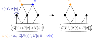
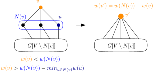
Figure 1: Neighbor removal (left) and neighborhood folding (right)

5.1 Meta Reductions.

There are two operations that are commonly used in reductions: vertex removal and vertex folding. In the following reductions, we show general ways to detect when these operations can be applied in the neighborhood of a vertex.

Neighbor Removal. In our first meta reduction, we show how to determine if a neighbor can be outright removed from the graph. We call this reduction the neighbor removal reduction. (See Figure 1.)

Reduction 2 (Neighbor Removal)

Let $v\in V$. For any $u\in N(v)$, if $\alpha_{w}(G[N(v)\setminus N[u]])+w(u)\leq w(v)$, then $u$ can be removed from $G$, as there is some MWIS of $G$ that excludes $u$, and $\alpha_{w}(G)=\alpha_{w}(G[V\setminus\{u\}])$.

• Let ${\mathcal{I}}$ be an MWIS of $G$. We show by a cut-and-paste argument that if $u\in{\mathcal{I}}$ then there is another MWIS ${\mathcal{I}}^{\prime}$ that contains $v$ instead. Let $u\in N(v)$, and suppose that $\alpha_{w}(G[N(v)\setminus N[u]])+w(u)\leq w(v)$. There are two cases, if $u$ is not in ${\mathcal{I}}$ then it is safe to remove. Otherwise, suppose $u\in{\mathcal{I}}$. Then $v\in N(u)$ is not in ${\mathcal{I}}$, and $w({\mathcal{I}}\cap N(v))=w({\mathcal{I}}\cap(N(v)\setminus N[u])\cup\{u\})=\alpha_{w}(G[N(v)\setminus N[u]])+w(u)=w(v)$; otherwise we can swap ${\mathcal{I}}\cap N(v)$ for $v$ in ${\mathcal{I}}$ obtaining an independent set of larger weight. Thus ${\mathcal{I}}^{\prime}=({\mathcal{I}}\setminus N(v))\cup\{v\}$ is an MWIS of $G$ excluding $u$ and $\alpha_{w}(G)=\alpha_{w}(G[V\setminus\{u\}])$.   $\boxtimes$

Neighborhood Folding. For our next meta reduction, we show a general condition for folding a vertex with its neighborhood. We first briefly describe the intuition behind the reduction. Consider $v$ and its neighborhood $N(v)$. If $N(v)$ has a unique independent set ${\mathcal{I}}_{N(v)}$ with weight larger than $w(v)$, then we only need to consider two independent sets: independent sets that contain $v$ or ${\mathcal{I}}_{N(v)}$. Otherwise, any other independent set in $N(v)$ can be swapped for $v$ and achieve higher overall weight. By folding $v$ with ${\mathcal{I}}_{N(v)}$, we can solve the remaining graph and then decide which of the two options will give an MWIS of the graph. (See Figure 1.)

Reduction 3 (Neighborhood Folding)

Let $v\in V$, and suppose that $N(v)$ is independent. If $w(N(v))>w(v)$, but $w(N(v))-\min_{u\in N(v)}\{w(u)\}<w(v)$, then fold $v$ and $N(v)$ into a new vertex $v^{\prime}$ with weight $w(v^{\prime})=w(N(v))-w(v)$. Let ${\mathcal{I}}^{\prime}$ be an MWIS of $G^{\prime}$, then we construct an MWIS ${\mathcal{I}}$ of $G$ as follows: If $v^{\prime}\in{\mathcal{I}}^{\prime}$ then ${\mathcal{I}}=({\mathcal{I}}^{\prime}\setminus\{v^{\prime}\})\cup N(v)$, otherwise if $v\in{\mathcal{I}}^{\prime}$ then ${\mathcal{I}}={\mathcal{I}}^{\prime}\cup\{v\}$. Furthermore, $\alpha_{w}(G)=\alpha_{w}(G^{\prime})+w(v)$.

• Proof can be found in Appendix A.   $\boxtimes$

However, these reductions require solving the MWIS problem on the neighborhood of a vertex, and therefore may be as expensive as computing an MWIS on the input graph. We next show how to use these meta reductions to develop efficient reductions.

5.2 Efficient Weighted Reductions.

We now construct new efficient reductions using the just defined meta reductions.

Neighborhood Removal. In their HILS local search algorithm, Nogueria et al. [27] introduced the notion of a “$(\omega,1)$-swap”, which swaps a vertex $v$ into a solution if its neighbors in the current solution $I$ have weight $w(N(v)\cap I)<w(v)$. This can be transformed into what we call the neighborhood removal reduction.

Reduction 4 (Neighorhood Removal)

For any $v\in V$, if $w(v)\geq w(N(v))$ then $v$ is in some MWIS of $G$. Let $G^{\prime}=G[V\setminus N[v]]$ and $\alpha_{w}(G)=\alpha_{w}(G^{\prime})+w(v)$.

Since $w(N(v))\leq w(v)$, $\forall u\in N(v)$ we have that

$$\alpha_{w}(G[N(v)\cap N(u)])+w(u)\leq w(N(v))\leq w(v).$$

Then we can remove all $u\in N(v)$ and are left with $v$ in its own component. Calling this graph $G^{\prime}$, we have that $v$ is in some MWIS and $\alpha_{w}(G)=\alpha_{w}(G^{\prime})+w(v)$.   $\boxtimes$

For the remaining reductions, we assume that the neighborhood removal reduction has already been applied. Thus, $\forall v\in V$, $w(v)<w(N(v))$.

Weighted Isolated Vertex Removal. Similar to the (unweighted) isolated vertex removal reduction, we now argue that an isolated vertex is in some MWIS—if it has highest weight in its clique.

Reduction 5 (Isolated Vertex Removal.)

Let $v\in V$ be isolated and $w(v)\geq\max_{u\in N(v)}w(u)$. Then $v$ is in some MWIS of $G$. Let $G^{\prime}=G[V\setminus N[v]]$ and $\alpha_{w}(G)=\alpha_{w}(G^{\prime})+w(v)$.

• Since $N(v)$ is a clique, $\forall u\in N(v)$ we have that

  $$\alpha_{w}(G[N(v)\cap N(u)])\leq\alpha_{w}(N(v))=\max_{u\in N(v)}\{w(u)\}\leq w(v).$$

  Similar to neighborhood removal, remove all $u\in N(v)$ producing $G^{\prime}$ and $\alpha_{w}(G)=\alpha_{w}(G^{\prime})+w(v)$.   $\boxtimes$

Isolated Weight Transfer. Given its weight restriction, the weighted isolated vertex removal reduction may be ineffective. We therefore introduce a reduction that supports more liberal vertex removal.

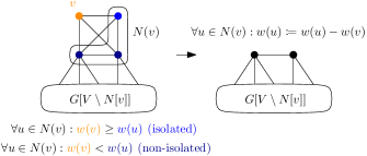
Figure 2: Isolated weight transfer

Reduction 6 (Isolated weight transfer)

Let $v\in V$ be isolated, and suppose that the set of isolated vertices $S(v)\subseteq N(v)$ is such that $\forall u\in S(v)$, $w(v)\geq w(u)$. We

1. remove all $u\in N(v)$ such that $w(u)\leq w(v)$, and let the remaining neighbors be denoted by $N^{\prime}(v)$,

2. remove $v$ and $\forall x\in N^{\prime}(v)$ set its new weight to $w^{\prime}(x)=w(x)-w(v)$, and

let the resulting graph be denoted by $G^{\prime}$. Then $\alpha_{w}(G)=w(v)+\alpha_{w}(G^{\prime})$ and an MWIS ${\mathcal{I}}$ of $G$ can be constructed from an MWIS ${\mathcal{I}}^{\prime}$ of $G^{\prime}$ as follows: if ${\mathcal{I}}^{\prime}\cap N^{\prime}(v)=\emptyset$ then ${\mathcal{I}}={\mathcal{I}}^{\prime}\cup\{v\}$, otherwise ${\mathcal{I}}={\mathcal{I}}^{\prime}$.

• Proof can be found in Appendix A.  $\boxtimes$

Weighted Vertex Folding. Similar to the unweighted vertex folding reduction, we show that we can fold vertices with two non-adjacent neighbors—however, not all weight configurations permit this.

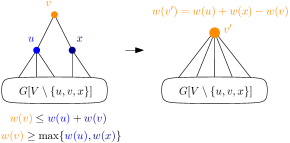
Figure 3: Weighted vertex folding

Reduction 7 (Vertex Folding)

Let $v\in V$ have $d(v)=2$, such that $v$’s neighbors $u$, $x$ are not adjacent. If $w(v)<w(u)+w(x)$ but $w(v)\geq\max\{w(u),w(x)\}$, then we fold $v,u,x$ into vertex $v^{\prime}$ with weight $w(v^{\prime})=w(u)+w(x)-w(v)$ forming a new graph $G^{\prime}$. Then $\alpha_{w}(G)=\alpha_{w}(G^{\prime})+w(v)$. Let $\mathcal{I}^{\prime}$ be an MWIS of $G^{\prime}$. If $v^{\prime}\in\mathcal{I}^{\prime}$ then ${\mathcal{I}}=({\mathcal{I}}^{\prime}\setminus\{v^{\prime}\})\cup\{u,x\}$ is an MWIS of $G$. Otherwise, ${\mathcal{I}}={\mathcal{I}}^{\prime}\cup\{v\}$ is an MWIS of $G$.

• Apply neighborhood folding to $v$.   $\boxtimes$

Weighted Twin.

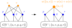
Figure 4: Illustrating proof of weighted twin reduction

The twin reduction, as described by Akiba and Iwata [3] for the unweighted case, works for twins with $3$ common neighbors. We describe our variant in the same terms, but note that the reduction supports an arbitrary number of common neighbors.

Reduction 8 (Twin)

Let vertices $u$ and $v$ have independent neighborhoods $N(u)=N(v)=\{p,q,r\}$. We have two cases:

1. If $w(\{u,v\})\geq w(\{p,q,r\})$, then $u$ and $v$ are in some MWIS of $G$. Let $G^{\prime}=G[V\setminus N[\{u,v\}]]$.

2. If $w(\{u,v\})<w(\{p,q,r\})$, but $w(\{u,v\})>w(\{p,q,r\})-\min_{x\in\{p,q,r\}}w(x)$, then we can fold $u,v,p,q,r$ into a new vertex $v^{\prime}$ with weight $w(v^{\prime})=w(\{p,q,r\})-w(\{u,v\})$ and call this graph $G^{\prime}$. Let $I^{\prime}$ be an MWIS of $G^{\prime}$. Then we construct an MWIS ${\mathcal{I}}$ of $G$ as follows: if $v^{\prime}\in{\mathcal{I}}^{\prime}$ then ${\mathcal{I}}=({\mathcal{I}}^{\prime}\setminus\{v^{\prime}\})\cup\{p,q,r\}$, if $v^{\prime}\notin{\mathcal{I}}^{\prime}$ then ${\mathcal{I}}={\mathcal{I}}^{\prime}\cup\{u,v\}$.

Furthermore, $\alpha_{w}(G)=\alpha_{w}(G^{\prime})+w(\{u,v\})$.

• Just as in the unweighted case, either $u$ and $v$ are simultaneously in an MWIS or some subset of $p$, $q$, $r$ is in. First fold $u$ and $v$ into a new vertex $\{u,v\}$ with weight $w(\{u,v\})$. To show (i), apply the neighborhood reduction to vertex $\{u,v\}$. For (ii), since $N(\{u,v\})$ is independent, we apply the neighborhood folding reduction to $\{u,v\}$, giving the claimed result.  $\boxtimes$

If $p,q,r$ are not independent, further reductions are possible; however, introducing a comprehensive list is not illuminating. Instead, we can simply let meta reductions reduce as appropriate.

Weighted Domination. Lastly, we give a weighted variant of the domination reduction.

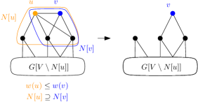
Figure 5: Weighted domination

Reduction 9 (Domination)

Let $u,v\in V$ be vertices such that $N[u]\supseteq N[v]$ (i.e., $u$ dominates $v$). If $w(u)\leq w(v)$, there is an MWIS in $G$ that excludes $u$ and $\alpha_{w}(G)=\alpha_{w}(G[V\setminus\{u\}])$. Therefore, $u$ can be removed from the graph.

• We show by a cut-and-paste argument that there is an MWIS of $G$ excluding $u$. Let ${\mathcal{I}}$ be an MWIS of $G$. If $u$ is not in ${\mathcal{I}}$ then we are done. Otherwise, suppose $u\in{\mathcal{I}}$. Then it must be the case that $w(v)=w(u)$, otherwise ${\mathcal{I}}^{\prime}=({\mathcal{I}}\setminus\{u\})\cup\{v\}$ is an independent set with weight larger than ${\mathcal{I}}$. Thus, ${\mathcal{I}}^{\prime}$ is an MWIS of $G$ excluding $u$, and $\alpha_{w}(G)=\alpha_{w}(G[V\setminus\{u\}])$.   $\boxtimes$

6 Experimental Evaluation

We now compare the performance of our branch-and-reduce algorithm to existing state-of-the-art algorithms on large real-world graphs. Furthermore, we examine how our reduction rules can drastically improve the quality of existing heuristic approaches.

6.1 Methodology and Setup.

All of our experiments were run on a machine with four Octa-Core Intel Xeon E5-4640 processors running at $2.4$ GHz, $512$ GB of main memory, $420$ MB L3-Cache and $48256$ KB L2-Cache. The machine runs Ubuntu 14.04.3 and Linux kernel version 3.13.0-77. All algorithms were implemented in C++-11 and compiled with g++ version 4.8.4 with optimization flag -O3. Each algorithm was run sequentially for a total of $1000$ seconds. We present two kinds of data: (1) the best solution found by each algorithm and the time (in seconds) required to obtain it, (2) convergence plots, which show how the solution quality changes over time. In particular, whenever an algorithm finds a new best independent set $S$ at time $t$, it reports a tuple ($t$, $|S|$).

Graph	$|V|$	$t_{\text{max}}$	$w_{\text{max}}$	$t_{\text{max}}$	$w_{\text{max}}$	$t_{\text{max}}$	$w_{\text{max}}$
OSM networks		DynWVC1		HILS		B & Rdense
alabama-AM3	3 504	464.02	185 527	0.73	185 744	15.79	185 707
florida-AM2	1 254	1.14	230 595	0.04	230 595	0.03	230 595
georgia-AM3	1 680	0.88	222 652	0.05	222 652	4.88	214 918
kansas-AM3	2 732	46.87	87 976	0.84	87 976	11.35	87 925
maryland-AM3	1 018	1.34	45 496	0.02	45 496	3.34	45 496
massachusetts-AM3	3 703	435.31	145 863	2.73	145 866	12.87	145 617
utah-AM3	1 339	136.15	98 802	0.08	98 847	64.04	98 847
vermont-AM3	3 436	119.63	63 234	0.95	63 302	95.81	55 584
Solved instances						44.12% (15/34)
Optimal weight		60.00% (9/15)		100.00% (15/15)
SNAP networks		DynWVC2		HILS		B & Rfull
as-skitter	1 696 415	576.93	123 105 765	998.75	122 539 706	746.93	123 904 741
ca-AstroPh	18 772	108.35	796 535	46.76	796 556	0.03	796 556
email-EuAll	265 214	179.26	25 330 331	501.09	25 330 331	0.19	25 330 331
p2p-Gnutella08	6 301	0.19	435 893	0.25	435 893	0.01	435 893
roadNet-TX	1 379 917	1 000.78	77 525 099	1 697.13	76 366 577	33.49	78 606 965
soc-LiveJournal1	4 847 571	1 001.23	277 824 322	12 437.50	280 559 036	270.96	283 948 671
web-Google	875 713	683.63	56 190 870	994.58	55 954 155	3.16	56 313 384
wiki-Talk	2 394 385	991.31	235 874 419	996.02	235 852 509	3.36	235 875 181
Solved instances						80.65% (25/31)
Optimal weight		28.00% (7/25)		68.00% (17/25)

Table 1: Best solution found by each algorithm and time (in seconds) required to compute it. The global best solution is highlighted in bold. Rows are highlighted in gray if B & R is able to find an exact solution.

Algorithms Compared. We use two different variants of our branch-and-reduce algorithm. The first variant, called B & R_full, uses our full set of reductions each time we branch. The second variant, called B & R_dense, omits the more costly reductions and also terminates the execution of the remaining reductions faster than B & R_full. In particular, this configuration completely omits the weighted critical set reductions from both the initialization and recursion. Additionally, we also omit the weighted clique reduction from the first reduction call and use a faster version that only considers triangles during recursion. Finally, we do not use the generalized neighborhood folding during recursion. This configuration find solutions more quickly on dense graphs.

We also include the state-of-the-art heuristics HILS by Nogueria et al. [27] and both versions of DynWVC by Cai et al. [13] (see Section 2 for a short explanation of these algorithms). Finally, we do not include any other exact algorithms (e.g.  [10, 32]) as their code is not available. Also note that these exact algorithms are either not tested in the weighted case [10] or the largest instances reported consist of a few hundred vertices [32].

To further evaluate the impact of reductions on existing algorithms, we also propose combinations of the heuristic approaches with reductions (Red + HILS and Red + DynWVC). We do so by first computing a kernel graph using our set of reductions and then run the existing algorithms on the resulting graph.

Instances. We test all algorithms on a large corpus of sparse data sets. For this purpose, we include a set of real-world conflict graphs obtained from OpenStreetMap [1] files of North America, according to the method described by Barth et al. [7]. More specifically, these graphs are generated by identifying map labels with vertices that have a weight corresponding to their importance. Edges are then inserted between vertices if their labels overlap each other. Conflict graphs can also be used in a dynamic setting by associating vertices with intervals that correspond to the time they are displayed. Furthermore, solving the MWIS problem on these graphs eliminates label conflicts and maximizes the importance of displayed labels. Finally, different activity models (AM1, AM2 and AM3) are used to generate different conflict graphs. The instances we use for our experiments are the same ones used by Cai et al. [13]. We omit all instances with less than $1000$ vertices from our experiments, as these are easy to solve and our focus is on large scale networks [13].

In addition to the OSM networks, we also include collaboration networks, communication networks, additional road networks, social networks, peer-to-peer networks, and Web crawl graphs from the Stanford Large Network Dataset Repository [24] (SNAP).

These networks are popular benchmark instances commonly used for the maximum independent set problem [3, 16, 22]. However, all SNAP instances are unweighted and comparable weighted instances are very scarce. Therefore, a common approach in literature is to assign vertex weights uniformly at random from a fixed size interval [13, 25]. To keep our results in line with existing work, we thus decided to select vertex weights uniformly at random from $[1,200]$. Basic properties of our benchmark instances can be found in Table 3.

6.2 Comparison with State-of-the-Art.

A representative sample of our experimental results for the OSM and SNAP networks is presented in Table 1. For a full overview of all instances, we refer to Table 4 (OSM) and Table 5 (SNAP) respectively. For each instance, we list the best solution computed by each algorithm $w_{\text{Algo}}$ and the time in seconds required to find it $t_{\text{Algo}}$. For each data set, we highlight the best solution found across all algorithms in bold. Additionally, if any version of our algorithm is able to find an exact solution, the corresponding row is highlighted in gray. Finally, recall that our algorithm computes a solution on unsolved instances once the time-limit is reached by additionally running a greedy algorithm as post-processing.

Examining the OSM graphs, B & R is able to solve 15 out of the 34 instances we tested. However, HILS is also able to compute a solution with the same weight on all of these instance. Furthermore, HILS obtains a higher or similar quality solution than both versions of DynWVC and B & R for all remaining unsolved instances. Overall, HILS is able to find the best solution on all OSM instances that we tested. Additionally, on most of these instances it does so significantly faster than all of its competitors. Note though, that neither HILS nor DynWVC provide any optimality guarantees (in contrast to B & R).

Looking at both versions of DynWVC, we see that DynWVC1 performs better than DynWVC2, which is also reported by Cai et al. [13]. Comparing both variants of our branch-and-reduce algorithm, we see that they are able to solve the same instances. Nonetheless, B & R_dense is able to compute better solutions on roughly half of the remaining instances. Additionally, it almost always requires significantly less time to achieve its maximum compared to B & R_full.

Figure 6: Solution quality over time for two OSM instances (left) and two SNAP instances (right).

Graph	$t_{\text{max}}$	$w_{\text{max}}$	$t_{\text{max}}$	$w_{\text{max}}$	$S_{\text{base}}$	$t_{\text{max}}$	$w_{\text{max}}$	$t_{\text{max}}$	$w_{\text{max}}$	$S_{\text{base}}$	$t_{\text{max}}$	$w_{\text{max}}$
OSM instances	DynWVC1		Red+DynWVC1			HILS		Red + HILS			B & Rdense
alabama-AM3	464.02	185 527	370.80	185 727	1.25	0.73	185 744	4.05	185 744	0.18	15.79	185 707
florida-AM2	1.14	230 595	0.03	230 595	44.19	0.04	230 595	0.03	230 595	1.75	0.03	230 595
georgia-AM3	0.88	222 652	2.64	222 652	0.33	0.05	222 652	2.43	222 652	0.02	4.88	214 918
kansas-AM3	46.87	87 976	13.59	87 976	3.45	0.84	87 976	2.06	87 976	0.41	11.35	87 925
maryland-AM3	1.34	45 496	2.07	45 496	0.65	0.02	45 496	2.07	45 496	0.01	3.34	45 496
massachusetts-AM3	435.31	145 863	10.68	145 866	40.75	2.73	145 866	2.92	145 866	0.93	12.87	145 617
utah-AM3	136.15	98 802	168.07	98 847	0.81	0.08	98 847	2.10	98 847	0.04	64.04	98 847
vermont-AM3	119.63	63 234	62.85	63 280	1.90	0.95	63 302	2.95	63 312	0.32	95.81	55 584
Solved instances											44.12% (15/34)
Optimal weight	60.00% (9/15)		93.33% (14/15)			100.00% (15/15)		100.00% (15/15)
SNAP instances	DynWVC2		Red+DynWVC2			HILS		Red + HILS			B & Rdense
as-skitter	576.93	123 105 765	85.60	123 995 808	6.74	998.75	122 539 706	845.70	123 996 322	1.18	746.93	123 904 741
ca-AstroPh	108.35	796 535	0.02	796 556	4 962.17	46.76	796 556	0.02	796 556	2 142.48	0.03	796 556
email-EuAll	179.26	25 330 331	0.12	25 330 331	1 548.08	501.09	25 330 331	0.12	25 330 331	4 327.82	0.19	25 330 331
p2p-Gnutella08	0.19	435 893	0.00	435 893	46.98	0.25	435 893	0.00	435 893	63.80	0.01	435 893
roadNet-TX	1 000.78	77 525 099	771.05	78 601 813	1.30	1 697.13	76 366 577	946.32	78 602 984	1.79	33.49	78 606 965
soc-LiveJournal1	1 001.23	277 824 322	996.68	283 973 997	1.00	12 437.50	280 559 036	761.51	283 975 036	16.33	270.96	283 948 671
web-Google	683.63	56 190 870	3.30	56 313 349	207.26	994.58	55 954 155	3.01	56 313 384	330.28	3.16	56 313 384
wiki-Talk	991.31	235 874 419	2.30	235 875 181	430.22	996.02	235 852 509	2.30	235 875 181	432.26	3.36	235 875 181
Solved instances											80.65% (25/31)
Optimal weight	28.00% (7/25)		84.00% (21/25)			68.00% (17/25)		88.00% (22/25)

Table 2: Best solution found by each algorithm and time (in seconds) required to compute it. $S_{\text{base}}=\frac{t_{\text{base}}}{t_{\text{modified}}}$ denotes the speedup between the modified and base versions of each local search. The global best solution is highlighted in bold. Rows are highlighted in gray if B & R is able to find an exact solution.

For the SNAP networks, we see that B & R solves $25$ of the $31$ instances we tested . Most notable, on seven of these instances where either HILS or DynWVC1 also find a solution with optimal weight, it does so up to two orders of magnitude faster. This difference in performance compared to the OSM networks can be explained by the significantly lower graph density and less uniform degree distribution of the SNAP networks. These structural differences seem to allow for our reduction rules to be applicable more often, resulting in a significantly smaller kernel (as seen in Table 3). This is similar to the behavior of unweighted branch-and-reduce [3]. Therefore, except for a single instance, our algorithm is able to find the best solution on all graphs tested.

Comparing the heuristic approaches, both versions of DynWVC perform better than HILS on most instances, with DynWVC2 often finding better solution than DynWVC1. Nonetheless, HILS finds higher weight solutions than DynWVC1 and DynWVC2.

6.3 The Power of Weighted Reductions.

We now examine the effect of using reductions to improve existing heuristic algorithms. For this purpose, we compare the combined approaches Red + HILS and Red + DynWVC with their base versions as well as our branch-and-reduce algorithm. Our sample of results for the OSM and SNAP networks is given in Table 2. In addition to the data used in our state-of-the-art comparison, we now also report speedups between the modified and base versions of each local search. Additionally, we give the percentage of instances solved by B & R, as well as the percentage of solutions with optimal weight found be the inexact algorithms compared to B & R. For a full overview of all instances, we refer to Table 6 and Table 7 respectively.

When looking at the speedups for the SNAP graphs, we can see that using reductions allows local search to find optimal solutions orders of magnitude faster. Additionally, they are now able to find an optimal solution more often than without reductions. DynWVC2 in particular achieves an increase of $56\%$ of optimal solutions when using reductions. Overall, we achieve a speedup of up to three orders of magnitude for the SNAP instances. Thus, the additional costs for computing the kernel can be neglected for these instances. However, for the OSM instances our reduction rules are less applicable and reducing the kernel comes at a significant cost compared to the unmodified local searches.

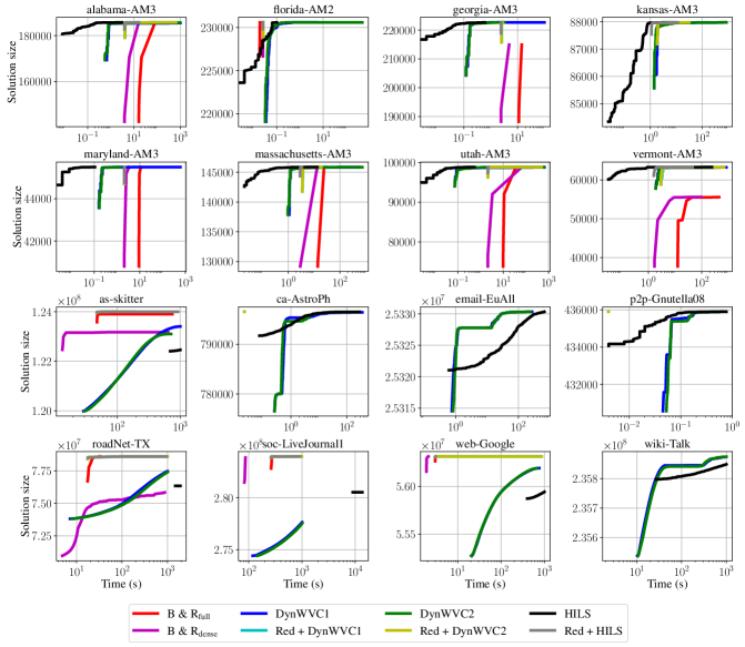
Figure 7: Solution quality over time for our sample of eight OSM instances (upper two rows) and eight SNAP instances (lower two rows) as given in Section 6.2.

To further examine the influence of using reductions, Figure 6 shows the solution quality over time for all algorithms and four instances. For additional convergence plots, we refer to Figure 7. For the OSM instances, we can see that initially DynWVC and HILS are able find good quality solutions much faster compared to their combined approaches. However, once the kernel has been computed, regular DynWVC and HILS are quickly outperformed by the hybrid algorithms.

A more drastic change can be seen for the SNAP instances. Instances were both DynWVC and HILS examine poor performance, Red + DynWVC and Red + HILS now rival our branch-and-reduce algorithm and give near-optimal solutions in less time. Thus, using reductions for instances that are too large for traditional heuristic approaches allows for a drastic improvement.

7 Conclusion and Future Work

In this paper, we engineered a new branch-and-reduce algorithm as well as a combination of kernelization with local search for the maximum weight independent set problem. The core of our algorithms are a full suite of new reductions for the maximum weight independent set problem. We performed extensive experiments to show the effectiveness of our algorithms in practice on real-world graphs of up to millions of vertices and edges. Our experimental evaluation shows that our branch-and-reduce algorithm can solve many large real-world instances quickly in practice, and that kernelization has a highly positive effect on local search algorithms.

As HILS often finds optimal solutions in practice, important future works include using this algorithm for the lower bound computation within our branch-and-reduce algorithm. Furthermore, we would like to extend our discussion on the effectiveness of novel reduction rules. In particular, we want to evaluate how much quality we gain from applying each individual rule and how the order we apply them in changes the resulting kernel size.

A Omitted Proofs

Reduction 3 (Neighborhood Folding)

Let $v\in V$, and suppose that $N(v)$ is independent. If $w(N(v))>w(v)$, but $w(N(v))-\min_{u\in N(v)}\{w(u)\}<w(v)$, then fold $v$ and $N(v)$ into a new vertex $v^{\prime}$ with weight $w(v^{\prime})=w(N(v))-w(v)$. Let ${\mathcal{I}}^{\prime}$ be an MWIS of $G^{\prime}$, then we construct an MWIS ${\mathcal{I}}$ of $G$ as follows: If $v^{\prime}\in{\mathcal{I}}^{\prime}$ then ${\mathcal{I}}=({\mathcal{I}}^{\prime}\setminus\{v^{\prime}\})\cup N(v)$, otherwise if $v\in{\mathcal{I}}^{\prime}$ then ${\mathcal{I}}={\mathcal{I}}^{\prime}\cup\{v\}$. Furthermore, $\alpha_{w}(G)=\alpha_{w}(G^{\prime})+w(v)$.

• First note that after folding, the following graphs are identical: $G^{\prime}[V^{\prime}\setminus N_{G^{\prime}}[v^{\prime}]]=G[V\setminus N[N[v]]$ and $G^{\prime}[V^{\prime}\setminus\{v^{\prime}\}]=G[V\setminus N[v]]$. Let ${\mathcal{I}}^{\prime}$ be an MWIS of $G^{\prime}$. We have two cases.

  Case 1 ($v^{\prime}\in{\mathcal{I}}^{\prime}$): Suppose that $v^{\prime}\in{\mathcal{I}}^{\prime}$. We show that $w(N(v))+\alpha_{w}(G[V\setminus N[N[v]]])\geq w(v)+\alpha_{w}(G[V\setminus N[v]])$, which shows that the vertices of $N(v)$ are together in some MWIS of $G$. Since $v^{\prime}\in{\mathcal{I}}^{\prime}$, we have that

  $$w(v)+\alpha_{w}(G^{\prime}) =w(v)+w(v^{\prime})+\alpha_{w}(G^{\prime}[V^{\prime}\setminus N_{G^{\prime}}[v^{\prime}]])$$

  $$=w(v)+w(N(v))-w(v)$$

  $$\phantom{=w(v)+w(N(v))\text{ }}+\alpha_{w}(G^{\prime}[V^{\prime}\setminus N_{G^{\prime}}[v^{\prime}]])$$

  $$=w(N(v))+\alpha_{w}(G[V\setminus N[N[v]]]).$$

  But since ${\mathcal{I}}^{\prime}$ is an MWIS of $G^{\prime}$, we have that

  $$w(v)+\alpha_{w}(G^{\prime}) \geq w(v)+\alpha_{w}(G^{\prime}[V^{\prime}\setminus\{v^{\prime}\}])$$

  $$=w(v)+\alpha_{w}(G[V\setminus N[v]]).$$

  Thus, $w(N(v))+\alpha_{w}(G[V\setminus N[N[v]]])\geq w(v)+\alpha_{w}(G[V\setminus N[v]])$ and the vertices of $N(v)$ are together in some MWIS of $G$. Furthermore, we have that

  $$\alpha_{w}(G) =w(N(v))+\alpha_{w}(G[V\setminus N[N[v]]])$$

  $$=\alpha_{w}(G^{\prime})+w(v).$$

  Case 2: ($v^{\prime}\notin{\mathcal{I}}^{\prime}$): Suppose that $v^{\prime}\notin{\mathcal{I}}^{\prime}$. We show that $w(v)+\alpha_{w}(G[V\setminus N[v]])\geq w(N(v))+\alpha_{w}(G[V\setminus N[N[v]]])$, which shows that $v$ is in some MWIS of $G$. Since $v^{\prime}\notin{\mathcal{I}}^{\prime}$, we have that

  $$w(v)+\alpha_{w}(G^{\prime}) =w(v)+\alpha_{w}(G^{\prime}[V^{\prime}\setminus\{v^{\prime}\}])$$

  $$=w(v)+\alpha_{w}(G[V\setminus N[v]])$$

  But since ${\mathcal{I}}^{\prime}$ is an MWIS of $G^{\prime}$, we have that

  $$w(v)+\alpha_{w}(G^{\prime}) \geq w(v)+w(v^{\prime})+\alpha_{w}(G^{\prime}[V^{\prime}\setminus N_{G^{\prime}}[v^{\prime}]])$$

  $$=w(v)+w(N(v))-w(v)$$

  $$\phantom{=w(v)+w(N(v))\text{ }}+\alpha_{w}(G[V\setminus N[N[v]]])$$

  $$=w(N(v))+\alpha_{w}(G[V\setminus N[N[v]]]).$$

  Thus, $w(v)+\alpha_{w}(G[V\setminus N[v]])\geq w(u)+w(x)+\alpha_{w}(G[V\setminus N[\{u,x\}]])$ and $v$ is in some MWIS of $G$. Lastly,

  $$\alpha_{w}(G) =w(v)+\alpha_{w}(G[V\setminus N[v]])$$

  $$=\alpha_{w}(G^{\prime})+w(v).$$

  $\boxtimes$

Reduction 6 (Isolated weight transfer)

Let $v\in V$ be isolated, and suppose that the set of isolated vertices $S(v)\subseteq N(v)$ is such that $\forall u\in S(v)$, $w(v)\geq w(u)$. We

1. remove all $u\in N(v)$ such that $w(u)\leq w(v)$, and let the remaining neighbors be denoted by $N^{\prime}(v)$,

2. remove $v$ and $\forall x\in N^{\prime}(v)$ set its new weight to $w^{\prime}(x)=w(x)-w(v)$, and

let the resulting graph be denoted by $G^{\prime}$. Then $\alpha_{w}(G)=w(v)+\alpha_{w}(G^{\prime})$ and an MWIS ${\mathcal{I}}$ of $G$ can be constructed from an MWIS ${\mathcal{I}}^{\prime}$ of $G^{\prime}$ as follows: if ${\mathcal{I}}^{\prime}\cap N^{\prime}(v)=\emptyset$ then ${\mathcal{I}}={\mathcal{I}}^{\prime}\cup\{v\}$, otherwise ${\mathcal{I}}={\mathcal{I}}^{\prime}$.

• For (i), note that it is safe to remove all $u\in N(v)$ such that $w(u)\leq w(v)$ since these vertices meet the criteria for the neighbor removal reduction. All vertices $x\in N^{\prime}(v)$ that remain have weight $w(x)>w(v)$ and are not isolated.

  Case 1 (${\mathcal{I}}^{\prime}\cap N^{\prime}(v)=\emptyset$): Let ${\mathcal{I}}^{\prime}$ be an MWIS of $G^{\prime}$, we show that if ${\mathcal{I}}^{\prime}\cap N^{\prime}(v)=\emptyset$ then $I=I^{\prime}\cup\{v\}$. To show this, we show that $w(v)+\alpha_{w}(G[V\setminus N[v]])\geq\alpha_{w}(G[V\setminus\{v\}])$.

  Let $x\in N^{\prime}(v)$. Since $x\notin I^{\prime}$, we have that

  $$w(v)+\alpha_{w}(G^{\prime}) =w(v)+\alpha_{w}(G^{\prime}[V^{\prime}\setminus N^{\prime}(v)])$$

  $$=w(v)+\alpha_{w}(G[V\setminus N[v]])$$

  and

  $$w(v)+\alpha_{w}(G^{\prime}) \geq w(v)+w^{\prime}(x)+\alpha_{w}(G^{\prime}[V^{\prime}\setminus N[x]])$$

  $$=w(v)+w(x)-w(v)+\alpha_{w}(G^{\prime}[V^{\prime}\setminus N[x]])$$

  $$=w(x)+\alpha_{w}(G[V\setminus N[x]]).$$

  Thus, for any $x\in N^{\prime}(v)$, we have that

  $$w(v)+\alpha_{w}(G^{\prime}) =w(v)+\alpha_{w}(G[V\setminus N[v]])$$

  $$\geq w(x)+\alpha_{w}(G[V\setminus N[x]])$$

  and therefore the heaviest independent set containing $v$ is at least the weight of the heaviest independent containing any neighbor of $v$. Concluding, we have that

  $$w(v)+\alpha_{w}(G[V\setminus N[v]])\geq\alpha_{w}(G[V\setminus\{v\}])$$

  and therefore ${\mathcal{I}}={\mathcal{I}}^{\prime}\cup\{v\}$ is an MWIS of $G$.

  Case 2 (${\mathcal{I}}^{\prime}\cap N^{\prime}(v)\neq\emptyset$): Let ${\mathcal{I}}^{\prime}$ be an MWIS of $G^{\prime}$, we show that if ${\mathcal{I}}^{\prime}\cap N^{\prime}(v)\neq\emptyset$ then ${\mathcal{I}}={\mathcal{I}}^{\prime}$. To show this, let $\{x\}={\mathcal{I}}^{\prime}\cap N^{\prime}(v)$. Define $G^{\prime\prime}$ as the graph resulting from increasing the weight of $N^{\prime}(v)$ by $w(v)$, i.e.  $\forall~{}u~{}\in~{}N^{\prime}(v)$ we set $w^{\prime\prime}(u)=w^{\prime}(u)+w(v)=w(u)$. We first show that ${\mathcal{I}}^{\prime\prime}={\mathcal{I}}^{\prime}$ is an MWIS of $G^{\prime}$. Therefore, assume that ${\mathcal{I}}^{*}$ is an MWIS of $G^{\prime\prime}$ with $w({\mathcal{I}}^{*})>w({\mathcal{I}}^{\prime})$ that does not contain $x$. However, then ${\mathcal{I}}^{*}$ is also a better MWIS on $G^{\prime}$ which contradicts our initial assumption. Finally, we have that $w({\mathcal{I}}^{\prime\prime})=w({\mathcal{I}}^{\prime})+w(v)$, since exactly one node in $N^{\prime}(v)$ is in ${\mathcal{I}}^{\prime}$.

  Next, we define $G^{\prime\prime\prime}$ as the graph resulting from adding back $v$ to $G^{\prime}$’ and show that ${\mathcal{I}}^{\prime\prime\prime}={\mathcal{I}}^{\prime\prime}$ is a MWIS of $G^{\prime\prime\prime}$. For this purpose, we assume that ${\mathcal{I}}^{*}$ is a MWIS of $G^{\prime\prime\prime}$ with $w({\mathcal{I}}^{*})>w({\mathcal{I}}^{\prime\prime\prime})$. Then, $v\in{\mathcal{I}}^{*}$ since we only added this node to $G^{\prime\prime}$. Likewise, $x\not\in{\mathcal{I}}^{*}$ since its a neighbor of $v$.

  Since $w({\mathcal{I}}^{*})>w({\mathcal{I}}^{\prime\prime\prime})$, we have that:

  $$w({\mathcal{I}}^{*}\setminus\{v\}) =w({\mathcal{I}}^{*})-w(v)$$

  $$>w({\mathcal{I}}^{\prime\prime})-w(v)$$

  $$=w({\mathcal{I}}^{\prime})+w(v)-w(v)$$

  $$=w({\mathcal{I}}^{\prime}).$$

  However, since ${\mathcal{I}}^{*}\setminus\{v\}$ does neither include v nor any neighbor of $v$ it is also an IS of $G^{\prime}$ that is larger than ${\mathcal{I}}^{\prime}$. This contradicts our initial assumption and thus ${\mathcal{I}}^{\prime\prime\prime}={\mathcal{I}}^{\prime\prime}={\mathcal{I}}^{\prime}$. Furthermore, since $G^{\prime\prime\prime}=G$, we have that ${\mathcal{I}}^{\prime\prime\prime}={\mathcal{I}}={\mathcal{I}}^{\prime}$.   $\boxtimes$

B Graph Properties, Kernel Sizes, Full Tables, Convergence Plots

Graph	$|V|$	$|E|$	$\mathcal{K}_{\text{dense}}$	$\mathcal{K}_{\text{full}}$
alabama-AM2	1 164	38 772	173	173
alabama-AM3	3 504	619 328	1 614	1 614
district-of-columbia-AM1	2 500	49 302	800	800
district-of-columbia-AM2	13 597	3 219 590	6 360	6 360
district-of-columbia-AM3	46 221	55 458 274	33 367	33 367
florida-AM2	1 254	33 872	41	41
florida-AM3	2 985	308 086	1 069	1 069
georgia-AM3	1 680	148 252	861	861
greenland-AM3	4 986	7 304 722	3 942	3 942
hawaii-AM2	2 875	530 316	428	428
hawaii-AM3	28 006	98 889 842	24 436	24 436
idaho-AM3	4 064	7 848 160	3 208	3 208
kansas-AM3	2 732	1 613 824	1 605	1 605
kentucky-AM2	2 453	1 286 856	442	442
kentucky-AM3	19 095	119 067 260	16 871	16 871
louisiana-AM3	1 162	74 154	382	382
maryland-AM3	1 018	190 830	187	187
massachusetts-AM2	1 339	70 898	196	196
massachusetts-AM3	3 703	1 102 982	2 008	2 008
mexico-AM3	1 096	94 262	620	620
new-hampshire-AM3	1 107	36 042	247	247
north-carolina-AM3	1 557	473 478	1 178	1 178
oregon-AM2	1 325	115 034	35	35
oregon-AM3	5 588	5 825 402	3 670	3 670
pennsylvania-AM3	1 148	52 928	315	315
rhode-island-AM2	2 866	590 976	1 103	1 103
rhode-island-AM3	15 124	25 244 438	13 031	13 031
utah-AM3	1 339	85 744	568	568
vermont-AM3	3 436	2 272 328	2 630	2 630
virginia-AM2	2 279	120 080	237	237
virginia-AM3	6 185	1 331 806	3 867	3 867
washington-AM2	3 025	304 898	382	382
washington-AM3	10 022	4 692 426	8 030	8 030
west-virginia-AM3	1 185	251 240	991	991

Graph	$|V|$	$|E|$	$\mathcal{K}_{\text{dense}}$	$\mathcal{K}_{\text{full}}$
as-skitter	1 696 415	22 190 596	27 318	9 180
ca-AstroPh	18 772	396 100	0	0
ca-CondMat	23 133	186 878	0	0
ca-GrQc	5 242	28 968	0	0
ca-HepPh	12 008	236 978	0	0
ca-HepTh	9 877	51 946	0	0
email-Enron	36 692	367 662	0	0
email-EuAll	265 214	728 962	0	0
p2p-Gnutella04	10 876	79 988	0	0
p2p-Gnutella05	8 846	63 678	0	0
p2p-Gnutella06	8 717	63 050	0	0
p2p-Gnutella08	6 301	41 554	0	0
p2p-Gnutella09	8 114	52 026	0	0
p2p-Gnutella24	26 518	130 738	0	0
p2p-Gnutella25	22 687	109 410	11	0
p2p-Gnutella30	36 682	176 656	10	0
p2p-Gnutella31	62 586	295 784	0	0
roadNet-CA	1 965 206	5 533 214	233 083	63 926
roadNet-PA	1 088 092	3 083 796	135 536	38 080
roadNet-TX	1 379 917	3 843 320	151 570	39 433
soc-Epinions1	75 879	811 480	6	0
soc-LiveJournal1	4 847 571	85 702 474	61 690	29 779
soc-Slashdot0811	77 360	938 360	0	0
soc-Slashdot0902	82 168	1 008 460	20	0
soc-pokec-relationships	1 632 803	44 603 928	927 214	902 748
web-BerkStan	685 230	13 298 940	37 004	17 482
web-Google	875 713	8 644 102	2 892	1 178
web-NotreDame	325 729	2 180 216	14 038	6 760
web-Stanford	281 903	3 985 272	14 280	2 640
wiki-Talk	2 394 385	9 319 130	0	0
wiki-Vote	7 115	201 524	246	237

Table 3: Basic properties as well as kernel sizes computed by both variants of our branch-and-reduce algorithm for the OSM networks (top) and SNAP networks (bottom).

	DynWVC1		DynWVC2		HILS		B & Rdense		B & Rfull
Graph	$t_{\text{max}}$	$w_{\text{max}}$	$t_{\text{max}}$	$w_{\text{max}}$	$t_{\text{max}}$	$w_{\text{max}}$	$t_{\text{max}}$	$w_{\text{max}}$	$t_{\text{max}}$	$w_{\text{max}}$
alabama-AM2	0.62	174 241	26.83	174 297	0.04	174 309	0.40	174 309	0.79	174 309
alabama-AM3	464.02	185 527	887.55	185 652	0.73	185 744	15.79	185 707	80.78	185 707
district-of-columbia-AM1	12.64	196 475	11.40	196 475	0.26	196 475	1.97	196 475	4.13	196 475
district-of-columbia-AM2	272.37	208 942	596.62	208 954	717.75	209 132	20.03	147 450	233.70	147 450
district-of-columbia-AM3	949.96	224 289	782.62	223 780	989.68	227 598	553.84	92 784	918.07	92 714
florida-AM2	1.14	230 595	0.72	230 595	0.04	230 595	0.03	230 595	0.02	230 595
florida-AM3	553.56	237 127	181.58	237 081	2.76	237 333	20.52	237 333	324.38	226 767
georgia-AM3	0.88	222 652	1.29	222 652	0.05	222 652	4.88	214 918	14.35	214 918
greenland-AM3	73.16	14 011	51.09	14 008	1.72	14 011	14.52	13 152	47.25	13 069
hawaii-AM2	4.85	125 273	3.20	125 276	0.33	125 284	3.59	125 284	10.89	125 284
hawaii-AM3	898.64	140 596	904.15	140 486	332.32	141 035	288.58	106 251	1 177.95	129 812
idaho-AM3	76.55	77 145	85.35	77 145	1.49	77 145	866.90	77 010	61.26	76 831
kansas-AM3	46.87	87 976	44.26	87 976	0.84	87 976	11.35	87 925	18.99	87 925
kentucky-AM2	5.12	97 397	7.39	97 397	0.47	97 397	11.35	97 397	42.05	97 397
kentucky-AM3	932.32	100 463	722.69	100 430	802.03	100 507	172.30	91 864	3 346.94	96 634
louisiana-AM3	0.32	60 005	0.27	60 002	0.03	60 024	3.38	60 024	20.17	60 024
maryland-AM3	1.34	45 496	0.87	45 496	0.02	45 496	3.34	45 496	11.08	45 496
massachusetts-AM2	0.37	140 095	0.09	140 095	0.02	140 095	0.46	140 095	0.48	140 095
massachusetts-AM3	435.31	145 863	154.61	145 863	2.73	145 866	12.87	145 617	23.97	145 631
mexico-AM3	0.14	97 663	46.86	97 663	0.04	97 663	14.25	97 663	289.14	97 663
new-hampshire-AM3	0.22	116 060	0.42	116 060	0.03	116 060	3.25	116 060	8.75	116 060
north-carolina-AM3	796.26	49 716	285.91	49 720	0.08	49 720	10.45	49 562	11.55	49 562
oregon-AM2	0.22	165 047	0.25	165 047	0.04	165 047	0.04	165 047	0.09	165 047
oregon-AM3	393.23	175 046	126.97	175 060	3.36	175 078	351.99	174 334	474.15	164 941
pennsylvania-AM3	0.09	143 870	0.15	143 870	0.04	143 870	9.98	143 870	38.76	143 870
rhode-island-AM2	6.66	184 562	24.74	184 576	0.40	184 596	10.70	184 543	16.79	184 543
rhode-island-AM3	54.99	201 553	609.14	201 344	43.34	201 758	399.33	162 639	931.05	163 080
utah-AM3	136.15	98 802	233.52	98 847	0.08	98 847	64.04	98 847	285.22	98 847
vermont-AM3	119.63	63 234	88.35	63 238	0.95	63 302	95.81	55 584	443.88	55 577
virginia-AM2	0.89	295 794	1.32	295 668	0.12	295 867	0.93	295 867	0.77	295 867
virginia-AM3	289.23	307 867	883.75	307 845	3.75	308 305	109.20	306 985	786.05	233 572
washington-AM2	2.00	305 619	15.60	305 619	0.62	305 619	2.44	305 619	2.20	305 619
washington-AM3	79.77	313 808	401.59	313 827	13.88	314 288	248.77	271 747	532.25	271 747
west-virginia-AM3	1.10	47 927	0.87	47 927	0.08	47 927	14.38	47 927	854.73	47 927

Table 4: Best solution found by each algorithm and time (in seconds) required to compute it. The global best solution is highlighted in bold. Rows are highlighted in gray if B & R is able to find an exact solution.

	DynWVC1		DynWVC2		HILS		B & Rdense		B & Rfull
Graph	$t_{\text{max}}$	$w_{\text{max}}$	$t_{\text{max}}$	$w_{\text{max}}$	$t_{\text{max}}$	$w_{\text{max}}$	$t_{\text{max}}$	$w_{\text{max}}$	$t_{\text{max}}$	$w_{\text{max}}$
as-skitter	997.39	123 412 428	576.93	123 105 765	998.75	122 539 706	641.38	123 172 824	746.93	123 904 741
ca-AstroPh	207.99	796 467	108.35	796 535	46.76	796 556	0.03	796 556	0.03	796 556
ca-CondMat	71.54	1 143 431	222.30	1 143 471	45.07	1 143 480	0.02	1 143 480	0.02	1 143 480
ca-GrQc	1.75	289 481	0.82	289 481	0.60	289 481	0.00	289 481	0.00	289 481
ca-HepPh	26.36	579 624	17.31	579 662	11.44	579 675	0.02	579 675	0.02	579 675
ca-HepTh	9.87	560 630	12.64	560 642	94.19	560 662	0.01	560 662	0.01	560 662
email-Enron	295.02	2 457 460	910.50	2 457 505	79.40	2 457 547	0.04	2 457 547	0.03	2 457 547
email-EuAll	180.92	25 330 331	179.26	25 330 331	501.09	25 330 331	0.13	25 330 331	0.19	25 330 331
p2p-Gnutella04	2.46	667 496	866.88	667 503	2.64	667 539	0.01	667 539	0.01	667 539
p2p-Gnutella05	24.23	556 559	3.54	556 559	0.60	556 559	0.01	556 559	0.01	556 559
p2p-Gnutella06	532.67	547 585	1.38	547 586	1.47	547 591	0.01	547 591	0.01	547 591
p2p-Gnutella08	0.21	435 893	0.19	435 893	0.25	435 893	0.00	435 893	0.01	435 893
p2p-Gnutella09	0.23	568 472	0.22	568 472	0.15	568 472	0.01	568 472	0.01	568 472
p2p-Gnutella24	10.83	1 970 325	9.81	1 970 325	4.06	1 970 329	0.02	1 970 329	0.02	1 970 329
p2p-Gnutella25	2.22	1 697 310	6.33	1 697 310	1.64	1 697 310	0.01	1 697 310	0.02	1 697 310
p2p-Gnutella30	10.06	2 785 926	22.66	2 785 922	7.36	2 785 957	0.02	2 785 957	0.03	2 785 957
p2p-Gnutella31	169.03	4 750 622	43.15	4 750 632	34.33	4 750 671	0.13	4 750 671	0.04	4 750 671
roadNet-CA	1 001.61	109 028 140	1 000.88	109 023 976	3 312.19	108 167 310	931.36	106 500 027	774.56	111 408 830
roadNet-PA	720.57	60 940 033	787.59	60 940 033	998.56	59 915 775	988.62	58 927 755	32.06	61 686 106
roadNet-TX	1 001.45	77 498 612	1 000.78	77 525 099	1 697.13	76 366 577	870.62	75 843 903	33.49	78 606 965
soc-Epinions1	617.40	5 668 054	625.89	5 668 180	694.51	5 668 382	0.07	5 668 401	0.11	5 668 401
soc-LiveJournal1	1 001.31	277 850 684	1 001.23	277 824 322	12 437.50	280 559 036	86.66	283 869 420	270.96	283 948 671
soc-Slashdot0811	809.97	5 650 118	477.14	5 650 303	767.51	5 650 644	0.10	5 650 791	0.18	5 650 791
soc-Slashdot0902	783.10	5 953 052	272.11	5 953 235	786.70	5 953 436	0.13	5 953 582	0.21	5 953 582
soc-pokec-relationships	999.99	82 522 272	1 001.42	82 640 035	2 482.18	82 381 583	287.40	82 595 492	1 404.57	75 717 984
web-BerkStan	347.17	43 595 139	372.33	43 593 142	994.73	43 319 988	22.58	43 138 612	831.75	43 766 431
web-Google	759.75	56 193 138	683.63	56 190 870	994.58	55 954 155	2.08	56 313 384	3.16	56 313 384
web-NotreDame	963.44	25 975 765	875.22	25 968 209	998.79	25 970 368	354.79	25 947 936	28.11	25 957 800
web-Stanford	999.97	17 731 195	997.98	17 735 700	999.91	17 679 156	47.62	17 634 819	4.69	17 799 469
wiki-Talk	961.05	235 874 406	991.31	235 874 419	996.02	235 852 509	3.85	235 875 181	3.36	235 875 181
wiki-Vote	0.74	500 436	0.75	500 436	23.96	500 436	0.05	500 436	0.06	500 436

Table 5: Best solution found by each algorithm and time (in seconds) required to compute it. The global best solution is highlighted in bold. Rows are highlighted in gray if B & R is able to find an exact solution.

	Red+DynWVC1		Red+DynWVC2		Red+HILS		B & Rdense		B & Rfull
Graph	$t_{\text{max}}$	$w_{\text{max}}$	$t_{\text{max}}$	$w_{\text{max}}$	$t_{\text{max}}$	$w_{\text{max}}$	$t_{\text{max}}$	$w_{\text{max}}$	$t_{\text{max}}$	$w_{\text{max}}$
alabama-AM2	0.11	174 309	0.11	174 309	0.10	174 309	0.40	174 309	0.79	174 309
alabama-AM3	370.80	185 727	295.20	185 729	4.05	185 744	15.79	185 707	80.78	185 707
district-of-columbia-AM1	0.92	196 475	0.92	196 475	0.37	196 475	1.97	196 475	4.13	196 475
district-of-columbia-AM2	334.12	209 125	982.91	209 056	220.82	209 132	20.03	147 450	233.70	147 450
district-of-columbia-AM3	879.25	225 535	789.47	225 031	320.06	227 534	553.84	92 784	918.07	92 714
florida-AM2	0.03	230 595	0.03	230 595	0.03	230 595	0.03	230 595	0.02	230 595
florida-AM3	8.66	237 331	8.57	237 331	8.01	237 333	20.52	237 333	324.38	226 767
georgia-AM3	2.64	222 652	2.62	222 652	2.43	222 652	4.88	214 918	14.35	214 918
greenland-AM3	712.63	14 007	462.23	14 006	10.34	14 011	14.52	13 152	47.25	13 069
hawaii-AM2	0.96	125 284	0.96	125 284	0.93	125 284	3.59	125 284	10.89	125 284
hawaii-AM3	405.34	140 714	957.61	140 709	329.20	141 011	288.58	106 251	1 177.95	129 812
idaho-AM3	40.38	77 145	20.79	77 145	203.76	77 145	866.90	77 010	61.26	76 831
kansas-AM3	13.59	87 976	18.43	87 976	2.06	87 976	11.35	87 925	18.99	87 925
kentucky-AM2	1.13	97 397	1.13	97 397	1.07	97 397	11.35	97 397	42.05	97 397
kentucky-AM3	766.39	100 479	759.20	100 480	973.22	100 486	172.30	91 864	3 346.94	96 634
louisiana-AM3	1.35	60 024	1.35	60 024	1.33	60 024	3.38	60 024	20.17	60 024
maryland-AM3	2.07	45 496	2.07	45 496	2.07	45 496	3.34	45 496	11.08	45 496
massachusetts-AM2	0.04	140 095	0.04	140 095	0.04	140 095	0.46	140 095	0.48	140 095
massachusetts-AM3	10.68	145 866	8.38	145 866	2.92	145 866	12.87	145 617	23.97	145 631
mexico-AM3	5.39	97 663	5.34	97 663	5.28	97 663	14.25	97 663	289.14	97 663
new-hampshire-AM3	1.51	116 060	1.51	116 060	1.50	116 060	3.25	116 060	8.75	116 060
north-carolina-AM3	1.76	49 720	0.79	49 720	0.48	49 720	10.45	49 562	11.55	49 562
oregon-AM2	0.04	165 047	0.04	165 047	0.04	165 047	0.04	165 047	0.09	165 047
oregon-AM3	135.72	175 073	167.56	175 075	5.18	175 078	351.99	174 334	474.15	164 941
pennsylvania-AM3	4.35	143 870	4.34	143 870	4.33	143 870	9.98	143 870	38.76	143 870
rhode-island-AM2	1.03	184 596	2.40	184 596	0.43	184 596	10.70	184 543	16.79	184 543
rhode-island-AM3	993.86	201 667	255.71	201 668	605.61	201 734	399.33	162 639	931.05	163 080
utah-AM3	168.07	98 847	2.36	98 847	2.10	98 847	64.04	98 847	285.22	98 847
vermont-AM3	62.85	63 280	690.58	63 256	2.95	63 312	95.81	55 584	443.88	55 577
virginia-AM2	0.25	295 867	0.25	295 867	0.23	295 867	0.93	295 867	0.77	295 867
virginia-AM3	708.66	308 052	790.21	308 090	19.34	308 305	109.20	306 985	786.05	233 572
washington-AM2	0.24	305 619	0.24	305 619	0.23	305 619	2.44	305 619	2.20	305 619
washington-AM3	59.08	314 097	505.58	314 079	863.47	314 288	248.77	271 747	532.25	271 747
west-virginia-AM3	3.06	47 927	3.77	47 927	2.54	47 927	14.38	47 927	854.73	47 927

Table 6: Best solution found by each algorithm and time (in seconds) required to compute it. The global best solution is highlighted in bold. Rows are highlighted in gray if B & R is able to find an exact solution.

	Red+DynWVC1		Red+DynWVC2		Red+HILS		B & Rdense		B & Rfull
Graph	$t_{\text{max}}$	$w_{\text{max}}$	$t_{\text{max}}$	$w_{\text{max}}$	$t_{\text{max}}$	$w_{\text{max}}$	$t_{\text{max}}$	$w_{\text{max}}$	$t_{\text{max}}$	$w_{\text{max}}$
as-skitter	64.52	123 995 654	85.60	123 995 808	845.70	123 996 322	641.38	123 172 824	746.93	123 904 741
ca-AstroPh	0.02	796 556	0.02	796 556	0.02	796 556	0.03	796 556	0.03	796 556
ca-CondMat	0.01	1 143 480	0.01	1 143 480	0.01	1 143 480	0.02	1 143 480	0.02	1 143 480
ca-GrQc	0.00	289 481	0.00	289 481	0.00	289 481	0.00	289 481	0.00	289 481
ca-HepPh	0.02	579 675	0.02	579 675	0.02	579 675	0.02	579 675	0.02	579 675
ca-HepTh	0.00	560 662	0.00	560 662	0.00	560 662	0.01	560 662	0.01	560 662
email-Enron	0.03	2 457 547	0.03	2 457 547	0.03	2 457 547	0.04	2 457 547	0.03	2 457 547
email-EuAll	0.12	25 330 331	0.12	25 330 331	0.12	25 330 331	0.13	25 330 331	0.19	25 330 331
p2p-Gnutella04	0.01	667 539	0.01	667 539	0.01	667 539	0.01	667 539	0.01	667 539
p2p-Gnutella05	0.01	556 559	0.01	556 559	0.01	556 559	0.01	556 559	0.01	556 559
p2p-Gnutella06	0.01	547 591	0.01	547 591	0.01	547 591	0.01	547 591	0.01	547 591
p2p-Gnutella08	0.00	435 893	0.00	435 893	0.00	435 893	0.00	435 893	0.01	435 893
p2p-Gnutella09	0.01	568 472	0.01	568 472	0.01	568 472	0.01	568 472	0.01	568 472
p2p-Gnutella24	0.01	1 970 329	0.01	1 970 329	0.01	1 970 329	0.02	1 970 329	0.02	1 970 329
p2p-Gnutella25	0.01	1 697 310	0.01	1 697 310	0.01	1 697 310	0.01	1 697 310	0.02	1 697 310
p2p-Gnutella30	0.01	2 785 957	0.01	2 785 957	0.01	2 785 957	0.02	2 785 957	0.03	2 785 957
p2p-Gnutella31	0.02	4 750 671	0.02	4 750 671	0.02	4 750 671	0.13	4 750 671	0.04	4 750 671
roadNet-CA	918.32	111 398 659	866.70	111 398 243	994.57	111 402 080	931.36	106 500 027	774.56	111 408 830
roadNet-PA	733.57	61 680 822	639.56	61 680 822	947.93	61 682 180	988.62	58 927 755	32.06	61 686 106
roadNet-TX	952.53	78 601 859	771.05	78 601 813	946.32	78 602 984	870.62	75 843 903	33.49	78 606 965
soc-Epinions1	0.08	5 668 401	0.08	5 668 401	0.08	5 668 401	0.07	5 668 401	0.11	5 668 401
soc-LiveJournal1	916.65	283 973 802	996.68	283 973 997	761.51	283 975 036	86.66	283 869 420	270.96	283 948 671
soc-Slashdot0811	0.14	5 650 791	0.14	5 650 791	0.14	5 650 791	0.10	5 650 791	0.18	5 650 791
soc-Slashdot0902	0.17	5 953 582	0.17	5 953 582	0.17	5 953 582	0.13	5 953 582	0.21	5 953 582
soc-pokec-relationships	1 400.47	43 734 005	1 400.47	43 734 005	2 400.00	82 845 330	287.40	82 595 492	1 404.57	75 717 984
web-BerkStan	373.58	43 877 439	612.64	43 877 349	859.76	43 877 507	22.58	43 138 612	831.75	43 766 431
web-Google	3.20	56 313 343	3.30	56 313 349	3.01	56 313 384	2.08	56 313 384	3.16	56 313 384
web-NotreDame	147.60	25 995 575	850.00	25 995 615	173.50	25 995 648	354.79	25 947 936	28.11	25 957 800
web-Stanford	5.08	17 799 379	5.19	17 799 405	131.24	17 799 556	47.62	17 634 819	4.69	17 799 469
wiki-Talk	2.30	235 875 181	2.30	235 875 181	2.30	235 875 181	3.85	235 875 181	3.36	235 875 181
wiki-Vote	0.04	500 436	0.04	500 436	0.03	500 436	0.05	500 436	0.06	500 436

Table 7: Best solution found by each algorithm and time (in seconds) required to compute it. The global best solution is highlighted in bold. Rows are highlighted in gray if B & R is able to find an exact solution.

References

- [1] OpenStreetMap. URL https://www.openstreetmap.org.
- Ageev [1994] A. A. Ageev. On finding critical independent and vertex sets. SIAM Journal on Discrete Mathematics, 7(2):293–295, 1994.
- Akiba and Iwata [2016] T. Akiba and Y. Iwata. Branch-and-reduce exponential/FPT algorithms in practice: A case study of vertex cover. Theoretical Computer Science, 609, Part 1:211–225, 2016. doi:10.1016/j.tcs.2015.09.023.
- Andrade et al. [2012] D. V. Andrade, M. G. Resende, and R. F. Werneck. Fast local search for the maximum independent set problem. Journal of Heuristics, 18(4):525–547, 2012. doi:10.1007/s10732-012-9196-4.
- Babel [1994] L. Babel. A fast algorithm for the maximum weight clique problem. Computing, 52(1):31–38, 1994.
- Balas and Yu [1986] E. Balas and C. S. Yu. Finding a maximum clique in an arbitrary graph. SIAM Journal on Computing, 15(4):1054–1068, 1986.
- Barth et al. [2016] L. Barth, B. Niedermann, M. Nöllenburg, and D. Strash. Temporal map labeling: A new unified framework with experiments. In Proceedings of the 24th ACM SIGSPATIAL International Conference on Advances in Geographic Information Systems, GIS ’16, pages 23:1–23:10. ACM, 2016. doi:10.1145/2996913.2996957.
- Benlic and Hao [2013] U. Benlic and J.-K. Hao. Breakout local search for the quadratic assignment problem. Applied Mathematics and Computation, 219(9):4800–4815, 2013.
- Brélaz [1979] D. Brélaz. New methods to color vertices of a graph. Commun. ACM, 22(4):251–256, 1979. doi:10.1145/359094.359101.
- Butenko and Trukhanov [2007] S. Butenko and S. Trukhanov. Using critical sets to solve the maximum independent set problem. Operations Research Letters, 35(4):519–524, 2007. doi:10.1016/j.orl.2006.07.004.
- Butenko et al. [2009] S. Butenko, P. Pardalos, I. Sergienko, V. Shylo, and P. Stetsyuk. Estimating the size of correcting codes using extremal graph problems. In C. Pearce and E. Hunt, editors, Optimization, volume 32 of Springer Optimization and Its Applications, pages 227–243. Springer, 2009. doi:10.1007/978-0-387-98096-6_12.
- Cai and Lin [2016] S. Cai and J. Lin. Fast solving maximum weight clique problem in massive graphs. In Proceedings of the Twenty-Fifth International Joint Conference on Artificial Intelligence, pages 568–574. AAAI Press, 2016. URL http://www.ijcai.org/Proceedings/16/Papers/087.pdf.
- Cai et al. [2018] S. Cai, W. Hou, J. Lin, and Y. Li. Improving local search for minimum weight vertex cover by dynamic strategies. In Proceedings of the Twenty-Seventh International Joint Conference on Artificial Intelligence (IJCAI 2018), pages 1412–1418, 2018. doi:10.24963/ijcai.2018/196.
- Chang et al. [2017] L. Chang, W. Li, and W. Zhang. Computing a near-maximum independent set in linear time by reducing-peeling. Proceedings of the 2017 ACM International Conference on Management of Data (SIGMOD ’17), pages 1181–1196, 2017. doi:10.1145/3035918.3035939.
- Chen et al. [2001] J. Chen, I. A. Kanj, and W. Jia. Vertex cover: Further observations and further improvements. Journal of Algorithms, 41(2):280–301, 2001. doi:10.1006/jagm.2001.1186.
- Dahlum et al. [2016] J. Dahlum, S. Lamm, P. Sanders, C. Schulz, D. Strash, and R. F. Werneck. Accelerating local search for the maximum independent set problem. In A. V. Goldberg and A. S. Kulikov, editors, Experimental Algorithms (SEA 2016), volume 9685 of LNCS, pages 118–133. Springer, 2016. doi:10.1007/978-3-319-38851-9_9.
- Fomin et al. [2009] F. V. Fomin, F. Grandoni, and D. Kratsch. A measure & conquer approach for the analysis of exact algorithms. J. ACM, 56(5):25:1–25:32, 2009. doi:10.1145/1552285.1552286.
- Garey et al. [1974] M. R. Garey, D. S. Johnson, and L. Stockmeyer. Some Simplified NP-Complete Problems. In Proceedings of the 6th ACM Symposium on Theory of Computing, STOC ’74, pages 47–63. ACM, 1974.
- Gemsa et al. [2014] A. Gemsa, M. Nöllenburg, and I. Rutter. Evaluation of labeling strategies for rotating maps. In Experimental Algorithms (SEA’14), volume 8504 of LNCS, pages 235–246. Springer, 2014. doi:10.1007/978-3-319-07959-2_20.
- Hespe et al. [2018] D. Hespe, C. Schulz, and D. Strash. Scalable kernelization for maximum independent sets. In 2018 Proceedings of the Twentieth Workshop on Algorithm Engineering and Experiments (ALENEX), pages 223–237. SIAM, 2018. doi:10.1137/1.9781611975055.19.
- Iwata et al. [2014] Y. Iwata, K. Oka, and Y. Yoshida. Linear-time FPT algorithms via network flow. In Proc. 25th ACM-SIAM Symposium on Discrete Algorithms, SODA ’14, pages 1749–1761. SIAM, 2014. doi:10.1137/1.9781611973402.127.
- Lamm et al. [2017] S. Lamm, P. Sanders, C. Schulz, D. Strash, and R. F. Werneck. Finding near-optimal independent sets at scale. Journal of Heuristics, 23(4):207–229, 2017. doi:10.1007/s10732-017-9337-x.
- Larson [2007] C. Larson. A note on critical independence reductions. volume 51 of Bulletin of the Institute of Combinatorics and its Applications, pages 34–46, 2007.
- Leskovec and Krevl [2014] J. Leskovec and A. Krevl. SNAP Datasets: Stanford large network dataset collection. http://snap.stanford.edu/data, June 2014.
- Li et al. [2017] Y. Li, S. Cai, and W. Hou. An efficient local search algorithm for minimum weighted vertex cover on massive graphs. In Asia-Pacific Conference on Simulated Evolution and Learning (SEAL 2017), volume 10593 of LNCS, pages 145–157. 2017. doi:10.1007/978-3-319-68759-9_13.
- Nemhauser and Trotter [1975] G. Nemhauser and J. Trotter, L.E. Vertex packings: Structural properties and algorithms. Mathematical Programming, 8(1):232–248, 1975. doi:10.1007/BF01580444.
- Nogueira et al. [2018] B. Nogueira, R. G. S. Pinheiro, and A. Subramanian. A hybrid iterated local search heuristic for the maximum weight independent set problem. Optimization Letters, 12(3):567–583, 2018. doi:10.1007/s11590-017-1128-7.
- Östergård [2002] P. R. Östergård. A fast algorithm for the maximum clique problem. Discrete Applied Mathematics, 120(1-3):197–207, 2002.
- Pullan [2006] W. Pullan. Phased local search for the maximum clique problem. J. Comb. Optim., 12(3):303–323, 2006. doi:10.1007/s10878-006-9635-y.
- Pullan [2009] W. Pullan. Optimisation of unweighted/weighted maximum independent sets and minimum vertex covers. Discrete Optim., 6(2):214–219, 2009. ISSN 1572-5286. doi:10.1016/j.disopt.2008.12.001.
- Strash [2016] D. Strash. On the power of simple reductions for the maximum independent set problem. In T. N. Dinh and M. T. Thai, editors, Computing and Combinatorics (COCOON’16), volume 9797 of LNCS, pages 345–356. 2016. doi:10.1007/978-3-319-42634-1_28.
- Warren and Hicks [2006] J. S. Warren and I. V. Hicks. Combinatorial branch-and-bound for the maximum weight independent set problem. 2006. URL https://www.caam.rice.edu/~ivhicks/jeff.rev.pdf.
- Wu et al. [2012] Q. Wu, J.-K. Hao, and F. Glover. Multi-neighborhood tabu search for the maximum weight clique problem. Annals of Operations Research, 196(1):611–634, 2012.
- Xu et al. [2016] H. Xu, T. S. Kumar, and S. Koenig. A new solver for the minimum weighted vertex cover problem. In International Conference on AI and OR Techniques in Constriant Programming for Combinatorial Optimization Problems, pages 392–405. Springer, 2016.