Infrared Detection of Abundant CS in the Hot Core AFGL 2591
at High Spectral Resolution with SOFIA/EXES

Abstract

We have performed a 5-8 $\mu$m spectral line survey of the hot molecular core associated with the massive protostar AFGL 2591, using the Echelon-Cross-Echelle Spectrograph (EXES) on the Stratospheric Observatory for Infrared Astronomy (SOFIA). We have supplemented these data with a ground based study in the atmospheric M band around 4.5 $\mu$m using the iSHELL instrument on the Infrared Telescope Facility (IRTF), and the full N band window from 8-13 $\mu$m using the Texas Echelon Cross Echelle Spectrograph (TEXES) on the IRTF.

Here we present the first detection of ro-vibrational transitions of CS in this source. The absorption lines are centred on average around -10 kms^-1 and the line widths of CS compare well with the hot component of ¹³CO (around 10 kms^-1). Temperatures for CS, hot ¹³CO and ¹²CO v=1-2 agree well and are around 700 K. We derive a CS abundance of 8$\times$10^-3 and 2$\times$10^-6 with respect to CO and H₂ respectively. This enhanced CS abundance with respect to the surrounding cloud (1$\times$10^-8) may reflect sublimation of H₂S ice followed by gas-phase reactions to form CS.

Transitions are in LTE and we derive a density of $>$10⁷ cm^-3, which corresponds to an absorbing region of $<$0.04^′′. EXES observations of CS are likely to probe deeply into the hot core, to the base of the outflow. Submillimeter and infrared observations trace different components of the hot core as revealed by the difference in systemic velocities, line widths and temperatures, as well as the CS abundance.

1 Introduction

Hot cores are objects that are formed during the embedded phase of high mass star formation. They are compact ($\leq$0.1 pc) regions of dense molecular gas with temperatures and densities $\geq$100 K and $\geq$10⁷ cm^-3 respectively (Kurtz et al., 2000). They are thought to be an intermediary stage in the formation of massive stars, which starts with the formation of an infrared dark cloud, which then collapses. Once a protostar is formed, it will heat its surroundings, evaporating ice mantles accrued during the preceding, cold, dark cloud phase. The resulting rich organic inventory gives rise to a dense forest of spectral lines in the sub-millimeter (sub-mm) of species such as methanol, dimethyl ether, methyl formate and many others (Blake et al., 1987; Plambeck & Wright, 1987; Cesaroni et al., 2005). Regions of warm dense gas with a similarly rich organic inventory have also been observed around low mass stars, where they been been dubbed hot corinos (Ceccarelli, 2008).

The physics and chemistry of the hot core phase of massive star formation has been well studied in the sub-mm regime by the analysis of pure rotational line emission at high spectral resolution (Kurtz et al., 2000; van der Tak, 2003; Beuther et al., 2007). However this is not the case for the mid-infrared (MIR) spectral range, which contains many strong ro-vibrational transitions of important molecules, such as CH₄ and C₂H₂, which do not have transitions in the sub-mm (Lacy et al., 1991).

High resolution infrared (IR) studies have been carried out before by Mitchell et al. (1990) to analyse CO absorption in a sample of hot cores, including AFGL 2591. Also, Knez et al. (2009) studied the hot core NGC 7538 IRS 1 with TEXES, the Texas Echelon Cross Echelle Spectrograph (Lacy et al., 2002). They detected CS in absorption, however only 6 lines were observed, as well as HNCO and CH₃ for the first time in the IR. Indriolo et al. (2015) studied H₂O absorption towards AFGL 2591 with the Echelon-Cross-Echelle Spectrograph (EXES; Richter et al. 2010).

The results presented in this paper are part of the first unbiased spectral survey of the 4.5-13 ${\mu}$m region of hot cores, at high spectral resolution (R=50,000). The high velocity resolution (6 kms^-1) allows level specific column densities to be determined, and dynamics studied, for the molecules that are detected. This kind of method has come into reach with instruments such as TEXES and iSHELL (Rayner et al., 2016) on the Infrared Telescope Facility (IRTF), and EXES onboard the Stratospheric Observatory for Infrared Astronomy (SOFIA; Young et al. 2012).

In this paper we present the first detection of ro-vibrational transitions of CS in AFGL 2591 at MIR wavelengths. CS is well studied in hot cores at sub-mm wavelengths (Li et al., 2015; Tercero et al., 2010; van der Tak et al., 2003). Sulphur-bearing molecules are very sensitive to the physical conditions in hot cores and therefore provide good tracers for hot core evolution (Hatchell et al., 1998). Sulphur is also known to be heavily depleted in dense regions (Tieftrunk et al., 1994) and large discrepancies exist between abundances derived from IR and sub-mm observations (van der Tak et al., 2003; Keane et al., 2001). CS therefore provides a good candidate for investigating these issues.

2 Observations and Data Reduction

AFGL 2591 (RA=20:29:24.80, Dec=+40:11:19.0; J2000) was observed with the EXES spectrometer on the SOFIA flying observatory as part of program 05_0041 using the high resolution echelon with the low resolution cross disperser (in order 4). Two settings were observed to cover the wavelength range (7.57-7.82 $\mu$m) containing the absorption lines of CS reported here. The slit length and width were 3.2^′′ and 2.89^′′, respectively. The spectral resolving power was R$=$55,000, and the sampling 16 points per resolution element. The observations were done on flights with mission identifications 2017-03-17_EX_F388 and 2017-03-23_EX_F391 at UT 09:51-10:51, latitudes of  45 degrees, longitudes of -104 degrees, altitudes of 42,000-44,000 feet, and airmasses of 1.70-1.81. In order to remove background emission, the telescope was nodded between the target position and a position 11^′′ to the West and 10^′′ North.

The EXES data were reduced with the SOFIA Redux pipeline (Clarke et al., 2015), which has incorporated routines originally developed for TEXES (Lacy et al., 2002). The science frames were de-spiked and sequential nod positions subtracted, to remove telluric emission lines and telescope/system thermal emission. An internal blackbody source was observed for flat fielding and flux calibration, and the data were divided by the flat field and then rectified, aligning the spatial and spectral dimensions. The wavenumber calibration was carried out from first examining the sky emission spectrum. This allowed for an easier match to the ATRAN wavenumbers in order to calibrate the dispersion and wavenumber zeropoint. There are two wavenumber solutions as the two settings were taken on different days, and they are accurate to 0.42 km s^-1 and 0.89 kms^-1. The spectral orders were not flat as a result of instrument fringes. To correct for this the spectrum was divided over a 201 pixel median-smoothed version of itself. Telluric lines were corrected for using an ATRAN model which was not scaled to the depth of the observed telluric lines. The final signal-to-noise values are 130 and 157 at the native sampling.

AFGL 2591 was observed with iSHELL at the IRTF telescope on Maunakea on UT 2017-07-05 from 13:40 to 15:22 at an airmass range of 1.16-1.50, during good weather conditions as part of program 2017A985. The 0.375^′′ slit provided a spectral resolving power of 80,000. The combination of the M1 and M2 configurations provide full coverage from 4.51-5.24 $\mu$m. The target was nodded along the 15^′′ long slit to be able to subtract background emission from the sky and hardware. The total on-target time was 20 minutes for M1 and 31 minutes for M2. iSHELL’s internal lamp was used to obtain flat field images. The spectra were reduced with the Spextool package version 5.0.1 (Cushing et al., 2004). Correction for telluric absorption lines was not done with a standard star but with the program xtellcor_model newly developed at the IRTF and makes use of the atmospheric models calculated by the Planetary Spectrum Generator (Villanueva et al., 2018). The Doppler shift of AFGL 2591 at the time of the observations was -35 kms^-1, and thus telluric and target CO lines are well separated. The blaze shape of the echelle orders were corrected using the flat fields. The final signal-to-noise is  200 at the native sampling of 2 pixels per resolution element.

3 Results

3.1 CS and CO

CS is a linear molecule and, like CO, it has a simple ro-vibrational spectrum with approximately equidistant lines separated by 2.0 cm^-1. We have detected 18 CS absorption lines with excitation energies ranging from 14 to 1317 K. For ¹³CO, 16 lines were detected with an energy range of 5 to 719 K and 8 lines of the ¹²CO v=1-2 band are detected spanning an energy range of 3200 to 4234 K. Missing transitions coincide with strong telluric absorption lines or are blended with other hot core lines.

Figure 1 compares molecular line profiles between the sub-mm and IR in AFGL 2591. The CS lines reveal the presence of a single component at approximately -10 kms^-1. We have fitted those observed lines with a Gaussian line profile leaving the width, peak position and integrated strength as free parameters.

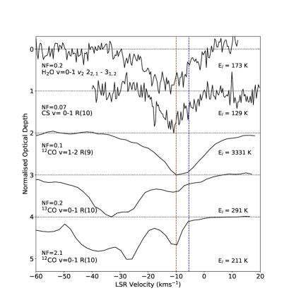
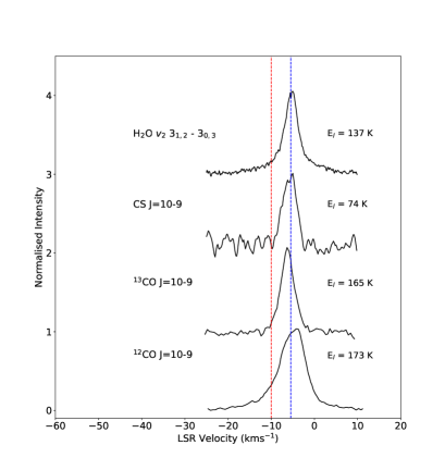
Figure 1: Comparison between IR and sub-mm line profiles. The IR lines are shown as optical depth profiles. The sub-mm profiles for CS, ¹³CO and ¹²CO are taken from Kaźmierczak-Barthel et al. (2014) and the sub-mm H₂O line is taken from Choi et al. (2015). The IR H₂O line is from our EXES data. The dashed red and blue lines indicate -10 kms^-1 and -5.5 kms^-1 respectively. Lines are normalised and lower energy levels given. For the IR lines, normalisation factors (NF) are given and horizontal baselines are shown.

The ¹²CO v=0-1 ro-vibrational lines are saturated up until J=9, and thus we have elected to focus here on the optically thin ¹³CO and ¹²CO v=1-2 transitions. All components in the ¹²CO v=0-1 line blend into one saturated line except for a broad high velocity component indicative of a high velocity outflow.¹²CO v=1-2 line profiles also show a single component at -10 kms^-1. The line parameters derived from the Gaussian fits are summarised in Table 1. The line widths have been de-convolved with the instrumental resolution.

The ¹³CO lines show complex profiles with multiple velocity components (Figure 1), one of which coincides in velocity with the CS lines and ¹²CO v=1-2 transitions. Two temperature components (hot and cold; see Figure 2) are observed at this velocity. For the hot component (high J), we adopted the CS line width but the line width for the cold component (low J) had to be reduced (to 4.1 kms^-1). Absorption by the narrower cold component overwhelms the contribution by the warm component at the lower J-levels.

Table 1: CS and CO line parameters. ${\Delta}v$ is the line FWHM, ${\tau}_{0}$ is the optical depth at line centre and N_l is the column density in the lower energy level of the transition, with energy E_l. A_ij is the Einstein A coefficient for the transition and g_l is the statical weight.

Species	Transition	Wavelength (${\mu}m$)	El (K)	gl	Aij (s-1)	$v_{lsr}$ (kms-1)	${\Delta}v$ (kms-1)	${\tau}_{0}$	Nl ($\times$1014 cm-2)
CS v=0-1	R(3)	7.8212	14.1	7	7.2	-11.9 $\pm 0.5$	8.3 $\pm 1.5$	0.031 $\pm 0.004$	1.9 $\pm 0.4$
	R(4) *	7.8116	23.5	9	7.4	-9.4 $\pm 0.5$	6.1 $\pm 1.3$	0.032 $\pm 0.004$	1.6 $\pm 0.4$
	R(5)	7.8020	35.3	11	7.6	-10.1 $\pm 0.5$	7.7 $\pm 1.3$	0.039 $\pm 0.004$	2.3 $\pm 0.5$
	R(7) *	7.7833	65.8	15	7.8	-10.4 $\pm 0.2$	6.4 $\pm 0.6$	0.056 $\pm 0.003$	3.0 $\pm 0.3$
	P(8)	7.9443	84.6	17	8.1	-10.9 $\pm 0.5$	9.6 $\pm 1.5$	0.055 $\pm 0.006$	4.5 $\pm 0.9$
	R(9)	7.7649	105.8	19	8.0	-9.5 $\pm 0.6$	11.2 $\pm 1.8$	0.051 $\pm 0.005$	4.1 $\pm 0.5$
	R(10)	7.7559	129.2	21	8.0	-11.1 $\pm 0.3$	10.4 $\pm 0.9$	0.061 $\pm 0.004$	4.7 $\pm 0.5$
	R(11)	7.7469	155.1	23	8.1	-12.1 $\pm 0.3$	9.9 $\pm 0.8$	0.060 $\pm 0.002$	4.4 $\pm 0.4$
	R(18)	7.6868	401.8	37	8.5	-12.0 $\pm 0.3$	11.0 $\pm 0.8$	0.063 $\pm 0.003$	5.0 $\pm 0.6$
	R(22) *	7.6545	594.5	45	8.7	-12.7 $\pm 0.4$	10.7 $\pm 1.2$	0.080 $\pm 0.004$	6.1 $\pm 2.4$
	R(23)	7.6467	648.5	47	8.8	-10.3 $\pm 0.9$	8.4 $\pm 3.8$	0.016 $\pm 0.003$	4.2 $\pm 1.1$
	R(24) *	7.6389	704.7	49	8.8	-5.2 $\pm 0.7$	15.0 $\pm 1.8$	0.060 $\pm 0.003$	5.9 $\pm 1.9$
	R(26)	7.6237	824.4	53	8.9	-8.4 $\pm 0.6$	7.9 $\pm 2.0$	0.048 $\pm 0.007$	3.0 $\pm 0.7$
	R(27) *	7.6162	887.8	55	9.0	-11.2 $\pm 0.6$	4.9 $\pm 1.2$	0.076 $\pm 0.006$	3.6 $\pm 0.8$
	R(28)	7.6088	953.4	57	9.0	-10.0 $\pm 0.4$	6.8 $\pm 1.0$	0.055 $\pm 0.008$	3.1 $\pm 0.7$
	R(29)	7.6015	1021.5	59	9.1	-10.9 $\pm 0.4$	6.7 $\pm 1.2$	0.078 $\pm 0.008$	4.4 $\pm 0.8$
	R(31) *	7.5871	1164.5	63	9.2	-8.0 $\pm 0.9$	11.4 $\pm 4.1$	0.024 $\pm 0.005$	1.8 $\pm 0.8$
	R(33)	7.5731	1316.8	67	9.2	-9.0 $\pm 0.6$	5.2 $\pm 1.5$	0.051 $\pm 0.009$	2.5 $\pm 0.7$
13CO v=0-1	P(1)	4.7792	5.2	6	32.4	-9.4 $\pm 0.2$	4.1	0.50 $\pm 0.04$	72.4 $\pm 7.3$
	P(2)	4.7877	15.8	10	21.5	-9.3 $\pm 0.1$	4.1	0.57 $\pm 0.02$	77.5 $\pm 3.6$
	R(2)	4.7463	15.8	10	14.2	-9.7 $\pm 0.3$	4.1	0.68 $\pm 0.07$	67.0 $\pm 8.0$
	R(3)	4.7383	31.7	14	14.8	-9.3 $\pm 0.1$	4.1	0.70 $\pm 0.02$	68.6 $\pm 2.7$
	P(3)	4.7963	31.7	14	19.3	-9.3 $\pm 0.2$	4.1	0.61 $\pm 0.04$	79.0 $\pm 6.2$
	P(4)	4.8050	52.8	18	18.2	-9.3 $\pm 0.2$	4.1	0.57 $\pm 0.03$	72.4 $\pm 5.2$
	R(5)	4.7227	79.3	22	15.5	-8.3 $\pm 0.2$	4.1	0.44 $\pm 0.06$	38.6 $\pm 5.7$
	R(6)	4.7150	111.0	26	15.8	-9.1 $\pm 0.3$	4.1	0.31 $\pm 0.06$	29.3 $\pm 5.9$
	R(9)	4.6927	237.9	38	16.4	-12.1 $\pm 0.7$	11.2	0.14 $\pm 0.01$	23.6 $\pm 3.1$
	P(9)	4.8501	237.9	38	16.4	-13.2 $\pm 0.8$	11.2	0.10 $\pm 0.01$	18.3 $\pm 2.6$
	R(10)	4.6853	290.8	42	16.5	-10.5 $\pm 0.6$	11.2	0.10 $\pm 0.01$	17.5 $\pm 2.5$
	R(11)	4.6782	349.0	46	16.7	-12.0 $\pm 0.5$	11.2	0.11 $\pm 0.01$	18.9 $\pm 2.3$
	P(11)	4.8689	349.0	46	16.1	-13.0 $\pm 0.6$	11.2	0.05 $\pm 0.01$	10.0 $\pm 1.8$
	R(12)	4.6711	412.3	50	16.8	-12.0 $\pm 0.6$	11.2	0.09 $\pm 0.01$	16.9 $\pm 1.9$
	R(13)	4.6641	481.1	54	16.9	-12.0 $\pm 0.4$	11.2	0.09 $\pm 0.01$	15.9 $\pm 1.4$
	R(16)	4.6437	718.8	66	17.3	-10.8 $\pm 0.5$	11.2	0.10 $\pm 0.01$	16.6 $\pm 1.8$
12CO v=1-2	R(6)	4.6675	3199.5	13	33.2	-9.6 $\pm 0.6$	17.9 $\pm 1.4$	0.102 $\pm 0.006$	13.1 $\pm 1.6$
	R(7)	4.6598	3237.9	15	33.7	-8.2 $\pm 0.7$	19.9 $\pm 1.9$	0.108 $\pm 0.008$	15.6 $\pm 2.6$
	R(8)	4.6522	3281.8	17	34.1	-9.1 $\pm 0.4$	18.3 $\pm 0.9$	0.124 $\pm 0.006$	16.4 $\pm 1.4$
	R(9)	4.6448	3331.0	19	34.4	-8.6 $\pm 0.4$	17.9 $\pm 0.9$	0.113 $\pm 0.005$	14.8 $\pm 1.2$
	R(17)	4.5887	3922.5	35	36.6	-8.5 $\pm 0.3$	16.6 $\pm 0.9$	0.104 $\pm 0.005$	12.7 $\pm 1.1$
	P(18)	4.8948	4020.9	37	31.7	-7.1 $\pm 0.3$	13.9 $\pm 0.9$	0.083 $\pm 0.004$	9.4 $\pm 0.9$
	P(19)	4.9054	4124.8	39	31.4	-9.9 $\pm 0.8$	14.6 $\pm 3.8$	0.010 $\pm 0.009$	12.0 $\pm 1.9$
	R(20)	4.5694	4234.4	41	37.2	-6.1 $\pm 0.5$	16.0 $\pm 1.2$	0.088 $\pm 0.005$	10.3 $\pm 1.5$

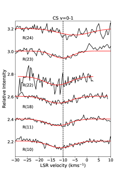
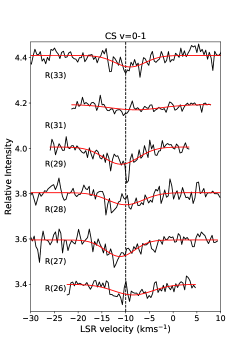
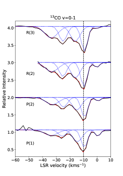
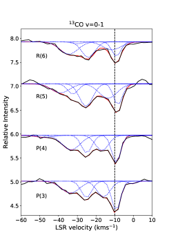
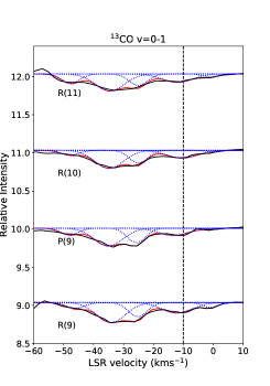
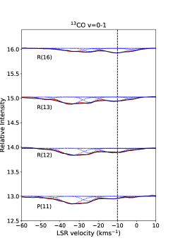
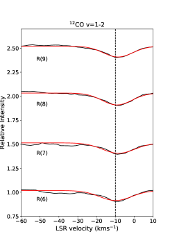
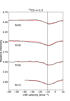
Figure 3: All lines of CS, ¹³CO and ¹²CO v=1-2. The blue dotted lines represent the individual velocity components and the red solid lines show the overall fit. The black dashed line denotes -10 kms^-1.

The detected, unblended lines of CS and CO are presented in Figure 3 in the Appendix. There is a spread in centroid velocity for a given species. The line widths for CS and hot ¹³CO are in agreement for equivalent energy level.

The rotation diagrams of CS, ¹³CO and ¹²CO v=1-2 are shown in Figure 2. In all cases the rotation diagrams are straight lines indicating that local thermodynamic equilibrium (LTE) is a good approximation. We have calculated the vibrational excitation temperature of ¹²CO from the v=1-2 transitions and the warm ¹³CO column density assuming a ¹²CO/¹³CO abundance ratio of 60 (Wilson & Rood, 1994). The derived vibrational excitation temperature of 625$\pm$56 K agrees well with a similar estimate by Mitchell et al. (1989). The similar values for the rotational and vibrational temperatures suggest vibrational LTE.

The excitation temperature and velocity for all three species (CS, ¹³CO high J and ¹²CO v=1-2) are very similar. This supports an origin in the same region. The physical conditions for the detected species are summarised in Table 2. An estimate of the column density of hot ¹²CO from the lines of vibrationally excited ¹²CO gives 1.5$\pm$0.6$\times$10¹⁸ cm^-2. We derive an upper limit on CS in the -33 kms^-1 velocity component of $<$ 8$\times$10¹⁴ cm^-2.

Table 2: Summary of Molecular Species in AFGL 2591

Species	$v_{lsr}$ (kms-1)	Tex (K)	N ($\times$1016cm-2)	N/N(12CO)1
CS v=0-1	-10 $\pm$0.5	714 $\pm$59	1.6 $\pm$0.1	8.0$\times$10-3
12CO v=1-2	-8.4 $\pm$0.5	664 $\pm$43	1.48 $\pm$0.6	7.4$\times$10-3
13CO v=0-1	-11.95 $\pm$0.6	670 $\pm$124	3.4 $\pm$0.4	0.02
H2O2	-11 $\pm$0.3	640 $\pm$80	370 $\pm$80	1.85
13CO v=0-1	-9.2 $\pm$0.2	47 $\pm$3	3.8 $\pm$0.2	0.02
13CO v=0-1	-33 $\pm$0.8	76 $\pm$10	3.4 $\pm$0.2	0.02
13CO v=0-1	-33 $\pm$0.5	244 $\pm$11	5.9 $\pm$ 0.4	0.03
CS v=0-1	-33 $\pm$0.5	244 $\pm$11	$<$ 0.08	$<$ 2.2$\times$10-4

3.2 CS and CO: Infrared vs Submillimeter

From our observations we derive a different systemic velocity than from sub-mm studies of AFGL 2591 (Figure 1) in both CS, ¹³CO and ¹²CO v=1-2 (-10 kms^-1 compared to -5.5 kms^-1, Bally & Lada1983). van der Tak et al. (1999) studied AFGL 2591 at sub-mm, radio and IR wavelengths, at lower resolution, and derive a centroid velocity for ¹³CO absorption of -5.5 kms^-1, in agreement with the systemic velocity of rotational emission lines, including CS (Boonman et al., 2001; Benz et al., 2007; Kaźmierczak-Barthel et al., 2014). However their IR transitions show a spread in velocity of -3.5 to -12.4 kms^-1 which they attribute to atmospheric interference, picking only a few lines to derive their value of -5.5 kms^-1.

The intrinsic line widths that we observed are broader than for sub-mm studies (Figure 1). As an example, the CS J=10-9 transition has a width of 3.5 kms^-1 whereas our CS rovibrational transition v=0-1 R(10) has a width of 10.4 kms^-1. The H₂O 3(1,2)-3(0,3) line has a width of 3.1 kms^-1 in the sub-mm compared to 16.5 kms^-1 for the ${\nu}_{2}$=0-1 2(2,1)-3(1,2) IR line.

We suggest our higher temperature, higher velocity IR observations trace more turbulent gas closer to the central source, probing deep into the base of the outflow, whereas sub-mm observations trace more extended gas at the velocity of the quiescent envelope.

The CS, ¹³CO v=0-1 and ¹²CO v=1-2 temperatures are very similar and given the difference in critical densities, suggest gas in LTE. The critical densities for J=7-6 are 2$\times$10⁵ cm^-3 (Yang et al., 2010) and 3$\times$10⁷ cm^-3 (Turner et al., 1992) for CO and CS respectively. Therefore we estimate that the density must exceed 10⁷ cm^-3 in order to maintain LTE. The critical density of ¹²CO v=1-2 cannot be used due to the high optical depth of the ¹²CO v=0-1 transitions, which may lead to line trapping and tends to increase the vibrational excitation temperature.

Assuming a ¹²CO/H₂ abundance of 2x10^-4 (Lacy et al., 1994) and constant density of 10⁷ cm^-3, we derive a physical size for the absorbing region of $<$ 130 AU. At a distance of 3.3 kpc (Rygl et al., 2012) this corresponds to $<$0.04^′′.

The velocity structure of the inner region (down to 500 AU) of the hot core in AFGL 2951 has been well resolved and modelled by Wang et al. (2012). A high velocity gradient is found for SO₂ and the velocity field of the blue shifted component is observed to have the highest negative velocities towards the centre on the source. However the highest velocity that is reached is $\sim$ -7 kms^-1, at the very centre. This further indicates that CS at -10 kms^-1 would not be observed at sub-mm wavelengths. Combined with the fact that SO₂ is a molecular tracer for shocks or outflows (Schilke et al., 1997), Wang et al. (2012) conclude that the SO₂ emission originates in an interactive layer between the upper parts of a disk-like structure and the outflow.

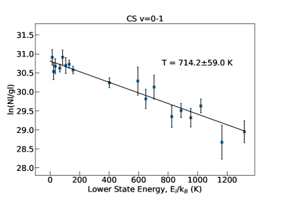
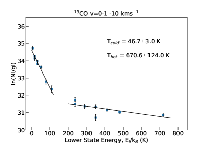
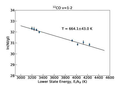
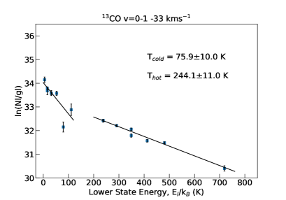
Figure 2: CS and CO rotation diagrams. Temperatures for each species are shown, with two temperature components for ¹³CO.

van der Tak et al. (1999) conclude that the outflow of AFGL 2591 points towards us along the line of sight. In order to explain CS (7-6) emission, Bruderer2009proposethattheirobservationstracedensewallsoftheoutflow; atavelocityofaround-5.5kms$^-1$. Given that the extreme velocities originate in the centre of the source, and that our EXES observations show an average velocity around -10 kms^-1, we propose that we are looking into the outflow, probing deeply towards the protostar to the base of the outflow. Also the broad line profiles of CS are indicative of a shocked region. The high temperature implies that the gas lies close to the protostar, further supporting the proposed origin as the base of the outflow.

3.3 Chemistry of CS

We derive a CS/¹²CO abundance of 8x10^-3 and CS/H₂ abundance of 2$\times$10^-6, assuming a CO/H₂ ratio of 2$\times$10^-4. This abundance is two orders of magnitude higher than sub-mm observations of the hot core and envelope (van der Tak et al., 2003; Jiménez-Serra et al., 2012). This, once again, illustrates that the IR observations probe a very different region in this source. Consequently hot CS contains 6$\pm$0.8 % of the cosmic sulphur budget, assuming an S/H ratio of 1.3$\times$10^-5. Compared to the Orion Hot Core which has a CS/CO abundance of 4.1$\times$10^-4 derived from sub-mm observations (Tercero et al., 2010), the CS abundance in the gas traced by the IR observations of the hot core in AFGL 2591 is much higher.

Chemical models based on sub-mm observations (Charnley et al., 1997; Doty et al., 2002) derive a CS abundance of the order 1$\times$10^-8 with respect to H₂. A two phase, time-dependent gas-grain model (Viti et al., 2004) has been used to study the sulphur chemistry in the Orion Hot Core, and predicts the abundance of CS as a function of hot core age (Esplugues et al., 2014). The first and second phase simulate depletion onto, and sublimation from, grain surfaces respectively. For a hot core with a mass of 10 M_⊙, solar sulphur abundance and a density of 10⁷ cm^-3, a CS/CO abundance of around 5$\times$10^-3 is achieved after 6$\times$10⁴ yr.

The abundances of CS, H₂CS and SO₂ increase such that these species become the most abundant sulphur-bearing molecules for an evolved hot core (Esplugues et al., 2014). The main chemical pathway that is responsible for the production of CS in this model is CH₂ + S $\rightarrow$ CS + H₂. Chemical models predict large amounts of atomic sulphur at high temperatures (Doty et al., 2002). This arises due to abstraction of H₂S which is efficient at high temperatures. At the same time small hydrocarbons are formed by the breakdown of CO via cosmic ray ionisation.

Therefore we propose two scenarios to interpret the CS abundance. The first is that AFGL 2591 is a more evolved hot core in which all sulphur is converted to H₂S on grain surfaces, and then converted back to S in the gas-phase after ice mantle sublimation. Then, at long timescales, enough CS is produced in the hot inner region of the hot core to explain our observations (Esplugues et al., 2014). These models are not optimised to AFGL 2591 which would likely have an effect on the CS abundance, therefore a more in depth study using chemical models would be necessary to clarify the proposed timescales. We note that H₂S ice has not been observed in absorption towards massive protostars (Smith, 1991) at abundance upper limits a factor of 7 lower than that of CS, putting H₂S as a source of the gas phase S into question. Deeper searches for H₂S would be very helpful to asses the sulphur budget in interstellar ices.

The alternative scenario is that our observations trace a disk-wind interaction zone very close to the protostar. In this case the cosmic ray ionisation rate would be high, which would favour the breaking of C out of CO, which could lead to the enhancement of CS production. Again, atomic sulphur is produced via abstraction of H₂S. May et al. (2000) find that grain sputtering becomes important in shocks around 15 kms^-1, therefore sulphur could also be released from grain mantles in the presence of shocks.

The conditions and chemical history of AFGL 2591 are clearly favourable for the production of CS. A high CS/CO abundance of 7$\pm 0.4$$\times$10^-3 has also been observed at MIR wavelengths in NGC 7538 IRS 1 (Knez et al., 2009) with TEXES. Nevertheless, the enhanced CS abundance is still not enough to appoint this molecule as the main reservoir of sulphur in hot cores. A high abundance of warm SO₂ has also been observed with EXES in the hot core Mon R2 IRS 3. (Dungee et al., submitted to ApJL). This also is not observed in the sub-mm suggesting that a large amount of sulphur is visible only at IR wavelengths.

4 Conclusions

We present the first detection of ro-vibrational transitions of CS in the hot core of AFGL 2591 with EXES. The CS observations are complemented with high resolution iSHELL CO observations. The CO gas is found to have five velocity components, one of which is consistent with the velocity of CS, -10 kms^-1. ¹²CO v=1-2 is also observed at this velocity. A temperature of 714$\pm 59$ K is derived from the rotation diagram of CS, and the observation of CS up to J level of 33, along with a similar excitation temperature for the pure rotational CO lines, imply high densities ($>10^{7}$ cm^-3). The temperature is consistent with hot ¹³CO and ¹²CO v=1-2 which have 670$\pm 124$ K and 664$\pm 43$ K respectively.

The systemic velocity of AFGL 2591 that we derive is 5 kms^-1 bluer than that derived from sub-mm observations. We propose that this is because we are observing the base of the blue-shifted outflow very close to the central IR source. This is reflected in the high densities and temperatures derived in our observations.

The abundance of CS observed to be 8x10^-3 and 2$\times$10^-6 with respect to CO and H₂ respectively. This is two orders of magnitude above what is derived from sub-mm observations, 1$\times$10^-8 with respect to H₂. This provides evidence of a large sulphur depository which is detectable more readily at IR wavelengths. IR observations are sensitive to a different region of the hot core than sub-mm observations. IR observations of CS trace gas in the hot core that is much hotter and denser than do sub-mm observations, and that is at a larger systemic velocity. Therefore they probe much deeper into the innermost parts of the hot core, avoiding any contamination by the surrounding envelope.

Chemical models support the derived abundance of CS if AFGL 2591 is an evolved hot core. Alternatively our observations may be tracing the onset of a disk wind at the base of the outflow.

5 Appendix

References

- Bally & Lada (1983) Bally, J., Lada, C. J. 1983, ApJ, 265, 824
- Benz et al. (2007) Benz, A. O., Staüber, P., Bourke, T. L., van der Tak, F. F. S., et al. 2007, A&A, 475, 549
- Beuther et al. (2007) Beuther, H., Churchwell, E. B., McKee, C. F., & Tan, J. C. 2007, Protostars and Planets V, 165
- Boonman et al. (2001) Boonman, A. M. S., Stark, R., van der Tak, F. F. S., et al. 2001, ApJ, 553, L63
- Blake et al. (1987) Blake, G. A., Sutton, E. C., Masson, C. R., & Phillips, T. G. 1987, ApJ, 315, 621
- Bruderer et al. (2009) Bruderer, S., Benz, A. O., Bourke, T. L., & Doty, S. D. 2009, A&A, 503, L13
- Carr et al. (1995) Carr, J. S., Evans, N. J., Lacy, J. H., & Zhou, S. 1995, ApJ, 450, 667
- Ceccarelli (2008) Ceccarelli, C. 2008, Organic Matter in Space Proceedings IAU Symposium, No. 251, 2008, S. Kwok & S. Sandford, eds.
- Cesaroni et al. (2005) Cesaroni, R. 2005, in IAU Symp. 227, Massive Star Birth: A Crossroads of Astrophysics, ed. R. Cesaroni, M. Felli, E. Churchwell, & M. Walmsley (Cambridge: Cambridge Univ. Press), 59
- Charnley et al. (1997) Charnley, S. B. 1997, ApJ, 481, 396
- Choi et al. (2015) Choi, Y., van der Tak, F. F. S., van Dishoeck, E. F., Herpin, F., & Wyrowski, F. 2015, A&A, 576, A85
- Clarke et al. (2015) Clarke, M., Vacca, W. D., & Shuping, Y. S. 2015, Astronomical Data Analysis Software and Systems: XXIV ASP Conference Series, Vol. 495
- Cushing et al. (2004) Cushing, M. C., Vacca, W. D., & Rayner, J. T. 2004, PASP, 116, 362
- Doty et al. (2002) Doty, S. D., van Dishoeck, E. F., van der Tak, F. F. S., & Boonman, A. M. S. 2002, A&A, 389, 446
- Esplugues et al. (2014) Esplugues, G. B., Viti, S., Goicoechea, J. R., & Cernicharo, J. 2014, A&A, 567, A95
- Gordon et al. (2017) Gordon, I. .E., Rothman, L. S., Hill, C. et al. 2017, JQSRT, 203, 3
- Hatchell et al. (1998) Hatchell, J., Thompson, M. A., Millar, T. J., et al. 2009, A&A, 504, 853
- Indriolo et al. (2015) Indriolo, N., Neufeld., D. A., DeWitt, C. N., Richter, M. J., et al. 2015, ApJ, 802: L14
- Jiménez-Serra et al. (2012) Jiménez-Serra, I., Zhang, Q, Viti, S., Martín-Pintado, J., & De-Wit, W. -J. 2012, ApJ, 753, 34
- Kaźmierczak-Barthel et al. (2014) Kaźmierczak-Barthel, M., van der Tak, F. F. S., Helmich, F. P., et al. 2014, A&A, 567, A53
- Keane et al. (2001) Keane, J. V., Boonman, A. M. S., Tielens, A. G. G. M., et al. 2001, A&A, 376, L5
- Knez et al. (2009) Knez, C., Lacy, J. H., Evans, N. J., van Dishoeck, E. F., & Richter, M. J. 2013, ApJ, 696, 471
- Kurtz et al. (2000) Kurtz, S., Cesaroni, R., Churchwell, E., Hofner, P., & Walmsley, C. M. 2000, in Protostars and Planets IV, ed. V. Mannings, A. P. Boss, & S. S. Russell (Tucson, AZ: Univ. Arizona Press), 299
- Lacy et al. (1991) Lacy, J. H., Carr, J. S., Evans, N. J., Baas, F., Achtermann, J. M., & Arens, J. F. 1991, ApJ, 376, 556
- Lacy et al. (1994) Lacy, J. H., Knacke, R., Geballe, T. R., Tokunaga, A. T. 1994, ApJ, 428, L69
- Lacy et al. (2002) Lacy, J. H., Richter, M. J., Greathouse, T. K., Jaffe, D. T., & Zhu, Q. 2002, PASP, 114, 153
- Li et al. (2015) Li, J., Wang, J., Zhu, Q., Zhang, J., & Li, D. 2015, ApJ, 802, 40
- May et al. (2000) May, P. W., Pineau des Forêts, G., Flower, D. R., et al. 2000, MNRAS, 318, 809
- Mitchell et al. (1989) Mitchell, G. F., Curry, C., Maillard, J., & Allen, M. 1989, ApJ, 341, 1020
- Mitchell et al. (1990) Mitchell, G. F., Maillard, J. P., Allen, M., Beer, R., & Belcourt, K. 1990, ApJ, 363, 554
- Plambeck & Wright (1987) Plambeck, R. L., & Wright, M. C. H. 1987, ApJ, 317, L101
- Rayner et al. (2016) J. T. Rayner, A. Tokunaga, D. Jaffe, M. Bonnet, G. Ching, M. Connelley, D. Kokubun, C. Lockhart, & E. Warmbier. 2016, SPIE, 9908E, 84R
- Richter et al. (2010) Richter, M. J., Ennico, K. A., McKelvey, M. E., & Seifahrt, A. 2010, in Society of Photo-Optical Instrumentation Engineers (SPIE) Conference Series, Vol. 7735
- Rygl et al. (2012) Rygl K. L. J. et al. 2012, A&A, 539, 79
- Schilke et al. (1997) Schilke, P., Groesbeck, T. D., Blake, G. A., & Phillips, T. G. 1997, ApJS, 108, 301
- Smith (1991) Smith, R. G. 1991, MNRAS, 249, 172
- Tercero et al. (2010) Tercero, B., Cernicharo, J., Pardo, & J. R., Goioechea, J. R. 2010, A&A, 517, A96
- Tieftrunk et al. (1994) Tieftrunk, A., Pineau Des Forêts, G., Schilke, P., et al. 1994, A&A, 289, 579
- Turner et al. (1992) Turner, B. E., Chan, K., Green, S., & Lubowich, D. A. 1992, ApJ, 399, 114
- van Dishoeck & Blake (1998) van Dishoeck, E. F., & Blake, G. A. 1998, ARA&A, 36, 317
- van der Tak et al. (1999) van der Tak, F. F S., van Dishoeck, E. F., Evans, N. J., & Bakker, E. J. 1999, ApJ, 522, 991sub-mm
- van der Tak (2003) van der Tak, F. F. S. 2003, Star Formation at High Angular Resolution ASP Conference Series, Vol. S-221, R. Jayawardhana, M. G. Burton, & T. L. Bourke
- van der Tak et al. (2003) van der Tak, F. F. S., Boonman A. M. S., Braakman, R., & van Dishoeck, E. F. 2003, A&A, 412, 133
- Villanueva et al. (2018) Villanueva, G. L., Smith, M. D., Protopapa, S., Faggi, S., & Mandell, A. M. 2018, J. Quant. Spec. Radiat. Transf., 217, 86
- Viti et al. (2004) Viti, S., Collings, M. P., Dever, J. W., McCoustra, M. R. S., & Williams, D. A. 2004, MNRAS, 354, 1141
- Wang et al. (2012) Wang, K. S., van der Tak, F. F. .S., & Hogerheijde, M. R. 2012, A&A, 543 A22
- Wilson & Rood (1994) Wilson, T. L., & Rood, R. T. 1994, ARA&A, 32, 191
- Yang et al. (2010) Yang, B. ., Stancil, P. C., Balakrishnan, N., & Forrey, R. C. 2010, ApJ, 718, 1062
- Young et al. (2012) Young, E. T., Becklin, E. E., Marcum, P. M., et al. 2012, ApJ, 749, L17