Joint modelling of progression-free and overall survival and computation of correlation measures

Abstract

[Summary]In this paper we derive the joint distribution of progression-free and overall survival as a function of transition probabilities in a multistate model. No assumptions on copulae or latent event times are needed and the model is allowed to be non-Markov. From the joint distribution, statistics of interest can then be computed. As an example, we provide closed formulas and statistical inference for Pearson’s correlation coefficient between progression-free and overall survival in a parametric framework. The example is inspired by recent approaches to quantify the dependence between progression-free survival, a common primary outcome in phase III trials in oncology, and overall survival. We complement these approaches by providing methods of statistical inference while at the same time working within a much more parsimonious modelling framework. Our approach is completely general and can be applied to other measures of dependence. We also discuss extensions to nonparametric inference. Our analytical results are illustrated using a large randomized clinical trial in breast cancer.

, , and (xxxx), Joint modelling of progression-free and overall survival and computation of correlation measures, Stat Med, xxxx;xx:x–x.

1 Introduction

An established way to evaluate performance of therapies in clinical trials are time-to-event endpoints. While overall survival (OS) remains the gold standard for demonstrating clinical benefit, especially in oncology, alternative endpoints such as progression-free survival (PFS), are also accepted by Health Authorities^{1, 2}. PFS is not only considered a surrogate for OS, but may provide clinical benefit by itself, e.g. by delaying symptoms or subsequent therapies ³. Further advantages of the use of PFS are shorter trial durations and the fact that, as opposed to OS, PFS is not confounded by the use of later line, i.e. post-progression, therapies, and PFS is less vulnerable to competing causes of death than OS⁴.

Methodology has been developed to assess surrogacy of one endpoint for another⁵ and these methodologies have been applied to a wide range of indications⁶. One important aspect in the assessment of surrogacy is to quantify the correlation between the surrogate and the real endpoint⁷. This aspect has received quite some attention in the literature lately^{8, 9}. These two papers consider Pearson’s correlation coefficient and rely on an illness-death model without recovery (IDM) to model the association between PFS and OS. To specify the underlying statistical model for the likelihood function for parametric estimation, they use a latent failure time approach. One characteristic of the latent failure time approach is that it allows for PFS events after OS, see Section 2.3. Within this model formulation, Fleischer et al.⁸ then derive closed formulas for the survival functions $S_{PFS}$ and $S_{OS}$ for PFS and OS as well as the correlation coefficient $\mathop{\rm Corr}\nolimits({\rm PFS},{\rm OS})$ by assuming an exponential distribution for all transition intensities in the underlying multistate model. Li and Zhang⁹ generalized these results to Weibull transition intensities, where closed formulas are provided imposing the assumption of equal Weibull shape parameter for all three transition intensities.

Notably, while in Fleischer et al.⁸ and Li and Zhang⁹ point estimates are provided for the quantities of interest based on the made parametric assumptions, they do not provide a discussion of statistical inference, e.g. how to derive pointwise confidence intervals for the distribution functions at a milestone time or for the correlation coefficient directly. We further discuss the contributions of these papers in detail in Section 4. One aim of this paper is to provide for such methods of statistical inference while ensuring that PFS does not exceed OS.

Finally, in a Bayesian framework the joint distribution of PFS and OS can be modelled based on a Gaussian copula¹⁰. Inference is based on a likelihood function that relies on the latent failure time approach, i.e. derives each patient’s contribution to the likelihood based on his or her censoring pattern.

We extend the existing body of work in multiple directions. To begin, we model PFS and OS as arising from an IDM without recovery. The only assumption will be that the model is smooth in the sense that transition intensities between all states of the model exist. No assumption about latent times or copulas will be made and the model is allowed to be non-Markov. Because the transition probabilities provide a full description of the IDM, we first recollect closed formulas for the transition probabilities in an IDM process $X$, following Hougaard ¹¹. We derive these probabilities for $X$ a general, not necessarily Markov, process. The implication of $X$ being non-Markov for the considered IDM is that the hazard for the transition from the diseased into the death state, $\alpha_{12}(t;{t_{1}})$, will depend on the time $t$ since time origin and on the time ${t_{1}}$ of entry into the diseased state. While conceptually offering more modelling flexibility, this generalization complicates derivation of closed formulas for the quantities of interest, since one additionally needs to integrate out over the distribution of ${t_{1}}$. There are multiple ways how $\alpha_{12}(t;{t_{1}})$ can depend on ${t_{1}}$, e.g. as function of $t$ and ${t_{1}}$ separately or via the duration $t-{t_{1}}$ only. Naming of these specific assumptions has not been unambiguously in the literature and we provide a discussion of the terminology.

Based on the transition probabilities, we derive closed formulas not only for $S_{PFS}$, $S_{OS}$, and $\mathop{\rm Corr}\nolimits({\rm PFS},{\rm OS})$, but also for the joint distribution of ${\rm PFS}$ and ${\rm OS}$. It is worth noting that the latter entirely specifies the association between PFS and OS based on the assumed IDM model alone, i.e. without having to make additional assumptions, e.g. about a copula function as in Burzykowski et al.⁵. For all these quantities, and under parametric assumptions on the transition hazards, statistical inference can be performed either via standard likelihood theory together with the $\delta$-rule or bootstrap for parametric models. Note that, unlike in Li and Zhang⁹, with the IDM formulation there is no need to restrict the Weibull shape parameter to coincide between all three transition intensities.

There is a rich theory allowing for nonparametric estimation of transition hazards and subsequently probabilities, see e.g. Hougaard ¹¹ or Aalen et al.¹². Through simple plug-in of these estimates we also get nonparametric estimates for the above quantities, thereby extending the existing purely parametric approaches^{8, 9}. Inference for these models is possible via bootstrap. Estimating transition probabilities nonparametrically based on possibly right-censored data adds one complication though: to estimate a correlation coefficient we rely on expectations and variances with respect to $S_{PFS}$ and $S_{OS}$, i.e. we either need estimates of these survival functions down to 0 or we restrict estimation of expectations to some maximum time.

It is well-known that the latent failure formulation of competing risk or multistate models in general suffers from identifiability and interpretability issues. We discuss these in more detail and shed some light on how the latent times, if they are introduced, relate to the transition hazards from an IDM. In contrast to using latent times, copulas may be applied to modelling the dependence of PFS and OS without assuming such a latent structure. However, typical copula models consider the dependence of general multivariate survival times, such as the lifetimes of twins, and neither allow for PFS $=$ OS with positive probability nor ensure the natural PFS $\leq$ OS. These two aspects are accounted for in a multistate model, which makes the latter framework a natural choice for joint modelling of PFS and OS.

Lately, Weber and Titman¹³ also pointed out the mentioned deficiencies of copulas and the latent-failure time model used in ^{8, 9} to model the association between PFS and OS. They also advocate an IDM, but, in contrast to our paper, focus on demonstrating the shortcomings of copula modelling for PFS and OS using Kendall’s $\tau$, also using the likelihood approach of Li and Zhang⁹.

We would like to emphasize that our results are neither specific to the modelling of PFS and OS in oncology nor to investigating their correlation as one choice of measuring dependence, but are applicable to any IDM.

In Section 2 we introduce a multistate model that allows to explicitly derive the joint distribution of PFS and OS under virtually no assumptions and we show how this can be used to derive a formula for Pearson’s correlation coefficient. Furthermore, we outline that patient trajectories for PFS and OS from our model can easily be simulated. Section 3 revisits existing approaches using the latent failure time approach and discusses how our proposal allows to extend these methods using more parsimonious assumptions. How to make inference in our proposed setup is described in Section 4 while Section 5 reports on a small simulation study for the correlation coefficient; additional simulation results are provided in the online supplement. In Section 6 we then illustrate the developed methodology using a large Phase 3 randomized oncology clinical trial and compare it to previously proposed approaches. We conclude with a discussion in Section 7.

2 A multistate model for PFS and OS

We introduce the general model in Section 2.1 along with an algorithm to generate data from the model, which can, e.g., be used for numerical approximations. The model may or may not be time-inhomogeneous Markov, and violations of the Markov assumption are summarized in Section 2.2. Section 2.3 discusses advantages of our approach over latent failure time and over copula modelling. We also discuss how to derive the model specification within a latent times approach as in Fleischer et al.⁸ and Li and Zhang⁹ based on our more parsimonious model. Both transition probabilities of the multistate model and the joint distribution of PFS and OS are in Section 2.4. Based on the joint distribution, dependency measures of PFS and OS can be expressed, and we exemplarily consider the correlation in Section 2.5. We reiterate that our derivations hold for a general IDM without recovery. The model is not required to be Markov, the transition intensities may be time-dependent and their parametric specification may depart from those in Fleischer et al.⁸ and Li and Zhang⁹. Dependence measures other than Pearson’s correlation coefficient can be expressed, e.g. transition intensities can be plugged into (10) in Weber and Titman¹³ to receive Kendall’s $\tau$.

2.1 The general model and generation of PFS-OS trajectories

We jointly model progression and death in an ‘illness-death’ multistate model ^{14, 15}. The model is illustrated in Figure 1.

Figure 1: Multistate model for PFS and OS: PFS is the waiting time in the initial state $0$, OS is the waiting time until absorption in state $2$.

Let $X(t)$ denote the state occupied at time $t$, $t\geq 0$, $X(t)\in{\cal{S}}:=\{0,1,2\}$. We assume that all individuals are in the initial state $0$ at time $0$, $P(X(0)=0)=1$, typically upon randomization to treatment. At the time of diagnosis of progression, patients make a $0\to 1$ transition, and subsequent death is modelled as a $1\to 2$ transition. Patients who die without prior progression diagnosis make a direct $0\to 2$ transition into the absorbing state. Progression-free survival is the waiting time in the initial state $0$,

$${\rm PFS} = \inf\{t\,:\,X(t)\neq 0\},$$

and overall survival is the time until reaching the death state $2$,

$${\rm OS} = \inf\{t\,:\,X(t)=2\}.$$

Patients with a diagnosed progression have ${\rm PFS}<{\rm OS}$, while patients who make a direct $0\to 2$ transition have ${\rm PFS}={\rm OS}$. At this stage, it is important to note that no assumption about any dependence or independence of PFS and OS has entered so far, other than the natural ${\rm PFS}\leq{\rm OS}$. That is, the only assumption we have made so far is that there is no progression after death. We will assume that the multistate model is sufficiently smooth in that the following intensities exist,

$$\alpha_{0j}(t)=\lim_{\Delta t\searrow 0}\frac{P({\rm PFS}\in[t,t+\Delta t),X({\rm PFS})=j\,|\,{\rm PFS}\geq t)}{\Delta t},\,j=1,2,$$ (1)

and, for ${t_{1}}<t$,

$$\alpha_{12}(t;{t_{1}}) = \lim_{\Delta t\searrow 0}\frac{P(X(t+\Delta t)=2\,|\,X(t-)=1,{\rm PFS}={t_{1}})}{\Delta t}$$

$$= \lim_{\Delta t\searrow 0}\frac{P({\rm OS}-{\rm PFS}\in[t-{t_{1}},t-{t_{1}}+\Delta t)\,|\,{\rm OS}\geq t,{\rm PFS}={t_{1}})}{\Delta t}.$$

These definitions are generally valid, also for $X(t)$ a non-Markov process. In Section 2.2 we discuss the classification of assumptions on $X$ and the implications for the definition of $\alpha_{12}$ in more detail.

The waiting times in the initial state and in the intermediate state in the model of Figure 1 have survival distributions

$$S_{PFS}(t)\ =\ P({\rm PFS}>t)\ =\exp\left(-\int_{0}^{t}\alpha_{01}(u)+\alpha_{02}(u){\rm\;d}u\right)$$ (3)

and, conditional on progression at time $t_{1}$,

$$P({\rm OS}-{\rm PFS}>v\,|\,{\rm PFS}={t_{1}}<{\rm OS}) = \exp\left(-\int_{t_{1}}^{{t_{1}}+v}\alpha_{12}(u;{t_{1}}){\rm\;d}u\right).$$ (4)

Noting that ${\rm PFS}<{\rm OS}$ given ${\rm PFS}={t_{1}}$ with probability $\alpha_{01}({t_{1}})/(\alpha_{01}({t_{1}})+\alpha_{02}({t_{1}}))$ ¹⁶, these formulae can be used to simulate PFS-OS-trajectories ¹⁵ without resorting to latent times. One first simulates a PFS time using Equation (3), say ${\rm PFS}={t_{1}}$. In a second step, one decides on ${\rm PFS}<{\rm OS}$, if a binomial experiment with ‘success’ probability $\alpha_{01}({t_{1}})/(\alpha_{01}({t_{1}})+\alpha_{02}({t_{1}}))$ yields ‘success’. In this case, the residual time until OS is simulated from Equation (4). Otherwise, ${\rm PFS}={\rm OS}$. This simulation approach is advantageous for numerical approximations. Below, we will find that some expressions may be rather tedious in the general non-Markov case, but they may be simply approximated by their empirical counterparts after having generated a large number of trajectories.

2.2 Assumptions for non-Markov models

In a non-Markov IDM, i.e., without the possibility of $1\to 0$ transitions, and common initial state 0, the $1\to 2$ hazard $\alpha_{12}(t;{t_{1}})$ will depend on time $t$ since time origin and on time ${t_{1}}$ of entry into state 1, see Chapter 5 in Hougaard¹¹ or Chapter 12 in Beyersmann et al.¹⁵. Since all transitions other than $1\to 2$, i.e. $0\to 1$ and $0\to 2$, are rooted in 0, making the transition intensity $\alpha_{12}(t;{t_{1}})$ depend on ${t_{1}}$ summarizes the entire “past” prior to the $1\to 2$ transition.

Now, classification of non-Markov models does not seem to be entirely consistent in the literature. A model for which $\alpha_{12}(t;{t_{1}})$ depends only on the time since progression, $\alpha_{12}(t;{t_{1}})=\alpha_{12}(t-{t_{1}})$ for all ${t_{1}}<t$, goes by the name semi-Markov in Hougaard (Table 6.1)¹¹ and Beyersmann et al. (p. 229)¹⁵, or clock reset in Putter et al.¹⁷. The latter refers to the fact that the clock is re-set for the death hazard for patients that progressed. Andersen and Pohar Perme¹⁸ and Andersen¹⁹ refer to this model as homogeneous semi-Markov and to a model that depends on both $t$ and $t-t_{1}$, i. e. $\alpha_{12}(t;{t_{1}})=\alpha_{12}(t;t-{t_{1}})$, as semi-Markov. Equivalently, the general model, $\alpha_{12}(t;{t_{1}})=\alpha_{12}(t;{t_{1}})$, is denoted general Markov extension model¹¹ and simply non-Markov model¹⁵.

If the intensities are time-constant, $\alpha_{ij}(t)=\alpha_{ij}$, the model is (time-) homogeneous Markov. Note that $X(t)$ being homogeneous Markov always implies exponential transition intensities and vice-versa, see p. 465 in Aalen et al.¹² or p. 31 in Beyersmann et al.¹⁵.

2.3 Advantages of the multistate modelling approach

In the literature, it is not uncommon that PFS and OS are modelled as arising from latent failure times ^{20, 21, 8, 22, 23, 9, 24, 25}. Another approach is to use copulas to capture the dependence between PFS and OS ^{5, 26, 27, 10, 28}. Neither latent times nor copulas have been used in our general model of Section 2.1, and this is a conceptual advantage of the multistate modelling framework. To begin, copulas are a convenient method to model general bivariate survival data, e.g., lifetimes of twins, but the structure at hand is more specific: Firstly, PFS is always less than or equal to OS, but copulas do not place such a restriction on the pair of event times. This is meaningful for general bivariate survival data, but not for the ordered pair $(\mbox{PFS},\mbox{OS})$. Secondly, PFS $=$ OS with positive probability. However, in a copula model with continuous ‘marginal’ survival functions for PFS and OS, this will happen with probability zero only. Again, this is meaningful for general bivariate survival data, but not for $(\mbox{PFS},\mbox{OS})$, where PFS $=$ OS simply encodes that the waiting time in the intial state equals the waiting time until the terminal state.

For discussion of the latent failure time model, assume that there are latent, non-negative random variables $L_{1}$ and $L_{2}$ such that progression occurs, if $L_{1}<L_{2}$ (and then ${\rm PFS}=L_{1}$ and ${\rm OS}=L_{2}$). If, however, $L_{2}\leq L_{1}$, the patient dies without prior progression (and then ${\rm OS}=L_{2}$). There are two problems with this approach, the first of which may appear to be the more serious one, because it seemingly complicates estimating the correlation or the joint distribution of PFS and OS, but it really is the second problem that stands out: Firstly, it is well known from the competing risks literature²⁹ that one cannot tell from the observable data whether or not $L_{1}$ and $L_{2}$ are independent. However, this problem is insolubly tied to assuming the existence of latent times. The problem simply does not exist within the multistate framework, which is why Aalen called the non-identifiable dependence structure of $L_{1}$ and $L_{2}$ an ‘artificial problem’ ³⁰. More important is a second problem, namely whether there is any medical insight to be gained by assuming latent times ³⁰, and we will demonstrate below that one easily expresses the joint distribution of PFS and OS in terms of the multistate model without such a latent structure. Chiang ³¹ summarizes the problem by stating that the latent failure time structure requires an impossible sampling space: $L_{1}>L_{2}$ implies that there is progression after death, which is an awkward idea, to say the least.

If one assumes the additional latent failure time structure, the connection to the multistate model is as follows. Because of the non-identifiable dependence structure of $L_{1}$ and $L_{2}$, these are typically assumed to be independent with marginal survival functions $P(L_{j}>t)=\exp(-\int_{0}^{t}\alpha_{L_{j}}(u){\rm\;d}u)$. It is then well known from the competing risks literature ²⁹ that $\alpha_{L_{j}}(t)=\alpha_{0j}(t)$. We also have for $t_{1}<t$ that

$$P(L_{2}-L_{1}\in[t-{t_{1}},t-{t_{1}}+\Delta t)\,|\,L_{1}=t_{1},L_{2}\geq t) = P(L_{2}\in[t,t+\Delta t)\,|\,L_{1}=t_{1},L_{2}\geq t)$$

$$= P(L_{2}\in[t,t+\Delta t)\,|\,L_{2}\geq t),$$

such that $\alpha_{12}(t;{t_{1}})=\alpha_{L_{2}}(t)$. Obviously, this is not a convincing property, namely that progression has no effect on the hazard of death, such that authors tend to introduce a third time, say $L_{3}$, conditional on $L_{1}<L_{2}$ ⁸, ⁹, which models the residual time until death after progression. One downside of this approach is that only $L_{1}$ and $L_{3}$ will then have a proper interpretation, but not $L_{2}$. With this interpretation, we have that

$$P(L_{3}>v\,|\,L_{1}<L_{2},L_{1}=t_{1})=P({\rm OS}-{\rm PFS}>v\,|\,{\rm PFS}={t_{1}}<{\rm OS})=\exp\left(-\int_{t_{1}}^{{t_{1}}+v}\alpha_{12}(u;{t_{1}}){\rm\;d}u\right),$$

cf. Equation (4). Again, two aspects are apparent from the above display. Firstly, the multistate framework is simpler and more parsimonious, because it uses only two real life quantities, PFS and OS, rather than three quantities $L_{1}$, $L_{2}$ and $L_{3}$. Secondly, the interpretation of $L_{3}$ is unclear, if $L_{1}>L_{2}$. This is in contrast to the difference of OS minus PFS, which always has a proper interpretation.

Neither the difficulties of copula modelling nor those of latent failure time modelling are present within the multistate approach. Latent times are simply not assumed, such that neither questions of their dependence nor of their interpretation arise. All that is modelled are the real life event times PFS and OS. Because PFS is modelled as the waiting time in the initial state and OS is modelled as the waiting time until absorption, we naturally have both PFS $\leq$ OS and equality of PFS and OS with positive probability as desired. This also contrasts the multistate approach from using copulas.

2.4 Transition probabilities and joint distribution of PFS and OS

For $m,l\in{\cal{S}}$, abbreviate the transition probability $P(X(t)=m|X(s)=l,\text{past})$, $s\leq t$ to be in state $l$ at time $s$ and in state $m$ at time $t$ by $P_{lm}(s,t;{t_{1}})$, where the argument ${t_{1}}$ is only used if the transition probability indeed depends on the time when progression occurred. For instance, $P_{12}(s,t;{t_{1}})$ conditions on being in state $1$ at time $s$ and conditions on the fact that the $0\to 1$ transition has occurred at time ${t_{1}}$, ${t_{1}}\leq s$.

Standard considerations (see Aalen et al.¹², Appendix A) allow to write the matrix $(P_{lm}(s,t))_{l,m}$ of transition probabilities as a function of the transition intensities. In the IDM the upper half of this matrix has non-zero entries and these are

$$P_{00}(s,t) = \exp\Bigl{(}-\int_{s}^{t}\alpha_{01}(u)+\alpha_{02}(u){\rm\;d}u\Bigr{)},$$

$$P_{11}(s,t;{t_{1}}) = \exp\Bigl{(}-\int_{s}^{t}\alpha_{12}(u;{t_{1}}){\rm\;d}u\Bigr{)},$$ (5)

$$P_{22}(s,t) = 1,$$

$$P_{01}(s,t) = \int_{s}^{t}P_{00}(s,u_{-})\alpha_{01}(u)P_{11}(u,t;u){\rm\;d}u,$$

$$P_{12}(s,t;{t_{1}}) = 1-P_{11}(s,t;{t_{1}}),$$

$$P_{02}(s,t) = 1-(P_{00}(s,t)+P_{01}(s,t)).$$ (6)

All other transition probabilities are equal to 0. These transition probabilities provide a full description of the model in Figure 1 by only assuming existence of the intensities (1) and (2.1). The formulae above have interpretations: $P_{00}(s,t)$ and $P_{11}(s,t;{t_{1}})$ have the form of standard survival functions, and $P({\rm PFS}>t)=P_{00}(0,t)$. For $P_{01}(s,t)$ one considers the integral of ‘infinitesimal probabilities’ to move from $0$ to $1$ at time $u$, $u\in(s,t]$, — the term $P_{00}(s,u_{-})\alpha_{01}(u)$ — and to subsequently stay in state $1$ until at least time $t$ — the term $P_{11}(u,t;u)$.

The joint distribution PFS and OS in terms of the multistate process is for $u\leq v$

$$P({\rm PFS}\leq u,{\rm OS}\leq v) = P(X(u)\in\{1,2\},X(v)=2)$$ (7)

$$= P(X(u)=1,X(v)=2)+P(X(u)=2)$$

$$= P(X(v)=2|X(u)=1)\cdot P(X(u)=1|X(0)=0)+P(X(u)=2|X(0)=0)$$

$$= P(X(v)=2|X(u)=1)\cdot P_{01}(0,u)+P_{02}(0,u).$$

If the process is Markov, the above formula simplifies using $P(X(v)=2|X(u)=1)=P_{12}(u,v)$, i.e. the expression does not further depend on the time of progression ${t_{1}}\leq u$. For illustration, we provide a closed formula for the joint distribution for $X$ homogeneous Markov in Section B. For non-Markov processes, one has to integrate $P_{12}(u,v;t_{1})$ over the conditional distribution of all possible progression times ${t_{1}}\leq u$, which makes the final formula somewhat tedious, see Appendix C. We reiterate, however, that $P(X(v)=2|X(u)=1)$ can easily be evaluated numerically as explained in Section 2.1

Many statistics of interest can easily be derived from the joint distribution of PFS and OS, e.g. Pearson’s correlation coefficient as in Fleischer et al.⁸ and Li and Zhang⁹. Precise formulas for these expressions based on the joint and marginal distribution as well as further dependence measures for bivariate survival data are discussed in Chapter 4 of Hougaard¹¹ as well as Fan et al.³².

Finally, derive the survival function $S_{OS}$ for OS as

$$S_{OS}(t)\ =\ P({\rm OS}>t) = P_{00}(0,t)+P_{01}(0,t)$$ (8)

$$= S_{PFS}(t)+P_{01}(0,t).$$

Note the independence of $S_{OS}$ of ${t_{1}}$, which implies that the generic formula (8) is valid for the broad range of assumptions on $X$ discussed in Section 2.2. Closed formulas for the transition probabilities $P_{ij}$, $S_{PFS}$ and $S_{OS}$ for $X(t)$ a semi-Markov, time-inhomogeneous Markov, or homogeneous Markov process and under various parametric assumptions are provided in Section A.

2.5 Correlation between PFS and OS

The joint distribution of PFS and OS together with the corresponding univariate distributions now allows to derive a formula for the correlation between the two random variables PFS and OS. To this end, recall the general correlation formula

$$\mathop{\rm Corr}\nolimits({\rm PFS},{\rm OS}) = \frac{\mathop{\rm Cov}\nolimits({\rm PFS},{\rm OS})}{\sqrt{\mathop{\rm Var}\nolimits({\rm PFS})\mathop{\rm Var}\nolimits({\rm OS})}}\ =\ \frac{\mathop{\rm E}\nolimits({\rm PFS}\cdot{\rm OS})-\mathop{\rm E}\nolimits({\rm PFS})\mathop{\rm E}\nolimits({\rm OS})}{\sqrt{\mathop{\rm Var}\nolimits({\rm PFS})\mathop{\rm Var}\nolimits({\rm OS})}}.$$ (9)

The formula above can easily be evaluated numerically using the simulation approach discussed in Section 2.1. For analytical evaluations, mean and variance of ${\rm PFS}$ and ${\rm OS}$ can be derived via the survival functions (3) and (8). One way to compute $\mathop{\rm E}\nolimits({\rm PFS}\cdot{\rm OS})$ is via the distribution function of the product. In Appendix D, we show that the survival function of the random variable ${\rm PFS}\cdot{\rm OS}$ can be written as

$$P({\rm PFS}\cdot{\rm OS}>t) = P({\rm PFS}>\sqrt{t})+\int_{(0,\sqrt{t}]}P_{11}(u,t/u;u)P({\rm PFS}>u-)\alpha_{01}(u)\,{\rm\;d}u.$$

Alternatively, the expression (7) for the joint distribution function of PFS and OS can be used together with $S_{PFS},S_{OS}$, and the generic formula for the covariance:

$$\mathop{\rm Cov}\nolimits(PFS,OS) = \int_{0}^{\infty}\int_{0}^{\infty}\{P({\rm PFS}>t_{1},{\rm OS}>t_{2})-P({\rm PFS}>t_{1})P({\rm OS}>t_{2})\}{\rm\;d}t_{1}{\rm\;d}t_{2}$$

see e.g. p. 130 in Hougaard¹¹.

How to estimate all the above expressions and thus the correlation from given data is discussed in Section 5.

Pearson’s correlation coefficient is regularly used in the assessment of surrogacy and as discussed in the introduction, methodology for this association measure has been developed in Fleischer et al.⁸ and Li and Zhang⁹. This is why here we also provide a closed formula for this quantity, as well as an application to real data in Section 5. We would like to reiterate though that having explicit expressions for the marginal and the joint distribution of PFS and OS allows to derive many dependence measures, as discussed in Section 2.4.

3 The approaches of Fleischer et al. and of Li and Zhang revisited and extended

We are now fully equipped to revisit the approaches of Fleischer et al. ⁸ and of Li and Zhang ⁹. These authors use latent failure times to generate a multistate model for PFS and OS and subsequently model dependence, and specifically the correlation, between PFS and OS. The assumption of exponentially distributed or time-constant transition hazards in Fleischer et al. implies that their model is homogeneous Markov, see Section 2.2. Furthermore, the assumption of independent failure times in Li and Zhang relates to a multistate model which is semi-Markov. Due to these connections of the underlying assumptions of these approaches to those in an multistate model, we label those as Homogeneous Markov (Fleischer et al.) and Semi-Markov Weibull (Li and Zhang) in Sections 5 and 6. In the setup of Section 2 it is now straightforward to drop the hypothetical latent times structure and identify the transition hazards following Section 2.3. For given transition hazards, measures of dependence may easily be evaluated using the simulation approach of Section 2.1. Alternatively, one may use the formulas in Sections 2.4 and 2.5 to derive closed expressions, but this may turn out to be somewhat tedious, see also Appendix A. For mathematical convenience, Li and Zhang ⁹ assume a common shape parameter in their three Weibull distributions, but this restriction can also be dropped in our approach.

Both Fleischer et al. (exponential) and Li and Zhang (Weibull) considered parametric models, and we provide for parametric inference using maximum likelihood methods for counting processes^{29, 12} in Section 4. Furthermore, the IDM formulation also allows for nonparametric estimation and inference.

Note that the IDM formulation also allows to some extent to separate the assumptions on the underlying process $X$ (time-homogeneity and Markovianity) and the assumption about the parametric family for the transition intensities. As a matter of fact, assuming exponential transition intensities induces $X$ to be homogeneous Markov, but in general, the parametric assumption is rather independent of the assumptions on $X$. For example, Weibull transition intensities can be assumed for $X$ Markov, semi-, or non-Markov. Our chosen IDM approach allows for transparent inference based on all the various assumptions on $X$ listed in Table 2 and for any (even transition-specific) parametric model one is willing to entertain for the transition intensities.

4 Statistical inference

Maximum likelihood estimation in Fleischer et al. (exponential) and Li and Zhang (Weibull) relies on the latent failure time structure of the their model together with a parametric assumption. The likelihood is constructed by considering the four potential outcomes for a patient that can occur through censoring and/or events for PFS and OS. In the model entertained by Fleischer et al., the simplicity of the exponential distribution together with the Markov assumption would even allow to derive the parameter estimates via dividing the number of transitions by the waiting time of all individuals for that transition.

Parametric inference in our general multistate model framework outlined in Section 2 relies on maximum likelihood estimation for counting processes ^{29, 12}. In contrast to the methods used by Fleischer et al. (exponential) and Li and Zhang (Weibull), the likelihood is based on the contributions of the three transitions in the IDM.

A general derivation of maximum likelihood estimation for parametric counting process models is e.g. given in Chapter 5 of Aalen et al. ¹², see also Section VII.6 of ³³. In general, these methods hold for a broad class of stochastic processes. In our case, $X$ is a 3-variate counting process, where the Markov assumption is only relevant for the $1\to 2$ transition. As described in Table 2, when parametrically modelling the transition intensities, we can explicitly account for the Markov assumption, implying a full description of all intensities. This then allows to use the standard likelihood framework. This approach can easily be generalized to parametric multistate models that are more general than IDMs, e.g. with more states, and the (non-)Markov assumption can be taken into account through appropriate formulation of transition intensities.

The derivation of the likelihood for an IDM was made explicit for a parametric multistate model ¹⁸ and for the example of an extended multistate model with exponential transition intensities ³⁴.

To derive the likelihood function in the IDM considered here we follow the development in Aalen et al. ¹² and assume that $n$ independent multistate time-inhomogeneous Markov processes

$$(X_{i}(t),0\leq t\leq C_{i};i=1,\ldots,n)$$

are observed in continuous time. For each $X_{i}$ we allow for independent right-censoring at $C_{i}\leq\tau$, with $\tau$ the upper time limit of the study, see ¹², p. 211. The data for individual $i$ can then be represented as a multivariate counting process $N_{lmi},l,m\in{\cal{S}},l<m,t\leq C_{i}$ which counts the number of the $i$-th’s individual direct transitions from $l$ to $m$ in the interval $[0,t]$. The model is then specified, for the assumed parametric transition hazards $\alpha_{lm}(t):=\alpha_{lm}(t;\bf{\theta})$ depending on a parameter vector $\bf{\theta}$, through the intensity processes $\phi_{lmi}(t)=Y_{li}(t)\alpha_{lm}(t;{\bf\theta})$ with $Y_{li}(t)=1\{X_{i}(t-)=l\}$ being an at risk indicator for individual $i$. Denoting by $\Delta N_{lmi}=N_{lmi}(t)-N_{lmi}(t-)$ the increment of $N_{lmi}$ at time $t$ (i.e. the number of $i$’s transitions from $l$ to $m$ at $t$), the likelihood function for estimation of $\bf{\theta}$ can then be written as

$$L(\bf{\theta}) = \prod_{i=1}^{n}\prod_{l,m\in{\cal{S}},l<m}\Bigl{\{}\prod_{0<t\leq\tau}\phi_{lmi}(t)^{\Delta N_{lmi}}\Bigr{\}}\exp\Bigl{\{}-\int_{0}^{\tau}\phi_{lmi}(u){\rm\;d}u\Bigr{\}}.$$

In order to obtain a maximum likelihood estimate $\bf{\hat{\theta}}$ of $\bf\theta$ we take the logarithm of $L$:

$$\log L(\bf{\theta}) = \sum_{i=1}^{n}\sum_{l,m\in{\cal{S}},l<m}\Bigl{\{}\sum_{0<t\leq\tau}(\log\alpha_{lm}(t;{\bf\theta}))Y_{li}(t)\Delta N_{lmi}\Bigr{\}}\exp\Bigl{\{}-\int_{0}^{\tau}\alpha_{lm}(u;{\bf\theta})Y_{li}(u){\rm\;d}u\Bigr{\}}$$

and maximize this function over $\bf\theta$. Inference then proceeds via standard maximum likelihood theory as outlined in Aalen et al. ¹², Chapter 5.

Using $\alpha_{lm}(\cdot;\bf{\theta})$ in the format as of Section 2, we get parameter estimates of the transition intensities and probabilities, $S_{PFS},S_{OS}$, the correlation coefficient $Corr(PFS,OS)$, and the joint distribution of PFS and OS.

Asymptotic covariance matrices can be evaluated based on the delta method, but we prefer bootstrapping as outlined by Efron³⁵ or in Bluhmki et al.³⁶. One reason is that (co)variance formulas become increasingly tedious, another reason is that the bootstrap is well known to work well in practice and when compared to asymptotic formulas ³⁷. Our preference for bootstrapping is not unlike the idea of simulation in Section 2.1.

Another advantage of our multistate formulation of the IDM is that it also allows for non-parametric estimation of all the quantities of interest. To this end, recall that $\alpha_{lm}(t){\rm\;d}t$ is the infinitesimal conditional transition probability for an individual to be in state $l$ just prior to $t$ and transitioning to $m$ in the interval $[t,t+{\rm\;d}t)$. If we observe a transition from $l$ to $m$ for at least one individual $i$ we estimate the above probability through the ratio of the sum of increments $\sum_{i=1}^{n}\Delta N_{lmi}(t)$ divided by the total number of individuals at risk of the transition out of $l$ just prior to $t$. Summing these quantities up yields the Nelson-Aalen estimator of the cumulative transition hazards, for $l<m$, in a time-inhomogeneous Markov IDM:

$$\hat{A}_{lm}(t) = \sum_{s\leq t}\frac{\sum_{i=1}^{n}\Delta N_{lmi}(s)}{\sum_{i=1}^{n}Y_{li}(s)}.$$

Violations of the Markov property only affect $\hat{A}_{12}(t)$, which would then be estimating an only partly conditional cumulative transition rate, i.e., a mixture of the individual transition hazards³⁸. Based on the corresponding multivariate Nelson-Aalen ³⁹ estimator for the matrix of cumulative transition intensities, the Aalen-Johansen ⁴⁰ estimator of all the transition probabilities in Section 2.4 can easily be derived. For a Markov IDM, Section 3.4.2 in Aalen et al. ¹² provides closed formulas for estimates of these probabilities. Plugging in these estimates in the formulas for $S_{PFS}$, $S_{OS}$, the joint distribution of PFS and OS, and $Corr(PFS,OS)$ allows for nonparametric estimation of all these quantities in the IDM framework, either in a Markov setting or, using the approach of Putter and Spitoni ⁴¹, in a non-Markov IDM. However, as is common in time-to-event outcomes with right-censoring, estimates of survival functions for PFS and OS generally do not drop down to zero, implying that not the entire distributions of PFS and OS can be identified nonparametrically. As a consequence, parametric extrapolation would be required to estimate these functions and quantities derived from them, specifically the correlation coefficient for PFS and OS.

Despite this limitation, nonparametric estimation provides a valuable tool to check the goodness of fit of an assumed parametric model ¹².

Note that the formulas in Section 2.4 are also valid if $X$ is non-Markov, so that plugging in estimates of transition probabilities that account for the non-Markovianity yields valid estimates of the above quantities for $X$ non-Markov. Such estimates are e.g. discussed in Meira et al.⁴².

In our approach, we assume that the date of progression is when it is diagnosed. Often, in trials assessing PFS assessments happen at regular intervals. How to account for that type of measurements in the likelihood is discussed by Zeng et al.⁴³.

5 Simulation results for correlation coefficient

Section 2.5 provides formulas that can be used to compute Pearson’s correlation coefficient from given data, either through plugging in estimates of $S_{PFS}$ and $S_{OS}$ and integrating numerically (or even analytically in specific situations) or through simulation.

In Figure 2 we show estimated correlation coefficients from 1000 simulated trials, comparing a homogeneous Markov and Semi-Markov Weibull model to our proposed approach. For the technical details of the first two we refer to Fleischer et al.⁸ and Li and Zhang⁹. In our approach we assume an inhomogeneous Markov model with Weibull transition hazards, labelled (Time-) Imhomogeneous Markov Weibull in what follows.

The assumptions for the simulations were as follows: For 500 sampled patients, transition intensities were assumed to follow a time-inhomogeneous Markov illness-death model as described in Section 2.1, with Weibull transition intensities as in Table 3. The parameters were chosen as $\gamma_{01}=1.5$ and $\lambda_{01}=0.57$ for the first transition, resulting into a medium hazard of progression which increases over time. With $\gamma_{02}=0.5$ and $\lambda_{02}=0.065$, the hazard for death without progression is much lower than the one for progression. As a consequence, on average only about seven percent of patients die without a prior progression. Finally, values of $\gamma_{12}=0.85$ and $\lambda_{12}=1.1$ imply a high initial transition hazard from progression to death, but $\alpha_{12}$ decreases over time with the made assumptions, where in this time-inhomogeneous model time is measured from the origin. All this entails that PFS and OS times are generally not too different, meaning that estimated correlation coefficients are relatively high.

Comparing the three estimates of the correlation coefficient in Figure 2, the models based on the homogeneous Markov⁸ and semi-Markov⁹ assumption seem not well able to capture that with our choice of the parameters of $\alpha_{12}$ the hazard to die after progression is lower the later the progression occurs. As a consequence, both these models are overestimating the true underlying correlation.

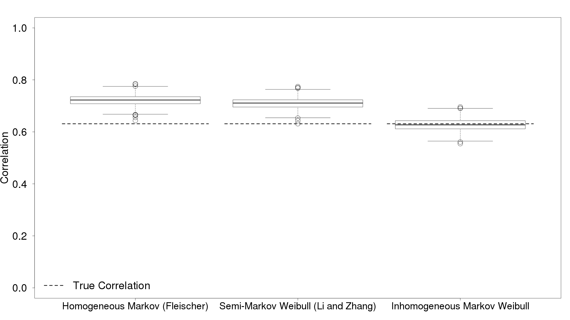
Figure 2: Estimated correlation coefficients for Weibull transition intensities (transition-specific shape parameter), time-inhomogeneous Markov process, $1000$ simulation runs. The horizontal line corresponds to the true correlation, received by plugging in the parametric assumption in the correlation formula in Section 2.5.

More results for alternative assumptions on the underlying transition hazards are provided in a web supplement.

6 Real data example

To illustrate the proposed methodology, we applied it to the data of CLEOPATRA⁴⁴, a large Phase 3 randomized clinical trial in HER2-positive metastatic breast cancer. In the trial, 808 patients were randomized. At the primary analysis with a clinical cutoff date of 13th May 2011, the key secondary endpoint investigator-assessed PFS (Inv-PFS) gave an estimated hazard ratio of 0.65 ([0.54, 0.78]). For OS, the hazard ratio was 0.64 ([0.47, 0.88]). After an additional interim analysis for OS with clinical cutoff date 14th May 2012, cross-over from the control to the treatment arm was allowed, and about 12% of the patients initially randomized to the control arm actually crossed over. Using a clinical cutoff of 11th February 2014 for the final analysis on OS, the estimated hazard ratios for Inv-PFS and OS were updated to 0.68 ([0.58, 0.80], based on 604 events) and 0.68 ([0.56, 0.84], 389 deaths), respectively ⁴⁵. In what follows, we analyze the data from this last snapshot.

As for the number of transitions, we observe 579 transitions $0\to 1$, 47 from $0\to 2$, and 342 from $1\to 2$.

6.1 Cumulative hazards

As a first illustration, in Figure 3 we provide estimates for the cumulative hazard functions for each transition, under various assumptions, and for all CLEOPATRA patients jointly. The two plots in the upper row and the left-most bottom row plots provide different estimates for the cumulative hazards for each transition in the IDM depicted in Figure 1: the entirely nonparametric Nelson-Aalen estimate, the two homogeneous Markov and semi-Markov parametric estimates assuming an exponential⁸ or Weibull⁹ model and our time-inhomogeneous Markov approach based on the counting process likelihood developed in this paper. For the $0\to 1$ transition all models provide a very similar and satisfactory fit. For the $0\to 2$ transition we find that the added flexibility of a model with two more shape parameters provides a better fit, as judged by visually comparing the parametric to the nonparametric estimate. As for the $1\to 2$ transition, we provide two graphs, accounting for the different time-scale of the various models. In the lower-left plot, the time-inhomogeneous Markov model seems to slightly overestimate the cumulative hazard of that transition, likely induced by the shape of the cumulative hazard function of the chosen Weibull distribution, which is an non-decreasing function through the origin. The estimates based on the homogeneous Markov and semi-Markov models by Fleischer et al. and Li and Zhang are depicted in the lower-right plot, with $x$-axis time scale time since progression.

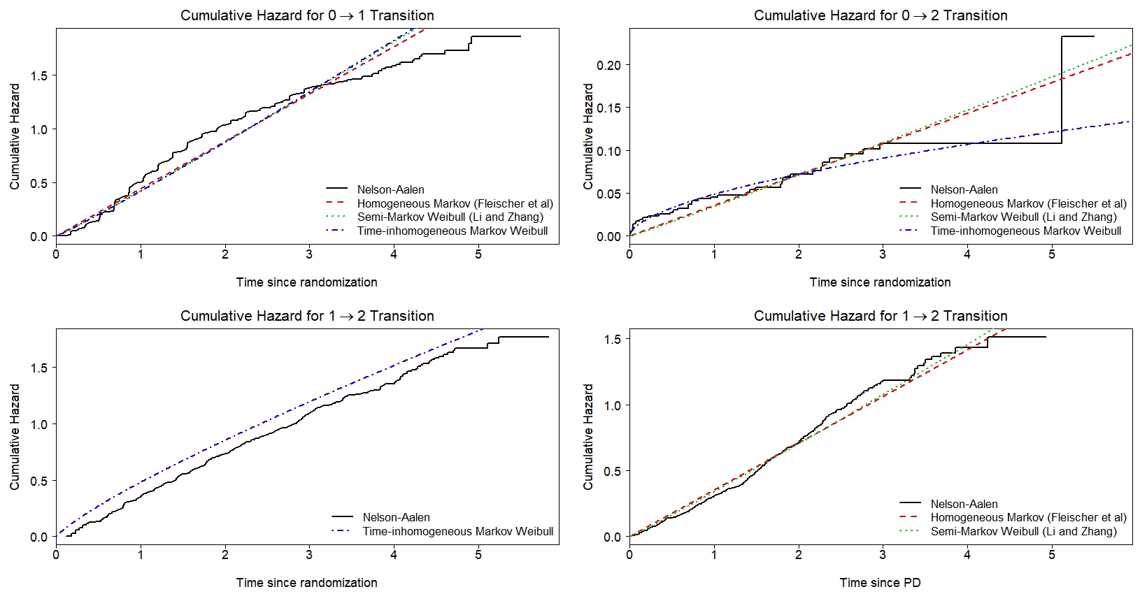
Figure 3: CLEOPATRA trial: estimates for cumulative hazards for each transition.

6.2 Survival functions

Figure 4 depicts estimates of survival functions for PFS and OS, based on plugging in estimates of cumulative hazards into the formulas for the transition probabilities and plugging these in in turn into the expressions for $S_{PFS}$ and $S_{OS}$. One of the questions that has been explored based on an IDM is to quantify the association between PFS and OS through estimation of Pearson’s correlation coefficient^{8, 9}. In order to see whether that association is different between control and treatment arm in CLEOPATRA, we split the plot by treatment arms. In general, judging goodness-of-fit of the parametric models through comparison with the nonparametric Kaplan-Meier estimate, we find that generally PFS is very similar for all the methods and in both treatment arms. This is not surprising, for the following reasons: first, the estimates of the cumulative hazard for the $0\rightarrow 1$ transition are very similar for the different methods. Second, the difference in estimates for the $0\rightarrow 2$ transition does not relevantly influence $S_{PFS}$ as the number of such transitions is relatively much lower compared to the number of $0\rightarrow 1$ transitions. Finally, since $S_{PFS}$ in (3) only depends on the hazards of the $0\to 1,2$ transitions it is agnostic to whether we assume a semi-Markov or Markovian model. Thus, similar estimates for $S_{PFS}$ are expected unless the estimated shape parameter of the Weibull model with restricted shape parameter⁹ for the $0\rightarrow 1$ transition differs relevantly from the one for our IM model.

The three methods also yield similar estimates for OS, which makes the differences seen in the goodness-of-fit in Figure 3 appear less important. One possible reason for this will be that $\mbox{PFS}=\mbox{OS}$ with positive probability.

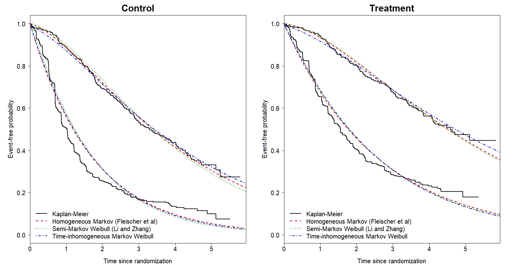
Figure 4: CLEOPATRA trial: various estimates of survival functions for OS (upper curves) and PFS (lower curves).

6.3 Inference for the correlation coefficient between PFS and OS

One important aspect when validating PFS as a potential surrogate endpoint for OS is to analyze their correlation ^{8, 9}. Fleischer et al. discuss that if the correlation is rather low it might not be reasonable to pursue a joint modelling of PFS and OS but to consider the two endpoints separately. According to the latter authors, even more important is the comparison of different correlation values for different substances, lines of treatment or indications. Examples for non-small cell lung cancer (NSCLC) ⁸ and prostate as well as larynx cancer ⁹ have been used to illustrate the methodology. Estimated correlations between PFS and OS range from 0.34 for a NSCLC example based on 95 patients in Fleischer et al. to 0.90 in an example based on 356 patients in Li and Zhang.

The estimated correlation coefficients for the CLEOPATRA trial in HER2-positive metastatic breast cancer are provided in Table 1. It is important to note that our proposed methods also allow to provide confidence intervals for these correlation coefficients. We find that irrespective of the method, the correlation between PFS and OS is lower in the control compared to the treatment arm. A potential reason for this is that after the primary analysis for PFS, crossover from the control to the treatment arm was allowed, potentially confounding the association between PFS and OS in the control arm. As for the various assumptions on $X$ and the parametric transition intensities, estimates for the correlation coefficient are rather comparable and likely not relevantly different taking into account estimation uncertainty. CLEOPATRA is quite a large trial, with 808 patients, 604 PFS and 389 OS events providing substantial information on PFS and OS. Still, confidence intervals around correlation coefficients have a width of up to 0.15 for the homogeneous Markov and the semi-Markov model (with the latter based on the same shape parameter for all transition intensities) and are even wider for the time-inhomogeneous Markov model with Weibull transition hazards. So, it seems precisely estimating the correlation coefficient is inherently a hard task even for this quite large dataset, and the precision crucially depends on the bias-variance trade-off taken, i.e. whether a more or less restrictive parametric model is entertained. Note that since neither for PFS nor OS the Kaplan-Meier estimate drop down to zero, we are not able to fully nonparametrically estimate the correlation coefficient.

On an absolute scale, the correlation coefficients estimated for CLEOPATRA under different model assumptions are comparable to those Li and Zhang⁹.

	Control arm	Treatment arm
Homogeneous Markov (Fleischer et. al)	0.543 [0.480; 0.609]	0.641 [0.571; 0.709]
Semi-Markov Weibull (Li and Zhang)	0.552 [0.489; 0.615]	0.644 [0.572; 0.718]
Time-inhomogeneous Markov Weibull	0.532 [0.434; 0.631]	0.567 [0.434; 0.680]

Table 1: CLEOPATRA trial: Estimated correlation coefficients between PFS and OS, including 95% confidence intervals based on 1000 bootstrap samples.

7 Discussion

We have suggested multistate modelling to jointly model occurrence of PFS and OS. The multistate framework improves on the commonly used latent times ^{20, 21, 8, 22, 23, 9, 24, 25} or copulas ^{5, 26, 27, 10, 28} in that it is the most parsimonious model. It works without hypothetical constructions while ensuring the natural properties that ${\rm PFS}\leq{\rm OS}$ and that equality holds with positive probability. We have demonstrated that the joint distribution of PFS and OS can be derived based on a multistate model. No further assumptions were required. The multistate model was allowed to be non-Markov, and we have only assumed that the model is sufficiently smooth in that the transition intensities exist. For illustration, we have demonstrated how to express the correlation between PFS and OS, which has received some attention recently ^{8, 9}. We have improved on these approaches by fitting them into our general framework and providing methods of statistical inference. The methods were then illustrated using data from a recent large randomized clinical trial.

The real data example also illustrated restrictions of using the correlation coefficient to quantify the dependence between PFS and OS. Firstly, and as is common in time-to-event outcomes, the Kaplan-Meier curves did not drop down to zero for PFS and OS. The implication is that not the entire distributions of PFS and OS can be identified nonparametrically, and this is in particular true for OS. As a consequence, parametric extrapolation would be required if one wanted to estimate the correlation coefficient based on these nonparametric estimates. Secondly, and almost irrespective of the goodness of the parametric fit, the main message from estimating the correlation was that the higher PFS, the higher OS. But this is, of course, no surprise, because ${\rm PFS}\leq{\rm OS}$.

Our approach allows for any parametric specification of the transition intensities, generalizing the use of constant hazards⁸ or Weibull⁹ hazards with common shape parameter. If goodness of fit is a concern, the transition probabilities of Section 2.4 can be estimated nonparametrically, either in a time-inhomogeneous Markov model ¹² or, provided that censoring is entirely random, even in a non-Markov model ⁴¹. However, this is only possible on the time interval of follow-up. If a (partially) nonparametrical analysis is desired, on would then need to parametrically model the remainder of the multistate distribution, again relying on extrapolation. An alternative would be to evaluate the integrals in Section 2.5 only up to the last observed event time, similar to the concept of restricted mean survival, but usefulness of such a restricted dependence measure would need to be further investigated. These issues call for further investigating how to adequately study the dependence between PFS and OS. We reiterate that whatever the choice of such a dependence measure may be, it would be a function of the joint distribution of PFS and OS and could hence be studied within our framework.

8 Acknowledgments

This paper summarizes and extends the results of the first author’s MSc thesis submitted at the University of Ulm. Part of the research for the thesis was conducted while the first author was still an intern in the Biostatistics Department of Hoffmann-La Roche in Basel. JB was partially supported by grant BE 4500/1-2 of the German Research Foundation (DFG).

Appendix A Closed formulas for transition probabilities and for $S_{PFS}$ and $S_{OS}$

In this section, we provide closed formulas for the transition probabilities $P_{ij}$ and survival functions for PFS and OS for $X(t)$ a semi-Markov, time-inhomogeneous Markov, and homogeneous Markov process. The non-Markov case requires further assumptions on how transition intensities depend on ${t_{1}}$, and we will not pursue this further here.

As discussed in Section 2, in the case of $X(t)$ being homogeneous Markov then the transition intensities are constant in time since origin (and independent of ${t_{1}}$) and thus exponential. Reversely put, if we assume “homogeneous” (i.e. $\alpha_{ij}$ independent of $t$ and ${t_{1}}$) exponentially distributed transition intensities, then the homogeneous and time-inhomogeneous Markov as well as the semi-Markov model all coincide. If we allow $\alpha_{12}$ to depend on ${t_{1}}$ then a more general non-Markov, or Markov extension in the terminology of Hougaard¹¹, assumption for $X(t)$ has to be entertained.

Fleischer et al. ⁸ (exponential) and Li and Zhang ⁹ (Weibull) assumed parametric models in a latent failure time model for the modelling of PFS and OS. As much as possible at all, we compare our results from a multistate model for $S_{PFS}$ and $S_{OS}$ to what they received.

Table 2 provides general formulas for transition probabilities under the various assumptions on $X(t)$.

	Non-Markov	Semi-Markov	Time-inhomogeneous	Homogeneous
			Markov	Markov (exponential)
$P_{00}$	$\exp\Bigl{(}-\int_{s}^{t}\alpha_{01}(u)+\alpha_{02}(u){\rm\;d}u\Bigr{)}$			$P_{00}^{\text{TH}}(s,t)$ below
$P_{11}$	$P_{11}^{\text{NM}}(s,t;{t_{1}}):=\exp\Bigl{(}-\int_{s}^{t}\alpha_{12}(u;t_{1}){\rm\;d}u\Bigr{)}$	$P_{11}^{\text{SM}}(s,t;{t_{1}}):=\exp\Bigl{(}-\int_{s}^{t}\alpha_{12}(u-t_{1}){\rm\;d}u\Bigr{)}$	$P_{11}^{\text{TI}}(s,t):=\exp\Bigl{(}-\int_{s}^{t}\alpha_{12}(u){\rm\;d}u\Bigr{)}$	$P_{11}^{\text{TH}}(s,t)$ below
$P_{22}$	1
$P_{01}$	$\int_{s}^{t}P_{00}(s,u_{-})\alpha_{01}(u)P_{11}^{\text{NM}}(u,t;u){\rm\;d}u$	$\int_{s}^{t}P_{00}(s,u_{-})\alpha_{01}(u)P_{11}^{\text{SM}}(u,t;u){\rm\;d}u$	$\int_{s}^{t}P_{00}(s,u_{-})\alpha_{01}(u)P_{11}^{\text{TI}}(u,t){\rm\;d}u$	$P_{01}^{\text{TH}}(s,t)$ below
$P_{12}$	$1-P_{11}^{\text{NM}}(s,t;{t_{1}})$	$1-P_{11}^{\text{SM}}(s,t;{t_{1}})$	$1-P_{11}^{\text{TI}}(s,t)$	$1-P_{11}^{\text{TH}}(s,t)$
$P_{02}$	combine (6) with the column-wise expressions for $P_{00}$ and $P_{11}$

Table 2: Formulas for transition probabilities $P_{lm}(s,t)$, for various assumptions on the process $X(t)$. See Appendix A.1 below for the homogeneous Markov case.

A.1 Exponential (time-constant) transition hazards

As for the homogeneous Markov or exponential case, we assume that the transition hazards in our multistate model in Figure 1 are constant and independent of ${t_{1}}$:

$$\alpha_{01}(t)\ =\ \lambda_{01},\hskip 28.45274pt\alpha_{02}(t)\ =\ \lambda_{02},\hskip 28.45274pt\alpha_{12}(t;{t_{1}})=\lambda_{12}.$$

Then, abbreviating $\lambda_{012}:=\lambda_{12}-\lambda_{01}-\lambda_{02}$,

$$P_{00}^{\text{TH}}(s,t) = \exp\Bigl{(}-\int_{s}^{t}\lambda_{01}+\lambda_{02}{\rm\;d}u\Bigr{)}\ =\ \exp\Bigl{(}-(\lambda_{01}+\lambda_{02})(t-s)\Bigr{)},$$

$$P_{11}^{\text{TH}}(s,t) = \exp\Bigl{(}-\int_{s}^{t}\lambda_{12}{\rm\;d}u\Bigr{)}\ =\ \exp\Bigl{(}-\lambda_{12}(t-s)\Bigr{)},$$

$$P_{01}^{\text{TH}}(s,t) = \int_{s}^{t}P_{00}^{\text{TH}}(s,u_{-})\lambda_{01}P_{11}^{\text{TH}}(u,t){\rm\;d}u\ =\ \lambda_{01}\int_{s}^{t}\exp\Bigl{(}-(\lambda_{01}+\lambda_{02})(u_{-}-s)\Bigr{)}\exp\Bigl{(}-\lambda_{12}(t-u)\Bigr{)}{\rm\;d}u$$

$$= \lambda_{01}\exp\Bigl{(}(\lambda_{01}+\lambda_{02})s-\lambda_{12}t\Bigr{)}\int_{s}^{t}\exp(\lambda_{012}u){\rm\;d}u$$

$$= \lambda_{01}\lambda_{012}^{-1}\Bigl{[}\exp\Bigl{(}-(\lambda_{01}+\lambda_{02})(t-s)\Bigr{)}-\exp\Bigl{(}-\lambda_{12}(t-s)\Bigr{)}\Bigr{]}.$$

We note that all these quantities depend on the interval limits $s$ and $t$ only through the difference $t-s$, as is expected for a time-homogeneous Markov model.

Plugging the expressions from Table 2 in (3) and (8) we get

$$S_{PFS}^{\text{TH}}(t) = P_{00}^{\text{TH}}(0,t)\ =\ \exp\Bigl{(}-(\lambda_{01}+\lambda_{02})t\Bigr{)}$$

and

$$S_{OS}^{\text{TH}}(t)\ =\ S_{PFS}^{\text{TH}}(t)+P_{01}^{\text{TH}}(0,t) = \frac{\lambda_{12}-\lambda_{02}}{\lambda_{012}}\exp\Bigl{(}-(\lambda_{01}+\lambda_{02})t\Bigr{)}+\frac{\lambda_{01}}{\lambda_{012}}\exp(-\alpha_{12}t).$$

Comparing $S_{PFS}^{\text{TH}}$ and $S_{OS}^{\text{TH}}$ to those in Theorem 5 in Fleischer et al.⁸ we find that these formulas are identical to those derived using the latent failure time assumption.

A.2 Weibull transition hazards

If a Weibull model should be entertained for the transition hazards, then we can either specify a time-inhomogeneous Markov or semi-Markov model as in Table 3.

	$\alpha_{01}$	$\alpha_{02}$	$\alpha_{12}$
time-inhomogeneous Markov	$\alpha_{01}(t)=\lambda_{01}\cdot\gamma_{01}t^{\gamma_{01}-1}$	$\alpha_{02}(t)=\lambda_{02}\cdot\gamma_{02}t^{\gamma_{02}-1}$	$\alpha_{12}(t)=\lambda_{12}\cdot\gamma_{12}t^{\gamma_{12}-1}$
semi-Markov			$\alpha_{12}(t;{t_{1}})=\lambda_{12}\cdot\gamma_{12}(t-{t_{1}})^{\gamma_{12}-1}$

Table 3: Weibull transition intensities.

Note that using the multistate formulation, Weibull intensities with transition-specific shape parameters can be used, no restriction to a common shape parameter as in Li and Zhang ⁹ is needed to be able to derive closed formulas.

For the time-inhomogeneous model, plugging in into (3) and (8) yields, after some straightforward algebraic manipulations,

$$S_{PFS}^{\text{TI}}(t)\ =\ P_{00}^{\text{SM}}(0,t) = \exp(-\lambda_{01}t^{\gamma_{01}}-\lambda_{02}t^{\gamma_{02}})$$

and

$$S_{OS}^{\text{TI}}(t) = S_{PFS}^{\text{TI}}(t)+P_{01}^{\text{TI}}(0,t)$$

$$= S_{PFS}^{\text{TI}}(t)+\lambda_{01}\gamma_{01}\int_{0}^{t}u^{\gamma_{01}-1}\cdot\exp\Bigl{(}-\lambda_{01}u^{\gamma_{01}}-\lambda_{02}u^{\gamma_{02}}-\lambda_{12}(t^{\gamma_{12}}-u^{\gamma_{12}})\Bigr{)}{\rm\;d}u$$

for the survival function for OS. As for the semi-Markov model, the hazard $\alpha_{12}=\alpha_{12}(t;{t_{1}})$ for the transition from PD to death not only depends on the actual time $t$, but also on the time ${t_{1}}$ of the transition out of the initial state. Similar manipulations yield $S_{PFS}^{\text{SM}}\ =\ S_{PFS}^{\text{TI}}$ for the survival function for PFS and

$$S_{OS}^{\text{SM}}(t) = S_{PFS}^{\text{SM}}(t)+P_{01}^{\text{SM}}(0,t)$$

$$= S_{PFS}^{\text{SM}}(t)+\lambda_{01}\gamma_{01}\int_{0}^{t}u^{\gamma_{01}-1}\cdot\exp\Bigl{(}-\lambda_{01}u^{\gamma_{01}}-\lambda_{02}u^{\gamma_{02}}-\lambda_{12}(t-u)^{\gamma_{12}}\Bigr{)}{\rm\;d}u$$

for the survival function for OS. Now, how do these expressions compare to those derived under a latent failure time assumption in Li and Zhang⁹ when setting $\gamma:=\gamma_{01}=\gamma_{02}=\gamma_{12}$? The survival function $S_{PFS}^{\text{TI}}=S_{PFS}^{\text{SM}}$ for PFS simplifies to that in the latter paper as does $S_{OS}^{\text{SM}}$. We would like to emphasize that the fact that the latent failure time and multistate model formulation lead to the same expressions for the semi-Markov case does not imply that the assumptions on $X(t)$ are identical for the latent failure time and the multistate model.

To conclude this section we note that (3) and (8) are general formulas based on the IDM. Closed formulas for other parametric models can easily be derived from these.

Appendix B Joint distribution of PFS and OS if $X$ is Markov

Equation (7) provides the expression of the joint distribution of PFS and OS for a general, not necessarily Markov, process $X$. If we assume $X$ to be Markov, then $P_{12}(u,v;{t_{1}})$ simplifies to $P_{12}(u,v)$ so that we can write (7) as

$$P({\rm PFS}\leq u,{\rm OS}\leq v) = 1-P_{00}(0,u)-P_{01}(0,u)P_{11}(u,v).$$

More specifically, if $X$ is homogeneous Markov we can plug in the formulas derived in Section A.1 to get

$$P({\rm PFS}\leq u,{\rm OS}\leq v) = 1-\lambda_{01}\lambda_{012}^{-1}\exp(-\lambda_{12}v)+\exp(-\lambda_{012}u)\Bigl{(}\lambda_{01}\lambda_{012}^{-1}\exp(-\lambda_{12}v)-\exp(-\lambda_{12}u)\Bigr{)}.$$

Corresponding formulas for alternative assumptions on $X$ can be derived analogously.

Appendix C Joint distribution of PFS and OS if $X$ is non-Markov

Here, we provide the general expression for the joint distribution of PFS and OS if $X$ is non-Markov. To this end, we need to evaluate $P(X(v)=2|X(u)=1)$ under that assumption. The following computations are repeatedly using the formula of total probability and conditioning. Assuming $u\leq v$ we have

$$P(X(v)=2|X(u)=1) = \int_{0}^{u}P(X(v)=2|X(u)=1,{\rm PFS}=t_{1}){\rm\;d}P({\rm PFS}\leq t_{1}|X(u)=1)$$ (10)

$$= \int_{0}^{u}P_{12}(u,v;t_{1}){\rm\;d}P({\rm PFS}\leq t_{1}|X(u)=1).$$

In 10, integration is w.r.t. $t_{1}$ and over the time interval $(0,u]$. Now, for $t_{1}\leq u$, we have that

$$P({\rm PFS}\leq t_{1}|X(u)=1) = P(X(t_{1})\in\{1,2\}|X(u)=1)$$

$$= P(X(t_{1})=1|X(u)=1)$$

$$= P(X(t_{1})=1,X(u)=1)/P(X(u)=1)$$

$$= P(X(t_{1})=1,X(u)=1)/P_{01}(0,u),$$ (12)

where (C) follows, because given the process is still in the intermediate state at $u$, $u\geq t_{1}$, $X(t_{1})=2$ is impossible. As for the nominator,

$$P(X(t_{1})=1,X(u)=1) = \int_{0}^{t_{1}}P(X(t_{1})=1,X(u)=1|{\rm PFS}=s){\rm\;d}P({\rm PFS}\leq s)$$

$$= \int_{0}^{t_{1}}P(X(u)=1|X(t_{1})=1,{\rm PFS}=s)P(X(t_{1})=1|{\rm PFS}=s){\rm\;d}P({\rm PFS}\leq s)$$

$$= \int_{0}^{t_{1}}P_{11}(t_{1},u;s)P(X(t_{1})=1|{\rm PFS}=s){\rm\;d}P({\rm PFS}\leq s)\ \ \ \text{by \eqref{eq:P11}.}$$

It remains to derive $P(X(t_{1})=1|{\rm PFS}=s)$ for $s\in(0,t_{1}]$. To this end,

$$P_{11}(s,t_{1};s) = P(X(t_{1})=1|X(s)=1,{\rm PFS}=s)$$

$$= P(X(t_{1})=1,X(s)=1|{\rm PFS}=s)/P(X(s)=1|{\rm PFS}=s)$$

$$= P(X(t_{1})=1|{\rm PFS}=s)/P(X(s)=1|{\rm PFS}=s)$$

because the event $\{X(s)=1\}$ is implied by the condition $\{{\rm PFS}=s\}$ together with noting that $X$ is still in state 1 at $t_{1}$, $t_{1}\geq s$. Now, the denominator in the last display is

$$P(X(s)=1|{\rm PFS}=s)=P(X({\rm PFS})=1|{\rm PFS}=s)=\frac{\alpha_{01}(s)}{\alpha_{01}(s)+\alpha_{02}(s)},$$

see our discussion on how to simulate PFS-OS trajectories in Section 2.1. Rearranging gives

$$P(X(t_{1})=1|{\rm PFS}=s) = \frac{\alpha_{01}(s)}{\alpha_{01}(s)+\alpha_{02}(s)}P_{11}(s,t_{1};s).$$

The last display has an interpretation: Conditional on PFS at time $s$ one is in the progression state at a later time $t_{1}$, if, firstly, one actually moves into the progression state at the time of PFS. Given a transition into the progression state at this time, secondly, one has to remain in the intermediate state of the model until time $t_{1}$. Putting everything together, we thus have

$$P({\rm PFS}\leq t_{1}|X(u)=1) = P_{01}(0,u)^{-1}\int_{0}^{t_{1}}P_{11}(t_{1},u;s)P_{11}(s,t_{1};s)\frac{\alpha_{01}(s)}{\alpha_{01}(s)+\alpha_{02}(s)}{\rm\;d}P({\rm PFS}\leq s).$$

Plugging this distribution function into (10) finally allows to compute $P(X(v)=2|X(u)=1)$ under a non-Markov assumption. We reiterate that our simulation approach in Section 2.1 may be a convenient alternative to evaluating these somewhat tedious formulas.

Appendix D Distribution function of ${\rm PFS}\cdot{\rm OS}$

We have that

$$P({\rm PFS}\cdot{\rm OS}>t) = P({\rm PFS}>\sqrt{t})+P({\rm PFS}\leq\sqrt{t},{\rm PFS}\cdot{\rm OS}>t).$$

When ${\rm PFS}\leq\sqrt{t},{\rm PFS}\cdot{\rm OS}>t$ is only possible, if $X({\rm PFS})=1$. Hence, we can express the last probability as

$$P({\rm PFS}\leq\sqrt{t},{\rm PFS}\cdot{\rm OS}>t) = \int P({\rm PFS}\leq\sqrt{t},{\rm PFS}\cdot{\rm OS}>t\,|\,{\rm PFS}=u,X({\rm PFS})=1)\,{\rm\;d}P({\rm PFS}\leq u,X({\rm PFS})=1)$$

$$= \int_{(0,\sqrt{t}]}P({\rm OS}>t/u\,|\,{\rm PFS}=u,X({\rm PFS})=1)\,{\rm\;d}P({\rm PFS}\leq u,X({\rm PFS})=1)$$

$$= \int_{(0,\sqrt{t}]}P_{11}(u,t/u;u)\,{\rm\;d}P({\rm PFS}\leq u,X({\rm PFS})=1).$$

It remains to compute $P({\rm PFS}\leq u,X({\rm PFS})=1)$, but this is nothing else than the cumulative incidence function of a competing risk, i.e. the expected proportion of individuals experiencing progression over the course of time. It can be computed according to

$$P({\rm PFS}\leq u,X({\rm PFS})=1) = \int_{0}^{u}P({\rm PFS}>s-)\alpha_{0{\color[rgb]{0,0,1}1}}(s){\rm\;d}s$$

$$= \int_{0}^{u}S_{PFS}(s-)\alpha_{0{\color[rgb]{0,0,1}1}}(s){\rm\;d}s,$$

see e.g. Equation (3.11) in Beyersmann et al.¹⁵.

References

- 1 U.S. Food and Drug Administration . Guidance for Industry: Clinical Trial Endpoints for the Approval of Cancer Drugs and Biologics.2007.
- 2 Pazdur R.. Endpoints for assessing drug activity in clinical trials. Oncologist. 2008;13 Suppl 2:19–21.
- 3 George S. L., Wang X., Pang H.. Cancer Clinical Trials: Current and Controversial Issues in Design and Analysis. CRC Biostatistics SeriesChapman & Hall; 2016.
- 4 Saad E. D., Buyse M.. Statistical controversies in clinical research: end points other than overall survival are vital for regulatory approval of anticancer agents. Ann. Oncol.. 2016;27(3):373–378.
- 5 Burzykowski Tomasz, Molenberghs Geert, Buyse Marc, Geys Helena, Renard Didier. Validation of surrogate end points in multiple randomized clinical trials with failure time end points. Journal of the Royal Statistical Society: Series C (Applied Statistics). 2001;50(4):405–422.
- 6 Buyse M., Molenberghs G., Paoletti X., et al. Statistical evaluation of surrogate endpoints with examples from cancer clinical trials. Biom J. 2016;58(1):104–132.
- 7 V Prasad, C Kim, M Burotto, A Vandross. The strength of association between surrogate end points and survival in oncology: A systematic review of trial-level meta-analyses. JAMA Internal Medicine. 2015;175(8):1389–1398.
- 8 Fleischer Frank, Gaschler-Markefski Birgit, Bluhmki Erich. A statistical model for the dependence between progression-free survival and overall survival. Statistics in Medicine. 2009;28(21):2669–2686.
- 9 Li Yimei, Zhang Qiang. A Weibull multi-state model for the dependence of progression-free survival and overall survival. Statistics in Medicine. 2015;34(17):2497–2513.
- 10 Fu H., Wang Y., Liu J., Kulkarni P. M., Melemed A. S.. Joint modeling of progression-free survival and overall survival by a Bayesian normal induced copula estimation model. Stat Med. 2013;32(2):240–254.
- 11 Hougaard P.. Analysis of Multivariate Survival Data. Statistics for Biology and HealthSpringer New York; 2000.
- 12 Aalen Odd, Borgan Ornulf, Gjessing Haakon. Survival and event history analysis: a process point of view. Springer Science & Business Media; 2008.
- 13 Weber Enya M., Titman Andrew C.. Quantifying the association between progression-free survival and overall survival in oncology trials using Kendall’s . Statistics in Medicine. ;0(0).
- 14 Andersen PK, Keiding N. Multi-state models for event history analysis. Statistical Methods in Medical Research. 2002;11(2):91–115.
- 15 Beyersmann Jan, Allignol Arthur, Schumacher Martin. Competing Risks and Multistate Models with R. Springer, New York; 2012.
- 16 Beyersmann J, Latouche A, Buchholz A, Schumacher M. Simulating competing risks data in survival analysis.. Statistics in Medicine. 2009;28:956–971.
- 17 Putter H., Fiocco M., Geskus R. B.. Tutorial in biostatistics: competing risks and multi-state models. Stat Med. 2007;26(11):2389–2430.
- 18 Andersen P. K., Pohar Perme M.. Inference for outcome probabilities in multi-state models. Lifetime Data Anal. 2008;14(4):405–431.
- 19 Andersen Per Kragh. Life years lost among patients with a given disease. Statistics in Medicine. 2017;36(22):3573–3582.
- 20 Buyse M., Piedbois P.. On the relationship between response to treatment and survival time. Statistics in Medicine. 1996;15:2797–2812.
- 21 Goldman B., LeBlanc M., Crowley J.. Interim futility analysis with intermediate endpoints. Clin Trials. 2008;5(1):14–22.
- 22 Heng D. Y., Xie W., Bjarnason G. A., et al. Progression-free survival as a predictor of overall survival in metastatic renal cell carcinoma treated with contemporary targeted therapy. Cancer. 2011;117(12):2637–2642.
- 23 Crowther Michael J, Lambert Paul C. Simulating biologically plausible complex survival data. Statistics in Medicine. 2013;32(23):4118–4134.
- 24 Xia F., George S. L., Wang X.. A Multi-state Model for Designing Clinical Trials for Testing Overall Survival Allowing for Crossover after Progression. Stat Biopharm Res. 2016;8(1):12–21.
- 25 Nomura S., Hirakawa A., Hamada C.. Sample size determination for the current strategy in oncology phase 3 trials that tests progression-free survival and overall survival in a two-stage design framework. J Biopharm Stat. 2017;.
- 26 Weir Christopher J, Walley Rosalind J. Statistical evaluation of biomarkers as surrogate endpoints: a literature review. Statistics in medicine. 2006;25(2):183–203.
- 27 Buyse Marc, Burzykowski Tomasz, Carroll Kevin, et al. Progression-free survival is a surrogate for survival in advanced colorectal cancer. Journal of clinical oncology. 2007;25(33):5218–5224.
- 28 Emura T., Nakatochi M., Murotani K., Rondeau V.. A joint frailty-copula model between tumour progression and death for meta-analysis. Stat Methods Med Res. 2017;26(6):2649–2666.
- 29 Kalbfleisch J., Prentice Ross. The Statistical Analysis of Failure Time Data. 2nd Ed. Wiley, Hoboken; 2002.
- 30 Aalen Odd. Dynamic modelling and causality. Scandinavian Actuarial Journal. 1987;:177–190.
- 31 Chiang Chin Long. Competing risks in mortality analysis. Annual review of public health. 1991;12(1):281–307.
- 32 Fan J., Prentice R. L., Hsu L.. A class of weighted dependence measures for bivariate failure time data. Journal of the Royal Statistical Society: Series B (Statistical Methodology). 2000;62(1):181–190.
- 33 Andersen Per Kragh, Borgan Ornulf, Gill Richard D., Keiding Niels. Statistical Models Based on Counting Processes. Springer; 1993.
- 34 Cube M., Schumacher M., Wolkewitz M.. Basic parametric analysis for a multi-state model in hospital epidemiology. BMC Med Res Methodol. 2017;17(1):111.
- 35 Efron B.. Censored Data and the Bootstrap. J. Amer. Statist. Assoc.. 1981;76:312–319.
- 36 Bluhmki Tobias, Schmoor Claudia, Dobler Dennis, et al. A wild bootstrap approach for the Aalen-Johansen estimator. Biometrics. ;0(0).
- 37 Gill Richard D., Wellner Jon A., Praestgaard Jens. Non- and Semi-Parametric Maximum Likelihood Estimators and the Von Mises Method (Part 1) [with Discussion and Reply]. Scandinavian Journal of Statistics. 1989;16(2):97-128.
- 38 Datta Somnath, Satten Glen A.. Validity of the Aalen-Johansen estimators of stage occupation probabilities and Nelson-Aalen estimators of integrated transition hazards for non-Markov models. Statistics and Probability Letters. 2001;55(4):403–411.
- 39 Aalen Odd. Nonparametric inference for a family of counting processes. The Annals of Statistics. 1978;:701–726.
- 40 Aalen Odd O, Johansen Søren. An empirical transition matrix for non-homogeneous Markov chains based on censored observations. Scandinavian Journal of Statistics. 1978;:141–150.
- 41 Putter H., Spitoni C.. Non-parametric estimation of transition probabilities in non-Markov multi-state models: The landmark Aalen-Johansen estimator. Stat Methods Med Res. 2018;27(7):2081–2092.
- 42 Meira-Machado Luís, Uña-Álvarez Jacobo, Cadarso-Suárez Carmen. Nonparametric estimation of transition probabilities in a non-Markov illness–death model. Lifetime Data Analysis. 2006;12(3):325–344.
- 43 Zeng Leilei, Cook Richard J., Lee Ker-Ai. Design of cancer trials based on progression-free survival with intermittent assessment. Statistics in Medicine. ;37(12):1947-1959.
- 44 Baselga J., Cortes J., Kim S. B., et al. Pertuzumab plus trastuzumab plus docetaxel for metastatic breast cancer. N. Engl. J. Med.. 2012;366(2):109–119.
- 45 Swain S. M., Baselga J., Kim S. B., et al. Pertuzumab, trastuzumab, and docetaxel in HER2-positive metastatic breast cancer. N. Engl. J. Med.. 2015;372(8):724–734.