STAIRoute: Early Global Routing using Monotone Staircases for Congestion Reduction

Abstract

With aggressively shrinking process nodes, physical design methods face severe challenges due to poor convergence and uncertainty in getting an optimal solution. An early detection of potential failures is thus mandated. This has encouraged to devise a feedback mechanism from a lower abstraction level of the design flow to the higher ones, such as placement driven synthesis, routability (timing) driven placement etc.

Motivated by this, we propose an early global routing framework using pattern routing following the floorplanning stage. We assess feasibility of a floorplan topology of a given design by estimating routability, routed wirelength and vias count while addressing the global congestion scenario across the layout. Different capacity profiles for the routing regions, such as uniform or non-uniform different cases of metal pitch variation across the metals layers ensures adaptability to technology scaling. The proposed algorithm STAIRoute takes $O(n^{2}kt)$ time for a given design with $n$ blocks and $k$ nets having at most $t$ terminals. Experimental results on a set of floorplanning benchmark circuits show $100\%$ routing completion, with no over-congestion in the routing regions reported. The wirelength for the $t$-terminal ($t\geq$ 2) nets is comparable with the Steiner length computed by FLUTE. An estimation on the number of vias for different capacity profiles is also presented, along with congestion and runtime results.

1 Introduction

In IC design flow, global routing (GR) is indispensable, particularly as an aide to detailed routing (DR) of the wires through different metal layers. Shrinking feature dimensions with technological advances in IC fabrication process pose more challenges on the physical design phase. There has been a tremendous increase in routing constraints arising from not only stringent layout design rules but also process variations and sub-wavelength effects of optical lithography. Successful routing completion of the nets without too many iterations or sacrifice in the performance of the designs is thus mandated.

Figure 1: Physical Design Flow: (a) Conventional, and (b) Proposed

In traditional grid graph based post-placement routing methods, multi-terminal nets are decomposed into two terminal segments using Steiner tree decomposition using Rectilinear minimum spanning tree (RMST) royj , or Rectilinear Steiner minimal tree (RSMT) panm1 topology as an initial solution with minimum length. Subsequently, congestion driven routing for each two terminal net segment is adopted through the routing regions. The congestion models in those methods have been formulated based on the capacity of the grids and the routing demands through them, along with a penalty function. For any unsuccessful routing due to over congestion ($\geq 100\%$), Rip-up and Re-reroute (RRR) techniques using maze routing lee ; sherw have been applied for possible routing completion while compromising in routed wirelength due to detour. The major challenge in the event of unsuccessful routing is to get back to placement stage in order to generate a new placement solution, but with no guarantee for successful routing completion (vide Figure 1 (a)). This may lead to several iterations until the goal is achieved and thus prove to be very costly if the entire design implementation is not completed within a stipulated time frame. In other words, this may have severe impact on time-to-market of the intended design.

The possibility of recurring iterations at the placement stage (vide Figure 1 (a)) due to failure at global routing stage may however be avoided if we can predict the feasibility of global routing as early as at the floorplanning stage, as depicted in Figure 1 (b). This comprises of the identification of monotone staircase regions as routing resources while estimating their capacity and formulating the congestion model. These types of routing resources are known to have advantages of acyclic routing order for successful routing completion ssk ; guru and avoidance of switch box routing sherw . They also allow easy channel resizability guru to mitigate heavy congestion ($\geq 100\%$).

Pattern routing such as single bend (L shaped) kast , two bend (Z shaped) kast ; panm1 , or even with more bends such as monotone staircase patterns zcao ; ychang ; luj in global routing has increased significantly in order to find a suitable routing path for a given net. In the recent past, single bend (L shaped) kast , two bend (Z shaped) kast ; panm1 , or even with more bends such as monotone staircase patterns zcao ; ychang has gained significant importance in grid-based global routing. With the increasing number of bends, these patterns yield more flexibility in order to find a possible routing path, but at the cost of more vias, if feasible. It was also shown that pattern based routing kast is much faster than maze routing, while monotone staircase pattern routing zcao has the same time complexity as with Z shaped patterns. A thoughtful trade off between routability (also wirelength) and the number of vias has to be made while keeping in mind that the routing resources are not over congested. Recent work on monotone staircase bipartitioning method karb3 attempted to address the minimization of the number of vias along a monotone staircase routing path by minimizing the number of bends in it zcao . Additionally, the pattern based routing are shown to help in cross talk minimization kast .

1.1 Outline of this work

In this paper, we present a new paradign in routability assessment following the floorplanning stage. The proposed routing model uses monotone staircase regions identified in a given floorplan for assessing routing completion without allowing any over-congestion in any of these routing regions. It is important to note that this routing model is different than the grid graph based model used in the post-placement global routers zcao ; kast ; mcho1 ; panm1 ; royj ; ychang ; kdai ; wliu . The outline of the proposed early global routing method, we call it STAIRoute, presented in Figure 2 as follows:

1. Identification of routing regions in a given floorplan by using a monotone staircase bipartitioning algorithm such as karb ; karb3 ;

2. Graph theoretic formulation based on these regions is used to determine a feasible routing paths for the given nets; uses congestion aware layer-assignment approach.

3. Routing order of the nets based on half perimeter wire length (HPWL) and the number of terminals (Netdegree);

4. Multi-terminal net decomposition to identify a set of two-terminal net segments using minimum spanning tree algorithm; obtained a new Steiner tree topology;

5. Routing through a number of metal layers using a shortest path algorithm to find an acceptable routing path;

6. Ensuring congestion in the routing regions is restricted to $100\%$ across the metal layers;

7. Supporting both unreserved and reserved layer based routing; provides an estimation on the number of vias for possible layer change along the routing paths.

Figure 2: Outline of the proposed early global routing framework

This paper is organized as follows: Section 2 revisits the preliminaries of monotone staircase bipartitioning method followed by Section 3 that includes related topics and the proposed global routing method using monotone staircases as the routing resources. Results are presented in Sections 4, and the concluding remarks in 5.

2 Preliminaries on Monotone Staircase Regions

In this section, we review the monotone staircase regions in a given floorplan and the floorplan birpartitioning framework to obtain them. Methods for top-down hierarchical monotone staircase bipartitioning of floorplans, both in Area-balanced and Number-balanced bipartition appear in dasg ; karb ; karb3 ; majum1 ; majum2 . Area-balanced bipartition is employed when the area of the blocks in a given floorplan have significant variance whereas Number-balanced bipartition is applicable for negligible variance in the area of the blocks. In majum1 ; majum2 , the balanced bipartitioner used iterative max-flow based yang min-cut algorithm and thereby incurred higher time complexity at each level of the hierarchy. In dasg , emphasis has been given merely to the hierarchical number balanced monotone staircase bipartitioning using depth-first traversal method in linear time at a given level of the hierarchy.

Figure 3: A floorplan with staircase regions and the corresponding ms-cuts in its block adjacency graph (BAG): (a) monotone increasing staircase (MIS), (b) monotone decreasing staircase (MDS) karb

Recently, a faster yet more accurate top-down hierarchical monotone staircase bipartition karb has been proposed to generate monotone staircase cuts, abbreviated as ms-cut as we subsequently refer to it. This algorithm takes $O(nk\log n)$ time and also ensures ms-cuts of increasing (decreasing) orientation at alternate levels of the hierarchy (vide Figure 4 (a) and (b)), namely MSC tree.

In order to identify monotone increasing (decreasing) staircase regions ($C_{I}$ ($C_{D}$) as depicted in Figure 3 (a) ((b)), abbreviated as MIS (MDS), for a given a planar embedding of a floorplan topology with $n$ blocks, an unweighted directed graph karb ; majum1 , called block adjacency graph (BAG) $G(V_{b},E_{b})$ is formulated. The graph is defined as follows: $V_{b}$ = $\{b_{i}|\forall$ blocks $b_{i}$ in the floorplan$\}$ and $E_{b}=\{<b_{i},b_{j}>|$ block $b_{i}$ is either on the left of or above (below) its adjacent block $b_{j}\}$. Note that $|V_{b}|$ = $n$ and $|E_{b}|$ = $3(n-1)$ (vide Lemma 2).

Lemma 1.

Given a floorplan with $n$ blocks, its MSC tree $(V_{m},E_{m})$ corresponding to the set $C$ of monotone staircase regions has $n-1$ ms-cuts (internal nodes).

Proof.

In a full binary tree, an internal node has two children (out degree = $2$) whereas an external (leaf) node has no children (out degree = 0). In our case, the internal nodes correspond to the ms-cuts in the MSC tree, and the external nodes are the blocks in the given floorplan.
Hence $\sum_{i}$OutDeg($v_{i}$) = $|E_{m}|$ = $|V_{m}|-1$, where $T_{m}$ = $G(V_{m},E_{m})$ is the resulting MSC tree as shown in Figure 4(b).
$\Rightarrow$ $2*|C|$ + $0*n$ = ($|C|$ + $n$) -1; where $|C|$ and $n$ are the number of ms-cuts and blocks respectively.
$\Rightarrow$ $|C|$ = $n-1$.
∎

3 This Work

The contribution in this paper is to propose a new routing model based on the floorplan bipartitioning results for a given design. Then we showcase how this routing model is used to estimate several routability metrices such as routing completion, routed wirelength, via count and the global congestion scenario, for a given number of metal layers. Following sections discuss about this work in detail.

3.1 Routing Region Definition

Using the recent hierarchical monotone staircase bipartition framework karb , we obtain a set of MIS (MDS) regions $C$ = {$C_{i}$} at alternate levels of the hierarchy in MSC tree. For the rest of the paper, we refer region and segment to monotone staircase region and its rectilinear segment respectively. These regions are used as the routing resources for the proposed early global routing framework.

Each region consists of one or more rectilinear segments, bounded by a distinct pair of blocks. For each segment in a region, the number of nets to be routed through it is estimated from the number of cut nets in the respective ms-cut node in the MSC tree. This is denoted as reference capacity $r_{k}$ for the $k$th segment. At any point during routing, its capacity usage $u_{k}$ (also known as routing demand in the existing literature), gives the region utilization.

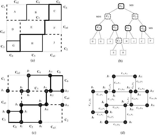
Figure 4: A floorplan along with: (a) its hierarchy of monotone staircase regions, (b) the corresponding MSC tree, (c) T-junctions at which staircases intersect, and (d) the corresponding junction graph

As in Figure 3 (a), the highlighted ms-cut $C_{I}$ on BAG contains seven cut edges {$GH$, $DH$, $EH$, $EJ$, $EF$, $BF$ and $BC$} corresponds to an MIS region $C_{I}$ having seven segments. Additionally, it has two more horizontal segments: one for the bottom side of the block $G$ at the bottom-left corner with the boundary of the floorplan while the other is on the top side of the block $C$ at the top-right corner of the floorplan. Likewise, an MDS region $C_{D}$ having six segments is illustrated in Figure 3 (b). Overall, a flooplan along with a set of MIS/MDS regions $C_{0}$ to $C_{7}$ is shown in Figure 4 (a). Regions with one segment having either vertical or horizontal orientation are termed as degenerated staircase regions, $C_{7}$ being such an example of such a degenerated region.

However, there exist a few more isolated segments along the boundary of the floorplan that are not identified as part of the MSC tree generation, and can be termed as non-MS regions. In Figure 4(a), $C_{n1}$ to $C_{n4}$ are the examples of few such regions. Their routing capacity $r_{k}$ is computed based on the number terminals on it, and those with nonzero $r_{k}$ contribute to routing as valid routing resources.

3.2 Routing Model: the Junction Graph (JG)

Now, we present our routing model using a set of monotone staircase regions and their intersection points, called T-junctions (vide Figure 4 (c)). It is evident that there exists a segment between each pair of adjacent T-junctions, henceforth referred as $junctions$.

Lemma 2.

Given a floorplan with $n$ blocks, the number of T junctions in it is $2n-2$.

Proof.

Every internal face in BAG corresponds to a T-junction, and is bounded by $3$ edges. Thus we have $3(f-1)$ = $2m$ excluding the exterior face, where $f$ and $m$ being the number of faces and edges in BAG respectively. Using Euler formula of $n-m+f=2$ for planar graphs, and replacing $f$ by $2m/3+1$, we get $m=3(n-1)$.
Hence, the number of T-junctions in the floorplan = $f-1$ = $2m/3$ = $2n-2$. ∎

Using the notion of T-junctions, we construct a weighted undirected graph (vide Figure 4(d)), called junction graph, $G_{j}$ = ($V_{j}$,$E_{j}$), where $V_{j}$ = $\{J_{p}\}$ corresponds to a set of junctions, and $E_{j}$ = {{$J_{p}$,$J_{q}$} $|$ as a pair of adjacent junctions $\{J_{p},J_{q}\}$ with a segment $s_{k}$ of a region $C_{m}\in C$ between them}. As depicted in Figure 4 (c), all the junctions, except those near the corners of the floorplan with degree two, have degree of three in $G_{j}$, i.e., have edges with three adjacent junctions. Using Lemma 2, it can be shown that $|E_{j}|$ = $3n-7$.

The weight of each edge $e_{pq}\in E_{j}$ is computed as:

$$wt(e_{pq})=length_{(}s_{k})/(1-p_{k})$$ (1)

where $p_{k}$, the normalized usage through the segment $s_{k}$, is defined as:

$$p_{k}=u_{k}/r_{k}$$ (2)

And, we define $(1-p_{k})$ as the usage penalty on the edge weight for routing a net through the corresponding segment $s_{k}$. In Figure 5, we illustrate the variation of edge weight with respect to the normalized usage $p_{k}$.

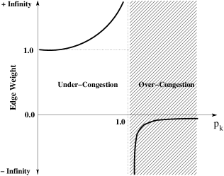
Figure 5: Edge weight ($wt(e_{pq})$) vs. normalized usage ($p_{k}$)

In the proposed routing framework, congestion is avoided in all the segments by restricting $p_{k}$ to be no more than $1.0$. This is achieved by setting the edge weight to Infinity whenever $p_{k}=1.0$. The corresponding edge is virtually removed from $E_{j}$. This ensures that the case of $p_{k}>1.0$ does not occur. In Figure 5, we mark the regions $p_{k}\leq 1.0$ and $p_{k}>1.0$ as Under-Congestion and Over-Congestion regions respectively. Therefore, we restrict to Under-Congestion while formulating the global routing graph such that there is no congestion in any of the routing resources. However, it may be noted that routing may fail for some of the nets due to insufficient capacity of some of the routing resources for a specified number of metal layers.

Lemma 3.

The construction of the junction graph takes $O(n)$ time.

Proof.

By Lemma 2, we know that there are $O(n)$ edges in the BAG, where each edge corresponds to a segment. Therefore, for each segment $s_{k}$ having a pair of junctions {$J_{p}$,$J_{q}$} as its endpoints, an edge is inserted in the $G_{j}$. Hence, the construction of the junction graph $G_{j}$ takes $O(n)$ time. ∎

3.2.1 Routing Model: the Global Staircase Routing Graph (GSRG)

In this section, we present our proposed global routing framework by extending the junction graph $G_{j}$ for each net.

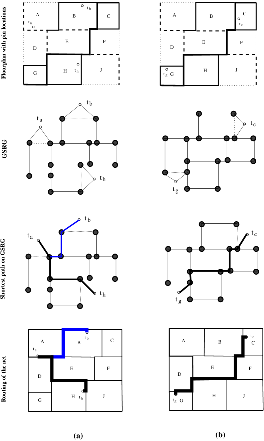
Figure 6: Steps for constructing the Global staircase routing graph (GSRG) from the Junction graph for (a) a $3$-terminal net $n_{i}=\{t_{a},t_{b},t_{h}\}$, and (b) a $2$-terminal net $n_{j}=\{t_{c},t_{g}\}$, along with corresponding routed paths in GSRG and finally routed nets in the floorplan topology

Let $N$ be a set of nets for a given floorplan. For each $t$-terminal ($t\geq 2$) net $n_{i}\in N$, we use $G_{j}$ as the backbone to derive the corresponding Global Staircase Routing Graph (GSRG) as depicted in Figure 6 (a) and 6 (b). The GSRG is defined as $G_{r}^{i}$ = ($V_{r}^{i}$,$E_{r}^{i}$), where $V_{r}^{i}$ = $V_{j}$ $\bigcup$ {$t_{l}|t_{l}\in n_{i}$}, and $E_{r}^{i}$ = $E_{j}\bigcup E_{lp}$. Each pin-junction edge $e_{lp}\in E_{lp}$ is defined as $e_{lp}$ = {$t_{l}$,$J_{p}$} $|$ $\forall t_{l}\in n_{i}$ and $\exists J_{p}\in J$, the pin $t_{l}$ resides on a segment $s_{k}$ associated with the junction $J_{p}$}. As before, we calculate the weight of a pin-junction edge $e_{lp}$ as:

$$wt(e_{lp})=\mathrm{distance}(t_{l},J_{p})/(1-p_{k}).$$ (3)

and define $(1-p_{k})$ as the usage penalty on the edge weight for routing a net through the corresponding segment $s_{k}$.

Lemma 4.

For a $t$-terminal net, the construction of its GSRG takes $O(t)$ time.

Proof.

As defined, the GSRG $G_{r}^{i}$ = ($V_{r}^{i}$,$E_{r}^{i}$) for a given net $n_{i}$ with $t$ terminals is obtained by augmenting the junction graph $G_{j}$ = ($V_{j},E_{j}$). In other words, $V_{j}$ is extended by $t$ terminals connected to $n_{i}$ in order to obtain $V_{r}^{i}$. It is also to be noted that each terminal resides on a segment $s_{k}$, having a pair of junctions ($J_{p},J_{q}$) on either ends. Therefore, each terminal (pin) contributes $2$ pin-junction edges and thus total $2t$ edges to $G_{r}^{i}$ for all $t$ terminals. Hence, the construction of $G_{r}^{i}$ takes $O(t)$ time for each net. ∎

After routing a net $n_{i}$ successfully, we update $u_{k}$ for all such segments $s_{k}$ through which $n_{i}$ is routed. Subsequently, the weights of the edges in $G_{j}$ are updated before we route the subsequent net $n_{i+1}$. When congestion is about to occur in a given segment ($p_{k}=1$), the weight of the corresponding edge in $G_{r}^{i}$ becomes Infinity. No routing is possible through such segments and the relevant edges virtually disappear making $G_{r}^{i}$ more sparse after each iteration of routing. To summarize, the normalized usage $p_{k}$ in this framework is constrained to a maximum of $100\%$, thus restricting the number of routed nets ($u_{k}$) through a given segment to be no more than its capacity ($r_{k}$).

In order to extend this model for $M(\geq 1)$ metal layers, we keep a parameter called currLayer($s_{k}$) associated with each segment $s_{k}$, initialized to $1$ and can go up to a maximum of $M$ metal layers. When congestion is about to occur in $s_{k}$ ($p_{k}=1$), we increment currLayer($s_{k}$) to the subsequent metal layer. Here the subsequent metal layer has different implication in (un)reserved layer model; the subsequent layer can either be one layer above currLayer($s_{k}$) or the next permitted layer based on the particular (horizontal/vertical) orientation of $s_{k}$ in the corresponding reserved layer model. This means that the resource $s_{k}$ has exhausted its entire capacity (i.e. $u_{K}=r_{k}$) for the current metal layer and is now ready for routing the nets through it for the next metal layer restricted by $M$. In this regard, the variation of $r_{k}$ across the metal layers (up to $M$) plays a significant role and thus directly impacts the routing completion of all the nets.

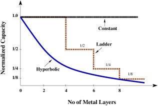
(a)

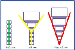
(b)

Figure 7: (a) Normalized Capacity profile of a routing resource ($s_{k}$) vs number of metal layers ($M$), and (b) Metal layer variation across process nodes m_pitch

In Figure 7 (a), we study different scenario of uniform as well as varying capacity profile for all the routing resources $s_{k}$ across the metal layers. In case of Uniform profile, $r_{k}$ carries the same value across the metal layers. We consider two different varying capacity profiles, one is Hyperbolic ($1/M$) type pattern, while the other being a Ladder type pattern. In case of the former, $r_{k}$ is more aggressively scaled across the metal layers, the latter is a more realistic scenario that captures the latest trend of the metal pitch/width variation across the metal layers in the recent nanometer technologies (vide Figure 7 (b) m_pitch ).

3.3 Multi-terminal Nets and Their Two-terminal Decomposition

In a global routing framework, routing a $t(>2)$-terminal net is crucial and obtaining an efficient solution for minimal length is a hard problem. Several works have been done so far to obtain the best possible $t-1$ net segments for a $t$-terminal net such as Rectilinear Steiner Minimal Tree (RSMT) topology proposed in FLUTE cchu based on a well defined grid structure known as Hanan grid hana ; sherw . Since the proposed work is based on a gridless framework and the routing regions are aligned with the MIS/MDS regions, we cannot adopt any grid-based RSMT framework such as FLUTE cchu .

Therefore, we propose a new method for multi-terminal net decomposition suitable for the proposed global routing framework. We construct a complete undirected graph for a given $t$-terminal ($t>2$) net $n_{i}\in N$, $G_{c}^{i}$ = ($V_{c}^{i}$,$E_{c}^{i}$) such that $V_{c}^{i}$ = {$t_{k}$}, $\forall t_{k}\in n_{i}$ and $E_{c}^{i}$ = {{$t_{j}$,$t_{k}$} $|$ $\forall t_{j},t_{k}\in n_{i}$ and $t_{j}\neq t_{k}$}. The weight of each edge $e_{jk}$ = {$t_{j}$,$t_{k}$} $\in E_{c}^{i}$ is computed as half the perimeter length (HPWL) of the bounding box for each terminal pair ($t_{i},t_{j}$) (vide Figure 8 (a)). It is evident that $|V_{c}^{i}|$ = $O(t)$ and $|E_{c}^{i}|$ = $O(t^{2})$. By employing $O(n^{2})$ Prim’s Minimum Spanning Tree (MST) algorithm cormen , we obtain a minimum spanning tree (MST) $T^{i}$ for $G_{c}^{i}$ having $t-1$ edges, i.e., $t-1$ valid $2$-terminal pairs. For each edge $e_{jk}$ = {$t_{j}$, $t_{k}$} $\in T^{i}$, we perform 2-terminal net routing by applying Dijkstra’s single source shortest path algorithm cormen . Once we obtain the routing for all such terminal pairs, we obtain the Steiner points by identifying the common routing segments as illustrated by an example in Figure 8.

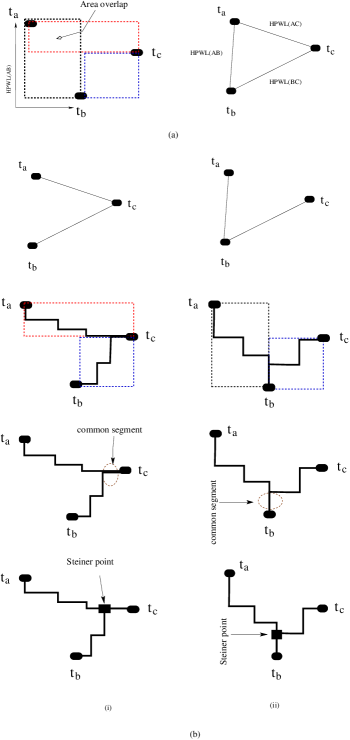
Figure 8: Multi-terminal net decomposition and Staircase Minimal Steiner Tree

We consider an example of a $3$-terminal net $n_{1}$ with terminals $\{t_{a},t_{b},t_{c}\}$ to illustrate the proposed $2$-terminal net decomposition as shown in Figure 8. In this case, $G_{c1}$, a $3$-clique, has $3$ vertices $\{t_{a},t_{b},t_{c}\}$, and $3$ edges, namely $\{t_{a},t_{b}\}$, $\{t_{b},t_{c}\}$ and $\{t_{a},t_{c}\}$, along with their corresponding edge weights (vide Figure 8 (a)). As shown in Figures 8 (b)-(i) and (b)-(ii), only one of the instances of minimum spanning tree $T_{c1}$ is greedily obtained by the said MST algorithm as the final solution.

Depending on a specific $T_{c1}$ thus obtained, the proposed $2$-terminal net segment routing, presented in the next section, for each valid terminal pair is applied. Once the routing for all the designated terminal pairs are obtained, we identify the Steiner points similar to the state-of-the-art grid-based multi-terminal net decomposition methods (FLUTE cchu ), as illustrated in Figure 8 (b). The main difference is that this work is based on a gridless framework using monotone staircase regions as the routing resources. This topology may be termed as Staircase Minimal Steiner Tree (SMST).

3.4 STAIRoute: the proposed algorithm

We present the proposed global routing algorithm STAIRoute using monotone staircase regions in Algorithm 1. This algorithm takes two inputs, namely a ordered set of nets $N$ and the junction graph $G_{j}$ as defined in Section 3.2. For each net $n_{i}\in N$, the GSRG $G_{r}^{i}$ is constructed and a routing path for the net $n_{i}$ is obtained by applying a shortest path algorithm on $G_{r}^{i}$. We have implemented $O(n^{2})$ Dijkstra’s shortest path algorithm cormen , namely DijkstraSSP(), presented in Algorithm 1.

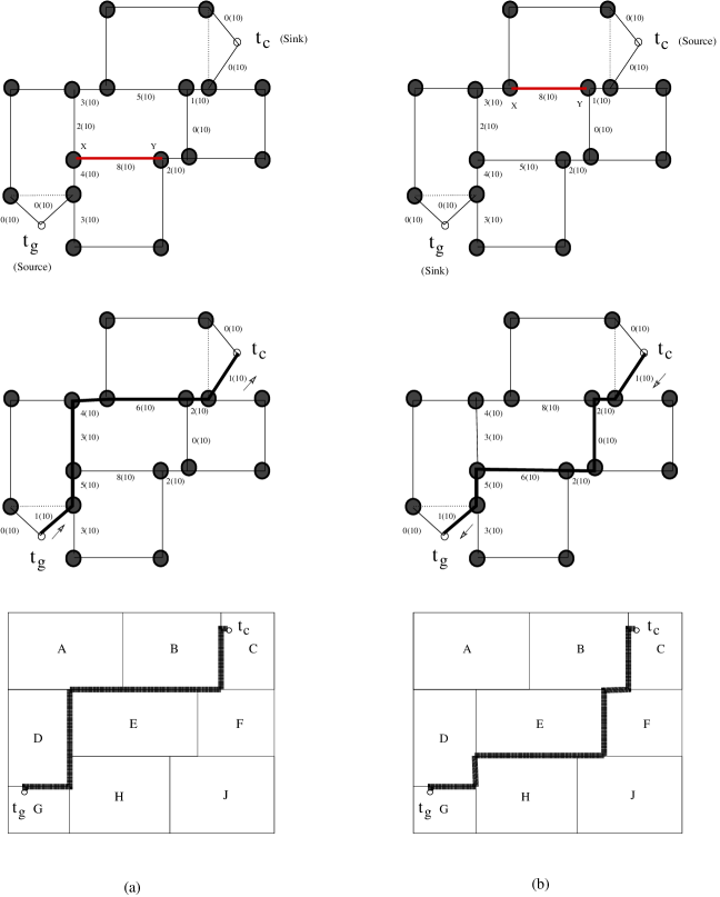
Figure 9: Exploring a routing path based on: (a) Forward Search, and (b) Backward Search

For each $2$-terminal net (segment), we consider two cases of identifying the source vertex between a pair of terminals before we apply the shortest path algorithm as:

1. the minimum $x$ coordinate (or the minimum $y$ coordinate in case both the terminals have the same $x$ coordinate)

2. the maximum $x$ coordinate (or the maximum $y$ coordinate in case both have the same $x$ coordinate)

and the procedure IdentifySource() in Algorithm 1 is used for that purpose.

We term them as Forward (FWD) and Backward (BACK) search respectively. In Figure 9 (a) and (b), we illustrate the respective cases for a $2$-terminal net {$t_{g},t_{c}$} and show that both search procedures can potentially give different routing paths. One may have a potentially better solution than the other in terms of routability, congestion scenario along with wirelength, and finally via count. The variation in wirelength due to FWD (BACK) search arises when certain resource(s) along the respective paths are fully utilized in a given metal layer; with the possibility of switching to the next available metal layer if permitted, leads to increase in the via count. Otherwise, the routing path is detoured beyond the bound box of the terminals, leading to increase in length. As long as the alternatives paths remain confined within the bounding box of the terminals, there is no variation among the respective wirelengths.

Algorithm 1 STAIRoute

0:  $G_{j}(V_{j}$,$E_{j}$), Ordered nets $N$

0:  Global routing for each $t$-terminal ($t\geq 2$) nets ($n_{i}\in N$) with 100% routability and usage $\leq$ 100%

  for all sorted nets $n_{i}\in N$ do

     $G_{r}^{i}$ = ConstructGSRG($G_{j}$,$n_{i}$)

     if Netdegree($n_{i}$) == 2 then

        /*Netdegree($n_{i}$) = Number of terminals in $n_{i}$*/

        Source = IdentifySource($n_{i}$.terminals) /*for Forward or Backward search (vide Fig. 9)*/

        Path(Source,Sink) = DijkstraSSP($G_{r}^{i}$,Source)

        if There exists a routing path from Source to Sink then

           $n_{i}$ is routed.

           Update $u_{k}$ for the respective segments.

           WireLength($n_{i}$)

           ViaCount($n_{i}$)

        else

           Routing $n_{i}$ is a failure and continue for $n_{i+1}$

        end if

     else

        $G_{c}^{i}$ = ConstructNodeClique($n_{i}$.terminals)

        $T^{i}$ = ObtainMST($G_{c}^{i}$) /*described in Section 3.3*/

        for all edges $(t_{j},t_{k})\in T^{i}$ do

           Source = IdentifySource($t_{j},t_{k}$) /*for Forward or Backward search (vide Fig. 9)*/

           Path(Source,Sink) = DijkstraSSP($G_{r}^{i}$,Source)

           if There exists a routing path from Source to Sink then

              $2$-terminal net segment is routed; calculate the segment length.

              update the $u_{k}$ for the respective segments.

           else

              Routing $n_{i}$ is a failure and continue for $n_{i+1}$

           end if

        end for

        Identify the Steiner Point(s) /*vide Fig. 8*/

        WireLength($n_{i}$)

        ViaCount($n_{i}$)

     end if

  end for

In the unreserved layer model, routing a net may incur a number of vias due to change in metal layer used to route through a set of routing resources. It does not depend on their vertical/horizontal orientation. For reserved layer model, each direction (vertical or horizontal) supports only a set of designated routing layers, e.g., horizontal layers are routed through odd numbered layers only. The number of vias along a routing path depends on the number of bends in it, i.e., the alternating (horizontal/vertical) orientation of the contiguous routing resources, for a minimum change of one metal layer among the resources along that path karb3 ; royj . Congestion in these regions may also contribute to the number of vias along a routing path, in both the cases. From the example shown in Figure 10 (a) and (b), we notice that the routing path for a given net ($t_{g}$, $t_{c}$) needs $3$ and $5$ vias for FWD and BACK searches respectively. Therefore, depending on the netlist and the floorplan topology of a given circuit, one method may dominate over the other. This method can be extended to $t$ ($>2$)-terminal nets, since we decompose those nets using the method stated earlier into $2$-terminal net segments. A better routing path for each of the resulting net segments can be obtained while employing either of the search procedures at a time.

Figure 10: Impact of search direction on via count along a routing path: (a) Forward Search with $3$ vias, and (b) Backward Search with $5$ vias

Before the routing procedure starts, it is very important that the all nets ($n_{i}\in N$) are ordered based on their half perimeter wire length (HPWL), and the number of terminals in each net, i.e., (Netdegree). The net ordering (priority) is determined based on the non-decreasing order of HPWL first and then Netdegree. A net with smaller HPWL and then Netdegree, has the precedence over other nets. The aim is to ensure that the shorter (local) nets are routed before the longer ones so as to avoid congestion in the routing resources as well as have a uniform routing distribution across the layout of the design without incurring too much detours. Here detoures imply that the routing is done along a non-monotone path such as U-shaped paths. We illustrate the working of this algorithm for $t$ ($\geq 2$)-terminal nets in Figure 6.

Theorem 1.

Given a floorplan having $n$ blocks and $k$ nets having at most $t$-terminals ($t\geq 2$), the algorithm STAIRoute takes $O(n^{2}kt)$ time.

Proof.

From Lemma 4, we say that GSRG construction takes $O(t)$ time. For each 2-terminal net routing, finding the Source vertex takes $O(n)$ and our implementation of Dijkstra’s single source shortest path algorithm (DijkstraSSP) takes $O(n^{2})$.

Again, for $t$-terminal ($t>2$) nets, computing $G_{c}^{i}$ takes $O(t^{2})$ and our implementation of Prim’s algorithm takes $O(t^{2})$. For each terminal pair ($t_{i},t_{j}$), we obtain the shortest path using DijkstraSSP in $O(n^{2})$ time. Thus, for each $t(\geq 2)$ terminal net, the time complexity is $O(t+t^{2}+n^{2}t)$, i.e., $O(n^{2}t)$, since a given net may be connected to all $n$ blocks resulting in $t=n$ in the worst case. Therefore, the overall worst case time complexity for all $k$ nets is $O(n^{2}kt)$. ∎

4 Experimental Results

We have implemented the proposed algorithm STAIRoute in C programming language and run on a 64bit Linux platform powered by Intel Core2 Duo (1.86GHz) and 2GB RAM. We used source code for top-down hierarchical monotone staircase bipartitioning algorithm implemented by karb to obtain the BAG and MSC tree data structure. We used MCNC/GSRC hard floorplanning benchmark circuits as given in Table 4. In order to test our algorithm, four different instances for each of the benchmarks were generated with a random seed using Parquet adya ; parque tool. For a given circuit, the best case (BC) and the worst case (WC) instances among a set of floorplan topologies are solely designated in the context of total half perimeter wire length (HPWL) of all the nets, as the ones with the smallest and the largest HPWL respectively.

Floorplanning Benchmarks: MCNC and GSRC Circuits Suite Circuit #Blocks #Nets Avg. Net-deg MCNC apte 9 44 3.500 hp 11 44 3.545 xerox 10 183 2.508 ami33 33 84 4.154 ami49 49 377 2.337 GSRC n10 10 54 2.129 n30 30 147 2.102 n50 50 320 2.112 n100 100 576 2.135 n200 200 1274 2.138 n300 300 1632 2.161

To the best of our knowledge, there exists no such early routability estimator at the floorplanning stage. Therefore, we believe that it is unfair to have a direct comparison of our early global routing results on a given floorplan with the existing post-placement global routing results specially by those using pattern routing such as kast ; zcao ; ychang , as they are in the different scopes of the flow. Therefore, we are restricted to compare our results with the state-of-the-art Steiner tree base routing topology estimator tool FLUTE cchu .

We present our experiments by running the proposed global routing method using HV reserved layer model restricted up to eight metals layers. We consider BC and WC floorplan topologies for each of the circuits. In these experiments, we refer to Figure 7 (a) for $3$ different capacity scaling profiles, and also refer to Figure 9 for two possible directions for exploring the possible routing paths. We iterate that all the results presented here correspond to $100\%$ routability and restricted to Under-Congestion region of Figure 5 that ensures no congestion in any routing resource. Otherwise, $100\%$ routability can not be achieved.

Following are the configurations considered for conducting the experiments on the benchmark circuits given in Table 4:

1. Forward search method with No Capacity Scaling ($FCN$)

2. Forward search method with Hyperbolic Capacity Scaling ($FCH$)

3. Forward search method with Ladder type Capacity Scaling ($FCL$)

4. Backward search method with No Capacity Scaling ($BCN$)

5. Backward search method with Hyperbolic Capacity Scaling ($BCH$)

6. Backward search method with Ladder type Capacity Scaling ($BCL$)

In Figure 11, we showcase the routing results for $n300$ for all six run configurations and two different floorplan instances, namely BC and WC. While studying these plots, we notice that the forward (backward) search with hyperbolic scaling $FCH$ ($BCH$) gives the worst results as compared to the other two configurations {$FCN,FCL$} ({$BCN,BCL$}) both in terms of routed wirelength and via count, both in case of BC and WC floorplans for a given circuit. This is due to the fact that the hyperbolic profile is the most stringent profile among the other profiles as depicted in Figure 7 (a). We also notice similar pattern for runtime as well as presented in Figure 11 (c).

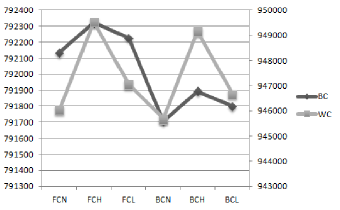
(a)

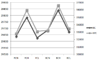
(b)

(c)

Figure 11: Plot for best case (BC) and worst case (WC) floorplan instances of $n300$ vs. different run configurations: (a) Wirelength ($\mu$m), (b) Via Count, and (c) Runtime(sec)

Next, we focus on the corresponding results obtained for the remaining configurations {$FCN,FCL$} ({$BCN,BCL$}) for both BC and WC floorplan topologies. Figure 11 (a) shows that $FCN$ ($BCN$) gives better wirelength against $FCL$ ($BCL$) both in BC and WC. Although it reflects a similar trend in the respective via count for the WC topology, $FCL$ ($BCL$) has better via count as compared to $FCN$ ($BCN$) in BC (Figure 11 (b)). We conduct another set of comparison for wirelength and via count between $FCN$ and $BCN$ ($FCL$ and $BCL$) for both BC and WC. Although backward search produces better wirelength as compared to that in forward search method, it incurs more vias to route a set of nets than its counterpart. This clearly shows that an early routing solution not only depends on the search direction and the capacity profiles, but also on different floorplan instances of the same circuit.

Wirelength for different run configurations against FLUTE cchu length: for BC floorplan instances only Circuit $FCN$($\mu$m) $FCH$($\mu$m) $FCL$($\mu$m) $BCN$($\mu$m) $BCH$($\mu$m) $BCL$($\mu$m) FLUTE($F$) ($FCN/F$) ($FCH/F$) ($FCL/F$) ($BCN/F$) ($BCH/F$) ($BCL/F$) ($\mu$m) apte 398137.031 398411.250 398137.031 396034.313 396308.563 396034.313 338628.000 (1.1757) (1.1765) (1.1757) (1.1695) (1.1703) (1.1695) hp 201996.672 203060.359 201996.672 211536.609 210086.344 211536.609 123716.000 (1.6327) (1.6413) (1.6327) (1.7099) (1.6981) (1.7099) xerox 716916.688 717291.625 716916.688 710575.375 710575.375 710575.375 633533.000 (1.1316) (1.1322) (1.1316) (1.1216) (1.1216) (1.1216) ami33 111126.102 111563.070 111126.102 111481.008 111896.906 111481.008 92330.000 (1.2036) (1.2083) (1.2036) (1.2074) (1.2119) (1.2074) ami49 1925760.875 2009223.625 1925760.875 1926176.750 2010630.125 1926176.750 1608746.000 (1.1971) (1.2489) (1.1971) (1.1973) (1.2498) (1.1973) n10 19837.000 19837.000 19837.000 18497.500 18497.500 18497.500 16626.000 (1.1931) (1.1931) (1.1931) (1.1126) (1.1126) (1.1126) n30 59585.000 59585.000 59585.000 58761.500 58761.500 58761.500 49370.000 (1.2069) (1.2069) (1.2069) (1.1902) (1.1902) (1.1902) n50 151604.000 152119.000 151851.000 150741.000 151256.000 150988.000 125018.000 (1.2127) (1.2168) (1.2146) (1.2058) (1.2099) (1.2077) n100 251455.500 252647.500 251476.500 250771.000 251917.000 250792.000 212112.000 (1.1855) (1.1911) (1.1856) (1.1823) (1.1877) (1.1824) n200 429854.500 430043.500 429923.500 428987.000 429128.000 429056.000 381021.000 (1.1282) (1.1287) (1.1283) (1.1259) (1.1263) (1.1261) n300 792135.000 792323.000 792229.000 791707.500 791895.500 791801.500 699006.000 (1.1332) (1.1335) (1.1334) (1.1326) (1.1329) (1.1328)

In Table 4 (4), we summarize the wirelength obtained for all the circuits in all the configurations for the respective BC (WC) topologies and compare them with the corresponding FLUTE cchu length. For a given configuration, the corresponding wirelength is accompanied by its ratio of wirelength and FLUTE length, e.g., $FCN/F$ in the bracket below it and the best ratio(s) are highlighted. It is evident that from these results that, except for the circuits with $100$ or more blocks, the length ratio pairs $FCN/F$ and $FCL/F$ ($BCN/F$ and $BCL/F$) have little variation and also shows that $BCN$ yields the best wirelength of a given circuit with respect to the corresponding FLUTE length for most of the circuits. The best results among all the run configurations are highlighted in bold letters.

Wirelength for different run configurations against FLUTE cchu length: for WC floorplan instances only Circuit $FCN$($\mu$m) $FCH$($\mu$m) $FCL$($\mu$m) $BCN$($\mu$m) $BCH$($\mu$m) $BCL$($\mu$m) FLUTE($F$) ($FCN/F$) ($FCH/F$) ($FCL/F$) ($BCN/F$) ($BCH/F$) ($BCL/F$) ($\mu$m) apte 450376.469 450376.469 450376.469 438912.781 439198.781 438912.781 389806.000 (1.1554) (1.1554) (1.1554) (1.1260) (1.1267) (1.1260) hp 232782.313 232782.313 232782.313 230255.938 230255.938 230255.938 144993.000 (1.6055) (1.6055) (1.6055) (1.5880) (1.5880) (1.5880) xerox 1542729.875 1590995.125 1542729.875 1511243.250 1558185.250 1511243.250 1391401.000 (1.1088) (1.1434) (1.1088) (1.0861) (1.1199) (1.0861) ami33 120903.578 120903.578 120903.578 118746.414 118969.086 118746.414 105025.000 (1.1512) (1.1512) (1.1512) (1.1306) (1.1328) (1.1306) ami49 1914369.375 1914369.375 1914369.375 1898528.125 1898528.125 1898528.125 1684114.000 (1.1367) (1.1367) (1.1367) (1.1273) (1.1273) (1.1273) n10 24526.500 25116.500 24526.500 23707.500 24297.500 23707.500 20012.000 (1.2256) (1.2551) (1.2256) (1.1847) (1.2141) (1.1847) n30 74743.500 75105.500 74838.500 74151.500 74513.500 74246.500 59879.000 (1.2482) (1.2543) (1.2498) (1.2384) (1.2444) (1.2399) n50 187971.000 189752.000 188476.000 187197.000 188994.000 187702.000 158173.000 (1.1884) (1.1996) (1.1916) (1.1835) (1.1949) (1.1867) n100 277304.500 277950.500 277583.500 276545.000 277251.000 276824.000 238841.000 (1.1610) (1.1637) (1.1622) (1.1579) (1.1608) (1.1590) n200 836136.000 865590.000 837493.000 835535.500 864329.500 836928.500 749479.000 (1.1156) (1.1549) (1.1174) (1.1148) (1.1532) (1.1167) n300 946039.500 949547.500 947076.500 945688.500 949165.500 946675.500 830035.000 (1.1398) (1.1440) (1.1410) (1.1393) (1.1435) (1.1405)

In Table 4, we present the via count for all the run configurations for each circuit for BC (WC in brackets) instances. The results clearly point out the consequence of forward and backward search on via count. It is also evident that via count in case of $FCH$ ($BCH$) is the worst among all other two configurations, namely {$FCN,FCL$} ({$BCN,BCL$}), as we have seen in case of wirelength. There is little variation in via count for relatively smaller circuits in case of {$FCN,FCL$} ({$BCN,BCL$}) and becomes significant for relatively larger circuits. The best via count (highlighted with bold letters) for each circuit in both BC and WC (in brackets) is mostly obtained in case of {$FCN,FCL$}.

Via count for different run configurations: for BC (WC in brackets)
floorplan instance Circuit $FCN$ $FCH$ $FCL$ $BCN$ $BCH$ $BCL$ apte 404 508 404 412 504 412 (452) (660) (452) (460) (656) (460) hp 502 720 502 536 730 536 (430) (630) (430) (430) (626) (430) xerox 1190 1238 1190 1220 1272 1220 (1401) (2261) (1401) (1527) (2369) (1547) ami33 1156 1500 1156 1162 1530 1162 (1240) (1528) (1240) (1234) (1586) (1234) ami49 3290 4466 3290 3406 4676 3406 (3629) (3789) (3629) (3877) (4137) (3877) n10 176 176 176 176 176 176 (220) (278) (220) (222) (260) (222) n30 937 941 937 956 960 956 (1047) (1100) (1014) (1059) (1108) (1026) n50 3194 3609 3184 3191 3598 3181 (3252) (5089) (3296) (3402) (5078) (3442) n100 6748 7553 6748 6795 7623 6799 (7742) (10050) (7746) (7846) (10146) (7850) n200 18016 18040 18008 17977 17993 17969 (16905) (26828) (17610) (17253) (27041) (17571) n300 29639 29785 29627 29687 29841 29675 (32814) (35955) (33093) (33235) (36624) (33461)

In our congestion analysis, we focus on relative congestion (ration of routing demand $u$ and capacity $r$) instead of absolute congestion measured by total overflow in any routing resource (edge in case of grid graph model). This leads us to follow the method prescribed in wei in order to analyze the global congestion scenario in a given floorplan instance. The authors in wei used relative congestion (ratio of routing demand and routing capacity) in any edge of grid graph model instead of absolute congestion, i.e., estimating total overflow by computing excess routing demand with respect to the capacity over all edges. They proposed a new metric called average congestion per edge based on relative congestion for a certain percentage of top congested edges among all congested edges. This is denoted as $ACE(x\%)$ where $x$ is the percentage value of the worst congested edges. Based on this metric, an weighted average of $ACE(x\%)$ for four different values of $x={0.5,1,2,5}$ is computed and denoted as $wACE4$. In this work, we adopt a similar way to compute related congestion as normalized usage (vide Equation 2).

In Table 4, we capture the $wACE4$ values among all layers for each circuit for all the run configurations in BC and WC (in brackets) to showcase the corresponding congestion scenario when $100\%$ routability is achieved. The results validate that our method conforms to the congestion profile depicted in Figure 5 and does not cross the value of $1.0$ in any case. The results presented in this table correspond to the maximum $wACE4$ value for a given circuit and the one with best value among all the configurations is highlighted with bold.

Congestion (wACE4) for different run configurations: for BC (WC in brackets)
floorplan instance Circuit $FCN$ $FCH$ $FCL$ $BCN$ $BCH$ $BCL$ apte 0.9011 0.8384 0.9011 0.9449 0.9063 0.9449 (0.8738) (0.9861) (0.8738) (0.7971) (0.8750) (0.7971) hp 0.9914 0.9871 0.9914 0.9871 0.9853 0.9871 (0.9906) (0.8135) (0.9906) (0.9906) (0.8021) (0.9906) xerox 0.6229 0.6139 0.6229 0.6229 0.6090 0.6229 (0.9940) (0.9375) (0.9940) (0.9583) (0.9375) (0.9583) ami33 0.9673 0.6874 0.9673 0.9712 0.6920 0.9712 (0.9388) (0.9944) (0.9388) (0.9120) (0.8102) (0.9120) ami49 0.9750 0.9931 0.9750 0.9750 0.9976 0.9750 (0.7129) (0.7215) (0.7129) (0.7115) (0.7068) (0.7115) n10 0.6435 0.6435 0.6435 0.6435 0.7670 0.6435 (0.9625) (0.9500) (0.9625) (0.9625) (0.9500) (0.9625) n30 0.6585 0.9826 0.6585 0.6570 0.9788 0.6570 (0.9547) (0.9667) (0.9547) (0.9546) (0.9500) (0.9546) n50 0.8179 0.6627 0.8209 0.8163 0.6343 0.8182 (0.8399) (0.8246) (0.8488) (0.8644) (0.8351) (0.8733) n100 0.9904 0.9772 0.9904 0.9871 0.9883 0.9871 (0.9187) (0.9974) (0.9187) (0.9282) (0.9984) (0.9282) n200 0.4892 0.8269 0.4892 0.4831 0.8152 0.4831 (0.8750) (0.6793) (0.8555) (0.8923) (0.6463) (0.8328) n300 0.6561 0.9863 0.6561 0.6681 0.9843 0.6681 (0.9813) (0.9964) (0.9811) (0.9774) (0.9903) (0.9770)

In Table 4, we report runtime in seconds for all the circuits versus the said run configurations. These results correspond to both BC and WC (in brackets) floorplan instances. As we can see that the best (as highlighted) runtime in the context of BC and WC (in brackets) floorplan instances for a given circuit is given by either $FCL$ or $BCL$ for most of the cases.

Runtime (sec) for different run configurations: for BC (WC in brackets)
floorplan instance Circuit $FCN$ $FCH$ $FCL$ $BCN$ $BCH$ $BCL$ apte 0.114 0.109 0.103 0.108 0.109 0.113 (0.112) (0.106) (0.102) (0.103) (0.104) (0.103) hp 0.115 0.107 0.105 0.107 0.102 0.103 (0.114) (0.107) (0.100) (0.107) (0.102) (0.101) xerox 0.126 0.124 0.122 0.122 0.121 0.121 (0.140) (0.125) (0.116) (0.130) (0.125) (0.120) ami33 0.172 0.167 0.151 0.161 0.159 0.156 (0.186) (0.178) (0.158) (0.158) (0.166) (0.170) ami49 0.464 0.453 0.438 0.441 0.458 0.442 (0.483) (0.465) (0.446) (0.463) (0.465) (0.460) n10 0.122 0.099 0.101 0.101 0.101 0.102 (0.109) (0.101) (0.105) (0.103) (0.105) (0.102) n30 0.181 0.164 0.166 0.164 0.160 0.164 (0.162) (0.161) (0.153) (0.163) (0.164) (0.157) n50 0.423 0.410 0.398 0.414 0.399 0.396 (0.449) (0.437) (0.440) (0.444) (0.441) (0.432) n100 2.480 2.408 2.412 2.399 2.445 2.386 (2.076) (2.096) (2.064) (2.073) (2.070) (2.054) n200 18.342 18.741 17.718 18.201 18.175 17.533 (21.472) (20.885) (20.909) (21.452) (21.315) (20.625) n300 53.151 54.596 50.929 52.739 53.656 51.730 (57.993) (58.719) (55.090) (55.856) (58.742) (57.069)

4.1 Results for IBM HB benchmarks

In this paper, we also used IBM HB floorplanning benchmarks hben in Table 4.1 for verifying the proposed early global routing method STAIRoute. These benchmarks were derived from ISPD98 placement benchmark circuits with certain modifications (see hben for details). These floorplan instances for each circuit were generated using Parquet adya ; parque using random seed.

IBM HB Floorplanning Benchmark Circuits hben Circuit #Blocks #Nets Avg. HPWL Name NetDeg ($10^{6}\mu$m) ibm01 2254 3990 3.94 8.98 ibm02 3723 7393 4.84 22.19 ibm03 3227 7673 4.18 23.83 ibm04 4050 9768 3.92 30.82 ibm05 1612 7035 5.58 18.12 ibm06 1902 7045 4.92 21.78 ibm07 2848 10822 4.44 42.48 ibm08 3251 11250 4.92 46.57 ibm09 2847 10723 4.08 48.35 ibm10 3663 15590 3.85 121.23

As mentioned earlier, we can not directly compare our results with that of the state-of-the-art post-placment global routers. As a results, we come up with an indirect approach to compare wirelength obtained for each circuit, by normalizing it with steiner length computed by FLUTE cchu . The comparison results are summarized in Table 4.1 and shown that the values related STAIRoute only marginally higher. This is due to the fact that STAIRoute does not have the scope of routing the tiny nets that connect the standard cells, while the others presented in the table perform those tiny nets as well, in addition to the longer nets that can also be abstracted at the flooplanning level.

Normalized (w.r.t Steiner length cchu ) wirelength between the existing
post-placement global routers and STAIRoute Circuit Post-placement Global Routers STAIRoute^c Name ozdal ^b mcho1 ^b zhang2 ^b royj ^b moffit ^b ychang ^b ibm01 1.071 1.042 1.068 1.053 1.059 1.039 1.156 ibm02 1.036 1.032 1.038 1.018 1.027 1.024 1.175 ibm03 1.007 1.007 1.007 1.005 1.010 1.005 1.175 ibm04 1.045 1.028 1.046 1.027 1.045 1.023 1.155 ibm05^d - - - - - - 1.198 ibm06 1.011 1.007 1.013 1.006 1.013 1.007 1.166 ibm07 1.018 1.006 1.015 1.007 1.016 1.007 1.192 ibm08 1.005 1.008 1.009 1.006 1.010 1.006 1.197 ibm09 1.007 1.006 1.009 1.004 1.011 1.008 1.199 ibm10 1.016 1.027 1.015 1.008 1.020 1.010 1.187 Average 1.024 1.018 1.024 1.015 1.024 1.014 1.180 $b$ - using ISPD98 global routing benchmarks, $c$ - using IBM-HB floorplanning benchmarks, and $d$ - no result on $ibm05$ of ISPD98 benchmark by the existing global routers

5 Conclusion

In this paper, we proposed a novel early global routing framework based on monotone staircase regions obtained by hierarchical bipartitioning of a given flooplan instances of a circuit. It thus immediately follows the floorplanning stage in the existing VLSI implementation flow and hence require no detailed placement of standard cells in order to conduct global routing of the nets available at this level of design abstraction. Unlike the existing global routers following the standard cell placement stage, the monotone staircase regions act as the routing resources and the nets are routed though them for a given number of metal layers. Both unreserved or reserved layer model can be used in this framework. The congestion scenario is modeled in this routing model in such way that the utilization is no more than $100\%$ in any of the routing resources, by switching to next permissible layer. Multi-terminal net decomposition using the proposed Steiner tree method is unique and no other existing methods are known to have a similar model. Our experimental results show that $100\%$ routing completion is possible without any congestion even for different capacity profiles that include constrained metal pitch/width variation due to recent fabrication processes. Additionally, employing different search directions shows that improvement in routed wirelength and via count may potentially be achieved.

The proposed framework has a two fold potential advantage: (a) evaluate the given floorplan on the basis of early global routing results obtained by STAIRoute, and (b) estimate the global routing metrics and related information essential for the subsequent stages of the design flow. This work may be extended to incorporate design for manufacturability (DFM) issues by suitably modeling them into the routing cost.

References

- [1] Roy, J.A., Markov, I.L.: ‘High-Performance Routing at the Nanometer Scale’, Computer-Aided Design of Integrated Circuits and Systems, IEEE Transactions on, 2008, 27, (6), pp. 1066–1077
- [2] Pan, M., Chu, C. ‘FastRoute: A Step to Integrate Global Routing into Placement’. In: Computer-Aided Design, 2006. ICCAD ’06. IEEE/ACM International Conference on. (, 2006. pp. 464–471
- [3] Lee, T.H., Wang, T.C.: ‘Congestion-Constrained Layer Assignment for Via Minimization in Global Routing’, Computer-Aided Design of Integrated Circuits and Systems, IEEE Transactions on, 2008, 27, (9), pp. 1643–1656
- [4] Sherwani, N.A.: ‘Algorithms for VLSI Physical Design Automation’. 2nd ed. (Norwell, MA, USA: Kluwer Academic Publishers, 1995)
- [5] Sur.Kolay, S., Bhattacharya, B.B. ‘The cycle structure of channel graphs in nonsliceable floorplans and a unified algorithm for feasible routing order’. In: IEEE International Conference on Computer Design: VLSI in Computers and Processors. (, 1991. pp. 524–527
- [6] Guruswamy, M., Wong, D.F. ‘Channel routing order for building-block layout with rectilinear modules’. In: IEEE International Conference on Computer-Aided Design (ICCAD-89) Digest of Technical Papers. (, 1988. pp. 184–187
- [7] Kastner, R., Bozorgzadeh, E., Sarrafzadeh, M.: ‘Pattern routing: use and theory for increasing predictability and avoiding coupling’, Computer-Aided Design of Integrated Circuits and Systems, IEEE Transactions on, 2002, 21, (7), pp. 777–790
- [8] Cao, Z., Jing, T.T., Xiong, J., Hu, Y., Feng, Z., He, L., et al.: ‘Fashion: A Fast and Accurate Solution to Global Routing Problem’, Computer-Aided Design of Integrated Circuits and Systems, IEEE Transactions on, 2008, 27, (4), pp. 726–737
- [9] Chang, Y.J., Lee, Y.T., Gao, J.R., Wu, P.C., Wang, T.C.: ‘NTHU-Route 2.0: A Robust Global Router for Modern Designs’, IEEE Transactions on Computer-Aided Design of Integrated Circuits and Systems, 2010, 29, (12), pp. 1931–1944
- [10] Lu, J., Sham, C.W. ‘LMgr: A low-Memory global router with dynamic topology update and bending-aware optimum path search’. In: Quality Electronic Design (ISQED), 2013 14th International Symposium on. (, 2013. pp. 231–238
- [11] Kar, B., Sur.Kolay, S., Mandal, C. ‘Global Routing Using Monotone Staircases with Minimal Bends’. In: 2014 27th International Conference on VLSI Design, VLSID 2014, Mumbai, India, January 5-9, 2014. (, 2014. pp. 369–374
- [12] Cho, M., Lu, K., Yuan, K., Pan, D.Z.: ‘BoxRouter 2.0: A Hybrid and Robust Global Router with Layer Assignment for Routability’, ACM Trans Des Autom Electron Syst, 2009, 14, (2), pp. 32:1–32:21. Available from: http://doi.acm.org/10.1145/1497561.1497575
- [13] Dai, K.R., Liu, W.H., Li, Y.L.: ‘NCTU-GR: Efficient Simulated Evolution-Based Rerouting and Congestion-Relaxed Layer Assignment on 3-D Global Routing’, Very Large Scale Integration (VLSI) Systems, IEEE Transactions on, 2012, 20, (3), pp. 459–472
- [14] Liu, W.H., Kao, W.C., Li, Y.L., Chao, K.Y.: ‘NCTU-GR 2.0: Multithreaded Collision-Aware Global Routing With Bounded-Length Maze Routing’, Computer-Aided Design of Integrated Circuits and Systems, IEEE Transactions on, 2013, 32, (5), pp. 709–722
- [15] Kar, B., Sur.Kolay, S., Rangarajan, S.H., Mandal, C. ‘A faster hierarchical balanced bipartitioner for VLSI floorplans using Monotone Staircase Cuts’. In: Progress in VLSI Design and Test - 16th International Symposium, VDAT 2012, Shibpur, India, July 1-4, 2012. Proceedings. (, 2012. pp. 327–336
- [16] Dasgupta, P., Pan, P., Nandy, S.C., Bhattacharya, B.B.: ‘Monotone Bipartitioning Problem in a Planar Point Set with Applications to VLSI’, ACM Trans Des Autom Electron Syst, 2002, 7, (2), pp. 231–248. Available from: http://doi.acm.org/10.1145/544536.544537
- [17] Majumder, S., Sur.Kolay, S., Nandy, S.C., Bhattacharya, B.B.: ‘On Finding a Staircase Channel with Minimum Crossing Nets in a VLSI Floorplan’, Journal of Circuits, Systems and Computers, 2004, 13, (05), pp. 1019–1038. Available from: http://www.worldscientific.com/doi/abs/10.1142/S0218126604001854
- [18] Majumder, S., Sur.Kolay, S., Bhattacharya, B.B., Das, S.K.: ‘Hierarchical partitioning of VLSI floorplans by staircases’, ACM Trans Design Autom Electr Syst, 2007, 12, (1). Available from: http://doi.acm.org/10.1145/1217088.1217095
- [19] Yang, H., Wong, D.F. ‘Efficient Network Flow Based Min-cut Balanced Partitioning’. In: IEEE/ACM International Conference on Computer-Aided Design. (, 1994. pp. 50–55
- [20] ‘EE Times: Layer-aware Optimization’. (, . Available from: https://www.eetimes.com/document.asp?doc_id=1279842
- [21] Chu, C., Wong, Y.C.: ‘FLUTE: Fast Lookup Table Based Rectilinear Steiner Minimal Tree Algorithm for VLSI Design’, Computer-Aided Design of Integrated Circuits and Systems, IEEE Transactions on, 2008, 27, (1), pp. 70–83
- [22] Hanan, M.: ‘On Steiner’s Problem with Rectilinear Distance’, SIAM Journal on Applied Mathematics, 1966, 14, (2), pp. 255–265. Available from: http://dx.doi.org/10.1137/0114025
- [23] Cormen, T.H., Leiserson, C.E., Rivest, R.L., Stein, C.: ‘Introduction to Algorithms’. 3rd ed. (Cambridge, MA, USA: MIT Press, 2009)
- [24] Adya, S.N., Markov, I.L.: ‘Fixed-outline floorplanning: Enabling hierarchical design’, IEEE Transactions on Very Large Scale Integration (VLSI) Systems, 2003, 11, (6), pp. 1120–1135
- [25] ‘Parquet floorplanner and mcnc/gsrc floorplanning benchmarks’. (, . Available from: https://vlsicad.eecs.umich.edu/BK/parquet
- [26] Wei, Y., Sze, C., Viswanathan, N., Li, Z., Alpert, C.J., Reddy, L., et al. ‘GLARE: Global and local wiring aware routability evaluation’. In: Design Automation Conference (DAC), 2012 49th ACM/EDAC/IEEE. (, 2012. pp. 768–773
- [27] ‘IBM-HB Floorplanning Benchmarks’. (, . Available from: https://cadlab.cs.ucla.edu/cpmo/HBsuite.html
- [28] Ozdal, M.M., Wong, M.D.F.: ‘Archer: A History-Based Global Routing Algorithm’, IEEE Transactions on Computer-Aided Design of Integrated Circuits and Systems, 2009, 28, (4), pp. 528–540
- [29] Zhang, Y., Xu, Y., Chu, C. ‘FastRoute3.0: A fast and high quality global router based on virtual capacity’. In: Computer-Aided Design, 2008. ICCAD 2008. IEEE/ACM International Conference on. (, 2008. pp. 344–349
- [30] Moffitt, M.D.: ‘MaizeRouter: Engineering an Effective Global Router’, IEEE Transactions on Computer-Aided Design of Integrated Circuits and Systems, 2008, 27, (11), pp. 2017–2026